Counterflows in viscous electron-hole fluid

Abstract

In ultra-pure conductors, collective motion of charge carriers at relatively high temperatures may become hydrodynamic such that electronic transport may be described similarly to a viscous flow. In confined geometries (e.g., in ultra-high quality nanostructures), the resulting flow is Poiseuille-like. When subjected to a strong external magnetic field, the electric current in semimetals is pushed out of the bulk of the sample towards the edges. Moreover, we show that the interplay between viscosity and fast recombination leads to the appearance of counterflows. The edge currents possess a non-trivial spatial profile and consist of two stripe-like regions: the outer stripe carrying most of the current in the direction of the external electric field and the inner stripe with the counterflow.

Recently, signatures of the hydrodynamic behavior of charge carriers have been observed in graphene exg1 ; exg2 ; exg3 , palladium cobaltate exp , and the Weyl semimetal WP₂ exw . This phenomenon occurs in the intermediate temperature regime, where the typical length scale of electron-electron interaction, $\ell_{ee}$, is much shorter than any other relevant scale in the problem including those characterizing scattering off potential disorder and electron-phonon scattering, ${\ell_{ee}\ll\ell_{\rm dis},\ell_{ph}}$. In this case, the independent particle approximation is violated, the motion of charge carriers becomes collective, and transport properties of the system are determined by interaction us1 ; luk .

Viscous electronic fluids exhibit unusual transport properties us1 ; luk , such as superballistic transport exg3 ; mor ; lev , nonlocal resistivity exg1 ; fal , and negative magnetoresistance exw ; gul ; pal ; moore ; als . The latter effect may also occur in two-component systems (e.g., semimetals or narrow-band semiconductors) near the charge neutrality point usp . In such systems, response of the charge carriers to the external magnetic field is non-universal depending on the interplay between inelastic scattering processes and sample geometry.

In the hydrodynamic regime, electronic transport can be described with the help of the linearized hydrodynamic theory pal ; moore ; als ; usp generalizing the standard Navier-Stokes equation dau6 . The parameters of the theory, including the shear viscosity coefficient, $\eta_{xx}$, and quasiparticle recombination time, $\tau_{R}$, can be derived, at least in principle, from the kinetic equation approach (for a particular case of graphene, see Ref. hyd, ). Due to the above two processes, the electric current density in a finite-sized sample is nonuniform. In long samples (where the length is much larger than the width, ${L\gg{W}}$), viscous effects tend to form a Poiseuille-like flow. The actual profile of the current density depends on the ratio of the typical length scale describing the viscous effects, the so-called Gurzhi length usp , $\ell_{G}(B)$, and the sample width, $W$. In the limit where the Gurzhi length exceeds the width, ${\ell_{G}\gg{W}}$, the current density profile is parabolic, similarly to the standard viscous flow dau6 ; poi . In the opposite case, the current density profile resembles the catenary curve usp , where significant inhomogeneities are localized at the sample edges. In both cases, the electric charge is being transmitted mostly through the bulk, avoiding the edges (this effect is the physical origin of the superballistic transport found in Refs. exg3, ; lev, ).

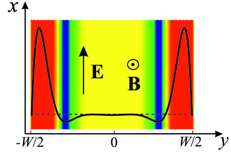
Figure 1: Schematic plot of the inhomogeneous electric current density in the regime of fast recombination and strong enough magnetic field. The color map emphasises the positive (i.e., parallel to the external electric field) current at the edge (red) contrasted to the negative (i.e., opposite to the external electric field) current in the intermediate stripe (blue). The black curve illustrates the magnitude of the current density at a given point along the sample. The dashed line indicates the zero value of the current.

Two-component systems may possess an additional inelastic scattering process: the electron-hole recombination. This process is known to create a boundary layer us2 ; us3 ; meg characterized by linear magnetotransport gus ; mol ; vas . In general, the recombination boundary layer coexists with the above viscous boundary layer. In the hydrodynamic regime, the typical time scale describing the recombination processes is much longer than the electron-electron relaxation time, ${\tau_{R}\gg\tau_{ee}}$. Since the latter defines the Gurzhi length in the absence of the magnetic field, this can be recast in the relation of the corresponding length scales, ${\ell_{R}\gg\ell_{G}(0)}$. Both length scales decrease with the applied magnetic field. The decrease of the Gurzhi length follows from the field dependence of the shear viscosity pal ; moore and is governed by the electron-electron scattering. In contrast, the effective length scale associated with the recombination processes follows from the solution of the hydrodynamic equations usp ; us2 ; us3 and is governed by the dominant elastic scattering process. In the previous paper usp , we have considered the limit of weak (or slow) recombination, where $\tau_{R}$ is much longer than the elastic mean free path and hence the recombination length is much longer than the Gurzhi length for an arbitrary magnetic field, ${\ell_{R}\gg\ell_{G}}$. In this limit, the system exhibits unconventional transport properties. For typical parameter values, the magnetoresistance of a long sample is a nonmonotonic function of the field: it is negative in weak fields and then becomes positive and linear in strong fields.

In this paper, we consider the opposite limit of relatively fast recombination, such that the recombination time, $\tau_{R}$, is much smaller than the elastic mean free path. We show that in this case the electric current density is strongly inhomogeneous and, in contrast to the standard Poiseuille flow, is mostly concentrated at the sample edges. The structure of the edge currents is most peculiar and consists of two regions, see Fig. 1. While the wider, outer region carries the large current in the direction of the applied electric field, the current in the narrower inner region flows in the opposite direction. The latter counterpropagating current is much smaller than the former, such that the total current is parallel to the electric field. However, this system exhibits a most curious example where a local current density is directed opposite to the external electric field.

Although we are focusing on a specific model of a compensated semimetal, the phenomenon of the counterflow is more general. Similar effects have been suggested in the context of the ac transport moe ; aac . Counterflows in a steady state, thermoelectric flow in a single-component electron fluid (e.g. in doped graphene or a semiconductor) will be discussed in a subsequent publication usf .

I Hydrodynamics of compensated semimetals

The hydrodynamic model of a two-component conductor with electron-hole recombination was discussed in Ref. usp, . Here we repeat the main points for completeness.

Recombination processes violate the particle number conservation for each individual constituent of the system. As a result, the continuity equations have the form

$$\frac{\partial\delta n_{\alpha}}{\partial t}+\boldsymbol{\nabla}\cdot\boldsymbol{j}_{\alpha}=-\frac{\delta n_{e}+\delta n_{h}}{2\tau_{R}},$$ (1)

where $\alpha=e,h$ distinguishes the type of carriers, $\delta n_{\alpha}$ are the deviations of the carrier densities from their equilibrium values $n_{\alpha}^{(0)}$, $\boldsymbol{j}_{\alpha}$ are the carrier currents, and $\tau_{R}$ is the electron-hole recombination time.

In the hydrodynamic regime, charge transport can be described by the generalized Navier-Stokes equation. Within linear response, the equations for the two constituent of the system have the form usp

$$\frac{\partial\boldsymbol{j}_{\alpha}}{\partial t}+\frac{\langle v^{2}\rangle}{2}\boldsymbol{\nabla}\delta n_{\alpha}-\frac{e_{\alpha}n_{\alpha}^{(0)}}{m}\boldsymbol{E}-\omega_{\alpha}\left[\boldsymbol{j}_{\alpha}\times\boldsymbol{e}_{z}\right]=$$ (2)

$$\qquad\qquad\qquad\qquad\qquad=-\frac{\boldsymbol{j}_{\alpha}}{\tau}-\frac{\boldsymbol{j}_{\alpha}-\boldsymbol{j}_{\alpha^{\prime}}}{2\tau_{eh}}+\eta_{xx}\Delta\boldsymbol{j}_{\alpha}.$$

Here we consider the orthogonal magnetic field, ${\boldsymbol{B}\!=\!B\boldsymbol{e}_{z}}$; the electron and hole charges are ${e_{h}\!=\!e>0}$, ${e_{e}\!=\!-e}$, and the cyclotron frequencies are ${\omega_{\alpha}\!=\!e_{\alpha}{B}/(mc)\!=\!\omega_{c}e_{\alpha}/e}$; the index $\alpha^{\prime}$ denotes the constituent other than $\alpha$: ${\alpha^{\prime}\!=\!e}$ for ${\alpha\!=\!h}$ and vice versa; $\tau_{eh}$ is the momentum relaxation time due to electron-hole scattering; and the averaging (for the parabolic spectrum with the constant density of states $\nu_{0}$) is defined as usg

$$\langle\dots\rangle\!=\!-\!\!\int\!\!d\epsilon\,\frac{\partial f^{(0)}(\epsilon)}{\partial\epsilon}(\dots),$$

where $f^{(0)}(\epsilon)$ is the Fermi distribution function. The choice of the parabolic bands simplifies the algebra, but is not essential; all qualitative features of our results remain valid for an arbitrary spectrum (respecting the rotational invariance jul ).

The field-dependent shear viscosity is given by pal ; st

$$\eta_{xx}\!=\!\eta_{0}/(1\!+\!4\omega_{c}^{2}\tau_{ee}^{2}),$$ (3)

where $\eta_{0}$ is the shear viscosity in the absence of the magnetic field

$$\eta_{0}\!=\!\langle v^{4}\rangle\tau_{ee}/(4\langle v^{2}\rangle)\sim\langle v^{2}\rangle\tau_{ee}.$$ (4)

The off-diagonal (or Hall) viscosity is neglected in Eq. (2) since the corresponding contribution is much smaller than the Lorentz terms, see Ref. usp, for details.

The hydrodynamic theory is justified if the electron-electron scattering time $\tau_{ee}$ is the shortest time scale in the problem (including the “ballistic” time defined by the sample width)

$$\tau_{ee}\ll\tau,\tau_{R},\tau_{eh},\tau_{W},\qquad\tau_{W}\sim W/\sqrt{\langle v^{2}\rangle}.$$ (5)

In this case, the equations (2) describe the two (electron and hole) fluids that are weakly coupled by electron-hole scattering mor ; us2 ; us3 ; svi . Unlike the single-component fluid considered in Ref. pal, , these two fluids cannot be considered as incompressible. However, under the assumption (5) electron-hole recombination dominates the viscous compressibility (related to bulk viscosity) allowing us to drop the latter from Eqs. (2).

In this paper we restrict our consideration to charge neutrality, ${n_{e}=n_{h}}$. Introducing the total quasiparticle density, ${\rho\!=\!n_{e}\!+\!n_{h}}$ and the linear combinations of the two currents, ${\boldsymbol{P}\!=\!\boldsymbol{j}_{e}\!+\!\boldsymbol{j}_{h}}$ and ${\boldsymbol{j}\!=\!\boldsymbol{j}_{h}\!-\!\boldsymbol{j}_{e}}$, we re-write the hydrodynamic theory (1) and (2) as

$$\frac{\partial\delta\rho}{\partial t}+\boldsymbol{\nabla}\cdot\boldsymbol{P}=-\frac{\delta\rho}{\tau_{R}},\qquad\boldsymbol{\nabla}\cdot\boldsymbol{j}=0,$$ (6a)

$$\frac{\partial\boldsymbol{P}}{\partial t}+\frac{\langle v^{2}\rangle}{2}\boldsymbol{\nabla}\delta\rho-\omega_{c}\left[\boldsymbol{j}\times\boldsymbol{e}_{z}\right]=-\frac{\boldsymbol{P}}{\tau}+\eta_{xx}\Delta\boldsymbol{P},$$ (6b)

$$\frac{\partial\boldsymbol{j}}{\partial t}-\frac{e\rho^{(0)}}{m}\boldsymbol{E}-\omega_{c}\left[\boldsymbol{P}\times\boldsymbol{e}_{z}\right]=-\frac{\boldsymbol{j}}{\tau}-\frac{\boldsymbol{j}}{\tau_{eh}}+\eta_{xx}\Delta\boldsymbol{j}.$$ (6c)

Here ${\rho\!=\!\rho^{(0)}\!\!+\!\delta\rho}$ with ${\rho^{(0)}\!=\!n_{e}^{(0)}\!\!+\!n_{h}^{(0)}}$.

Finally, in the long sample geometry, ${L\gg{W}}$, all physical quantities are functions of the transverse coordinate $y$ only. At charge neutrality, the total electric field is equal to the applied field, ${\boldsymbol{E}\!=\!(E,0)}$. Requiring that no current flows out of the sides of the sample, ${j_{y}(\pm{W}/2)\!=\!P_{y}(\pm{W}/2)\!=\!0}$, we find that the electric current is directed along the strip, ${\boldsymbol{J}\!=\!e\boldsymbol{j}\!=\!e(j(y),0)}$, while the total quasiparticle flow, ${\boldsymbol{P}\!=\!(0,P(y))}$, is orthogonal. As a result, we arrive at the steady state equations usp

$$P^{\prime}=-\delta\rho/\tau_{R},$$ (7a)

$$\langle v^{2}\rangle\delta\rho^{\prime}/2+\omega_{c}j=-P/\tau+\eta_{xx}P^{\prime\prime}$$ (7b)

$$-e\rho^{(0)}E/m-\omega_{c}P=-j/\tau-j/\tau_{eh}+\eta_{xx}j^{\prime\prime}$$ (7c)

Excluding the quasiparticle density, $\delta\rho$, we find the two coupled differential equations describing the electric current density and the lateral neutral quasiparticle flow

$$\ell_{G}^{2}(B)j^{\prime\prime}-j+\sigma_{0}E+\omega_{c}\tau_{*}P=0,$$ (8a)

$$\ell_{R}^{2}P^{\prime\prime}-P-\omega_{c}\tau j=0,$$ (8b)

where field-dependent Gurzhi length

$$\ell_{G}(B)=\sqrt{\eta_{xx}\tau_{*}}=\sqrt{\eta_{0}\tau_{*}/[1\!+\!(2\omega_{c}\tau_{ee})^{2}]},$$ (8c)

characterizes the viscous effects, while

$$\ell_{R}\!=\!\sqrt{(\eta_{xx}\!+\!\langle v^{2}\rangle\tau_{R}/2)\tau}\!\approx\!\sqrt{\langle v^{2}\rangle\tau_{R}\tau/2},$$ (8d)

describes the recombination [the latter equality follows from Eq. (5)]. The quantity $\sigma_{0}$ has the meaning of the zero-field conductivity of an infinite sample given by

$$\sigma_{0}=e\rho^{(0)}\tau_{*}/m,\qquad\tau_{*}=\tau\tau_{eh}/(\tau+\tau_{eh}).$$ (9)

The mean free time $\tau_{*}$ reflects the combined effect of the disorder scattering and mutual electron-hole friction.

The equations (8) allow for a formal solution [assuming the standard no-slip boundary conditions ${j(\pm{W}/2)=0}$]

$$\begin{pmatrix}j\cr P\end{pmatrix}\!=\!\left[1\!-\!\cosh(\widehat{M}^{\frac{1}{2}}y)\!\left[\cosh(\widehat{M}^{\frac{1}{2}}W/2)\right]^{-1}\right]\!\!\begin{pmatrix}j_{0}\cr-\omega_{c}\tau j_{0}\end{pmatrix}\!,$$ (10a)

where the matrix $$\widehat{M}$$ is given by

$$\widehat{M}=\begin{pmatrix}\ell_{G}^{-2}(B)&-\omega_{c}\tau_{*}\ell_{G}^{-2}(B)\cr\omega_{c}\tau\ell_{R}^{-2}&\ell_{R}^{-2}\end{pmatrix}.$$ (10b)

The spatial variation of the currents is governed by the eigenvalues of the matrix (10b)

$$\lambda_{\pm}\!=\!\left[\ell_{G}^{-2}(B)\!+\!\ell_{R}^{-2}\right]/2\pm\!$$ (10c)

$$\qquad\pm\sqrt{\!\left[\ell_{G}^{-2}(B)\!-\!\ell_{R}^{-2}\right]^{2}/4\!-\!\ell_{G}^{-2}(B)\ell_{R}^{-2}\omega_{c}^{2}\tau\tau_{*}}\!.$$

Using the eigenvalues (10c), we express the current densities, $$j(y) P(y)$$ and , as

$$j\!=\!\frac{j_{0}}{\lambda_{+}\!-\!\lambda_{-}}\!\left[\!\left(1\!-\!\frac{\cosh\sqrt{\lambda_{+}}y}{\cosh\sqrt{\lambda_{+}}W/2}\right)\!\!\left[\ell_{G}^{-2}(B)(1\!+\!\omega_{c}^{2}\tau\tau_{*})\!-\!\lambda_{-}\right]\!-\!\left(1\!-\!\frac{\cosh\sqrt{\lambda_{-}}y}{\cosh\sqrt{\lambda_{-}}W/2}\right)\!\left[\ell_{G}^{-2}(B)(1\!+\!\omega_{c}^{2}\tau\tau_{*})\!-\!\lambda_{+}\right]\!\right]\!,$$ (10d)

$$P\!=-\frac{\omega_{c}\tau j_{0}}{\lambda_{+}\!-\!\lambda_{-}}\!\left[\lambda_{+}\!\left(1\!-\!\frac{\cosh\sqrt{\lambda_{-}}y}{\cosh\sqrt{\lambda_{-}}W/2}\right)-\lambda_{-}\!\left(1\!-\!\frac{\cosh\sqrt{\lambda_{+}}y}{\cosh\sqrt{\lambda_{+}}W/2}\right)\!\right]\!,$$ (10e)

where

$$j_{0}=\sigma_{0}E/(1+\omega_{c}^{2}\tau\tau_{*}),$$ (10f)

is the uniform current density in an infinite sample.

      

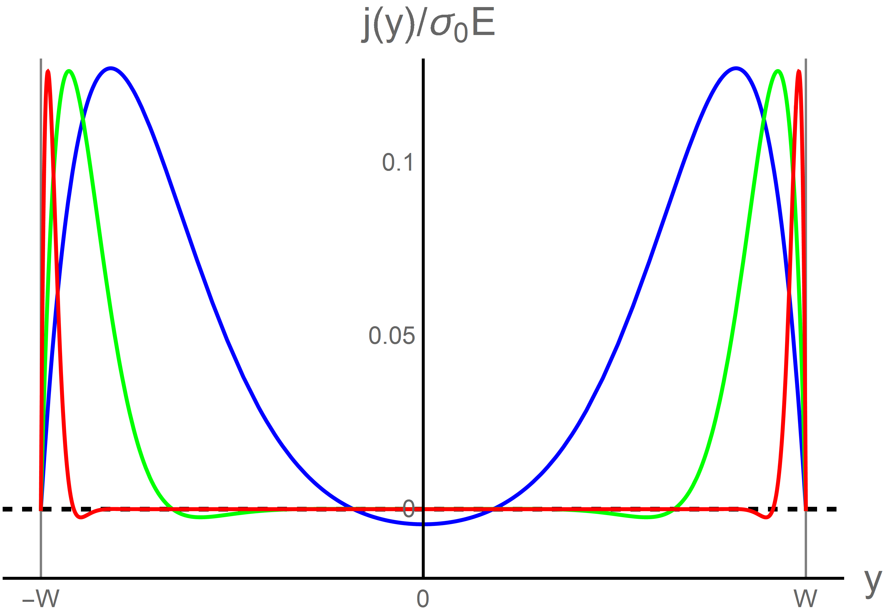
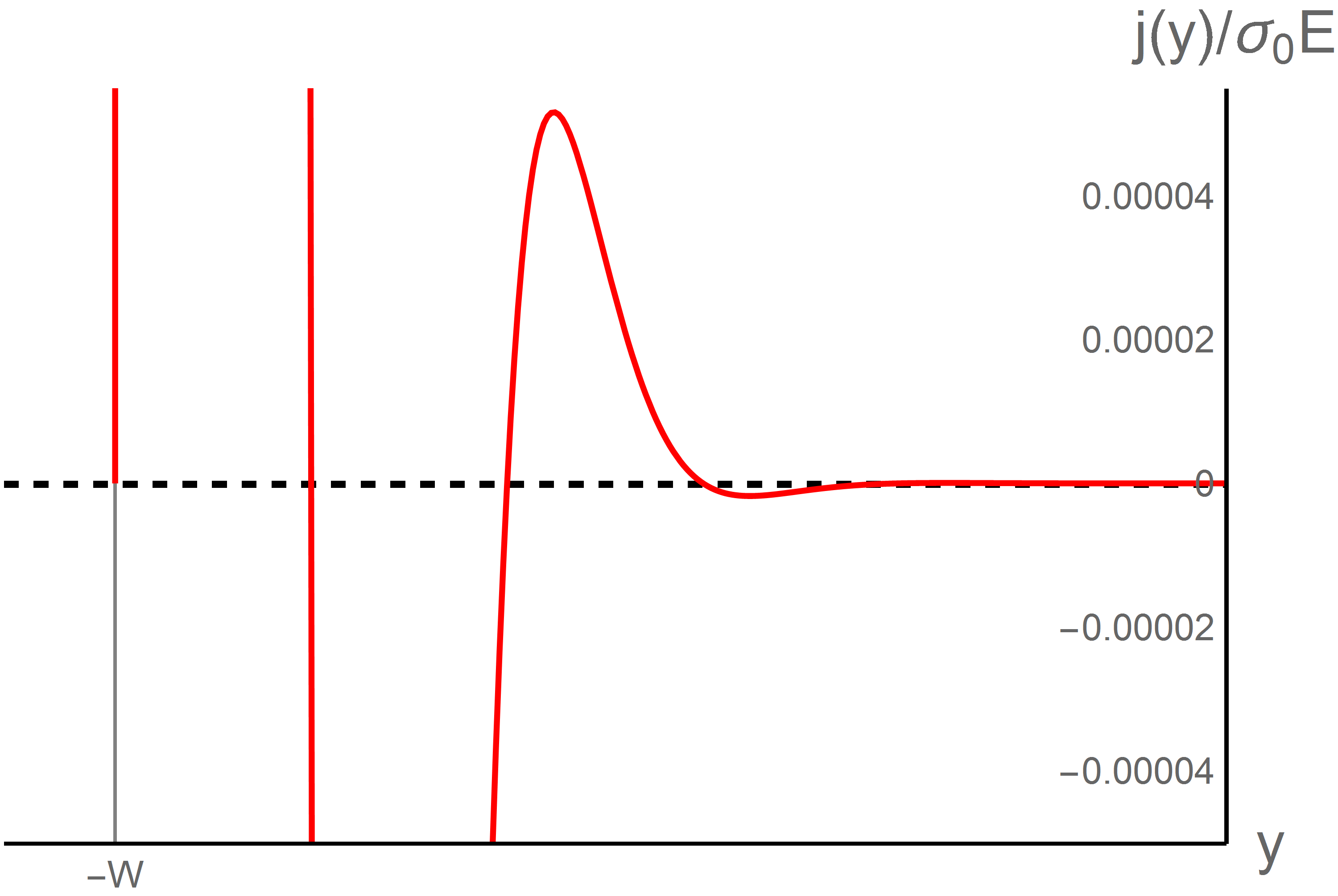
Figure 2: Electric current density (10d) in the regime of fast recombination (16) and strong enough magnetic fields, $B>B_{*}$. Left panel: evolution of the current density with increasing magnetic field. The three curves (blue, green, and red) correspond to ${\omega_{c}\tau_{ee}\!=\!4,10,40}$, respectively, calculated with the values ${\ell_{G}(0)/\ell_{R}\!=\!0.25}$, ${W/\ell_{R}\!=\!0.25}$, and ${\tau\tau_{*}/\tau_{ee}^{2}\!=\!300}$. Right panel: the fine structure of the edge current in strong magnetic field in the narrow range of values near zero. The numerical values correspond to the choice ${\ell_{G}(0)/\ell_{R}\!=\!0.25}$, ${W/\ell_{R}\!=\!0.25}$, ${\tau\tau_{*}/\tau_{ee}^{2}\!=\!1000}$, and ${\omega_{c}\tau_{ee}\!=\!50}$. The vertical grid lines indicate the sample edges and the horizontal dashed line indicates the zero value, ${j\!=\!0}$.

In the absence of the magnetic field the equations (8) decouple and one finds the trivial solution [with the real eigenvalues (10c)]

$$j=\sigma_{0}E\left[1-\frac{\cosh y/\ell_{G}(B)}{\cosh W/[\ell_{G}(B)]}\right],\qquad P=0,$$ (11)

exhibiting the Poiseuille-like flow of the electric current.

II Counterflow of charge carriers in strong magnetic fields

In the presence of the magnetic field, the eigenvalues (10c) may become complex. Indeed, using the relation

$$\ell_{G}(0)\ll\ell_{R},$$

following from combining the assumption $\tau_{ee}\ll\tau_{R}$ [see Eq. (5)] and the fact that $\tau>\tau_{*}$ [by definition (9)], we may re-write the eigenvalues (10c) as

$$\lambda_{\pm}\!\approx\!\frac{1}{2\ell_{G}^{2}(B)}\left[1\!\pm\!\sqrt{\!1\!-\!4\ell_{G}^{2}(B)\ell_{R}^{-2}\omega_{c}^{2}\tau\tau_{*}}\right]\!.$$ (12)

The behavior of the eigenvalues as functions of the magnetic field is controlled by a parameter

$$\xi=\frac{\ell_{G}^{2}(0)}{\ell_{R}^{2}}\frac{\tau\tau_{*}}{\tau_{ee}^{2}}\sim\frac{\tau_{*}^{2}}{\tau_{R}\tau_{ee}}.$$ (13)

As long as $\xi<1$, the eigenvalues, $\lambda_{\pm}$, are real. In Ref. usp, , we have assumed a stronger inequality, $\xi\ll 1$, and explored the resulting magnetoresistance.

II.1 Oscillating currents

Here we are interested in the regime of relatively fast recombination, $\xi>1$. In this case, there exists a particular value of the magnetic field, $B_{*}$, where the expression under the square root in Eq. (12) vanishes:

$$\omega_{c}^{*}=\frac{1}{2\tau_{ee}\sqrt{\xi\!-\!1}}.$$ (14)

For $B>B_{*}$, the eigenvalues (12) are complex,

$$\lambda_{\pm}(B\!>\!B_{*})=\frac{1\pm i\gamma}{2\ell^{2}_{G}(B)},$$ (15a)

where

$$\gamma=\sqrt{\frac{B^{2}\!-\!B_{*}^{2}}{B_{*}^{2}}\frac{1}{1\!+\!4\omega_{c}^{2}\tau_{ee}^{2}}}.$$ (15b)

As a result, the currents (10d) and (10e) acquire an oscillating contribution.

Most interestingly, in the electric current (10d) the oscillation amplitude may exceed the uniform background $j_{0}$ leading to appearance of a counterflow, i.e. a locally negative current density, see Fig. 2. Here we plot the current density (10d) for a case where the sample width is of the same order of magnitude as the Gurzhi length, ${W\sim\ell_{G}(0)}$. In this case, the counterflow first appears in the middle of the sample (see the blue curve in the left panel Fig. 2). As the field is increased, the Gurzhi length $\ell_{G}(B)$ decreases and the current flow is being pushed out towards the sample edges. If the width of the sample is much larger than the Gurzhi length, ${W\gg\ell_{G}(0)}$, then the current is flowing mostly along the edges usp and therefore the counterflow appears in the edge region.

Further analysis is greatly simplified for very strong fields, $B\gg B_{*}$, and in the regime of fast recombination

$$\xi\gg 1\quad\Leftrightarrow\quad\tau_{ee}\ll\tau_{R}\ll\tau_{*}^{2}/\tau_{ee}.$$ (16)

However, in this case there exists an intermediate field range (absent for $\xi\gtrsim 1$)

$$\omega_{c}^{*}\ll\omega_{c}\ll\tau_{ee}^{-1},$$ (17)

such that the imaginary part $\gamma$ exhibits two distinct types of behavior

$$\gamma\approx\begin{cases}B/B_{*},&\omega_{c}^{*}\tau_{ee}\ll\omega_{c}\tau_{ee}\ll 1,\cr\sqrt{\xi},&\omega_{c}\tau_{ee}\gg 1.\end{cases}$$

In both cases the eigenvalues become purely imaginary

$$\lambda_{\pm}(B\gg B_{*})=\pm\,i\ell^{-2}_{c}(B).$$ (18)

As a result, the spatial distribution of the currents is governed by the single field-dependent length scale, $\ell_{c}(B)$:

$$\ell_{c}^{2}(B)=\frac{\ell^{2}_{G}(B)}{\sqrt{\xi}}\begin{cases}(\omega_{c}\tau_{ee})^{-1},&\omega_{c}\tau_{ee}\ll 1,\cr 2,&\omega_{c}\tau_{ee}\gg 1,\end{cases}$$ (19)

$$\qquad\qquad\sim\langle v^{2}\rangle\sqrt{\tau_{R}\tau_{ee}^{3}}\begin{cases}(\omega_{c}\tau_{ee})^{-1},&\omega_{c}\tau_{ee}\ll 1,\cr(\omega_{c}\tau_{ee})^{-2},&\omega_{c}\tau_{ee}\gg 1.\end{cases}$$

Substituting the imaginary eigenvalues (18) into the current density (10d) we find the strongly damped oscillatory behavior illustrated in Fig. 2. When the characteristic scale of the oscillations is much smaller than the width of the system, $\ell_{c}\ll W$, we may expand Eq. (10d) near the sample edges to find the asymptotic expression

$$j(y)\approx\sigma_{0}E\frac{\ell_{c}^{2}(B)}{\ell_{G}^{2}(B)}\sin\left(\frac{W/2\!-\!|y|}{\sqrt{2}\ell_{c}}\right)e^{-\frac{W/2-|y|}{\sqrt{2}\ell_{c}}}.$$ (20)

At the same time, in the middle of the sample the current density is equal to $j_{0}$ (up to exponentially small corrections). In strong magnetic fields, $j_{0}$ is small (in absolutely pure samples it vanishes)

$$j_{0}(B)\approx\sigma_{0}E/(\omega_{c}^{2}\tau\tau_{*})\ll\sigma_{0}E,\qquad j(\tau\!\rightarrow\!\infty)\!=\!0,$$ (21)

such that the bulk current in strong enough magnetic field is almost zero at the scale of the figure. This behavior is illustrated by the red curve in Fig. 2.

The right panel in Fig. 2 illustrates the peculiar structure of the edge current. While in the outermost region, the current is positive, i.e. directed along the external electric field, there is another, inner region carrying negative current flowing in the direction opposite to the electric field. The existence of this region stems from the oscillatory behavior (20). These oscillations, however, are strongly damped by the exponential decay that occurs on the scale that is exactly the oscillation period (in strong enough magnetic field). As a result, already the first minimum of the expression (20) is strongly suppressed leading to the smallness of the negative current seen in Fig. 2. In principle, the bulk current is also oscillating, as illustrated in the right panel in Fig. 2.

II.2 Counterflow threshold

The eigenvalues (10c) remain real in zero field and become complex only for ${B>B_{*}}$. Hence, the counterflow is a threshold phenomenon.

In weak fields the current density is positive everywhere in the system. As the field is increased past $B_{*}$, the current density develops oscillations. The magnitude of the oscillations grows with the field and at some particular field, ${B_{0}>B_{*}}$, the current density reaches zero at some point in the sample, ${j(y_{0};B_{0})=0}$, such that at stronger fields the counterflow is developed around $y_{0}$.

For not too wide samples with ${W\sim\ell_{G}}$ the counterflow appears around ${y_{0}=0}$, see Fig. 2. For wider samples with ${W\gg\ell_{G}}$ the counterflow appears close to the edges, ${|y_{0}|\sim{W}/2}$. In the latter case, both $B_{0}$ and $y_{0}$ can be found analytically in the limit (16). Substituting the eigenvalues (15) into the current density (10d), we find near the edges, i.e. for $|y|\sim W/2$,

$$j=\frac{j_{0}}{\gamma}{\rm Im}\left[\left(1\!-\!e^{\sqrt{1+i\gamma}\frac{|y|-W/2}{\sqrt{2}\ell_{G}(B)}}\right)\left(\frac{1}{2}\!+\!\omega_{c}^{2}\tau\tau_{*}\!+\!i\frac{\gamma}{2}\right)\right].$$

This expression can be simplified as follows. For $\xi\gg 1$, one finds from Eq. (14)

$$\omega_{c}^{*}\tau_{ee}\ll 1\quad\Rightarrow\quad\ell_{G}(B)\approx\ell_{G}(0),\quad\gamma\approx\sqrt{\frac{B^{2}}{B_{*}^{2}}\!-\!1}.$$

Now, denoting

$$\delta=\frac{|y|-W/2}{\sqrt{2}\ell_{G}(B)},\quad\sqrt{1+i\gamma}=c_{1}+ic_{2},$$

we re-write the current density in the form

$$j=\frac{j_{0}}{\gamma}\left[\frac{\gamma}{2}\left(1\!-\!e^{-c_{1}\delta}\cos c_{2}\delta\right)+\omega_{c}^{2}\tau\tau_{*}e^{-c_{1}\delta}\sin c_{2}\delta\right].$$

Since the first term is less than unity, this expression first vanishes at the point ${c_{2}\delta=3\pi/2}$. Substituting this into the current, we find the equation for $\gamma$:

$$\gamma=2\omega_{c}^{2}\tau\tau_{*}e^{-\alpha},\quad\alpha=\frac{3\pi}{2}\frac{c_{1}}{c_{2}}=\frac{3\pi}{2}\frac{1\!+\!\sqrt{1\!+\!\gamma^{2}}}{\gamma},$$

that can be re-written as an equation for ${x=B_{0}/B_{*}>1}$:

$$\sqrt{x^{2}\!-\!1}=x^{2}\frac{\ell_{R}^{2}}{2\ell_{G}^{2}(0)}e^{-\frac{3\pi}{2}\sqrt{\frac{x+1}{x-1}}}.$$

Since ${\ell_{R}/\ell_{G}(0)\gg 1}$, this equation does not admit large solutions ${x\gg 1}$. For ${x\!-\!1\ll 1}$, the equation simplifies to

$$az=e^{z},\quad a=\frac{\ell_{R}^{2}}{6\pi\ell_{G}^{2}(0)},\quad z=\frac{3\pi}{\sqrt{2(x-1)}}.$$

This equation has two solutions for ${a>e}$, out of which we have to choose the solution ${z>1}$ to be consistent with the assumption ${x\!-\!1\ll 1}$. In general, the solutions of the above transcendental equation cannot be expressed in terms of elementary functions. The solution ${z>1}$ is given by the so-called Lambert $W$-function

$$z=-W_{-1}(-1/a).$$

For large $a$, we can use the asymptotic expression

$$z\approx\ln a+\ln\ln a+{\cal O}(1),$$

and as a result

$$B_{0}\approx B_{*}\left[1+\frac{9\pi^{2}}{4(\ln a+\ln\ln a)^{2}}\right].$$

In the extreme case where ${\ln a\gg 1}$, the threshold field $B_{0}$ is rather close to $B_{*}$. Otherwise, ${B_{0}/B_{*}\sim{\cal O}(1)}$.

II.3 Stability analysis

The existence of regions with counterpropagating currents implies the inhomogeneous distribution of the Joule heating across the sample. Indeed, the work done by the external electric field is given by the standard expression ${\boldsymbol{j}(y)\!\cdot\!\boldsymbol{E}}$, which is becomes negative if the direction of the current flow is opposite to that of the field. However, given the smallness of the negative currents, see Eq. (20) and Fig. 2, the overall work of the external electric force is positive, ${IE>0}$. This can be seen either by direct integration of the result (10d), or by using the equations (8) to express the integrated inhomogeneous current density in terms of the integral over the positive definite quadratic form,

$$IE\!=\!\!\int\limits_{-W/2}^{W/2}\!\!dyj(y)E=\frac{1}{\sigma_{0}}\!\!\int\limits_{-W/2}^{W/2}\!\!dy\left[j^{2}(y)\!+\!\ell_{G}^{2}(B)[j^{\prime}(y)]^{2}\right]+\frac{\tau_{*}}{\sigma_{0}\tau}\!\!\int\limits_{-W/2}^{W/2}\!\!dy\left[P^{2}(y)\!+\!\ell^{2}_{R}[P^{\prime}(y)]^{2}\right],$$ (22)

which demonstrates the positivity of the work $IE$ irrespective to the particular form of the solution $j(y)$. Hence, the system does not develop any instability (in contrast to the case of the Ohmic regime with negative conductivity zrs ). The fact that in some part of the sample the local Joule heating appears to be negative means that the heat is being redistributed between different parts of the electronic system. This process is accompanied by a lateral energy flow. The corresponding energy current can be determined by solving the nonlinear hydrodynamic equations (taking into account the Joule’s heat). This calculation is beyond the scope of the present paper and will be reported elsewhere.

Similar arguments can be used to establish the stability of the solution (10d) while allowing for charge fluctuations. Following the standard procedure for stability analysis dau6 , we introduce plane wave solutions in the form

$${\cal O}(x,y;t)\rightarrow{\cal O}(x,y)e^{i\omega t},$$

for fluctuations of all currents and densities in Eqs. (1), (2) including the fluctuation of the charge density ${\delta{n}=n-n^{(0)}}$ (${n=n_{h}-n_{e}}$). These fluctuations induce an electric field (the Vlasov field dau10 ). In the simplest case of a gated 2D sample in the limit of strong screening us2 , the induced field is proportional to the gradient of the charge density fluctuation, $\boldsymbol{E}_{V}=-(4\pi ed/\epsilon)\boldsymbol{\nabla}\delta n$, where $d$ is the distance to the gate and $\epsilon$ is the dielectric constant. The dependence on $x$ is dictated by the geometry of the problem and is given by $e^{ik_{x}x}$. The eigenmode frequency $\omega=\omega_{l}(k_{x})$ has to be determined by solving Eqs. (1), (2) and can in principle be complex. Stability of a given solution is determined by the sign of the imaginary part of the frequency with stable solutions corresponding to ${\rm Im}\;\omega_{l}(k_{x})\geqslant 0$. Substituting the above Ansatz into Eqs. (1), (2), we follow the same steps leading to Eqs. (6), (8). As a result, we arrive at the following equations for the amplitudes of the current densities:

$$i\omega\boldsymbol{P}=-\boldsymbol{P}/\tau+\omega_{c}\left[\boldsymbol{j}\times\boldsymbol{e}_{z}\right]+\eta_{xx}\Delta\boldsymbol{P}+\frac{\langle v^{2}\rangle}{2}\frac{1}{i\omega+1/\tau_{R}}\boldsymbol{\nabla}(\boldsymbol{\nabla}\!\cdot\!\boldsymbol{P}),$$ (23a)

$$i\omega\boldsymbol{j}=-\boldsymbol{j}/\tau_{*}+\omega_{c}\left[\boldsymbol{P}\times\boldsymbol{e}_{z}\right]+\eta_{xx}\Delta\boldsymbol{j}+\frac{s^{2}}{i\omega}\boldsymbol{\nabla}(\boldsymbol{\nabla}\!\cdot\!\boldsymbol{j}),\qquad s^{2}=\frac{\langle v^{2}\rangle}{2}+\frac{4\pi e^{2}}{m\epsilon}\rho^{(0)}d.$$ (23b)

The quantities in Eqs. (23) are fluctuations around the time-independent (steady state) solution and hence the external electric field does not enter Eqs. (23). As a result, we have a system of homogeneous linear equations which has nontrivial solutions only if the determinant of the system is equal to zero. The latter equation yields the allowed frequencies $\omega_{l}(k_{x})$. Our goal, however, is more modest – we just need to establish the sign of ${{\rm{Im}}\;\omega_{l}(k_{x})}$. To that end, we multiply Eq. (23a) by $\boldsymbol{P}^{*}$, take a complex conjugate of Eq. (23b) and multiply by $\boldsymbol{j}$, then add the resulting equations and integrate over the area of the sample. As a result we find the following relation:

$$i\omega\!\int\!dxdy|\boldsymbol{P}|^{2}-i\omega^{*}\!\int\!dxdy|\boldsymbol{j}|^{2}=-\frac{1}{\tau}\!\int\!dxdy|\boldsymbol{P}|^{2}-\frac{1}{\tau_{*}}\!\int\!dxdy|\boldsymbol{j}|^{2}+\eta_{xx}\!\int\!dxdy\left(\boldsymbol{P}^{*}\Delta\boldsymbol{P}+\boldsymbol{j}\Delta\boldsymbol{j}^{*}\right)$$

$$\quad\qquad\qquad\qquad\qquad\qquad\qquad\qquad+\frac{\langle v^{2}\rangle}{2}\frac{1}{i\omega+1/\tau_{R}}\!\int\!dxdy\boldsymbol{P}^{*}\!\cdot\!\boldsymbol{\nabla}(\boldsymbol{\nabla}\!\cdot\!\boldsymbol{P})-\frac{s^{2}}{i\omega}\!\int\!dxdy\boldsymbol{j}\!\cdot\!\boldsymbol{\nabla}(\boldsymbol{\nabla}\!\cdot\!\boldsymbol{j}^{*}).$$ (24)

The last three terms can now be integrated by parts with the boundary terms vanishing due to the no-slip boundary conditions, e.g.

$$\int\!dxdy\boldsymbol{P}^{*}\!\cdot\!\boldsymbol{\nabla}(\boldsymbol{\nabla}\!\cdot\!\boldsymbol{P})=\int\!dxdy|\boldsymbol{\nabla}\!\cdot\!\boldsymbol{P}|^{2}.$$

After that the only complex quantity in the equation is the frequency. Introducing its real and imaginary parts, ${\omega=\omega_{1}+i\omega_{2}}$, we can separate the real part of the equation and find the relation

$$\omega_{2}\!\int\!dxdy\left[|\boldsymbol{P}|^{2}+|\boldsymbol{j}|^{2}+\frac{s^{2}}{\omega_{1}^{2}+\omega_{2}^{2}}|\boldsymbol{\nabla}\!\cdot\!\boldsymbol{j}|^{2}+\frac{\langle v^{2}\rangle}{2}\frac{|\boldsymbol{\nabla}\!\cdot\!\boldsymbol{P}|^{2}}{\omega_{1}^{2}+(\omega_{2}-1/\tau_{R})^{2}}\right]=\frac{1}{\tau}\!\int\!dxdy|\boldsymbol{P}|^{2}+\frac{1}{\tau_{*}}\!\int\!dxdy|\boldsymbol{j}|^{2}$$

$$\quad\qquad\qquad\quad\qquad\qquad+\eta_{xx}\!\int\!dxdy\sum_{\alpha=x,y}\left(|\boldsymbol{\nabla}P_{\alpha}|^{2}+|\boldsymbol{\nabla}j_{\alpha}|^{2}\right)+\frac{\langle v^{2}\rangle}{2\tau_{R}}\frac{1}{\omega_{1}^{2}+(\omega_{2}-1/\tau_{R})^{2}}\int\!dxdy|\boldsymbol{\nabla}\!\cdot\!\boldsymbol{P}|^{2}.$$ (25)

Given that every single term in Eq. (II.3) is manifestly positive, we conclude that for every possible solution of the linear system (23)

$$\omega_{2}={\rm Im}\;\omega_{l}(k_{x})>0,$$ (26)

proving the stability of our theory. Note that this conclusion is independent of the values of $\tau$ and $\tau_{eh}$ and remains valid even in the limit $\tau,\tau_{eh}\rightarrow\infty$.

III Magnetoresistance

Integrating the current density (10d) over $y$, we find the total current, $I$, and hence the sample resistance usp , $R$:

$$R\!=\!\frac{R_{0}(\lambda_{+}\!-\!\lambda_{-})}{\left[1\!-\!\frac{2\tanh\left(\sqrt{\lambda_{+}}W/2\right)}{W\sqrt{\lambda_{+}}}\right]\left[\ell_{G}^{-2}(B)\!-\!\frac{\lambda_{-}}{1+\omega_{c}^{2}\tau\tau_{*}}\right]\!-\!\left[1\!-\!\frac{2\tanh\left(\sqrt{\lambda_{-}}W/2\right)}{W\sqrt{\lambda_{-}}}\right]\left[\ell_{G}^{-2}(B)\!-\!\frac{\lambda_{+}}{1+\omega_{c}^{2}\tau\tau_{*}}\right]},\qquad R_{0}\!=\!\frac{L}{e\sigma_{0}W}.$$ (27)

The general expression (27) for the sample resistance was analyzed in Ref. usp, in the case of weak recombination with the real eigenvalues (10c). Here we focus on the opposite case of strong recombination, where $\lambda_{\pm}$ may take the complex values (15). The result is illustrated in Figs. 3 and 4, where we show the dependence of the sample resistance on the external magnetic field.

III.1 Negative magnetoresistance

In Fig. 3 we illustrate the regime of negative magnetoresistance similar to that discussed in Ref. usp, . In weak fields, the eigenvalues (10c) remain real and the resistance (27) decreases parabolically usp . For the choice of parameter values in Fig. 3, i.e. $W\leqslant\ell_{G}(0)$, the parabolic field dependence is given by usp

$$R(B\rightarrow 0)/R(0)=1-4\omega_{c}^{2}\tau_{ee}^{2}.$$ (28a)

This behavior is shown in Fig. 3 by the green dashed line.

In strong fields, the resistance grows linearly (i.e. the magnetoresistance is positive). Similarly to the results of Ref. usp, , we find (for ${\omega_{c}\tau_{ee}\gg{\rm max}[1,\ell_{G}(0)/(W\sqrt{\xi})]}$)

$$R\approx R_{0}A\left[\omega_{c}\tau_{ee}\!-\!A\frac{\tau_{ee}^{2}}{\tau\tau_{*}}\right],$$ (28b)

where

$$A=-i\frac{W\gamma}{\ell_{G}(0)\sqrt{2}}\left[\frac{1}{\sqrt{1\!+\!i\gamma}}\!-\!\frac{1}{\sqrt{1\!-\!i\gamma}}\right]^{-1}.$$ (28c)

This behavior is shown in Fig. 3 by the blue dashed line. In the limit (16), i.e. for $\gamma\rightarrow\infty$, the coefficient $A$ simplifies to

$$A(\gamma\rightarrow\infty)\approx\frac{W\xi^{3/4}}{2\ell_{G}(0)}.$$ (28d)

III.2 Intermediate power-law regime

In Fig. 4 we illustrate the regime of positive magnetoresistance focusing on the limit (16). In this case, in addition to the parabolic and linear asymptotics (in weak and strong fields, respectively) discussed in Ref. usp, , we find an additional regime appearing in the intermediate field range (17).

For the parameter values used in Fig. 4, ${\ell_{R}\gg{W}>W_{0}}$ (where ${W_{0}\approx[48\ell_{R}^{2}\ell_{G}(0)\tau_{ee}^{2}/(\tau\tau_{*})]^{1/3}}$ is the width where magnetoresistance changes sign), the parabolic dependence of the resistance in the weakest fields is usp

$$\frac{R(B\rightarrow 0)}{R(0)}=1+A_{1}\omega_{c}^{2}\tau_{ee}^{2},\qquad A_{1}=\frac{W^{2}}{12\ell_{R}^{2}}\frac{\tau\tau_{*}}{\tau_{ee}^{2}}.$$ (29)

This behavior is shown in Fig. 4 by the green dashed line and is a good approximation only in the very weak fields, $B<B_{*}$, see the upper inset. In stronger fields the eigenvalues (10c) become complex.

In the strongest fields, the resistance (27) recovers the linear behavior (28b) shown in Fig. 4 by the blue dashed line.

In the intermediate field range (17), the eigenvalues (10c) are linear in $B$, see Eq. (19). Then, for wide enough samples, ${W\gg\ell_{c}(B)}$, the field dependence of the resistance (27) is dominated by the power law with the exponent $3/2$:

$$\frac{R(B)}{R_{0}W}\approx\frac{\sqrt{\ell_{G}(0)}}{\sqrt{2}\ell_{R}^{3/2}}(\tau\tau_{*})^{3/4}\omega_{c}^{3/2},$$ (30)

shown in Fig. 4 by the black dashed line. This behavior appears only in the limit (16) of very strong recombination. For weaker recombination, $\xi>1$, the field range (17) does not exist, the eigenvalues (10c) do not develop the linear behavior, and as a result the power law $R\sim B^{3/2}$ does not appear.

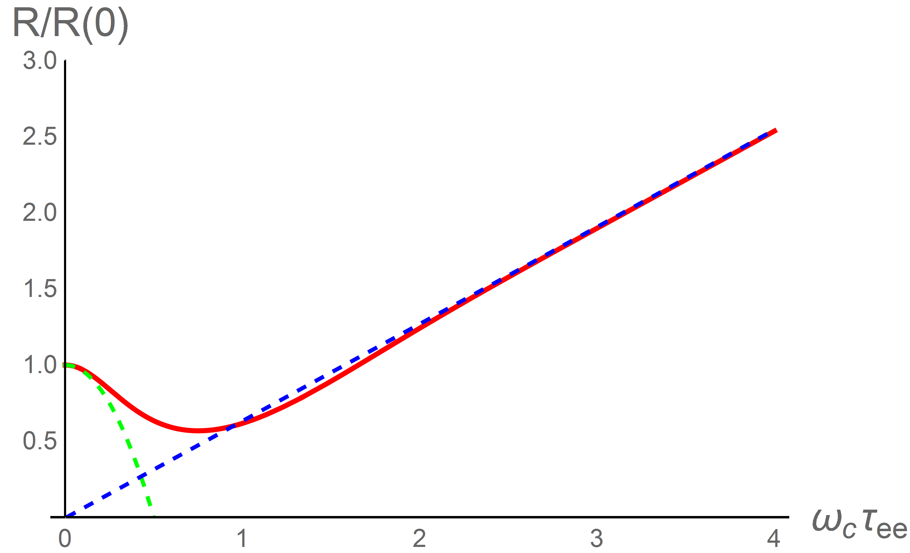
Figure 3: Sample resistance (27) as a function of the magnetic field. The numerical values correspond to the following choice of parameters: ${\ell_{G}(0)/\ell_{R}\!=\!0.2}$, ${W/\ell_{R}\!=\!0.2}$, ${\tau\tau_{*}/\tau_{ee}^{2}\!=\!1000}$. The green dashed line indicates the negative, parabolic magnetoresistance in weak fields usp , see Eq. (28a). The blue dashed line shows the positive, linear magnetoresistance (28b).

IV Qualitative discussion

The nonuniform current distribution discussed in this paper bears a certain similarity to the nonuniform spin density near a surface of a three-dimensional semiconductor sample spin . In that case, the inhomogeneous spin density is created optically at the surface and then propagates into the bulk of the sample by mans of carrier diffusion. The equations of the spin diffusion in magnetic field derived in Ref. spin, are similar to Eqs. (8) if one neglects electron-hole and disorder scattering. The resulting spin density shows an inhomogeneity similar to that in Eq. (20) exhibiting oscillating behavior near the surface that decays into the bulk of the sample.

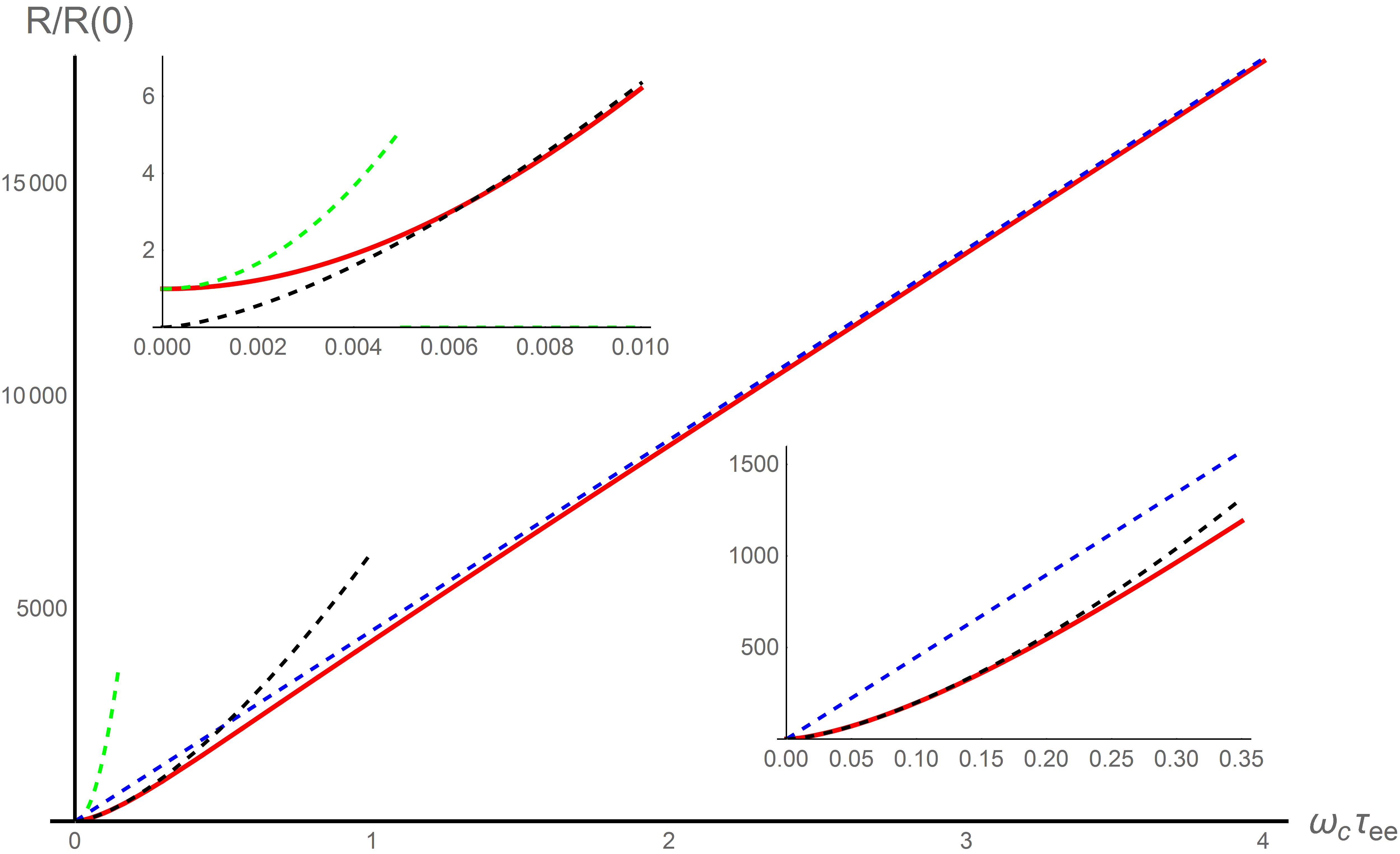
Figure 4: Sample resistance (27) as a function of the magnetic field for ${\ell_{G}(0)/\ell_{R}\!=\!0.005}$, ${W/\ell_{R}\!=\!0.01}$, ${\tau\tau_{*}/\tau_{ee}^{2}\!=\!10^{10}}$. The dashed lines indicate the three asymptotic regimes: parabolic (green), Eq. (29); linear (blue), Eq. (28b); and the power law, $R\sim B^{3/2}$, (black) Eq. (30). The insets zoom into the range of weak (up) and intermediate (down) fields.

Physically, the counterflow in compensated semimetals appears due to the influence of the strong magnetic field on the motion of charge carriers. A non-quantized magnetic field tends to bend semicalssical trajectories away from the direction of the applied electric field. In the context of an inviscid two-component system (e.g., a nearly compensated semimetal) this effect was discussed in Ref. us3, . Taking into account viscous effects, we find that away from the boundary electrons and holes follow nontrivial trajectories illustrated in Fig. 5.

In strong magnetic fields (bottom panels in Fig. 5), both electrons and holes in the bulk of the sample are moving across the sample such that the the combined electric current nearly vanishes, see Eq. (21), while the quasiparticle current $\boldsymbol{P}$ is nearly uniform. This is consistent with earlier discussions of the effect of non-quantizing magnetic field on graphene meg ; usg or compensated semimetals us2 ; us3 ; vas and should be contrasted with the usual interpretation of the classical Hall effect in single-component electronic systems. In the latter case, the lateral electric current which would be induced by the magnetic field in an infinite system is compensated by the Hall voltage and as a result, electrons move only in the direction of the applied electric field. In a two-component system at charge neutrality the Hall voltage is absent so that the electric currents in the two constituent subsystems have to cancel each other.

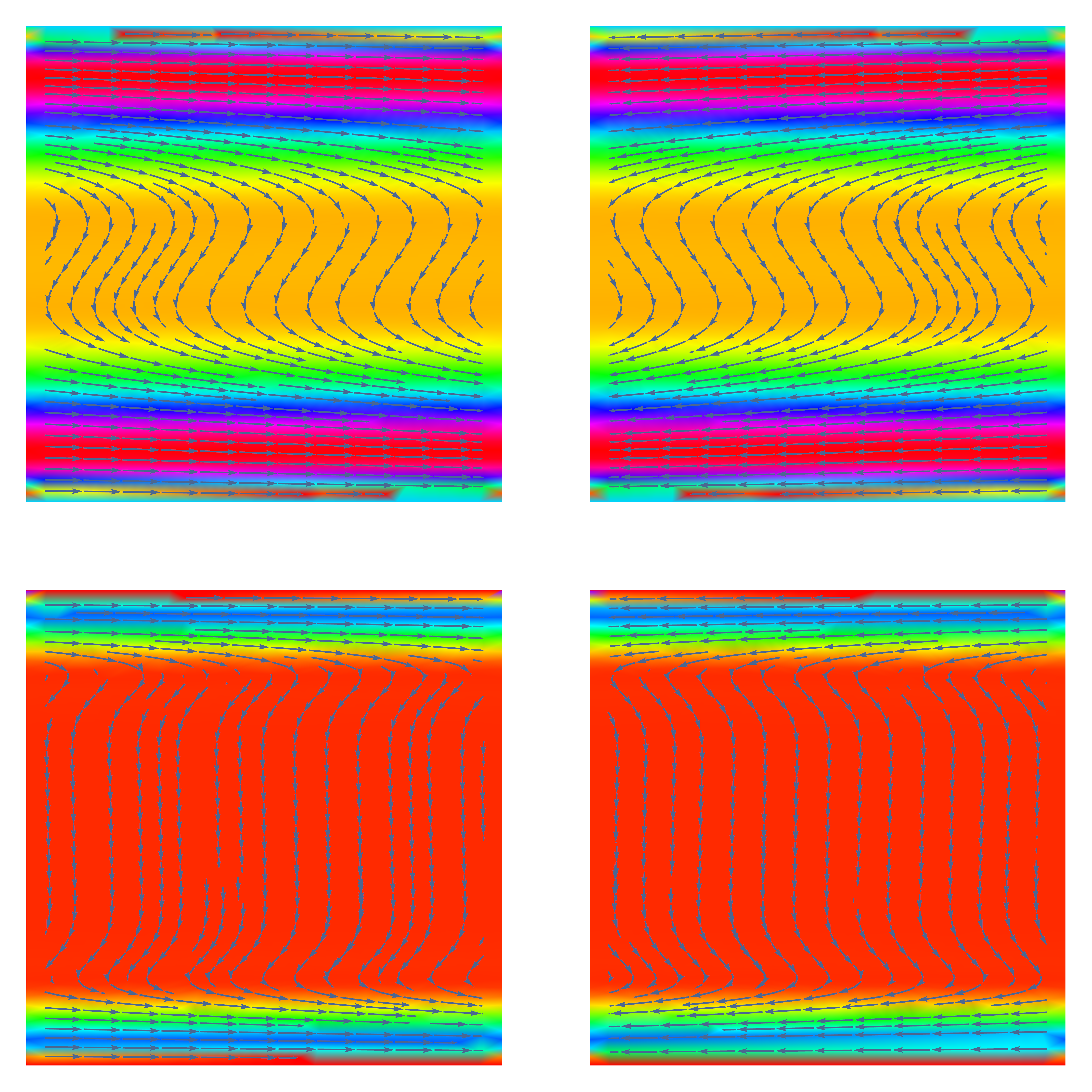
Figure 5: Individual electron (left) and hole (right) flows. The numerical values correspond to the same choice of parameters as in Fig. 2: ${\ell_{G}(0)/\ell_{R}\!=\!0.25}$, ${W/\ell_{R}\!=\!0.25}$, ${\tau\tau_{*}/\tau_{ee}^{2}\!=\!300}$. The top panels show data for ${\omega_{c}\tau_{ee}\!=\!4}$ (same as the blue curve in the left panel in Fig 2), the bottom panels show data for ${\omega_{c}\tau_{ee}\!=\!10}$ (same as the green curve in the left panel in Fig 2).

In the edge region, the electron and hole currents experience a rotation: very close to the edge [within the distance of the order of the Gurzhi length $\ell_{G}(B)$], the charge carriers move along the boundary, while in the next layer (controlled by the quasiparticle recombination) the lateral component of the currents appears. As a result, the current vectors exhibit an intricate rotation pattern: first they overshoot the angle $\pi/2$ between the edge and bulk flows, but never reaching the angle $\pi$ and eventually return to $\pi/2$. This relatively complex pattern is on one hand, required by vanishing quasiparticle current $\boldsymbol{P}$ at the edge, but on the other hand, appears due to the presence of the viscous layer. In an inviscid system us2 ; us3 , there is no zero boundary condition on the tangential component of the electric current and hence the electron and hole currents rotate smoothly with their angle relative to the boundary varying from $0$ to $\pi/2$.

In weaker fields, the above rotation pattern is incomplete due to the overlap of the two boundary regions (i.e. ${\ell_{c}\sim{W}}$). In this case the pronounced bulk region with the transverse moving charge carriers does not develop, see the top panels in Fig. 5. As a result, the counterflow occupies not the edge, but a central region of the sample.

The nonuniform (and rotating) flows of electrons and holes are characterized by the non-vanishing $\boldsymbol{\nabla}\!\times\!\boldsymbol{j}_{e(h)}$. This should not be confused with the true vorticity in the sense of a whirlpool (or eddy) formation exg1 ; fal . In fact, already the standard Poiseuille flow dau6 ; poi possess the nonvanishing $\boldsymbol{\nabla}\!\times\!\boldsymbol{v}$ (where $\boldsymbol{v}$ is the hydrodynamic velocity). However, the Poiseuille flow is incompressible with $\boldsymbol{\nabla}\!\cdot\!\boldsymbol{v}\!=\!0$. As a result, the transverse component of the velocity vanishes exactly, $v_{y}=0$, and neither the true vorticity, nor any other rotation of the velocity vector may appear. If the fluid exhibiting the Poiseuille flow is charged (e.g., in a plasma with heavy ions that provide the effective positive background to the electronic fluid), then the vanishing of the transverse velocity component is ensured by the Hall voltage. Now, in the two-component system with quasiparticle recombination both the electron and hole fluids are compressible, $\boldsymbol{\nabla}\!\cdot\!\boldsymbol{j}_{e(h)}\neq 0$, with the total electric current fulfilling $\boldsymbol{\nabla}\!\cdot\!\boldsymbol{j}=0$ (due to charge conservation). In this case, the electron and hole currents exhibit the rotation shown in Fig. 5, which is the ultimate reason for the oscillating behavior (20).

V Summary

To summarize, we have considered the viscous electronic flow in compensated semimetals with strong quasiparticle recombination and in confined geometries. While the sample resistance is qualitatively similar to the case of weak recombination considered in Ref. usp, , see Fig. 3, the current density profile shows a qualitatively different behavior. The current is flowing mostly (with exponential accuracy) along the sample edges. At each edge, the current flow is nonuniform and consists of two counterpropagating stripes, see Figs. 1 and 2. Such counterflows are expected to be more general than the particular problem considered in this paper and may appear even in single-component electron fluids either in the ac transport moe ; aac or in the thermoelectric flow usf .

The appearance of the small local current density in the direction opposite to that of the applied electric field does not affect the global thermoelectric properties of the sample. However, this is a direct indication of the inhomogeneous distribution of the Joule heating across the sample accompanied by a lateral energy flow. As the effect of Joule heating is beyond linear response, a proper theory of the thermoelectric phenomena in semimetals requires a solution of the nonlinear hydrodynamic equations. Such a theory will be reported elsewhere.

- (1) D. A. Bandurin, I. Torre, R. Krishna Kumar, M. Ben Shalom, A. Tomadin, A. Principi, G. H. Auton, E. Khestanova, K. S. Novoselov, I. V. Grigorieva, L. A. Ponomarenko, A. K. Geim, and M. Polini, Science 351, 1055 (2016).
- (2) J. Crossno, J.K. Shi, K. Wang, X. Liu, A. Harzheim, A. Lucas, S. Sachdev, P. Kim, T. Taniguchi, K. Watanabe, T.A. Ohki, and K.C. Fong, Science 351, 1058 (2016).
- (3) R. Krishna Kumar, D. A. Bandurin, F. M. D. Pellegrino, Y. Cao, A. Principi, H. Guo, G. H. Auton, M. Ben Shalom, L. A. Ponomarenko, G. Falkovich, K.Watanabe, T. Taniguchi, I. V. Grigorieva, L. S. Levitov, M. Polini, and A. K. Geim, Nature Physics 13, 1182 (2017).
- (4) P.J.W. Moll, P. Kushwaha, N. Nandi, B. Schmidt, and A.P. Mackenzie, Science 351, 1061 (2016).
- (5) J. Gooth, F. Menges, C. Shekhar, V. Süß, N. Kumar, Y. Sun, U. Drechsler, R. Zierold, C. Felser, and B. Gotsmann, arXiv:1706.05925 (2017).
- (6) B. N. Narozhny, I. V. Gornyi, A D. Mirlin, and J. Schmalian, Annalen der Physik 529, 1700043 (2017).
- (7) A. Lucas and K. C. Fong, J. Phys.: Cond. Mat. 30, 053001 (2018).
- (8) Y. Nam, D.-K. Ki, D. Soler-Delgado, and A. F. Morpurgo, Nature Phys. 13,1207 (2017).
- (9) H. Guo, E. Ilseven, G. Falkovich, and L. S. Levitov, PNAS 114, 3068 (2017).
- (10) L. S. Levitov and G. Falkovich, Nature Physics 12, 672 (2016).
- (11) G. M. Gusev, A. D. Levin, E. V. Levinson, and A. K. Bakarov, AIP Advances 8, 025318 (2018).
- (12) P.S. Alekseev, Phys. Rev. Lett. 117, 166601 (2016).
- (13) T. Scaffidi, N. Nandi, B. Schmidt, A. P. Mackenzie, and J. E. Moore, Phys. Rev. Lett. 118, 226601 (2017).
- (14) P. S. Alekseev, M. A. Semina, arXiv:1801.02879 (2018).
- (15) P. S. Alekseev, A. P. Dmitriev, I. V. Gornyi, V. Y. Kachorovskii, B. N. Narozhny, and M. Titov, Phys. Rev. B 97, 085109 (2018).
- (16) L. D. Landau and E. M. Lifshitz, Fluid Mechanics (Butterworth-Heinemann, Oxford, UK, 2000).
- (17) U. Briskot, M. Schütt, I. V. Gornyi, M. Titov, B. N. Narozhny, and A. D. Mirlin, Phys. Rev. B 92, 115426 (2015).
- (18) J. L. M. Poiseuille, C. R. Acad. Sci. 11, 961 (1840).
- (19) P. S. Alekseev, A. P. Dmitriev, I. V. Gornyi, V. Y. Kachorovskii, B. N. Narozhny, M. Schütt, and M. Titov, Phys. Rev. Lett. 114, 156601 (2015).
- (20) P. S. Alekseev, A. P. Dmitriev, I. V. Gornyi, V. Y. Kachorovskii, B. N. Narozhny, M. Schütt, and M. Titov, Phys. Rev. B 95, 165410 (2017).
- (21) M. Titov, R. V. Gorbachev, B. N. Narozhny, T. Tudorovskiy, M. Schütt, P. M. Ostrovsky, I. V. Gornyi, A. D. Mirlin, M. I. Katsnelson, K. S. Novoselov, A. K. Geim, and L. A. Ponomarenko, Phys. Rev. Lett. 111, 166601 (2013).
- (22) G. M. Gusev, E. B. Olshanetsky, Z. D. Kvon, N. N. Mikhailov, and S. A. Dvoretsky, Phys. Rev. B 87, 081311 (2013).
- (23) S. Wiedmann, A. Jost, C. Thienel, C. Brune, P. Leubner, H. Buhmann, L. W. Molenkamp, J. C. Maan, and U. Zeitler, Phys. Rev. B 91, 205311 (2015).
- (24) G. Yu. Vasileva, D. Smirnov, Yu. L. Ivanov, Yu. B. Vasilyev, P. S. Alekseev, A. P. Dmitriev, I. V. Gornyi, V. Yu. Kachorovskii, M. Titov, B. N. Narozhny, and R. J. Haug, Phys. Rev. B 93, 195430 (2016).
- (25) R. Moessner, P. Surowka, and P. Witkowski, Phys. Rev. B 97, 161112(R) (2018).
- (26) P. S. Alekseev, arXiv:1802.09179 (2018).
- (27) P. S. Alekseev, A. P. Dmitriev, I. V. Gornyi, V. Y. Kachorovskii, B. N. Narozhny, and M. Titov, to be published.
- (28) B. N. Narozhny, I. V. Gornyi, M. Titov, M. Schütt, and A. D. Mirlin, Phys. Rev. B 91, 035414 (2015).
- (29) J.M. Link, B.N. Narozhny, E.I. Kiselev, and J. Schmalian, Phys. Rev. Lett. 120, 196801 (2018).
- (30) M. S. Steinberg, Phys. Rev. 109, 1486 (1958).
- (31) D. Svintsov, Phys. Rev. B 97, 121405(R) (2018).
- (32) I. A. Dmitriev, A. D. Mirlin, D. G. Polyakov, and M. A. Zudov, Rev. Mod. Phys. 84, 1709 (2012).
- (33) E. M. Lifshitz and L. P. Pitaevskii, Physical Kinetics (Butterworth-Heinemann, Oxford, UK, 1981).
- (34) R. I. Dzhioev, B. P. Zakharchenya, V. L. Korenev, and M. N. Stepanova, Fiz. Tverd. Tela (St. Petersburg) 39, 1975 (1997) [Phys. Solid State 39, 1765 (1997)].