The formation of extremely diffuse galaxy cores
by merging supermassive black holes

Abstract

Given its velocity dispersion, the early-type galaxy NGC 1600 has an unusually massive ($M_{\bullet}=1.7\times 10^{10}M_{\odot}$) central supermassive black hole (SMBH), surrounded by a large core ($r_{\mathrm{b}}=0.7$ kpc) with a tangentially biased stellar distribution. We present high-resolution equal-mass merger simulations including SMBHs to study the formation of such systems. The structural parameters of the progenitor ellipticals were chosen to produce merger remnants resembling NGC 1600. We test initial stellar density slopes of $\rho\propto r^{-1}$ and $\rho\propto r^{-3/2}$ and vary the initial SMBH masses from $8.5\times 10^{8}$ to $8.5\times 10^{9}$ $M_{\odot}$. With increasing SMBH mass the merger remnants show a systematic decrease in central surface brightness, an increasing core size, and an increasingly tangentially biased central velocity anisotropy. Two-dimensional kinematic maps reveal decoupled, rotating core regions for the most massive SMBHs. The stellar cores form rapidly as the SMBHs become bound, while the velocity anisotropy develops more slowly after the SMBH binaries become hard. The simulated merger remnants follow distinct relations between the core radius and the sphere-of-influence, and the SMBH mass, similar to observed systems. We find a systematic change in the relations as a function of the progenitor density slope, and present a simple scouring model reproducing this behavior. Finally, we find the best agreement with NGC 1600 using SMBH masses totaling the observed value of $M_{\bullet}=1.7\times 10^{10}M_{\odot}$. In general, density slopes of $\rho\propto r^{-3/2}$ for the progenitor galaxies are strongly favored for the equal-mass merger scenario.

1 Introduction

Observations have revealed a dichotomy in the population of bright elliptical galaxies, with the brighter ellipticals $(M_{B}\lesssim-20.5)$ being dominated by systems with little rotation (slow-rotators), typically boxy isophotes and relatively shallow central surface brightness profiles, whereas intermediate luminosity ellipticals $(-20.5\lesssim M_{B}\lesssim-18.5)$ have more rotational support (fast-rotators), more disky isophotes and steeper power-law like central surface brightness profiles (e.g. Kormendy & Bender 1996; Faber et al. 1997).

These morphological differences are also indicative of two distinct formation paths for early-type galaxies. Lower luminosity elliptical galaxies likely formed through in-situ star formation and mergers of gas-rich disk-dominated galaxies, with the accompanying merger induced star-burst resulting in cuspy central stellar profiles (e.g. Barnes & Hernquist 1996; Naab & Trujillo 2006; Cappellari et al. 2007; Hopkins et al. 2008; Johansson et al. 2009b; Krajnović et al. 2011; Cappellari 2016; Lahén et al. 2018). The more massive early-type galaxies are instead believed to have assembled through a two-stage process, in which the early assembly is dominated by rapid in situ star formation fueled by cold gas flows and hierarchical merging of multiple star-bursting progenitors, whereas the later growth below redshifts of $z\lesssim 2-3$ is dominated by a more quiescent phase of gas-poor (dry) merging, in which the galaxy accretes stars formed mainly in progenitors outside the main galaxy (e.g. Naab et al. 2009; Oser et al. 2010; Feldmann et al. 2011; Johansson et al. 2009c, 2012; Moster et al. 2013; Wellons et al. 2015; Rodriguez-Gomez et al. 2016, see also Naab & Ostriker 2017 for a review).

In general the smooth light profiles of elliptical galaxies over several orders of magnitude in radius are well described by a single three-parameter Sérsic profile (Sérsic, 1963; Caon et al., 1993). However, the most massive ellipticals often exhibit in their central light profiles significantly flatter regions of missing light, when compared to the inwards extrapolation of the outer Sérsic profile. The radius at which this departure from the Sérsic profile occurs is often called the ”break” or ”core” radius, denoted by $r_{\mathrm{b}}$. Typically the size of the core region is $r_{\mathrm{b}}\sim 50-500\ \rm pc$ (e.g. Ravindranath et al. 2002; Lauer et al. 2007; Rusli et al. 2013a; Dullo & Graham 2014), but in extreme cases the core can extend beyond the kpc-scale (e.g. Postman et al. 2012; López-Cruz et al. 2014; Dullo et al. 2017).

At face value the existence of cores in massive galaxies poses a theoretical challenge to their formation scenario. The reason for this is that the central structure of a merger remnant without gas is dominated by the more concentrated of the two progenitors, meaning that the steeper central density cusp survives (e.g. Holley-Bockelmann & Richstone 1999; Boylan-Kolchin & Ma 2004a). The massive ellipticals are believed to have been assembled from mergers of lower-mass ellipticals with steep central-density cusps at high redshifts. Situations in which the merger progenitors contain gas complicate the problem, as the angular momentum transfer in a merger leads to gas inflows that trigger central starbursts, resulting in the formation of even denser central regions (e.g. Barnes & Hernquist 1991). Thus the shallow cores widely observed in massive early-type galaxies must result from another physical process than galaxy merging.

The supermassive black holes (SMBHs) found in the centers of all massive galaxies in the local Universe (e.g. Kormendy & Richstone 1995; Ferrarese & Ford 2005; Kormendy & Ho 2013) could potentially provide a core formation mechanism. In particular, there is evidence for a co-evolution of SMBHs and their host galaxies as manifested in the surprisingly tight relations between the SMBH masses and the fundamental properties of the galactic bulges that host them, e.g. the bulge mass (e.g. Häring & Rix 2004) and the bulge stellar velocity dispersion (e.g. Ferrarese & Merritt 2000; Gebhardt et al. 2000; Tremaine et al. 2002). In addition there are also indications for a core-black hole mass relation as the size of the core and the amount of ”missing” starlight in the center of the core galaxy approximately scale with the mass of the central black hole (Graham, 2004; de Ruiter et al., 2005; Lauer et al., 2007; Kormendy & Bender, 2009; Rusli et al., 2013a; Dullo & Graham, 2014; Thomas et al., 2016).

The formation process of cores in massive elliptical galaxies is commonly attributed to core scouring by SMBH binaries in the aftermath of galaxy mergers. After sinking to the center of the merger remnant by dynamical friction (Chandrasekhar, 1943) from surrounding stars and dark matter, the two SMBHs form a gravitationally bound binary. The binary subsequently shrinks by interacting with the stellar background and ejecting stars in complex three-body interactions, which carry away energy and angular momentum from the SMBH binary system (e.g. Hills & Fullerton 1980). The core scouring process also affects the orbit distribution of the stars, as only stars on radial orbits that get sufficiently close to the SMBH binary can be ejected. Consequently, the orbital structure in the core after the scouring process is expected to be strongly biased towards tangential orbits, with the ejected stars contributing to enhanced radial motions outside the core region (Quinlan & Hernquist, 1997; Milosavljević & Merritt, 2001). Finally, if the so-called final-parsec problem is avoided, which describes the depletion of the center-crossing (or ’SMBH loss cone’) orbital population, gravitational wave emission becomes important and the binary radiates the remaining orbital energy and angular momentum, merging into a single SMBH in a burst of gravitational radiation (e.g. Begelman et al. 1980; Ebisuzaki et al. 1991; Milosavljević & Merritt 2001, 2003; Volonteri et al. 2003; Merritt & Milosavljević 2005; Merritt 2013).

In this paper we study the formation of cores in collisionless gas-poor (dry) numerical merger simulations. Technically this is a demanding problem as we need to simultaneously follow the global galactic-scale dynamical processes, while solving accurately the dynamics of SMBHs, SMBH binaries, and the surrounding stellar systems down to subparsec scales. Traditionally these types of problems have been studied using N-body codes that calculate the gravitational force directly by summing the force from every particle on every particle (e.g. Aarseth 1999). Additionally, the close encounters of simulation particles are usually treated in few-body subsystems with very high accuracy (e.g. Aarseth 2003). The advantages of this approach is high numerical accuracy and the fact that this method does not require gravitational softening unlike smoothed particle hydrodynamics (SPH) tree codes (e.g. Springel et al. 2005; Johansson et al. 2009a) and adaptive mesh refinement codes (e.g. Kim et al. 2011; Sijacki et al. 2015) which have been commonly used to study black hole dynamics in global scale simulations. A significant drawback of the direct N-body approach is the required computational time, which scales steeply with the particle number $\mathcal{O}(N^{2})$ as opposed to tree and mesh codes, which typically scale as $\mathcal{O}(N\log N)$. Thus, numerical simulations with N-body codes have typically only been able to explore separate aspects of the full problem by limiting themselves to studies of SMBH binary dynamics in the centers of isolated galaxies or merger remnants, with the surrounding galaxy often represented by idealized initial conditions (e.g. Milosavljević & Merritt 2001, 2003; Berczik et al. 2006; Preto et al. 2011; Khan et al. 2011, 2013; Gualandris & Merritt 2012; Vasiliev et al. 2014; Holley-Bockelmann & Khan 2015; Wang et al. 2016).

All the simulations in this paper are run with our recently developed hybrid tree-N-body code KETJU (the word for ’chain’ in Finnish) (Rantala et al. 2017, hereafter R17). This code combines an algorithmic chain regularization (AR-CHAIN) (Mikkola & Merritt, 2006, 2008) method to efficiently and accurately compute the dynamics close to SMBHs with the fast and widely used tree code GADGET-3  (Springel, 2005) for the calculation of the global galactic dynamics.

The properties of our initial conditions (ICs) have been motivated by the recent observations and dynamical modeling of the core galaxy NGC 1600 presented in Thomas et al. (2016) (hereafter T16) as part of the MASSIVE survey (Ma et al., 2014). NGC 1600 is a relatively isolated elliptical galaxy near the center of a galaxy group at a distance of $64\ \rm Mpc$, (assuming $H_{0}=73\ \rm km/s/Mpc)$ and has a stellar mass of $M_{\star}=8.3\times 10^{11}M_{\odot}$ and dark matter halo mass of $M_{\mathrm{DM}}=1.5\times 10^{14}$ $M_{\odot}$. This galaxy shows little rotation, with $v_{\rm rot}<30\ \rm km/s$ and the line-of-sight velocity dispersion rises from $\sigma=235-275\ \rm km/s$ at large radii to $\sigma=359\ \rm km/s$ near the very center (Bender et al. 1994; T16). NGC 1600 is most likely the result of a collisionless, low-angular momentum binary merger, which took place several gigayears ago as indicated by the low level of present star formation and the dynamical state of the galaxy (Matthias & Gerhard, 1999; Smith et al., 2008). What makes NGC 1600 very interesting is the remarkably large, faint and flat core (e.g. Lauer 1985; Quillen et al. 2000; Lauer et al. 2007, T16) of size $r_{\mathrm{b}}\sim 0.7\ \rm kpc$. In addition the recent dynamical modeling by T16 determined the mass of the central supermassive black hole to be very large at $M_{\bullet}\sim 1.7\times 10^{10}M_{\odot}$ constituting 2.1% of the total stellar bulge mass, well above the 0.1% nominally expected from the $M_{\bullet}-M_{\rm bulge}$ relation.

For simplicity, we focus in this study on a single generation of binary galaxy mergers ($N_{\mathrm{mergers}}=1$). The more realistic (and computationally far more demanding) scenario $N_{\mathrm{mergers}}>1$ is left for future work. Earlier studies on the stellar mass deficit $M_{\mathrm{def}}$ displaced by merging SMBH binaries indicate $N_{\mathrm{mergers}}\gtrsim 2$, as N-body considerations suggest $M_{\mathrm{def}}\sim 0.5\times N_{\mathrm{mergers}}\times M_{\bullet}$ (e.g. Merritt 2006) while observations (e.g. Kormendy & Bender 2009; Rusli et al. 2013a; Dullo & Graham 2014) point towards $M_{\mathrm{def}}\sim 1-10\times M_{\bullet}$. We stress that the comparison of our simulation results to the actual observations should be done keeping the assumption of a single merger generation in mind.

We begin this article by briefly reviewing the main features of the KETJU simulation code in §2. In the following §3 we describe our initial conditions and discuss the merger sample. The main results concerning the core scouring process is discussed in §4. We also compare our simulated surface brightness and velocity anisotropy profiles with the corresponding observed profiles for NGC 1600. In §5 we discuss the origin of the tight scaling relations between the observed galaxy core sizes $r_{\mathrm{b}}$, the SMBH masses $M_{\bullet}$ and the spheres of influence of the SMBHs $r_{\mathrm{SOI}}$, first presented in T16. Finally, we present our conclusions in §6.

2 Numerical code

2.1 The KETJU code

Our simulations are run using the recently developed KETJU code, which is built on the widely-used galaxy simulation code GADGET-3 (Springel, 2005). Here we briefly review the main features of the code and refer the reader to R17 for a complete description of the code. The central idea of the KETJU code is to include special regions around every black hole particle, in which the dynamics of SMBHs and stellar particles is modeled using a non-softened algorithmic chain regularization technique (Mikkola & Merritt, 2006, 2008) that also includes Post-Newtonian (PN) corrections (e.g. Will 2006). The remaining particles far from the SMBHs are evolved using the standard GADGET-3 leapfrog integrator, with the softened gravitational force calculated either using a pure tree or a hybrid tree-mesh TreePM algorithm (Barnes & Hut 1986; Springel et al. 2001).

The KETJU code operates by dividing the simulation particles into three categories (see Fig. 2 in R17 for an illustration). All the SMBH particles and the stellar particles, which lie within a user defined chain radius $(r_{\rm chain})$ are marked as chain subsystem particles. Particles that lie just outside the chain radius, but induce a strong tidal perturbation on the chain system are marked as perturber particles. Finally, the remaining particles that are far from any SMBHs are treated as ordinary GADGET-3 particles with respect to the force calculation. The chain membership of the simulation particles is evaluated at the beginning of each timestep. KETJU also allows for both multiple simultaneous chain subsystems and several SMBHs in a single subsystem.

The chain radius should be chosen carefully to ensure that the regularized regions are large enough to accurately simulate the dynamics around SMBHs, but at the same time small enough in order not to excessively degrade the performance of the code. The minimum chain radius is set by the Plummer-equivalent gravitational softening length in GADGET-3: $r_{\mathrm{chain}}>2.8\times\epsilon$, which ensures that the star-SMBH and SMBH-SMBH interactions always remain non-softened in KETJU. The maximum chain radius is limited by the number of particles in the chain subsystem. The scaling of the AR-CHAIN integrator with particle number is of the order of $\mathcal{O}{(N^{2.13-2.20})}$ (R17). In the current implementation the chain region is limited to roughly $N_{\mathrm{c}}\sim 500$ particles for stellar density profiles $\rho_{\star}\propto r^{-1}$, beyond which the simulations becomes unfeasible to run. Thus for steeper density profiles $\rho_{\star}\propto r^{-\gamma}$, with $\gamma>1$, and higher numerical resolution the chain radius must be reduced in size. For typical applications presented in this paper the chain radius, $r_{\mathrm{chain}}$ is set at a few tens of parsecs, resulting in a few hundred particles within a single chain region.

The regularized subsystems are also tidally perturbed by their surroundings, imposing a perturbing acceleration $\boldsymbol{f}_{i}$ on every particle $i$ in the subsystem. Particles in the immediate vicinity of a chain subsystem are predicted forward in time during the AR-CHAIN external perturbations calculation, while the tidal field from the more distant particles remains constant during the AR-CHAIN integration. The distinction between the nearby perturbing particles and the particles in the far-field in set by the perturber radius

$$r_{\mathrm{pert}}=\gamma_{\mathrm{pert}}\times\left(\frac{m}{M_{\bullet}}\right)^{1/3}\times r_{\mathrm{chain}},$$ (1)

in which $m$ is the mass of the perturbing simulation particle and $M_{\bullet}$ is the mass of the SMBH in the chain subsystem. The constant $\gamma_{\mathrm{pert}}$ is typically chosen so that $r_{\mathrm{pert}}=2\times r_{\mathrm{chain}}$.

2.2 The regularized integrator

During each global GADGET-3 timestep the particles in the chain subsystems are propagated using a novel re-implementation of the AR-CHAIN algorithm (Mikkola & Merritt, 2008) by R17. The AR-CHAIN algorithm has the following three main aspects. Firstly, the equations of motion of the simulation particles are time-transformed using a new time coordinate in the regularized regions (e.g. Mikkola & Aarseth 2002), with the integration proceeding using a leapfrog algorithm. In essence, algorithmic regularization works by transforming the equations of motion by introducing a fictitious time variable such that integration by the common leapfrog method yields exact orbits for a Newtonian two-body problem including two-body collisions. Secondly, numerical round-off errors are greatly reduced by the introduction of a coordinate system based on chained inter-particle vectors (e.g. Mikkola & Aarseth 1993). Finally, the Gragg-Bulirsch-Stoer (Gragg, 1965; Bulirsch & Stoer, 1966) extrapolation method yields high numerical accuracy in orbit integrations at a preset user-given error tolerance level $(\eta_{\mathrm{GBS}})$.

The regularized integrator has multiple advantages compared to the standard GADGET-3 leapfrog algorithm, when integrating the equations of motion of the simulation particles near SMBHs. In addition to high numerical accuracy and sophisticated error control, gravitational softening is not applied in the regularized regions. Thus, the N-body dynamics is accurately resolved even at very small particle separations. Furthermore, the extension of phase space with an auxiliary velocity variable in the algorithm (Hellström & Mikkola 2010, Pihajoki 2015) allows for the efficient implementation of the velocity-dependent Post-Newtonian corrections in the motion of the simulation particles (e.g. Will 2006). In this study, we include PN terms for the SMBH-SMBH interaction only, since the star-SMBH terms would be unphysically large, given that the stellar particles have very large masses, $m_{\star}\gg M_{\odot}$. In the included PN terms we go up to order PN2.5, the highest of which includes the radiation reaction term due to losses caused by the emission of gravitational waves. Higher-order PN corrections, spin terms and their cross terms are not used in this study.

To summarize, KETJU is able to follow SMBH dynamics accurately from global galactic scales to particle separations of a few tens of Schwarzschild radii of the SMBHs where the PN approach breaks down. Before this happens the SMBH particles are merged using a merger criterion that is based on the analytic Peters & Mathews (1963) estimate for the gravitational wave driven decay of the orbital binary semi-major axis (see Eq. 19). For additional details concerning the AR-CHAIN integrator, see Appendices A and B in R17.

2.3 KETJU code updates

Here we present code updates compared to the previous code version presented in R17. The far-field acceleration part of the tidal acceleration $\boldsymbol{f}_{i}$ is now calculated individually for every particle in the regularized subsystem. In the previous version, the far-field acceleration was imposed on the center-of-mass of the chain subsystem only.

In addition, the regularized subsystems are now temporarily deconstructed for the GADGET-3 tree gravity computation. The gravitational forces between particles in the same subsystem are ignored in the tree calculation, and the center-of-mass of the regularized subsystem is propagated as an ordinary GADGET-3 SMBH particle in the simulation. This procedure eliminates the demand for a distinct force correction used in Karl et al. (2015) and the previous version of the KETJU code. The old force correction procedure included a step in which the tree force on the center-of-mass of a subsystem was canceled using a directly summed term. This step produced low-level spurious noise to the total gravitational force as the directly summed component and the tree component did not always cancel exactly. Overall, the code updates have only a minor effect on the simulation results but are added for the sake of code clarity, and to ensure a consistent formulation of Newtonian gravity that also results in a slight performance upgrade.

Most importantly, the interface between GADGET-3 and the AR-CHAIN integrator is rewritten for an increased performance for simulations with high particle numbers, in excess of $N\gtrsim 5\times 10^{6}$. In addition, the regularized subsystems are now built and deconstructed every smallest GADGET-3 timestep. Now the tree rebuild on every smallest GADGET-3 timestep is no longer necessary. Nevertheless, the tree domain update frequency is kept smaller than the typical value $\sim 0.05$ in GADGET-3 (Springel, 2005). In this study, we use the value of $0.01$. This code interface formulation anticipates the future use of KETJU for hydrodynamical simulations that also include GADGET-3 sub-resolution feedback modeling (Hu et al., 2014, 2016). However, in the present study we still restrict ourselves to simulating collisionless gas-poor (dry) galaxy mergers that include central SMBHs.

3 Numerical simulations

3.1 Multi-component initial conditions

In setting up the galaxies we use the Dehnen density-potential (Dehnen, 1993) models, which are commonly used for modeling the stellar components of early-type galaxies and bulges. The spherically symmetric one-component Dehnen model is defined by three parameters: the total mass $M$, the scale radius $a$ and the central slope of the density profile $\gamma$. The allowed values for the central slopes $\gamma$ span $0\leq\gamma<3$. The most commonly used Dehnen models are the Hernquist profile with $\gamma=1$ (Hernquist, 1990), the Jaffe profile with $\gamma=2$ (Jaffe, 1983) and the $\gamma=3/2$ profile, which closely resembles the de Vaucouleurs profile (de Vaucouleurs, 1948; Dehnen, 1993) when projected.

The Dehnen density-potential pair family is defined as

$$\rho(r)=\frac{(3-\gamma)M}{4\pi}\frac{a}{r^{\gamma}(r+a)^{4-\gamma}}$$ (2)

$$\phi(r)=\frac{GM}{a}\times\begin{cases}-\frac{1}{2-\gamma}\left[1-\left(\frac{r}{r+a}\right)^{2-\gamma}\right],&\gamma\neq 2\\ \ln{\frac{r}{r+a}},&\gamma=2.\end{cases}$$ (3)

From the density profile we can solve the cumulative mass profile $M(r)$ and the three-dimensional half-mass radius $r_{1/2}$

$$M(r)=4\pi\int_{0}^{r}\rho(r)r^{2}dr=M\left(\frac{r}{r+a}\right)^{3-\gamma}$$ (4)

$$r_{1/2}=a\left(2^{1/(3-\gamma)}-1\right)^{-1},$$ (5)

whereas the projected half-mass (effective) radius $R_{\mathrm{e}}$ can be well approximated by $R_{\mathrm{e}}\approx 3/4$ $r_{1/2}$.

We construct spherically symmetric, isotropic multi-component initial conditions (IC) consisting of a stellar bulge, a dark matter (DM) halo and a central SMBH. The initial conditions are generated using the distribution function method (e.g. Merritt 1985; Ciotti & Pellegrini 1992) following the approach of Hilz et al. (2012). The distribution functions $f_{i}$ for the different components of the galaxy are obtained from the corresponding density profile $\rho_{i}$ and the total gravitational potential $\Phi_{\mathrm{T}}$ using Eddington’s formula (Binney & Tremaine, 2008):

$$f_{i}\left(\mathcal{E}\right)=\frac{1}{\sqrt{8}\pi^{2}}\int_{\Phi_{\mathrm{T}}=0}^{\Phi_{\mathrm{T}}=\mathcal{E}}\frac{d^{2}\rho_{i}}{d\Phi_{\mathrm{T}}^{2}}\frac{d\Phi_{\mathrm{T}}}{\sqrt{\mathcal{E}-\Phi_{\mathrm{T}}}},$$ (6)

in which $\mathcal{E}=-\frac{1}{2}v^{2}-\Phi_{\mathrm{T}}+\Phi_{0}$ is the (positive) energy relative to the chosen zero point of the potential $\Phi_{0}$. In general, the zero point is chosen so that $f_{i}>0$ for $\mathcal{E}>0$ and $f_{i}=0$ for $\mathcal{E}\leq 0$. For an isolated system extending to infinity, such as the Dehnen profiles in our case, we can set $\Phi_{0}=0$. The particle positions of the components are drawn from the cumulative mass profile (Eq. 4), after which the velocities of the particles are sampled from pre-computed and tabulated distribution functions (R17).

The SMBH is represented by a single point mass $M_{\bullet}$ at rest at the origin. The stellar component is parameterized by the total stellar mass $M_{\star}$, the effective radius of the stellar component $R_{\mathrm{e}}$ and the central density profile slope $\gamma$. The dark matter halo is modeled as a Hernquist sphere ($\gamma=1$) with a total mass $M_{\mathrm{DM}}$ (Springel et al., 2005). The scale radius of the DM component is computed assuming a dark matter fraction $f_{\mathrm{DM}}$ inside the three-dimensional stellar half-mass radius $r_{1/2}$. Defining the DM fraction inside a radius $r$ as

$$f_{\mathrm{DM}}(r)=\frac{M_{\mathrm{DM}}(r)}{M_{\star}(r)+M_{\mathrm{DM}}(r)}$$ (7)

the scale radius of the DM component can be derived by inserting Eq. (4) describing the cumulative mass profile into Eq. (7) and using the definition of the half-mass radius from Eq. (5), resulting in

$$a_{\mathrm{DM}}\approx\frac{4}{3}\left[\sqrt{\frac{2M_{\mathrm{DM}}}{M_{\star}}\left(\frac{1}{f_{\mathrm{DM}}(r_{1/2})}-1\right)}-1\right]R_{\mathrm{e}}.$$ (8)

3.2 Progenitor galaxies and merger orbits

We study a simplified scenario in which the current structural properties of massive core elliptical galaxies were shaped in a final dry major merger of two early-type galaxies. The progenitor galaxies are identical to each other in each simulation run. The structural properties of the progenitors are motivated by the observations and dynamical modeling of the core elliptical galaxy NGC 1600 (T16). In Table 1 we list the physical parameters of the progenitor models ($M_{\star}$, $R_{\mathrm{e}}$, $M_{\mathrm{DM}}$, $f_{\mathrm{DM}}$), which remain the same for every IC in this study. We assume that all the stellar mass was already present in the progenitor galaxies at the time of this final major merger, yielding progenitor stellar and dark matter halo masses of $M_{\star}=4.15\times 10^{11}$ $M_{\odot}$ and $M_{\mathrm{DM}}=7.5\times 10^{13}$ $M_{\odot}$ (T16).

Using virial arguments Naab et al. (2009) showed that the effective radius of a galaxy grows in a dry equal-mass major by roughly a factor of $\sim 2$. We set the effective radius of our progenitor galaxies to $R_{\mathrm{e}}=7$ kpc, as observations have shown that the effective radius of NGC 1600 is $R_{\mathrm{e}}\sim 14$-$16$ kpc (e.g. Matthias & Gerhard 1999; Trager et al. 2000; Fukazawa et al. 2006). The dark matter fraction was set to $f_{\mathrm{DM}}=0.25$, which is a rather conservative estimate, as the observed central DM fractions inside $R_{\mathrm{e}}$ of local early-type galaxies are typically found to be relatively low (e.g. Cappellari et al. 2013; Courteau & Dutton 2015).

Parameter	Symbol	Value
Stellar mass	$M_{\star}$	$4.15\times 10^{11}$ $M_{\odot}$
Effective radius	$R_{\mathrm{e}}$	$7$ kpc
DM halo mass	$M_{\mathrm{DM}}$	$7.5\times 10^{13}$ $M_{\odot}$
DM fraction	$f_{\mathrm{DM}}(r_{1/2})$	0.25
Number of stellar particles	$N_{\star}$	$4.15\times 10^{6}$
Number of DM particles	$N_{\mathrm{DM}}$	$1.0\times 10^{7}$

Table 1: The physical properties of the merger progenitor galaxies used for all simulations in this study. The definitions of the parameters are described in the main text.

We construct a sample of 14 initial conditions for major merger simulations. In half of the sample the stellar component of the progenitor galaxies is modeled using a Hernquist profile $(\gamma=1)$ and in the other half of ICs we use a steeper $\gamma=3/2$ profile. All the progenitor models are listed in Table 2.

For 12 initial conditions we include an SMBH with initial masses ranging from $M_{\bullet}=8.5\times 10^{8}$ $M_{\odot}$ to $M_{\bullet}=8.5\times 10^{9}$ $M_{\odot}$. For comparison, we also included one set of models without a central SMBH. The largest SMBH masses are consistent with the final SMBH mass obtained using the dynamical modeling of NGC 1600 ($M_{\bullet}=1.7\times 10^{10}$ $M_{\odot}$) while the ICs with lower-mass SMBHs lie closer to the observed $M_{\bullet}-\sigma$ -relation (T16). Note that even if the stellar and the DM density profiles are identical in the ICs with different SMBH masses, the circular velocity and velocity dispersion profiles differ due to the different gravitational potential of the SMBHs, especially near the central regions of the galaxies.

Progenitor	$\gamma$	$M_{\bullet}$
$\gamma$-1.0-BH-0	1.0	-
$\gamma$-1.0-BH-1	1.0	$8.5\times 10^{8}$ $M_{\odot}$
$\gamma$-1.0-BH-2	1.0	$1.7\times 10^{9}$ $M_{\odot}$
$\gamma$-1.0-BH-3	1.0	$3.4\times 10^{9}$ $M_{\odot}$
$\gamma$-1.0-BH-4	1.0	$5.1\times 10^{9}$ $M_{\odot}$
$\gamma$-1.0-BH-5	1.0	$6.8\times 10^{9}$ $M_{\odot}$
$\gamma$-1.0-BH-6	1.0	$8.5\times 10^{9}$ $M_{\odot}$
$\gamma$-1.5-BH-0	1.5	-
$\gamma$-1.5-BH-1	1.5	$8.5\times 10^{8}$ $M_{\odot}$
$\gamma$-1.5-BH-2	1.5	$1.7\times 10^{9}$ $M_{\odot}$
$\gamma$-1.5-BH-3	1.5	$3.4\times 10^{9}$ $M_{\odot}$
$\gamma$-1.5-BH-4	1.5	$5.1\times 10^{9}$ $M_{\odot}$
$\gamma$-1.5-BH-5	1.5	$6.8\times 10^{9}$ $M_{\odot}$
$\gamma$-1.5-BH-6	1.5	$8.5\times 10^{9}$ $M_{\odot}$

Table 2: The Dehnen model $\gamma$-coefficients used for modeling the stellar profiles and the initial SMBH masses of the 14 progenitor galaxies used in this study.

Similarly to R17, the progenitor galaxies are set on a nearly-parabolic merger orbit with an initial separation of $d=30$ kpc. From this orbit, the approach of the galaxies is swift and the central stellar cusps merge before $t\sim 300$ Myr.

3.3 Accuracy parameters and numerical resolution

The values of the GADGET-3 and AR-CHAIN numerical accuracy parameters are based on the simulations of R17. We set the GADGET-3 integrator error tolerance to $\eta=0.002$ and the force accuracy to $\alpha=0.005$, using the standard cell opening criterion (Springel, 2005). For the AR-CHAIN integrator, we choose a Gragg-Bulirsch-Stoer (GBS) tolerance of $\eta_{\mathrm{GBS}}=10^{-6}$.

The chain radius is set to $r_{\mathrm{chain}}=30$ pc in the runs with an initial slope for the stellar density profile of $\gamma=1$ and $r_{\mathrm{chain}}=10$ pc for the runs with a steeper $\gamma=3/2$ slope. These choices for the chain radii result in a few hundred particles in the regularized regions at the start of the simulations, making the runs numerically feasible, as discussed in §2.1. The gravitational softening lengths for the GADGET-3 stellar particles are selected accordingly: $\epsilon_{\star}=10$ pc in the $\gamma=1$ runs and $\epsilon_{\star}=3.5$ pc in the $\gamma=3/2$ simulations, chosen to fulfill the criterion $r_{\mathrm{chain}}>2.8\times\epsilon$. The softening length for the dark matter component is $\epsilon_{\mathrm{DM}}=100$ pc in all the simulation runs. The tidal perturber parameter $\gamma_{\mathrm{pert}}$ is set following the condition described in §2.1, resulting in $r_{\mathrm{pert}}=2\times r_{\mathrm{chain}}$ for each simulation run.

The individual progenitor galaxies are sampled using $N_{\star}=4.15\times 10^{6}$ stellar particles and $N_{\mathrm{DM}}=1.0\times 10^{7}$ dark matter particles for each galaxy, yielding particle masses of $m_{\star}=1.0\times 10^{5}M_{\odot}$ and $m_{\mathrm{DM}}=7.5\times 10^{6}M_{\odot}$, respectively. Consequently, the ratio between the SMBH mass and the stellar particle mass in the simulation sample is between $8500\leq M_{\bullet}/m_{\star}\leq 85000$, which is sufficient to realistically study the evolution of SMBH binaries in the field of lighter particles (Mikkola & Valtonen, 1992). With a sufficiently high SMBH-to-stellar particle mass ratio the stochastic effects for the SMBH binary evolution are minimized.

4 Core scouring

4.1 Cusp destruction

When the central regions of the merging galaxies coalesce, the SMBHs are rapidly driven by the force of dynamical friction to within the influence radius $r_{\mathrm{h}}$ of each other. We define $r_{\mathrm{h}}$ as

$$r_{\mathrm{h}}=\frac{GM_{\bullet}}{\sigma_{\star}^{2}},$$ (9)

where $\sigma_{\star}$ is the line-of-sight stellar velocity dispersion of the host galaxy, measured inside the effective radius $R_{\mathrm{e}}$. Almost simultaneously when arriving within $r_{\mathrm{h}}$, the SMBHs also form a gravitationally bound binary. In this section we focus on the simulation sample with $\gamma=3/2$ and for these simulations the binaries become bound between $t=248$ Myr and $t=275$ Myr, with the earlier times referring to the initially more massive SMBHs.

The subsequent evolution of the binary towards smaller semi-major axis ($a$) values is very swift. Merritt (2013) provides an analytical estimate for the timescale on which the binary transfers energy to the surrounding stellar population and a similar computation of the energy transfer rate can also be found in Milosavljević & Merritt (2001). The orbital energy of the binary, defined as

$$E=-\frac{GM_{1}M_{2}}{2a},$$ (10)

is transferred into the stellar component on the timescale

$$T_{\mathrm{E}}=\left|\frac{1}{E}\frac{\mathrm{d}E}{\mathrm{d}t}\right|^{-1}\approx\frac{\sigma_{\star}^{3}}{CG^{2}M_{2}\rho_{\star}}.$$ (11)

Here $\sigma_{\star}$ is now the 3D stellar velocity dispersion, $\rho_{\star}$ is the stellar density and $M_{1}$, $M_{2}$ are the masses of the SMBHs with $M_{2}$ being the less massive SMBH. The constant $C$ depends on the primary energy transfer mechanism, which is either dynamical friction or three-body slingshots. However, the value of $C$ is roughly of the order of $C\sim 10$ for both physical processes. Note that when $r_{\mathrm{h}}>a$, but the binary is still very wide, the energy transfer mechanism is a mixture of the two processes. Computed within the central $r<0.19$ kpc of the SMBHs (see T16), the energy transfer timescales are $T_{\mathrm{E}}\sim 4.3-6.9$ Myr for the binaries when $a=r_{\mathrm{h}}$. This timescale is small compared to the crossing time of the merger remnant, which is $t_{\mathrm{cross}}=R_{\mathrm{e}}/\sigma_{\star}\sim 35$ Myr.

The shrinking SMBH binaries rapidly become hard. We adopt the definition of Merritt (2013) for the hardness of the binary:

$$a_{\mathrm{h}}=\frac{G\mu}{4\sigma_{\star}^{2}}=\frac{q}{1+q}\frac{r_{\mathrm{h}}}{4},$$ (12)

in which $\mu=M_{1}M_{2}/(M_{1}+M_{2})$ is the reduced mass and $q=M_{2}/M_{1}<1$ is the mass ratio of the binary. For an equal-mass SMBH binary ($M_{1}=M_{2}$, i.e. $q=1$) the hard semi-major axis becomes

$$a_{\mathrm{h}}=\frac{r_{\mathrm{h}}}{8}.$$ (13)

For our simulation sample, the influence radii of the SMBHs are between $0.09$ kpc $<r_{\mathrm{h}}<0.87$ kpc and the hard semi-major axes are in the range $0.01$ kpc $<a_{\mathrm{h}}<0.11$ kpc. Note that these separations are quite large when compared to values commonly found in the literature, the reason being that most of the SMBH masses in our study are above the values expected from the scaling relations between $M_{\bullet}$ and the host galaxy properties. The SMBH binaries shrink from $a=r_{\mathrm{h}}$ to $a=a_{\mathrm{h}}$ in $13-20$ Myr, which is within a factor of $2-3$ from both the binary energy transfer timescale $T_{\mathrm{E}}\sim 4.3-6.9$ Myr and the crossing time of the host galaxy, $t_{\mathrm{cross}}\sim 35$ Myr. However, using another popular definition

$$a_{\mathrm{h}}=\frac{1}{(1+q)^{2}}\frac{r_{\mathrm{h}}}{4}$$ (14)

for the hard separation (e.g. Merritt 2006), the definition differing from Eq. (12) by a factor of $2$ for an equal-mass binary, we obtain shrinking timescales of $44-55$ Myr. These timescales are somewhat longer than the crossing time of the host galaxy. For further discussion of the numerical factors in the definition of $a_{\mathrm{h}}$, see Merritt (2013). In Fig. 1 we plot the evolution of the binary semi-major axes around $a=a_{\mathrm{h}}$ for the $\gamma=3/2$ simulation sample.

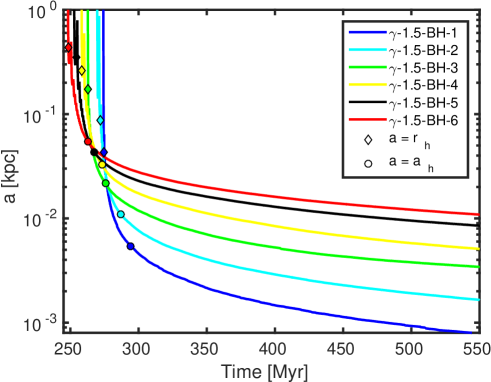
Figure 1: The evolution of the semi-major axes of the six SMBH binaries in the simulations $\gamma$-1.5-BH-1 to $\gamma$-1.5-BH-6. The SMBH binaries harden from the influence radius $r_{\mathrm{h}}$ (open diamonds) to the hard separation $a_{\mathrm{h}}$ (open circles) on a timescale of $\sim 13-20$ Myr, which is between the binary energy transfer timescale $T_{\mathrm{E}}\sim 4.3-6.9$ Myr and the crossing time of the host galaxy, $t_{\mathrm{cross}}\sim 35$ Myr.

The rapid shrinking of the SMBH binaries is accompanied by a sudden decline in the stellar density around the binary, transforming the central stellar cusp of the host galaxy into a flat low-density core (e.g. Milosavljević & Merritt 2001). The evolution of the stellar density profiles in simulations $\gamma$-1.5-BH-0 to $\gamma$-1.5-BH-6 during the core scouring process is presented in Fig. 2. At the time when the SMBHs enter the influence radius $r_{\mathrm{h}}$ of each other, the central stellar cusps of the progenitor galaxies have not yet merged. In order to study the disruption of the stellar cusps, we compute the radial stellar density profiles centered at only one of the SMBHs, with this choice remaining fixed throughout the simulations. Calculating the profile with respect to the center-of-mass of the SMBHs would yield unphysical results for the density of the central region when the stellar cusps are still separated by several kpc and the center-of-mass of the SMBHs lies between the high-density cusps. In the simulation without SMBHs, the center point for the density profile computation is found using the shrinking sphere algorithm taking into account only stars from one of the progenitor galaxies.

The single panel at the top of Fig. 2 shows that in the simulations without SMBHs the stellar density profiles remain practically unchanged after the coalescence of the stellar cusps of the progenitor galaxies. This is consistent with earlier simulation results that showed that the flattening of the density profiles is expected to be mild in collisionless mergers of cuspy progenitors (e.g. Boylan-Kolchin & Ma 2004b). The other panels in Fig. 2 show the evolution of the density profiles in the runs with SMBHs, where the separation of the SMBHs is marked with an open circle for the cases where the separation is larger than the plotting range of $10\ \rm pc$.

The shrinking binaries displace stellar mass from the central region, with the final mass deficit scaling with the mass of the SMBH binary (Merritt, 2006). This is clearly seen especially in the bottom panels with the more massive progenitor SMBHs, for which a flattened central section appears in the density profile when the semi-major axis of the binary shrinks from $a=r_{\mathrm{h}}$ to $a=a_{\mathrm{h}}$. The extent of the flat core and the amount of displaced stellar mass increases systematically as a function of increasing initial SMBH mass. Most of the stellar mass to be displaced from the central region (area between the blue and red lines in Fig. 2) is ejected before $a=a_{\mathrm{h}}$. The density profiles of the run $\gamma$-1.5-BH-0 without SMBHs are presented between $t=280$ Myr and $t=363$ Myr, which coincides approximately to the moments of the SMBH binary becoming bound and subsequently hard in the simulations containing SMBHs.

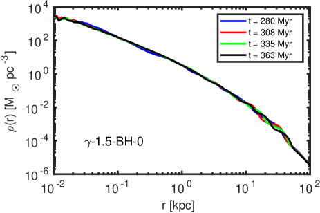
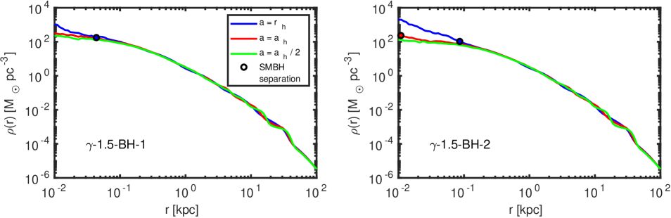
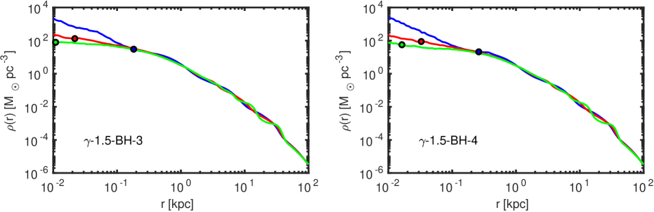
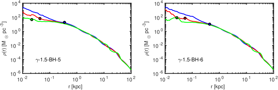
Figure 2: The evolution of the stellar density profiles of the merger remnants during the formation and hardening phases of the SMBH binaries. The profiles are computed with respect to the position of one of the SMBHs, with this choice remaining fixed throughout the simulations. The SMBH separation is indicated with an open circle if above the plotting range of $10$ pc. The mass deficit and the extent of the flat central section increases systematically with increasing initial SMBH mass.

The decline of the central stellar density can also be characterized by the increasing size of the sphere of influence $r_{\mathrm{SOI}}$ of the SMBHs. Here we define $r_{\mathrm{SOI}}$ as the radius enclosing an stellar mass equalling the SMBH mass, $M_{\bullet}$. The evolution of the sphere of influence of an individual SMBH during the core scouring process is presented in Fig. 3. The color coding and symbols describing the different simulations are the same as in Fig. 1. Before the SMBHs form a gravitationally bound binary, the extent of the sphere of influence fluctuates as a response to the changing central stellar density caused by the close passages of the nuclear stellar cusps. After $a=r_{\mathrm{h}}$ (open diamond symbols), the sphere of influence $r_{\mathrm{SOI}}$ rapidly increases as the stellar density around the shrinking SMBH binary strongly declines. This is especially clearly seen in the simulations with more massive SMBHs, which result in larger mass deficits. The phase of rapid evolution of the $r_{\mathrm{SOI}}$ lasts only until the binary becomes hard (open circles), after which the rate of evolution of $r_{\mathrm{SOI}}$ is much slower.

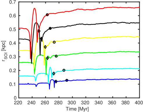
Figure 3: The evolution of the sphere-of-influence of an individual SMBH ($M_{\star}(r_{\mathrm{SOI}})=M_{\bullet}$) during the formation and hardening processes of the SMBH binary. The rapid increase between $a=r_{\mathrm{h}}$ and $a=a_{\mathrm{h}}$ is due to the strong decline in the stellar density as stars are displaced from the central regions by the shrinking binary. This is the time when the stellar core forms. After the binary becomes hard, the sphere-of-influence $r_{\mathrm{SOI}}$ only increases mildly.

The evolution of the two-dimensional surface densities of the merger remnants are presented in Fig. 4 around the time of coalescence of the central stellar cusps. The four rows of Fig. 4 show the stellar surface density in the simulation run $\gamma$-1.5-BH-0 without SMBHs and in the run $\gamma$-1.5-BH-6 with the most massive SMBHs. The spatial extent of the panels is $20$ kpc in the two top rows and $2$ kpc in the two bottom rows. In the run without SMBHs, the central stellar surface density remains high after cusp coalescence, as seen in the top and third panels of Fig. 4, with some stars ejected in shells during the pericenter passages of the cusps. In the simulations that include SMBHs the evolution is qualitatively different, with the central stellar surface density strongly declining due to the shrinking binary (fourth panel in Fig. 4). The stars ejected from the central region end up in the outer parts of the merger remnant and are visible as a diffuse stellar component in the outer parts of the merger remnant as can be seen in the rightmost panel of the second row in Fig. 4.

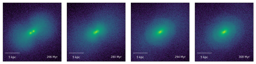
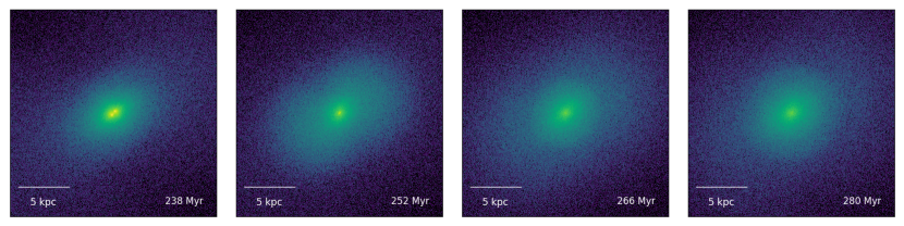
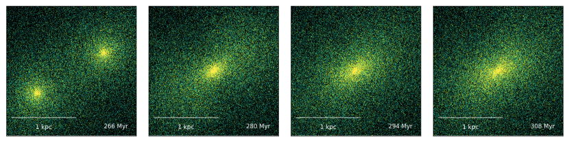
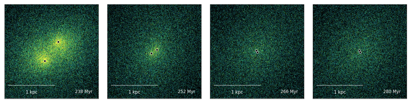
Figure 4: Stellar surface density in the merger simulations at the phase of the coalescence of the central density cusps in $20$ kpc (top two rows) and $2$ kpc frames (bottom two rows) covering 42 Myr of evolution from left to right. The first and third row show the simulation $\gamma$-3/2-BH-0 without SMBHs, while rows two and four present the simulation $\gamma$-3/2-BH-6 with the most massive SMBHs. In the run without SMBHs, the central surface density remains high after the formation of a single nucleus, although some stars are ejected in outward-moving shells. In the run $\gamma$-1.5-BH-6, the central stellar cusps merge somewhat earlier due to the additional dynamical friction caused by the massive SMBHs. The positions of the SMBHs are indicated by circular markers in the panels of the bottom row. During the cusp coalescence, the central surface density is significantly reduced on an timescale of the order of $10$ Myr seen in the bottom panel moving from $t=252\ \rm Myr$ to $t=266\ \rm Myr$. A significant fraction of the stars are ejected from the central region creating an central low-density core (see Fig. 2).

4.2 Destruction of radial orbits

Next, we study the evolution of the stellar velocity dispersion and the velocity anisotropy in the center of the merger remnant. Following T16 we define here the central region as $r<0.19$ kpc. In spherical coordinates, the components of the velocity dispersion can be expressed as $\sigma_{\mathrm{r}}$, $\sigma_{\mathrm{\theta}}$ and $\sigma_{\mathrm{\phi}}$. The two angular dispersions can be combined into the tangential velocity dispersion component $\sigma_{\mathrm{t}}$ defined as

$$\sigma_{\mathrm{t}}=\sqrt{\frac{\sigma_{\mathrm{\theta}}^{2}+\sigma_{\mathrm{\phi}}^{2}}{2}}.$$ (15)

The most commonly used parameter to describe the velocity anisotropy structure of a stellar system is the velocity anisotropy $\beta$ (Binney & Tremaine, 2008), defined as

$$\beta=1-\frac{\sigma_{\mathrm{\theta}}^{2}+\sigma_{\mathrm{\phi}}^{2}}{2\sigma_{\mathrm{r}}^{2}}=1-\frac{\sigma_{\mathrm{t}}^{2}}{\sigma_{\mathrm{r}}^{2}}.$$ (16)

The velocity anisotropy $\beta$ is connected to the orbits of the stellar population. If all the stellar orbits are radial, $\sigma_{\mathrm{t}}=0$ and $\beta=1$. On the other hand, for a stellar population on purely circular orbits $\sigma_{\mathrm{r}}=0$ and $\beta=-\infty$. SMBH binaries can interact strongly with stars that have small pericenter distances, corresponding to low angular momenta. Consequently, SMBH binaries are expected to primarily eject stars on radial orbits and produce a tangentially biased ($\beta<0$) stellar population in the core region. The main aspects of this model have been verified both by numerical simulations (Quinlan & Hernquist, 1997; Milosavljević & Merritt, 2001) and observations (e.g. Thomas et al. 2014).

The evolution of the central radial and tangential velocity dispersions ($\sigma_{\mathrm{r}}$, $\sigma_{\mathrm{t}}$) as well as the velocity anisotropy $\beta$ is presented for the $\gamma=3/2$ simulation sample in Fig. 5. Initially, the radial and tangential velocity dispersions are equal in the vicinity of the SMBHs resulting in $\beta\sim 0$ before the SMBHs form a bound binary. As the binary forms and shrinks from the influence radius $a=r_{\mathrm{h}}$ towards the hard separation $a=a_{\mathrm{h}}$, both the central radial and tangential velocity dispersions increase as more mass is brought into the center of the galaxy. The velocity anisotropy remains still $\beta\sim 0$ in this evolutionary phase.

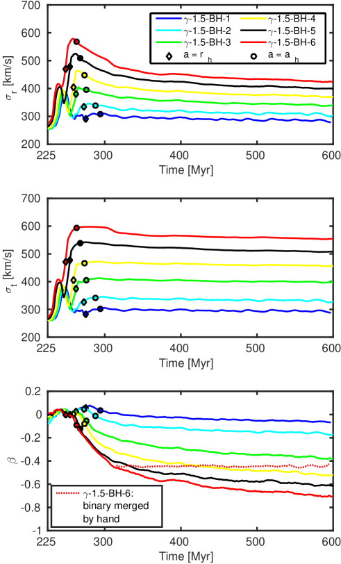
Figure 5: The evolution of the central ($r<0.19$ kpc) radial and tangential components of the stellar velocity dispersion $\sigma_{\mathrm{r}},\sigma_{\mathrm{t}}$ as well as the central velocity anisotropy $\beta$. Both $\sigma_{\mathrm{r}}$ and $\sigma_{\mathrm{t}}$ increase until $a=a_{\mathrm{h}}$. The hard binary ejects stars on radial orbits, causing the radial velocity dispersion to decline while the stars on more circular orbits remain unaffected with $\sigma_{\mathrm{t}}\sim$ constant. The slingshot process results in a tangentially biased velocity structure, with $\beta<0$ in the center of the merger remnants.

The radial velocity dispersion $\sigma_{\mathrm{r}}$ reaches its maximum value almost coincidentally with the SMBH binary becoming hard. After this, the tangential velocity dispersion remains roughly constant while the radial velocity dispersion begins to decline. The decline is stronger for galaxies with higher initial SMBH masses. Consequently, a tangentially biased region with $\beta<0$ is formed in the central region of the galaxy. We performed an additional test simulation to confirm that the SMBH binary scouring indeed causes the decline of the central $\beta$, and that it is not due to numerical effects. The SMBHs of simulation $\gamma$-1.5-BH-6 were merged by hand when $\beta=-0.4$ and the run was restarted. The evolution of the velocity anisotropy in this run is presented with a dotted line in the bottom panel of Fig. 5. The decline of $\beta$ ceases immediately if the SMBHs are merged by hand, confirming that the hard, shrinking SMBH binaries cause the decline of the central velocity anisotropy.

A star which experiences a strong interaction with the SMBH binary is typically ejected with a velocity $v_{\star}$ comparable to the circular orbital velocity of the binary:

$$v_{\star}\sim V_{\mathrm{bin}}=\left(\frac{2GM_{\bullet}}{a}\right)^{1/2},$$ (17)

even though the distribution $f(v_{\star})$ of the ejection velocities is very broad (Valtonen & Karttunen 2006; Merritt 2013). The three-body slingshots become important when the typical ejected star is able to completely escape the host galaxy. A commonly used criterion for escape from a stellar system in N-body studies is $v_{\mathrm{esc}}=2\sqrt{3}\sigma_{\star}$, simplified from $\langle v_{\mathrm{esc}}^{2}\rangle=12\langle\sigma_{\star}^{2}\rangle$, which assumes only the virial theorem and an isotropic velocity dispersion tensor (Spitzer, 1987). For the merger remnants in our simulations, this criterion yields $v_{\mathrm{esc}}\sim 1000$ km/s. In order to study when this occurs in our simulations, we insert the definitions of the influence radius and the hard separation from Eqs. (9) and (13) into the definition of the circular binary velocity Eq. (17). We obtain the typical ejection velocities

$$v_{\star}=\begin{cases}\sqrt{2}\sigma_{\star}\sim 410\hskip 2.84544pt\mathrm{km/s},&a=r_{\mathrm{h}}\\ 4\sigma_{\star}\sim 1160\hskip 2.84544pt\mathrm{km/s},&a=a_{\mathrm{h}}.\\ \end{cases}$$ (18)

At $a=r_{\mathrm{h}}$, the mean stellar ejection velocity is still low and the slingshot mechanism is ineffective. The hard binaries eject stars at typical velocities of $v_{\star}=4\sigma_{\star}>v_{\mathrm{esc}}$, thus the slingshot mechanism is very effective. When the typical ejection velocity equals the escape velocity, $v_{\star}=v_{\mathrm{esc}}$, the semi-major axis of the binary is $a=r_{\mathrm{h}}/6\lesssim a_{\mathrm{h}}$. This is consistent with the radial velocity dispersion $\sigma_{\mathrm{r}}$ reaching its maximum value a few Myr before the binaries become hard, as can be seen in the top panel of Fig. 5. After this point, the binary efficiently destroys radial orbits. As stars on more circular orbits cannot interact strongly with the SMBH binary (pericenter distance $p\gg a$), the tangential velocity dispersions of the merger remnants remain relatively unaffected.

The results in Sections §4.1 and §4.2 indicate that the formation of the low-density core region and the development of the tangentially biased velocity dispersion occur mainly at different times during the evolution of the merger remnant. Most of the stellar mass to be displaced from the core region is removed before the SMBH binary becomes hard at $a=a_{\mathrm{h}}$, whereas most of the central negative velocity anisotropy $\beta$ is built up after this stage. In addition, the timescales of the two processes are very different. The central stellar density declines on a timescale of the order of tens of Myr, which is below the crossing time of the merger remnant. On the contrary, the build-up of the tangentially biased velocity distribution occurs on a timescale of $\sim$ a few hundred Myr, which is several times the crossing time of the merger remnant.

4.3 Binary evolution after core formation

Using KETJU, we include in this study PN corrections up to order 2.5 in the equations of motion of the SMBHs. The PN corrections, and thus the gravitational wave (GW) emission effects are still negligibly small when $a\sim a_{\mathrm{h}}$, excluding the possible but very rare head-on collisions of SMBHs. Eventually, depending on the SMBH binary mass and eccentricity, the PN radiative loss terms in the equations of motion become important. This occurs at the latest when $a\sim a_{\mathrm{GW}}\sim 0.01\times a_{\mathrm{h}}$ (Quinlan, 1996), yielding $a_{\mathrm{GW}}\sim 0.1-1.1$ pc for the binaries in our sample. The binary emits the rest of the orbital angular momentum and energy away as gravitational waves, resulting in a SMBH merger and the formation of a single SMBH.

Averaged over the orbital period, the rates of change of the binary semi-major axis and eccentricity are (Peters & Mathews, 1963)

$$\left\langle\frac{\mathrm{d}a}{\mathrm{d}t}\right\rangle_{\mathrm{GW}}=-\frac{64}{5}\frac{G^{3}M_{1}M_{2}(M_{1}+M_{2})}{c^{5}a^{3}}\frac{1+\frac{73}{24}e^{2}+\frac{37}{96}e^{4}}{(1-e^{2})^{7/2}}$$

$$\left\langle\frac{\mathrm{d}e}{\mathrm{d}t}\right\rangle_{\mathrm{GW}}=-\frac{304}{15}e\frac{G^{3}M_{1}M_{2}(M_{1}+M_{2})}{c^{5}a^{4}}\frac{1+\frac{121}{304}e^{2}}{(1-e^{2})^{5/2}}$$ (19)

assuming that the binary evolution is driven purely by GW emission in the Post-Newtonian order PN2.5. Here $M_{1},M_{2}$ are again the masses of the SMBHs, $a$ is the semi-major axis and $e$ is the eccentricity of the binary. An important property of Peters’ formulas (19) is the extreme dependence of the GW-driven binary evolution on the binary eccentricity. Both $\langle\dot{a}\rangle$ and $\langle\dot{e}\rangle$ diverge in the limit $e\to 1$.

Most of the simulations are run until the SMBHs merge. However, as our main priority lies in studying the core scouring process in the simulated galaxies we do not continue simulation runs with low-eccentricity binaries beyond $t=2$ Gyr. The maximum possible SMBH coalescence timescale in our simulation sample is $t_{\mathrm{coal}}\sim 6$ Gyr, assuming the lowest hardening rate among the simulations (run $\gamma$-1.0-BH-6) and a circular binary with $e=0$ (R17).

4.4 Final surface brightness profiles

The final surface brightness profiles $\mu(r)$ of the merger remnants are presented in Fig. 6. As in T16, we assume a constant stellar mass-to-light ratio of $M_{\star}/L=4.0$ in order to compare the simulated surface density profiles with actual observations. The profiles are azimuthally averaged over $100$ random viewing angles. The outer parts of the simulated merger remnants appear very similar, as expected from the Dehnen profile initial conditions and identical merger orbits. The surface brightness of the simulated galaxies falls below the observed profile of NGC 1600 at $r\sim 30$ kpc.

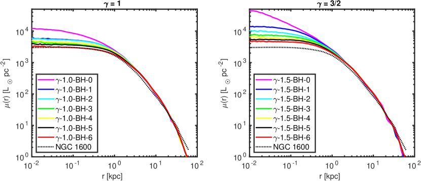
Figure 6: The final surface brightness profiles (solid lines) of the merger simulations with $\gamma=1$ (left panel) and $\gamma=3/2$ (right panel). We assume a constant stellar mass-to-light ratio of $M/L_{\odot}=4.0$. In both cases the central surface brightness decreases and the core size increases with increasing initial SMBH mass. For comparison, we show the observed profile of NGC 1600 (T16) as the black dotted line. We find that the agreement is best for simulations for which the final SMBH mass is similar to the SMBH mass inferred for NGC 1600.

Studying the central parts of the simulated merger remnants, the surface brightness profiles in the runs that include SMBHs turn almost flat at $0.1$ kpc $\lesssim r_{\mathrm{b}}\lesssim 1$ kpc. The profiles of the merger remnants without SMBHs remain cuspy until the very center. We also immediately see that the central surface brightness is lower for the $\gamma=1$ initial conditions compared to the $\gamma=3/2$ runs with the same SMBH mass. In addition, the central surface brightness decreases and the core size (extent of the flat section) increases as the initial SMBH mass increases in both progenitor galaxy samples. This is consistent with the mass deficit arguments in the literature, which states that the mass deficit is proportional to the total mass of the SMBH binary (e.g. Merritt 2006).

The agreement with the observations is best in the simulations with the final SMBH mass similar to $M_{\bullet}=1.7\times 10^{10}M_{\odot}$ inferred for NGC 1600. However, there is some ambiguity here because of the assumed stellar mass-to-light ratio $M_{\star}/L=4.0$ (van Dokkum et al., 2017). With larger values for the mass-to-light ratio $M_{\star}/L>4.0$, simulated galaxies with lower $M_{\bullet}$ or steeper initial stellar density profiles could also match the central surface brightness of NGC 1600. However, with $M_{\star}/L>4.0$, the outer parts of the simulated galaxies would end up too dim compared to the observations. As NGC 1600 is in a group environment, the galaxy has most likely experienced several minor mergers that have puffed up and brightened the outer parts of the galaxy, as opposed to our isolated merger models (e.g. Hilz et al. 2012, 2013). Based solely on surface brightness data, we cannot exactly state which one of the simulated galaxies most closely resembles the observed NGC 1600, and additional velocity data is required for this.

4.5 Final velocity anisotropy profiles

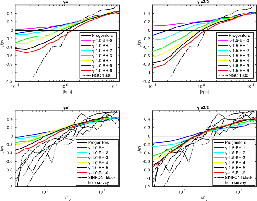
Figure 7: The velocity anisotropy profiles $\beta(r)$ (thick solid lines) in the merger simulations with $\gamma=1$ (left column) and $\gamma=3/2$ (right column). The isotropic progenitor galaxies are presented as thin horizontal solid lines with $\beta(r)=0$. The dynamical model for NGC 1600 (T16) is shown as the dotted line in the two top panels. In the central region ($r<1$ kpc), $\beta$ becomes increasingly more negative with increasing initial SMBH mass, indicating an increasingly more tangentially biased stellar population. The mergers with more cuspy initial stellar density profiles develop a steeper $\beta$ profile. The simulations with the largest initial SMBH masses agree best with the dynamical model of NGC 1600. We see a trend in which the steeper initial density cusp runs produce better agreement with the inferred dynamical model for NGC 1600. The two bottom panels present the $\beta$ profiles of the merger simulations with the radial coordinate scaled by the break radius $r_{\mathrm{b}}$ of the surface brightness profiles. The models of the observed galaxies from the SINFONI black hole survey (Thomas et al., 2014; Saglia et al., 2016) are plotted as dotted lines. Again, increasing the initial SMBH mass and the steepness of the slope for initial stellar density profile produces merger remnants in better agreement with the dynamical models of the observed galaxies.

The final velocity anisotropy profiles $\beta(r)$ of the simulated galaxies are presented in Fig. 7. The velocity anisotropy is computed in radial bins, with the bin width $\Delta r=0.19$ kpc motivated by the spatial resolution of the spectral data in T16. For comparison, the isotropic $\beta$ profiles of the progenitor galaxies are also shown as horizontal lines. The top panels compare the $\beta(r)$ of the simulated galaxies to the dynamical model of NGC 1600 (T16). Without the inclusion of SMBHs, the velocity structure of the mergers remnants of both the $\gamma=1$ and $\gamma=3/2$ samples is close to isotropic in the center of the galaxy.

In the outer parts, the stellar population is dominated by radial orbits ($\beta\sim 0.40$-$0.45$ at $r=10$ kpc) which is typical for collisionless mergers (Röttgers et al., 2014). The outer parts of the merger remnants with SMBHs are almost identical to the remnants without SMBHs. The dynamical model of NGC 1600 is more radially biased at radii beyond $r\gtrsim 3$ kpc, with ($\beta\sim 0.5$-$0.6$ at $r=10$ kpc). The smaller amount of stellar material on radial orbits in the outer parts can be explained by the lack of minor merges in our isolated major merger simulation, as already discussed in the previous section. However, it should be noted that the velocity structure of the stellar population in the outer parts of the simulated merger remnants show still qualitatively similar trends to the dynamical model of NGC 1600, at least when compared to the isotropic progenitor galaxies.

The central parts ($r\lesssim 1$ kpc) of the simulated merger remnants have a tangentially biased stellar population ($\beta<0$). There is a clear trend of increasingly more negative $\beta$ with the increasing initial SMBH mass. In addition, more cuspy initial stellar profiles produce steeper $\beta$ profiles in the core region, consistent with the results of Bortolas et al. (2018). The dynamical model of NGC 1600 has an even steeper $\beta$ profile near the center when compared to the simulations. This suggests that the initial stellar density profiles for the progenitors of NGC 1600 were even steeper than $\gamma=3/2$. We note that the final central values of $\beta$ depend on the chosen isotropic initial conditions. A second generation of mergers would already have $\beta<0$ initially, leading to an increasingly tangential central stellar population. In addition, other physical processes such as the adiabatic growth of the single central SMBH may decrease $\beta$ as well (e.g. Goodman & Binney 1984; Thomas et al. 2014).

The bottom panels of Fig. 7 present the same simulated anisotropy profiles as in the top panels, but the radial coordinate is now scaled with the break radius $r_{\mathrm{b}}$ of the surface brightness profile. The determination of the break radius $r_{\mathrm{b}}$ is discussed in §5.2. The $\beta$ profiles of dynamical models of six observed core galaxies from the SINFONI black hole survey (Thomas et al., 2014; Saglia et al., 2016) are presented for comparison. Observed massive elliptical galaxies with cores have remarkably similar velocity anisotropy profiles when scaled with the core radius $r_{\mathrm{b}}$. In the outer parts ($r/r_{\mathrm{b}}>2$-$3$), the $\beta$ profiles of the simulated merger remnants and the galaxies from the SINFONI black hole survey now agree very well. At even larger radii $(r/r_{\mathrm{b}}>10)$ the simulated profiles agree with the lower end of the distribution of observed profiles. In the core region ($r/r_{\mathrm{b}}<1$), the profiles of the simulated merger remnants coincide with the upper end of the observed anisotropies in the SINFONI black hole survey. Increasing the initial SMBH mass and selecting a steeper stellar density profile slope results in merger remnants in better agreement with the dynamical models of the galaxies from the SINFONI black hole survey. Again, we note that the assumption of a single generation of galaxy mergers with isotropic initial conditions affects the results discussed here. An additional generation of mergers would start with $\beta<0$ in the center and $\beta>0$ in the outer parts of the galaxies, potentially leading to a better agreement with the observed galaxies.

In summary, the results of our surface brightness profile and velocity anisotropy analysis support the SMBH mass $M_{\bullet}=1.7\times 10^{10}M_{\odot}$ obtained by the dynamical modeling of T16 and suggest steep initial stellar profiles with $\gamma\geq 3/2$ for the progenitor galaxies of NGC 1600.

4.6 2D kinematics maps

We show in Figures 8 and 9 the two dimensional kinematic maps for the $\gamma=1$ and $\gamma=3/2$ simulation samples, respectively. The maps are constructed similarly to what an observer would see if the merger remnants were observed with an Integral Field Unit spectrograph (see Naab et al. 2014). Following the same procedures used in analyzing observational data, each panel is divided into ”spaxels” with the same signal-to-noise, using the Voronoi tessellation algorithm (Cappellari & Copin, 2003). In our case the signal-to-noise is represented by the number of particles in each bin. For each row in the two figures, the four panels show from left to right, the average line-of-sight velocity $V_{\mathrm{avg}}$, the line-of-sight velocity dispersion $\sigma$, and the $h_{3}$ and $h_{4}$ parameters, which represent the skewness and kurtosis of the line-of-sight (LOS) velocity distribution (van der Marel & Franx, 1993; Gerhard, 1993). These parameters are calculated by fitting the histogram of LOS velocities in every spaxel with the following modified Gaussian function:

$$f(v)=I_{0}\,e^{-y^{2}/2}(1+h_{3}\,H_{3}(y)+h_{4}\,H_{4}(y))$$ (20)

where $y=(v-V_{\rm avg})/\sigma$ and $I_{0}$ is a normalization constant. Here $H_{3}$ and $H_{4}$ are the Hermite polynomials of third and fourth order:

$$H_{3}(y)=(2\,\sqrt{2}\,y^{3}-3\,\sqrt{2}\,y)/\sqrt{6}$$ (21)

$$H_{4}(y)=(4\,y^{4}-12\,y^{2}+3)/\sqrt{24},$$ (22)

Before performing this analysis, the galaxies are oriented using the reduced inertia tensor so that their major axis is on the x axis of the figure, and the LOS velocities are centered so that the spaxels within the central kpc in projection have zero average velocity. We also plot luminosity contours with a spacing of one magnitude on top of each velocity map.

In the merger remnants without SMBHs, the central regions show a positive $h_{4}$ peak. This is typical for nearly isotropic galaxies with SMBHs and not too steep central stellar cusps (Baes et al., 2005). However, in simulations including SMBHs, we find systematically more negative $h_{4}$ values as a function of increasing SMBH mass (see bottom rows of Figs. 8 and 9). The size of the negative $h_{4}$ region also grows with increasing SMBH mass and increasing size of the sphere of influence. The lower values of $h_{4}$ likely result from the missing weakly bound stars on low-angular-momentum orbits.

In the velocity maps a central kpc-scale, decoupled rotating region becomes increasingly more visible as the SMBH mass increases. There are even indications of more complex kinematic subsystems in the merger remnants $\gamma$-1.5-BH-4 to $\gamma$-1.5-BH-6. As can be seen in the bottom panels of Fig. 9 a large ($\sim 5$ kpc) region counter-rotating to the central rotating region becomes apparent in the simulations containing the more massive SMBHs. The $h_{3}$ map shows an anti-correlation to the LOS velocity map, which is commonly observed in rotating systems (e.g. Bender et al. 1994; Krajnović et al. 2011; Veale et al. 2017). Finally, the stellar velocity dispersion increases also because of the increased mass in the central region for larger SMBH masses.

In conclusion, Fig. 8 & Fig. 9 clearly demonstrate that the effects of black hole scouring are indeed observable in the kinematic maps of quiescent merger remnants.

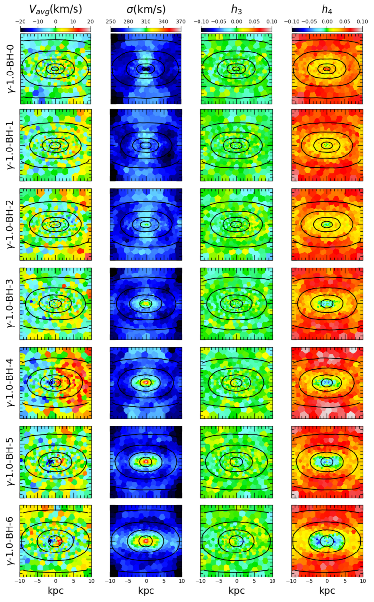
Figure 8: Two-dimensional stellar kinematic maps of the simulations with $\gamma=1$, the SMBH mass is increasing from top to bottom. Shown are the line-of-sight velocity $V_{\mathrm{avg}}$, the stellar velocity dispersion $\sigma$, $h_{3}$ and $h_{4}$ from left to right. Luminosity isophote contours are overlaid with a spacing of one magnitude. The systems with higher SMBH masses are developing a rotating, high-dispersion decoupled core with clearly anti-correlated $h_{3}$ and $V_{\mathrm{avg}}$, as well as a negative $h_{4}$.

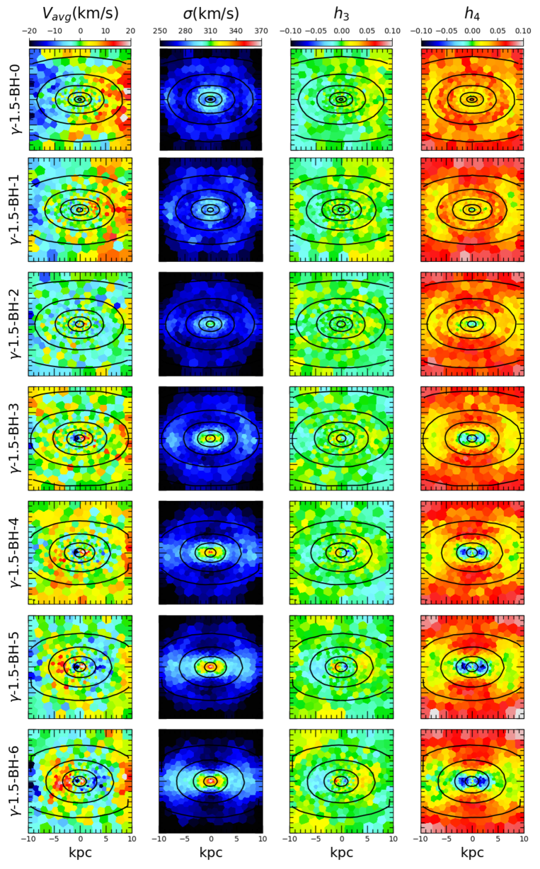
Figure 9: The same figure as Fig. 8 but for simulations with $\gamma$=3/2. For this simulation sample the rotating central feature becomes also more prominent for higher initial SMBH masses. There are even indications in the line-of-sight velocity $V_{\mathrm{avg}}$ and $h_{3}$ maps for more complex kinematic subsystems in the merger remnants $\gamma$-1.5-BH-4 to $\gamma$-1.5-BH-6.

5 Scaling relations

5.1 Observed and simulated galaxy samples

In T16 tight scaling relations are presented between the observed galaxy core sizes (or break radii) $r_{\mathrm{b}}$, the SMBH masses $M_{\bullet}$ and the spheres of influence of the SMBHs $r_{\mathrm{SOI}}$. We perform a similar analysis for our simulated merger remnants. In addition, we use a simple core scouring model to interpret the results of our merger simulations.

It should be noted that while our merger simulation sample consists of single-mass remnants with $M_{\star}=M_{\star}^{\mathrm{NGC1600}}=8.3\times 10^{11}M_{\odot}$, the scaling relations of T16 are obtained from a broader core galaxy sample. The core galaxies in the T16 sample have total stellar masses in the range from $M_{\star}=5.0\times 10^{10}M_{\odot}$ to $2.0\times 10^{12}M_{\odot}$, with a mean stellar mass of $\langle M_{\star}\rangle=5.8\times 10^{11}M_{\odot}$ (Rusli et al., 2013a, b; Saglia et al., 2016). The mean effective radius is approximately $\langle R_{\mathrm{e}}\rangle=8.5$ kpc. The velocity dispersions of the observed sample are in the range $168<\sigma_{\star}<380$ km/s with a mean of $\langle\sigma_{\star}\rangle=289$ km/s. This agrees reasonably well with the velocity dispersions of our simulated merger remnants, for which $\sigma_{\star}\sim 290$ km/s. In the T16 sample the SMBH masses span from $4.2\times 10^{8}M_{\odot}$ to $2.1\times 10^{10}M_{\odot}$ with an average of $\langle M_{\bullet}\rangle=3.5\times 10^{9}M_{\odot}$. This is in a similar range to the final SMBH masses in our merger simulations: $1.7\times 10^{9}M_{\odot}<M_{\bullet}<1.7\times 10^{10}M_{\odot}$.

Even though the stellar mass and the velocity dispersion in our simulated galaxies lie close to the mean values of the T16 observational sample, we stress that some care should be taken in the interpretation of our simulated core scaling relations. The interpretation boils down to the central question of how local the core scouring process is. Thus, the question is whether the properties of the host galaxy beyond $r_{\mathrm{SOI}}$ strongly affect the core formation process or whether the core formation process is mainly dictated by the mass of the SMBH. The results in §4.1 support the latter scenario, as the central core forms rapidly compared to the crossing time of the merger remnant, when the SMBH binary shrinks from $a=r_{\mathrm{h}}$ to $a=a_{\mathrm{h}}$. However, on the other hand if the large-scale properties of the host galaxies strongly affect the core scouring process, we should not be able to reproduce the observed scaling relations using only single-mass progenitor galaxy models.

5.2 Determining the core size

There are a number of widely-used methods to determine the size of the cored region in the surface brightness profile $\mu(r)$. One popular model is the six-parameter Core-Sérsic profile (Graham et al. 2003; Trujillo et al. 2004), which is defined as

$$\mu(r)=\mu^{\prime}\left[1+\left(\frac{r_{\mathrm{b}}}{r}\right)^{\alpha}\right]^{\gamma/\alpha}e^{-b\left[\left(r^{\alpha}+r_{\mathrm{b}}^{\alpha}\right)/R_{\mathrm{e}}^{\alpha}\right]^{1/(\alpha n)}}.$$ (23)

In the outer parts, the profile follows the ordinary three-parameter Sérsic profile (Sérsic, 1963; Caon et al., 1993) defined by the Sérsic index $n$, the effective radius $R_{\mathrm{e}}$ and the overall normalization $\mu^{\prime}$. Towards the central regions, the core-Sérsic profile breaks away from the Sérsic profile at the break radius (i.e. the core size) $r_{\mathrm{b}}$ to allow for a shallow central power-law with a slope $\gamma$. The parameter $\alpha$ determines how sudden this break is. Finally, the constant $b$ is determined by requiring that the effective radius $R_{\mathrm{e}}$ encloses half of the total light of the core-Sérsic profile.

We perform the profile fitting using the CMPFIT Library. The radial fitting range for all the surface brightness profiles shown in Fig. 6 is $0.01$ kpc $<r<62$ kpc in this Section, similar to T16. For all of these fits the core-Sérsic index is fixed to $n=4$. The reason for this procedure is to avoid any possible degeneracy between the Sérsic index and the break radii in the fitting procedure (Dullo & Graham, 2012), and to compare the results from subsamples $\gamma=1$ and $\gamma=3/2$ with each other in a more straightforward and robust manner. If we allow the Sérsic index to freely vary, we typically get $n\leq 3$ for the $\gamma=1$ simulation sample, which is on the low side for massive early-type galaxies, see e.g. the Appendix A of Naab & Trujillo (2006) for details. The initial surface brightness profiles of the $\gamma=3/2$ sample are best fit with the Sérsic indices close to $n=4$ (Dehnen, 1993), making these initial conditions more in tune what would be expected for massive early-type galaxies.

Another option is to fit the so-called Nuker profile (Lauer et al., 1995) to the surface brightness profile, defined as

$$\mu(r)=\mu_{\mathrm{b}}2^{(\beta-\gamma)/\alpha}\left(\frac{r}{r_{\mathrm{b}}}\right)^{-\gamma}\left[1+\left(\frac{r}{r_{\mathrm{b}}}\right)^{\alpha}\right]^{(\gamma-\beta)/\alpha},$$ (24)

where $r_{\mathrm{b}}$ is the break radius, $\gamma$ is the logarithmic slope of the profile inside and $\beta$ is the logarithmic slope outside the break radius. The parameter $\alpha$ again measures the sharpness of the transition from the inner to the outer power-law at the break radius, $r=r_{\mathrm{b}}$ . The Nuker profile was originally used to fit the Hubble Space Telescope observations of early-type galaxies within the central 10 arcseconds. At the distance of NGC 1600 this corresponds to $\sim 3.1$ kpc. Later, the Nuker profile has also been used to fit the surface brightness profiles in the entire radial range of observed galaxies. However, it is well known that the parameters of the Nuker profile depend on the radial fitting range (Graham et al., 2003).

We performed the Nuker profile fits first in the same radial range as for the core-Sérsic fits ($0.01$ kpc $<r<62$ kpc). In this case the best-fit Nuker profiles for all the galaxies in our simulated galaxy sample have $\alpha<1$. In general, when $\alpha\lesssim 1$, the presence of two power-laws may not emerge and instead one continuous curving arc describes the profile (Graham et al., 2003). Consequently, the break between the inner and outer profiles is not well defined. We tested whether stacking of the surface brightness profiles from different viewing angles or using elliptical rather than circular bins in Fig. 6 would affect the results, but we still found $\alpha<1$ for all the Nuker fits. However, we found that when the outer edge of the radial fitting range is chosen to be below $2\times R_{\mathrm{e}}$, the sharpness parameter $\alpha$ becomes larger than unity. The core size $r_{\mathrm{b}}$ thus also depends on the radial fitting range, which is consistent with findings in the literature (Graham et al. 2003). Next, we performed the Nuker fits only in the central parts of the surface brightness profile in the range $0.01$ kpc $<r<3.1$ kpc. Now we found $\alpha>1$ for all the simulated galaxies expect $\gamma$-1.5-BH-2. The core sizes obtained from the core-Sérsic and the central Nuker fits are compared in Fig. 10. We find that the Nuker break radii are systematically larger than the core-Sérsic core radii, especially in the simulation set with $\gamma=1$.

Finally, a simple non-parametric method can also be used to estimate the core size by studying the logarithmic slope of the surface brightness profile. The ”cusp radius” $r_{\gamma}$ can then be defined as

$$\left[\frac{\mathrm{d}\log{\mu(r)}}{\mathrm{d}\log{r}}\right]_{r=r_{\gamma}}=-\frac{1}{2},$$ (25)

i.e. as the point where the logarithmic slope of the surface brightness profile, $\mu(r)$, equals $-1/2$ (Carollo et al. 1997; Lauer et al. 2007). We find that the cusp radii $r_{\gamma}$ of our simulated galaxies are consistent with the core radii derived from the core-Sérsic fits (see Fig. 10).

In this study, we use the core-Sérsic break radius $r_{\mathrm{b}}$ to measure the sizes of the cores of our simulated galaxies. This selection makes the comparison with T16 straightforward. The Nuker fits are not used in the following sections because of their dependence on the radial fitting range and the $\alpha<1.0$ problem encountered while fitting our simulated surface brightness profiles. The cusp radii $r_{\gamma}$ could also be used in the following analysis, as the core sizes using the method are consistent with the results obtained using the core-Sérsic fit, which was also found by T16.

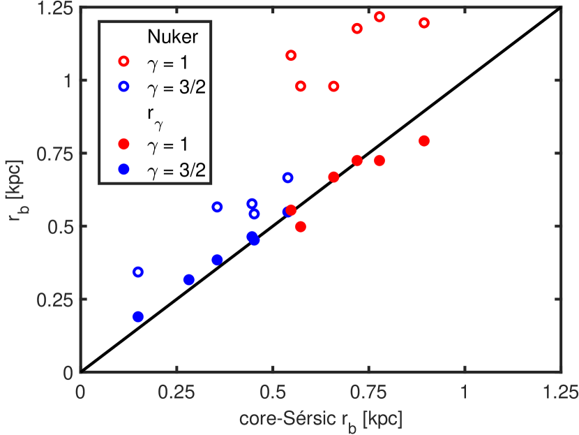
Figure 10: A comparison of different core size determination methods for our simulated surface brightness profiles. The core radii obtained using the non-parametric $r_{\gamma}$ method agree well with the core-Sérsic break radii $r_{\mathrm{b}}$, whereas the Nuker break radii are systematically larger. Note that the Nuker core sizes strongly depend on the selected radial fitting range, as discussed in the text. Here the fitting range is $0.01$ kpc $<r<3.1$ kpc for the Nuker fit.

5.3 Simple scouring model

We use a simple core scouring model to interpret the results of our simulations. Starting from the stellar density profile $\rho(r)$ in our initial conditions we first remove a mass deficit equaling the mass of the SMBH, i.e. $M_{\mathrm{def}}=M_{\bullet}$. This choice is motivated both by observations and N-body simulations (see e.g. Merritt 2013). The stellar mass is removed from the density profile in such a way that the central part of the scoured density profile $\rho_{\mathrm{s}}(r)$ becomes flat up to the deficit radius $r_{\mathrm{def}}$:

$$\rho_{\mathrm{s}}(r)=\begin{cases}\rho(r),&r\geq r_{\mathrm{def}}\\ \rho(r_{\mathrm{def}}),&r<r_{\mathrm{def}}.\end{cases}$$ (26)

The mass deficit is therefore

$$M_{\mathrm{def}}=4\pi\int_{0}^{r_{\mathrm{def}}}\left[\rho(r)-\rho(r_{\mathrm{def}})\right]r^{2}dr,$$ (27)

from which the mass deficit radius can be solved numerically. The deficit radius $r_{\mathrm{def}}$ is sometimes also referred to as the core radius (e.g. Volonteri et al. 2003), but we reserve this label for the break radius $r_{\mathrm{b}}$ obtained from the core-Sérsic fit (Eq. 23) of the surface brightness profile.

Next, we measure the extent of the sphere of influence of the SMBH from the flattened density profile $\rho_{\mathrm{s}}(r)$. Instead of using the definition of $r_{\mathrm{h}}$ from Eq. (9), we follow here T16 and define the sphere of influence $r_{\mathrm{SOI}}$ using the enclosed mass as

$$M_{\star}(r_{\mathrm{SOI}})=4\pi\int_{0}^{r_{\mathrm{SOI}}}\rho_{\mathrm{s}}(r)r^{2}dr=M_{\bullet}.$$ (28)

The sphere of influence $r_{\mathrm{SOI}}$ is then again most conveniently solved numerically.

The two-dimensional surface brightness profile $\mu(r)$ is obtained by projecting the analytically scoured density profile. Labeling the constant stellar mass-to-light ratio as $M_{\star}/L=\Upsilon_{\star}$, the surface brightness profile can be computed from

$$\mu(r)=\Upsilon_{\star}\Sigma(r)=2\Upsilon_{\star}\int_{r}^{\infty}\frac{\rho_{\mathrm{s}}(r^{\prime})r^{\prime}}{\sqrt{r^{\prime 2}-r^{2}}}dr^{\prime}.$$ (29)

Finally, the break radii $r_{\mathrm{b}}$ of the generated surface brightness profiles are obtained from the core-Sérsic fitting procedure as described in the previous section.

5.4 Results

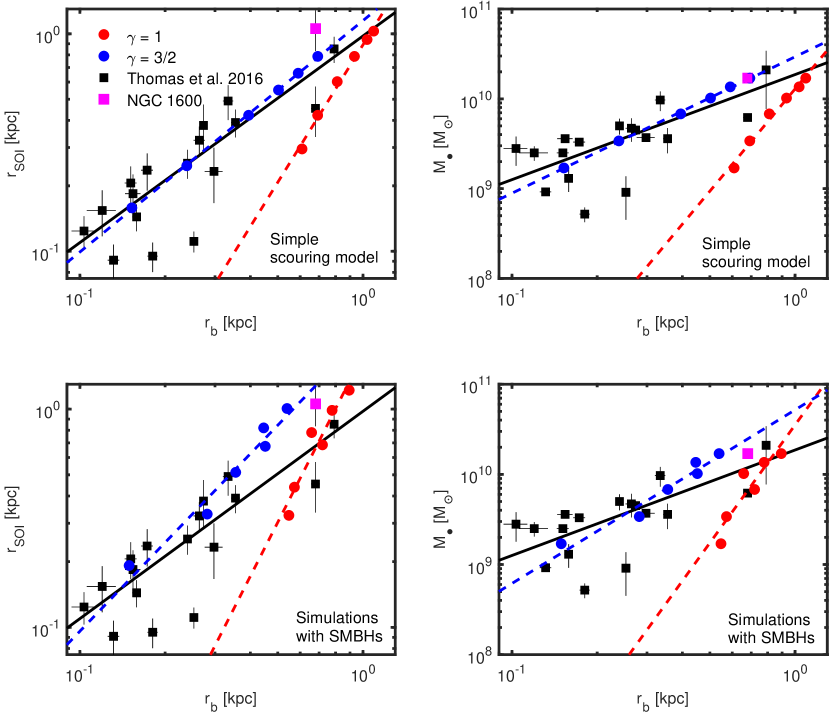
Figure 11: Core scaling relations $(r_{\mathrm{b}}$ vs. $r_{\mathrm{SOI}})$ in the left column and $(r_{\mathrm{b}}$ vs. $M_{\bullet})$ in the right column. The top panels present the relations obtained using the simple scouring model described in §5.3. The bottom panels show the relations obtained from the merger simulations. The observed galaxies by T16 are marked as black squares with 1-sigma uncertainties. The fitted scaling relation is shown as the black solid line. NGC 1600 is highlighted as the large magenta square in each plot. The relations from the simple scouring model agree qualitatively very well with the merger simulation relations. For steeper initial stellar density profiles $(\gamma=1.5)$ the agreement between both the analytic and simulated slopes is better with the observations.

$\log_{10}(r_{\mathrm{SOI}}/\mathrm{kpc})=a_{1}+b_{1}\log_{10}(r_{\mathrm{b}}/\mathrm{kpc})$
	$a_{1}$	$b_{1}$
Thomas et al. (2016)	$-0.01\pm 0.29$	$0.95\pm 0.08$
Simple model $\gamma=1$	$-0.05\pm 0.01$	$2.10\pm 0.08$
Simulation $\gamma=1$	$0.25\pm 0.03$	$2.55\pm 0.22$
Simple model $\gamma=3/2$	$0.06\pm 0.01$	$1.06\pm 0.01$
Simulation $\gamma=3/2$	$0.33\pm 0.07$	$1.35\pm 0.17$

$\log_{10}(M_{\bullet}/M_{\odot})=a_{2}+b_{2}\log_{10}(r_{\mathrm{b}}/\mathrm{kpc})$
	$a_{2}$	$b_{2}$
Thomas et al. (2016)	$10.27\pm 0.51$	$1.17\pm 0.14$
Simple model $\gamma=1$	$10.11\pm 0.01$	$3.78\pm 0.19$
Simulation $\gamma=1$	$10.55\pm 0.09$	$4.35\pm 0.58$
Simple model $\gamma=3/2$	$10.47\pm 0.01$	$1.52\pm 0.01$
Simulation $\gamma=3/2$	$10.72\pm 0.11$	$1.93\pm 0.28$

Table 3: The parameter values of the core scaling relations ($r_{\mathrm{b}}$ vs. $r_{\mathrm{SOI}}$) and ($r_{\mathrm{b}}$ vs. $M_{\bullet}$) presented in Fig. 11. The constant term $a$ from both the simple scouring model and the merger simulations are within the uncertainty of the observed relation of T16. We also see a trend for both the analytic and simulated slopes $b$ towards the observed slope values of $b\sim 1$ for steeper initial stellar density profiles, with the steeper $\gamma=1.5$ profiles providing clearly a better match with the observations.

We derive the break radii $r_{\mathrm{b}}$ of the surface brightness profiles of our simulated merger remnants using the fitting procedure described in §5.2. The residuals of the fits are of the same order as the residuals of the observed core-Sérsic of NGC 1600 presented in T16, that is below $\Delta\mu<0.1$ mag. The extents of the spheres of influence $r_{\mathrm{SOI}}$ are obtained directly from the simulation data using the enclosed stellar mass definition (see Eq. 28). These parameter values comprise the core data points ($r_{\mathrm{b}},r_{\mathrm{SOI}}$), ($r_{\mathrm{b}},M_{\bullet}$) of the merger simulations.

We produce another set of ($r_{\mathrm{b}},r_{\mathrm{SOI}}$), ($r_{\mathrm{b}},M_{\bullet}$) data points using our simple scouring model and the 12 initial conditions of the merger simulations containing central SMBHs. The actual scaling relations for both the simulation samples and the analytical scouring models are obtained by fitting the free parameters $a_{1},b_{1},a_{2},b_{2}$ in the fitting functions

$$\log_{10}(r_{\mathrm{SOI}}/\mathrm{kpc})=a_{1}+b_{1}\log_{10}(r_{\mathrm{b}}/\mathrm{kpc})$$ (30)

$$\log_{10}(M_{\bullet}/M_{\odot})=a_{2}+b_{2}\log_{10}(r_{\mathrm{b}}/\mathrm{kpc}).$$

The values of the best fit parameters are listed in Table 3, where the error estimates have been computed using a simple bootstrap method. The results from both the merger runs and the simple scouring model are presented in Fig. 11. The simulation data points and the simple scouring model points are plotted as red ($\gamma=1$) and blue ($\gamma=1.5$) filled circles, respectively. The scaling relations for both of the $\gamma=1$ and $\gamma=3/2$ subsamples are plotted as dotted lines of the corresponding color. The observed galaxy sample of T16 is shown as black squares, with the solid lines representing the observed scaling relations $\log_{10}(r_{\mathrm{SOI}}/\mathrm{kpc})=(-0.01\pm 0.29)+(0.95\pm 0.08)\log_{10}(r_{\mathrm{b}}/\mathrm{kpc})$ and $\log_{10}(M_{\bullet}/M_{\odot})=(10.27\pm 0.51)+(1.17\pm 0.14)\log_{10}(r_{\mathrm{b}}/\mathrm{kpc})$.

Studying Fig. 11, we see that our simple scouring model produces qualitatively similar results to the major merger simulations. We also see a trend towards the observed relations with increasing initial stellar density profile slope $\gamma$, as the scaling relations flatten for steeper initial stellar profiles. This fact points towards very cuspy initial stellar density profiles of the progenitor galaxies, with $\gamma$ in excess of $3/2$, in the framework of a single generation of galaxy mergers. Mergers of galaxies with relatively flat Hernquist-like stellar bulges ($\gamma=1$) result in too steep core scaling relations. Finally, we also note that our core scaling relations are consistent with the results of Lauer et al. (2007), who obtained the $M_{\bullet}$-$r_{\gamma}$ -relation from a sample of 11 observed core galaxies using directly determined SMBH masses.

5.5 Central homology of power-law ellipticals

The surprisingly good agreement between the scaling relations derived from our cuspier $(\gamma=1.5)$ initial conditions and the observed relations requires an explanation. All the progenitor galaxies in our merger simulation sample had identical stellar density profiles and in practise identical velocity profiles outside of $r>r_{\mathrm{SOI}}$, while the observed T16 galaxy sample had a broad range of stellar mass and velocity dispersions, as described in §5.1.

Both observations and simulations have shown that the total density profiles of power-law galaxies are well represented with simple density profiles $\rho\propto r^{-\gamma}$ over a wide range in radius, with $\gamma\sim 2.0$-$2.2$ (e.g. Cappellari et al. 2015; Remus et al. 2013, 2017 and references therein). At $r\ll r_{1/2}$, the stellar component dominates the total density profile, so the stellar density profile has a central slope $\gamma\sim 2$. In order to estimate the mean central stellar densities $\rho$ of the power-law galaxies, we model the stellar component using the Dehnen profile as in §3.1 with $\gamma=2$. We sample a large number of progenitor galaxy models with parameters $M_{\bullet}$, $M_{\star}$ and $r_{1/2}$ and their uncertainties from T16 and Saglia et al. (2016). Next, we compute the mean central $(r<1\ \rm pc)$ stellar densities for these idealized galaxy models. Although the stellar mass increases by a factor of $40$ from $\min(M_{\star}^{\mathrm{T16}})$ to $\max(M_{\star}^{\mathrm{T16}})$, the central stellar density increases simultaneously only by a factor of $6.2\pm 3.8$ from the most diffuse galaxy to the galaxy with the highest central density. Thus, the central stellar density increases slowly compared to the total stellar mass. The population of power-law galaxies is very homogeneous in their central stellar density properties. At the same time, the mass of the SMBH, $M_{\bullet}$ in the T16 sample increases much more significantly, by a factor of $\sim 50$.

We argue that this homology of the central properties of the power-law ellipticals is responsible for the good correspondence between the core scaling relations from our single-$M_{\star}$ merger simulation sample and the scaling relations of the observed core galaxy population. Our results support the scenario in which the progenitors of the most massive core ellipticals are cuspy power-law galaxies ($\gamma>3/2$) with central SMBHs. The central properties of the stellar population are fairly homogeneous over a large range in $M_{\star}$, while the SMBH masses steadily increase as $M_{\star}$ grows. Thus, the SMBH mass $M_{\bullet}$ stands out as the main parameter in the core scouring process and is also responsible for determining the core scaling relations.

6 Conclusions

We have performed a series of galaxy merger simulations that include supermassive black holes using the regularized tree code KETJU. The study presented in this paper mainly concentrated on two parameters: the initial SMBH mass $M_{\bullet}$ and the central slope of the initial stellar density profile, $\gamma$. The properties of the progenitor galaxies were selected in such a way that the simulated merger remnant would be a close analogue to the observed core elliptical galaxy NGC 1600, which was extensively studied in T16.

From the simulated merger remnants we find a systematic decrease in the central surface brightness and increasingly more tangentially biased central velocity anisotropies (decreasing $\beta$) as a function of increasing SMBH mass in the initial conditions. Similar dynamical trends can also be seen in the mock stellar 2D kinematic maps. In addition, the kinematic maps also reveal decoupled, kpc-scale rotating regions which become more apparent for increasing SMBH masses. Finally, there are indications of even more complex kinematic subsystems in the $\gamma=3/2$ merger remnants with the most massive initial SMBH masses. Overall, we find the best match between our simulated merger remnants and the observed NGC 1600 galaxy for the simulation run with the SMBH masses inferred for NGC 1600 by the dynamical modeling of T16. For a single generation of mergers, especially the velocity anisotropy profiles favor cuspy initial stellar profiles for the progenitor galaxies with very steep profiles in excess of $\gamma\gtrsim 3/2$.

We also study the time evolution of the core scouring process in detail. Our simulated galaxy mergers with larger initial SMBH masses result is merger remnants with systematically larger cores, in good agreement with earlier findings (e.g. Merritt 2006). Defining the core formation as the moment when the central density profile flattens, the formation process is very rapid and occurs when the semi-major axis of SMBH binary shrinks from the influence radius to the hard radius, i.e. from $a=r_{\mathrm{h}}$ to $a=a_{\mathrm{h}}$. When the SMBH binaries become hard, the destruction of the radial orbits commences and the core regions of the merger remnants start to develop a tangentially biased stellar orbit population. The development of the anisotropic velocity profile is a slow process compared to core formation, and occurs mostly after the central density profile has already become flat.

We also inspect the core scaling relations ($r_{\mathrm{b}},r_{\mathrm{SOI}}$) and ($r_{\mathrm{b}},M_{\bullet}$) between the core size, the SMBH mass and its sphere of influence. We find similar results both for actual merger simulations and a simple analytical scouring model. Our simulated relations become increasingly more shallow for steepening initial stellar density profile slope, with the $\gamma=1.5$ runs being in better agreement with the observations than the shallower $\gamma=1$ sample, when $N_{\mathrm{mergers}}=1$ merger generations is assumed. This is in support of the scenario in which power-law ellipticals with steep $\gamma\sim 2$ profiles are the progenitors of the core galaxy population.

The agreement between our simulated core scaling relations and the observed relations are very good, especially considering that the observed galaxy sample of Thomas et al. (2016) consisted of core ellipticals in a wide stellar-mass range, whereas all of our simulated merger remnants had stellar masses comparable to NGC 1600. This could be related to the homology of the central properties of power-law ellipticals, for which the central stellar densities increase only modestly for significant increases in the stellar and central black hole masses. This also demonstrates that core formation is a very local process, for which the most important quantity is the mass of the central supermassive black hole.

The core scaling relations and the scouring scenario that relies on the central homology of power-law ellipticals will be inspected further in a follow-up study, which contains a broader and more realistic sample of merger progenitor galaxies. Selecting the initial SMBH masses from the $M_{\bullet}$ - host galaxy scaling relations, this future study will focus on varying also the stellar masses $M_{\bullet}$ and dark matter fractions $f_{\mathrm{DM}}$ inside the effective radii of the progenitor galaxies. We also plan to simulate re-mergers of already scoured merger remnants, as realistic massive galaxies are expected to have experienced a large number of mergers since their initial assembly.

As already discussed by the pioneering study of Milosavljević & Merritt (2001), high-resolution mergers of power-law galaxies with $\gamma=2$ that include accurate dynamics inside the sphere of influence of the SMBHs is a notoriously difficult problem to simulate. Our results favor steep central stellar profile slopes $\gamma>3/2$ for the progenitors of massive core ellipticals. Constructed with the same parameters and mass resolution as the $\gamma=3/2$ NGC 1600 initial conditions, the $\gamma=2$ progenitor galaxies would contain up to a factor of $\sim 14$ more stellar particles in the regularized region. The resulting increase of a factor of $\sim 200$-$300$ for the computational load in the AR-CHAIN calculation (R17) is unfeasible with current simulation codes. Pursuit towards simulating steep $\gamma=2$ profiles poses a numerical challenge, which motivates further development of simulation codes.

References

- Aarseth (1999) Aarseth, S. J. 1999, PASP, 111, 1333
- Aarseth (2003) Aarseth, S. J. 2003, Gravitational N-Body Simulations, 430
- Baes et al. (2005) Baes, M., Dejonghe, H., & Buyle, P. 2005, A&A, 432, 411
- Barnes & Hut (1986) Barnes, J., & Hut, P. 1986, Nature, 324, 446
- Barnes & Hernquist (1996) Barnes, J. E., & Hernquist, L. 1996, ApJ, 471, 115
- Barnes & Hernquist (1991) Barnes, J. E., & Hernquist, L. E. 1991, ApJ, 370, L65
- Begelman et al. (1980) Begelman, M. C., Blandford, R. D., & Rees, M. J. 1980, Nature, 287, 307
- Bender et al. (1994) Bender, R., Saglia, R. P., & Gerhard, O. E. 1994, MNRAS, 269, 785
- Berczik et al. (2006) Berczik, P., Merritt, D., Spurzem, R., & Bischof, H.-P. 2006, ApJ, 642, L21
- Binney & Tremaine (2008) Binney, J., & Tremaine, S. 2008, Galactic Dynamics: Second Edition (Princeton University Press)
- Bortolas et al. (2018) Bortolas, E., Gualandris, A., Dotti, M., & Read, J. I. 2018, MNRAS, 477, 2310
- Boylan-Kolchin & Ma (2004a) Boylan-Kolchin, M., & Ma, C.-P. 2004a, MNRAS, 349, 1117
- Boylan-Kolchin & Ma (2004b) Boylan-Kolchin, M., & Ma, C.-P. 2004b, MNRAS, 349, 1117
- Bulirsch & Stoer (1966) Bulirsch, R., & Stoer, J. 1966, Numerische Mathematik, 8, 1
- Caon et al. (1993) Caon, N., Capaccioli, M., & D’Onofrio, M. 1993, MNRAS, 265, 1013
- Cappellari (2016) Cappellari, M. 2016, ARA&A, 54, 597
- Cappellari & Copin (2003) Cappellari, M., & Copin, Y. 2003, MNRAS, 342, 345
- Cappellari et al. (2007) Cappellari, M., Emsellem, E., Bacon, R., et al. 2007, MNRAS, 379, 418
- Cappellari et al. (2013) Cappellari, M., Scott, N., Alatalo, K., et al. 2013, MNRAS, 432, 1709
- Cappellari et al. (2015) Cappellari, M., Romanowsky, A. J., Brodie, J. P., et al. 2015, ApJ, 804, L21
- Carollo et al. (1997) Carollo, C. M., Franx, M., Illingworth, G. D., & Forbes, D. A. 1997, ApJ, 481, 710
- Chandrasekhar (1943) Chandrasekhar, S. 1943, ApJ, 97, 255
- Ciotti & Pellegrini (1992) Ciotti, L., & Pellegrini, S. 1992, MNRAS, 255, 561
- Courteau & Dutton (2015) Courteau, S., & Dutton, A. A. 2015, ApJ, 801, L20
- de Ruiter et al. (2005) de Ruiter, H. R., Parma, P., Capetti, A., et al. 2005, A&A, 439, 487
- de Vaucouleurs (1948) de Vaucouleurs, G. 1948, Annales d’Astrophysique, 11, 247
- Dehnen (1993) Dehnen, W. 1993, MNRAS, 265, 250
- Dullo & Graham (2012) Dullo, B. T., & Graham, A. W. 2012, ApJ, 755, 163
- Dullo & Graham (2014) Dullo, B. T., & Graham, A. W. 2014, MNRAS, 444, 2700
- Dullo et al. (2017) Dullo, B. T., Graham, A. W., & Knapen, J. H. 2017, MNRAS, 471, 2321
- Ebisuzaki et al. (1991) Ebisuzaki, T., Makino, J., & Okumura, S. K. 1991, Nature, 354, 212
- Faber et al. (1997) Faber, S. M., Tremaine, S., Ajhar, E. A., et al. 1997, AJ, 114, 1771
- Feldmann et al. (2011) Feldmann, R., Carollo, C. M., & Mayer, L. 2011, ApJ, 736, 88
- Ferrarese & Ford (2005) Ferrarese, L., & Ford, H. 2005, Space Sci. Rev., 116, 523
- Ferrarese & Merritt (2000) Ferrarese, L., & Merritt, D. 2000, ApJ, 539, L9
- Fukazawa et al. (2006) Fukazawa, Y., Botoya-Nonesa, J. G., Pu, J., Ohto, A., & Kawano, N. 2006, ApJ, 636, 698
- Gebhardt et al. (2000) Gebhardt, K., Bender, R., Bower, G., et al. 2000, ApJ, 539, L13
- Gerhard (1993) Gerhard, O. E. 1993, MNRAS, 265, 213
- Goodman & Binney (1984) Goodman, J., & Binney, J. 1984, MNRAS, 207, 511
- Gragg (1965) Gragg, W. B. 1965, SIAM Journal on Numerical Analysis, 2, 384
- Graham (2004) Graham, A. W. 2004, ApJ, 613, L33
- Graham et al. (2003) Graham, A. W., Erwin, P., Trujillo, I., & Asensio Ramos, A. 2003, AJ, 125, 2951
- Gualandris & Merritt (2012) Gualandris, A., & Merritt, D. 2012, ApJ, 744, 74
- Häring & Rix (2004) Häring, N., & Rix, H.-W. 2004, ApJ, 604, L89
- Hellström & Mikkola (2010) Hellström, C., & Mikkola, S. 2010, Celestial Mechanics and Dynamical Astronomy, 106, 143
- Hernquist (1990) Hernquist, L. 1990, ApJ, 356, 359
- Hills & Fullerton (1980) Hills, J. G., & Fullerton, L. W. 1980, AJ, 85, 1281
- Hilz et al. (2013) Hilz, M., Naab, T., & Ostriker, J. P. 2013, MNRAS, 429, 2924
- Hilz et al. (2012) Hilz, M., Naab, T., Ostriker, J. P., et al. 2012, MNRAS, 425, 3119
- Holley-Bockelmann & Khan (2015) Holley-Bockelmann, K., & Khan, F. M. 2015, ApJ, 810, 139
- Holley-Bockelmann & Richstone (1999) Holley-Bockelmann, K., & Richstone, D. 1999, ApJ, 517, 92
- Hopkins et al. (2008) Hopkins, P. F., Hernquist, L., Cox, T. J., & Kereš, D. 2008, ApJS, 175, 356
- Hu et al. (2016) Hu, C.-Y., Naab, T., Walch, S., Glover, S. C. O., & Clark, P. C. 2016, MNRAS, 458, 3528
- Hu et al. (2014) Hu, C.-Y., Naab, T., Walch, S., Moster, B. P., & Oser, L. 2014, MNRAS, 443, 1173
- Jaffe (1983) Jaffe, W. 1983, MNRAS, 202, 995
- Johansson et al. (2009a) Johansson, P. H., Burkert, A., & Naab, T. 2009a, ApJ, 707, L184
- Johansson et al. (2009b) Johansson, P. H., Naab, T., & Burkert, A. 2009b, ApJ, 690, 802
- Johansson et al. (2009c) Johansson, P. H., Naab, T., & Ostriker, J. P. 2009c, ApJ, 697, L38
- Johansson et al. (2012) Johansson, P. H., Naab, T., & Ostriker, J. P. 2012, ApJ, 754, 115
- Karl et al. (2015) Karl, S. J., Aarseth, S. J., Naab, T., Haehnelt, M. G., & Spurzem, R. 2015, MNRAS, 452, 2337
- Khan et al. (2013) Khan, F. M., Holley-Bockelmann, K., Berczik, P., & Just, A. 2013, ApJ, 773, 100
- Khan et al. (2011) Khan, F. M., Just, A., & Merritt, D. 2011, ApJ, 732, 89
- Kim et al. (2011) Kim, J.-h., Wise, J. H., Alvarez, M. A., & Abel, T. 2011, ApJ, 738, 54
- Kormendy & Bender (1996) Kormendy, J., & Bender, R. 1996, ApJ, 464, L119
- Kormendy & Bender (2009) Kormendy, J., & Bender, R. 2009, ApJ, 691, L142
- Kormendy & Ho (2013) Kormendy, J., & Ho, L. C. 2013, ARA&A, 51, 511
- Kormendy & Richstone (1995) Kormendy, J., & Richstone, D. 1995, ARA&A, 33, 581
- Krajnović et al. (2011) Krajnović, D., Emsellem, E., Cappellari, M., et al. 2011, MNRAS, 414, 2923
- Lahén et al. (2018) Lahén, N., Johansson, P. H., Rantala, A., Naab, T., & Frigo, M. 2018, MNRAS, 475, 3934
- Lauer (1985) Lauer, T. R. 1985, ApJ, 292, 104
- Lauer et al. (1995) Lauer, T. R., Ajhar, E. A., Byun, Y.-I., et al. 1995, AJ, 110, 2622
- Lauer et al. (2007) Lauer, T. R., Faber, S. M., Richstone, D., et al. 2007, ApJ, 662, 808
- López-Cruz et al. (2014) López-Cruz, O., Añorve, C., Birkinshaw, M., et al. 2014, ApJ, 795, L31
- Ma et al. (2014) Ma, C.-P., Greene, J. E., McConnell, N., et al. 2014, ApJ, 795, 158
- Matthias & Gerhard (1999) Matthias, M., & Gerhard, O. 1999, MNRAS, 310, 879
- Merritt (1985) Merritt, D. 1985, AJ, 90, 1027
- Merritt (2006) Merritt, D. 2006, ApJ, 648, 976
- Merritt (2013) Merritt, D. 2013, Dynamics and Evolution of Galactic Nuclei
- Merritt & Milosavljević (2005) Merritt, D., & Milosavljević, M. 2005, Living Reviews in Relativity, 8, astro-ph/0410364
- Mikkola & Aarseth (2002) Mikkola, S., & Aarseth, S. 2002, Celestial Mechanics and Dynamical Astronomy, 84, 343
- Mikkola & Aarseth (1993) Mikkola, S., & Aarseth, S. J. 1993, Celestial Mechanics and Dynamical Astronomy, 57, 439
- Mikkola & Merritt (2006) Mikkola, S., & Merritt, D. 2006, MNRAS, 372, 219
- Mikkola & Merritt (2008) Mikkola, S., & Merritt, D. 2008, AJ, 135, 2398
- Mikkola & Valtonen (1992) Mikkola, S., & Valtonen, M. J. 1992, MNRAS, 259, 115
- Milosavljević & Merritt (2001) Milosavljević, M., & Merritt, D. 2001, ApJ, 563, 34
- Milosavljević & Merritt (2003) Milosavljević, M., & Merritt, D. 2003, ApJ, 596, 860
- Moster et al. (2013) Moster, B. P., Naab, T., & White, S. D. M. 2013, MNRAS, 428, 3121
- Naab et al. (2009) Naab, T., Johansson, P. H., & Ostriker, J. P. 2009, ApJ, 699, L178
- Naab & Ostriker (2017) Naab, T., & Ostriker, J. P. 2017, ARA&A, 55, 59
- Naab & Trujillo (2006) Naab, T., & Trujillo, I. 2006, MNRAS, 369, 625
- Naab et al. (2014) Naab, T., Oser, L., Emsellem, E., et al. 2014, MNRAS, 444, 3357
- Oser et al. (2010) Oser, L., Ostriker, J. P., Naab, T., Johansson, P. H., & Burkert, A. 2010, ApJ, 725, 2312
- Peters & Mathews (1963) Peters, P. C., & Mathews, J. 1963, Physical Review, 131, 435
- Pihajoki (2015) Pihajoki, P. 2015, Celestial Mechanics and Dynamical Astronomy, 121, 211
- Postman et al. (2012) Postman, M., Lauer, T. R., Donahue, M., et al. 2012, ApJ, 756, 159
- Preto et al. (2011) Preto, M., Berentzen, I., Berczik, P., & Spurzem, R. 2011, ApJ, 732, L26
- Quillen et al. (2000) Quillen, A. C., Bower, G. A., & Stritzinger, M. 2000, ApJS, 128, 85
- Quinlan (1996) Quinlan, G. D. 1996, New Astronomy, 1, 35
- Quinlan & Hernquist (1997) Quinlan, G. D., & Hernquist, L. 1997, New A, 2, 533
- Rantala et al. (2017) Rantala, A., Pihajoki, P., Johansson, P. H., et al. 2017, Astrophysical Journal, 840, 53
- Ravindranath et al. (2002) Ravindranath, S., Ho, L. C., & Filippenko, A. V. 2002, ApJ, 566, 801
- Remus et al. (2013) Remus, R.-S., Burkert, A., Dolag, K., et al. 2013, ApJ, 766, 71
- Remus et al. (2017) Remus, R.-S., Dolag, K., Naab, T., et al. 2017, MNRAS, 464, 3742
- Rodriguez-Gomez et al. (2016) Rodriguez-Gomez, V., et al. 2016, MNRAS, 458, 2371
- Röttgers et al. (2014) Röttgers, B., Naab, T., & Oser, L. 2014, MNRAS, 445, 1065
- Rusli et al. (2013a) Rusli, S. P., Erwin, P., Saglia, R. P., et al. 2013a, AJ, 146, 160
- Rusli et al. (2013b) Rusli, S. P., Thomas, J., Saglia, R. P., et al. 2013b, AJ, 146, 45
- Saglia et al. (2016) Saglia, R. P., Opitsch, M., Erwin, P., et al. 2016, ApJ, 818, 47
- Sérsic (1963) Sérsic, J. L. 1963, Boletin de la Asociacion Argentina de Astronomia La Plata Argentina, 6, 41
- Sijacki et al. (2015) Sijacki, D., et al. 2015, MNRAS, 452, 575
- Smith et al. (2008) Smith, R. M., Martínez, V. J., Fernández-Soto, A., Ballesteros, F. J., & Ortiz-Gil, A. 2008, ApJ, 679, 420
- Spitzer (1987) Spitzer, L. 1987, Dynamical evolution of globular clusters
- Springel (2005) Springel, V. 2005, MNRAS, 364, 1105
- Springel et al. (2005) Springel, V., Di Matteo, T., & Hernquist, L. 2005, MNRAS, 361, 776
- Springel et al. (2001) Springel, V., Yoshida, N., & White, S. D. M. 2001, New Astronomy, 6, 79
- Thomas et al. (2016) Thomas, J., Ma, C.-P., McConnell, N. J., et al. 2016, Nature, 532, 340
- Thomas et al. (2014) Thomas, J., Saglia, R. P., Bender, R., Erwin, P., & Fabricius, M. 2014, ApJ, 782, 39
- Trager et al. (2000) Trager, S. C., Faber, S. M., Worthey, G., & González, J. J. 2000, AJ, 119, 1645
- Tremaine et al. (2002) Tremaine, S., et al. 2002, ApJ, 574, 740
- Trujillo et al. (2004) Trujillo, I., Erwin, P., Asensio Ramos, A., & Graham, A. W. 2004, AJ, 127, 1917
- Valtonen & Karttunen (2006) Valtonen, M., & Karttunen, H. 2006, The Three-Body Problem
- van der Marel & Franx (1993) van der Marel, R. P., & Franx, M. 1993, ApJ, 407, 525
- van Dokkum et al. (2017) van Dokkum, P., Conroy, C., Villaume, A., Brodie, J., & Romanowsky, A. J. 2017, ApJ, 841, 68
- Vasiliev et al. (2014) Vasiliev, E., Antonini, F., & Merritt, D. 2014, ApJ, 785, 163
- Veale et al. (2017) Veale, M., Ma, C.-P., Thomas, J., et al. 2017, MNRAS, 464, 356
- Volonteri et al. (2003) Volonteri, M., Haardt, F., & Madau, P. 2003, ApJ, 582, 559
- Wang et al. (2016) Wang, L., Spurzem, R., Aarseth, S., et al. 2016, MNRAS, 458, 1450
- Wellons et al. (2015) Wellons, S., et al. 2015, MNRAS, 449, 361
- Will (2006) Will, C. M. 2006, Living Reviews in Relativity, 9, gr-qc/0510072