Cassini Ring Seismology as a Probe of Saturn’s Interior I: Rigid Rotation

Abstract

Seismology of the gas giants holds the potential to resolve long-standing questions about their internal structure and rotation state. We construct a family of Saturn interior models constrained by the gravity field and compute their adiabatic mode eigenfrequencies and corresponding Lindblad and vertical resonances in Saturn’s C ring, where more than twenty waves with pattern speeds faster than the ring mean motion have been detected and characterized using high-resolution Cassini Visual and Infrared Mapping Spectrometer (VIMS) stellar occultation data. We present identifications of the fundamental modes of Saturn that appear to be the origin of these observed ring waves, and use their observed pattern speeds and azimuthal wavenumbers to estimate the bulk rotation period of Saturn’s interior to be $10{\rm h}\,33{\rm m}\,38{\rm s}^{+1{\rm m}\,52{\rm s}}_{-1{\rm m}\,19{\rm s}}$ (median and 5%/95% quantiles), significantly faster than Voyager and Cassini measurements of periods in Saturn’s kilometric radiation, the traditional proxy for Saturn’s bulk rotation period. The global fit does not exhibit any clear systematics indicating strong differential rotation in Saturn’s outer envelope.

1 Introduction

The prototypical gas giants Jupiter and Saturn offer an opportunity to study the processes at work during planet formation and the chemical inventory of the protosolar disk, and also constitute astrophysical laboratories for warm dense matter. Inferences about these planets’ composition and structure rely on interior models that are chiefly constrained by the their observed masses, radii and shapes, surface abundances, and gravity fields (Stevenson, 1982b; Fortney et al., 2016). While the latter have been measured to unprecedented precision by Juno at Jupiter and the Cassini Grand Finale at Saturn, in the interest of long term progress there is a need to identify independent observational means of studying the interiors, and seismology using the planets’ free oscillations appears to be the most promising such avenue.

While preliminary detections of Jupiter’s oscillations have been made from the ground by Gaulme et al. (2011), the resulting power spectrum lacked the frequency resolution necessary to identify specific normal modes responsible for the observed power, a necessary step before the frequencies can be used to probe the interior in detail. Saturn, on the other hand, provides a unique opportunity for seismic sounding of a Jovian interior owing to its highly ordered ring system, wherein gravity perturbations from Saturn’s free oscillations can resonate with ring orbits. Saturn ring seismology is the focus of this work.

1.1 Background

The concept of ring seismology was first developed in the 1980s. Stevenson (1982a) suggested that Saturnian inertial oscillation modes, for which the Coriolis force is the restoring force, could produce regular density perturbations within the planet that might resonate with ring particle orbits and open gaps or launch waves, but he did not calculate specific mode frequencies. Later in the decade in a series of abstracts, a thesis, and papers Marley, Hubbard and Porco further developed this idea. Marley et al. (1987), relying on Saturn oscillation frequencies computed by Vorontsov (1981), suggested that acoustic mode oscillations, which differ from inertial modes in that their restoring force is ultimately pressure, could resonate with ring particle orbits in the C ring. They recognized that mode amplitudes of a few meters would be sufficient to perturb the rings. Marley & Hubbard (1988) focused on low angular degree $\ell$ $f$-modes which have no radial nodes in displacement from surface to the center of the planet (unlike $p$-modes) as the modes which had the potential to provide the most information about the deep interior of a giant planet. Marley et al. (1989) compared the predicted locations resonance locations of such modes with newly discovered wave features in the C ring found in radio occupation data by Rosen (1989). They suggested that the Maxwell gap and three wave features found by Rosen which had azimuthal wave numbers and propagation directions consistent with such resonances were in fact produced by Saturnian $f$-modes with $\ell\leq 4$. As we will summarize below, we now know that these specific $f$-mode–ring feature associations were correct, although the story for the $\ell=2$ and $\ell=3$ waves is complicated by $g$-mode mixing (Fuller et al., 2014; Fuller, 2014).

These ideas were ultimately presented in detail in Marley (1990, 1991) and Marley & Porco (1993). Marley computed the sensitivity of Saturn oscillation frequencies to various uncertainties in Saturn interior models, including core size and regions with composition gradients, and discussed the sensitivity of ring resonance locations to these uncertainties. As we will show below, the overall pattern of resonance locations within the rings first presented in Marley (1990) agrees well with subsequent discoveries. While Marley recognized the impact of regions with non-zero Brunt-Väisälä frequency $N$ on $f$-mode frequencies and the possibility of $g$-modes (for which the restoring force is buoyancy), he did not consider mode mixing between $f$- and $g$-modes. Marley & Porco (1993) presented the theory of resonances between planetary oscillation modes and rings in detail and derived expressions for the torque applied to the rings at horizontal (Lindblad) and vertical resonances and compared these torques to those of satellites. They also suggested several more specific ring feature-oscillation mode associations, many of which have subsequently turned out to be correct. Marley and Porco concluded by noting that because the azimuthal wave numbers of the Rosen wave features were uncertain, only additional observations by the planned future Saturn mission Cassini could ultimately test the hypothesized oscillation mode–ring feature connection. Consequently there was an essentially two-decade pause in ring seismology research until those results became available.

Optical depth scans of the C ring from Cassini radio occultations and Ultraviolet Imaging Spectrograph stellar occultations presented by Colwell et al. (2009) and Baillié et al. (2011) confirmed all the unexplained waves reported by Rosen et al. (1991b) and identifying many more. Hedman & Nicholson (2013) followed up with VIMS stellar occultations, combining scans taken by Cassini at different orbital phases to determine wave pattern speeds and azimuthal wavenumbers $m$ at outer Lindblad resonances, making seismology of Saturn using ring waves possible for the first time. As alluded to above, the detection of multiple close waves with $m=2$ and $m=3$ waves deviated from the expectation for the spectrum of pure $f$-modes. In light of this result, Fuller et al. (2014) investigated the possibility of shear modes in a solid core, finding that rotation could mix these core shear modes with the $f$-modes and in principle explain the observed fine splitting, although they noted that some fine tuning of the model was required. The most compelling model for the fine splitting to date was presented by Fuller (2014), who showed that a strong stable stratification outside Saturn’s core would admit $g$-modes that could rotationally mix with the $f$-modes and rather robustly explain the number of strong split $m=2$ and $m=3$ waves at Lindblad resonances, and roughly explain the magnitude of their frequency separations.

Subsequent obervational results from the VIMS data came from Hedman & Nicholson (2014), who detected a number of additional waves including an $m=10$ wave apparently corresponding to Saturn’s $\ell=m=10$ $f$-mode. French et al. (2016) characterized the wave in the ringlet within the Maxwell gap (Porco et al., 2005) and argued it to be driven by Saturn’s $\ell=m=2$ $f$-mode, supporting the prediction by Marley et al. (1989). The remainder of C ring wave detections that form the observational basis for our work are the density waves reported by Hedman et al. (2018) and the density and bending waves reported by French et al. (2018).

1.2 This work

Here we seek to systematically understand the ring wave patterns associated with Saturn’s normal modes. In particular, we aim to identify the modes responsible for each wave, make predictions for the locations of other Saturnian resonances in the rings, and ultimately assess what information these modes carry about Saturn’s interior. We describe the construction of Saturn interior models in Section 2. Section 3 summarizes our method for solving for mode eigenfrequencies and eigenfunctions, as well as our accounting for Saturn’s rapid rotation. In Section 4 we recapitulate the conditions for Lindblad and vertical resonances with ring orbits and describe which $f$-modes can excite waves at each. Section 5 presents the main results, namely $f$-mode identifications and a systematic comparison of predicted $f$-mode frequencies to the pattern speeds of observed waves and its implications for Saturn’s interior, principally its rotation. The separate question of mode amplitudes and detectability of ring waves is addressed in Section 6, which also lists the strongest predicted waves yet to be detected. Discussion follows in Section 7 and we summarize our conclusions with Section 8.

2 Interior Models

Our hydrostatic planet interior models are computed using a code based on that of Thorngren et al. (2016) with a few important generalizations. To model arbitrary mixtures of hydrogen and helium, we implement the equation of state of Saumon et al. (1995) (the version interpolated over the plasma phase transition, henceforth “SCvH-i”). Heavier elements are included using the ab initio water EOS of French et al. (2009), extending the coverage to $T<10^{3}$ K using the analytical model of Thompson (1990) for water. The density $\rho(Y,Z)$ is obtained assuming linear mixing of the three components following

$$\rho^{-1}(Y,Z)=\frac{Z}{\rho_{Z}}+\frac{1-Z}{\rho_{\rm HHe}(Y)},$$ (1)

where in turn

$$\rho_{\rm HHe}^{-1}(Y)=\frac{Y}{\rho_{\rm He}}+\frac{1-Y}{\rho_{\rm H}}.$$ (2)

Here $Y$ and $Z$ are the mass fractions of helium and heavier elements, respectively, and the densities $\rho_{\rm H}$, $\rho_{\rm He}$, and $\rho_{\rm Z}$ are tabulated as functions of pressure $P$ and temperature $T$ in the aforementioned equations of state.

The outer boundary condition for our interior models is simply a fixed temperature at $P=1\ {\rm bar}$, namely $T_{1}=140\ {\rm K}$, close to the value derived by Lindal et al. (1985) from Voyager radio occultations and mirroring that used in previous Saturn interior modeling efforts (e.g., Nettelmann et al. 2013). The envelope is assumed to be everywhere efficiently convective so that the deeper temperature profile is obtained by integrating the adiabatic temperature gradient:

$$T(m_{r}\geq M_{\rm c})=T_{1}+\int_{M}^{m_{r}}\nabla_{\rm ad}(P,\,T,\,Y)\,T\,\operatorname{d}\!{\ln P},$$ (3)

with the core itself assumed isothermal at $T(M_{\rm c})$. Here $m_{r}$ denotes the mass coordinate and the adiabatic temperature gradient $\nabla_{\rm ad}\equiv\left(\frac{\partial\ln T}{\partial\ln P}\right)_{\rm ad}$ is assumed to be that of the hydrogen-helium mixture alone .

Following common choices for models of Saturn’s interior (e.g., Nettelmann et al., 2013), the distribution of constituent species with depth follows a three-layer piecewise homogeneous structure: heavy elements are partitioned into a core devoid of hydrogen and helium ($Z=1$) and a two-layer envelope with outer (inner) heavy element mass fraction $Z_{1}$ ($Z_{2}$). The helium content is likewise partitioned with outer (inner) helium mass fraction $Y_{1}$ ($Y_{2}$) subject to the constraint that the mean helium mass fraction of the envelope match the protosolar nebula abundance $Y=0.275$. The $Z$ and $Y$ transitions are located at a common pressure level $P_{12}$, a free parameter conceptually corresponding to the molecular-metallic transition of hydrogen, although in SCvH-i itself this is explicitly a smooth transition. We only consider $Z_{2}>Z_{1}$ and $Y_{2}>Y_{1}$ to avoid density inversions and to reflect the natural configuration of a differentiated planet.

The particular choice of this three-layer interior structure model is motivated by the desire for a minimally complicated model that simultaneously (a) satisfies the adopted physically-motivated EOS, (b) includes enough freedom to fit Saturn’s low-order gravity field $J_{2}$ and $J_{4}$, and (c) does not introduce significant convectively stable regions in the envelope, such as those that might arise in cases where composition varies continuously. Requirement (c) precludes a viable class of configurations for Saturn’s interior (e.g., Leconte & Chabrier 2013, Fuller 2014, Vazan et al. 2016), but it significantly simplifies the formalism and interpretation because in this case the normal modes in the relevant frequency range are limited to the fundamental and acoustic overtone modes. While the isothermal cores of our models are stably stratified and so do admit $g$-modes, the stratification is such that the maximum Brunt-Väisälä frequency attained there is only $N\approx\sigma_{0}$, where $\sigma_{0}=(GM/R)^{1/2}$ is Saturn’s dynamical frequency. Since $g$-modes have frequencies at most $N$, and $f$-mode frequencies follow $\sigma\approx\ell^{1/2}\sigma_{0}$ (Gough, 1980), $g$-modes in such a core will not undergo avoided crossings with the $\ell\geq 2$ $f$-modes. As will be discussed in Section 5 below, a spectrum of purely acoustic modes is sufficient to explain the majority of the spiral density and bending waves identified in the C ring that appear to be Saturnian in origin.

2.1 Gravity field

We generate rigidly rotating, oblate interior models by solving for the shape and mass distribution throughout the interior using the theory of figures formalism (Zharkov & Trubitsyn, 1978). The theory of figures expresses the total potential, including gravitational and centrifugal terms, as a series expansion in the small parameter $m_{\Omega}=\Omega^{2}R^{3}/GM$ where $\Omega$ is the uniform rotation rate, $R$ is the planet’s volumetric mean radius, and $GM$ is the planet’s total gravitational mass. Retaining terms of $\mathcal{O}(m_{\Omega}^{n})$ provides a system of $n$ algebraic equations that describe the shape and total potential as integral functions of the two-dimensional mass distribution, while the mass distribution is in turn related to the potential by the condition of hydrostatic balance. A self-consistent solution for the shape and mass distribution in the oblate model is obtained iteratively, yielding the corresponding gravitational harmonics $J_{2n}$ in the process. To this end we use the shape coefficients given through $\mathcal{O}(m^{4})$ by Nettelmann (2017) and implement a similar algorithm. For our Saturn models we adopt $R=58,232\ {\rm km}$ (Seidelmann et al., 2007) and $GM=37,931,207.7\ {\rm cm}^{3}\ {\rm s}^{-2}$ (Jacobson et al., 2006).

For a given combination of the parameters $Z_{1}$, $Z_{2}$, $Y_{1}$, $P_{12}$, and $m_{\Omega}$, an initially spherical model is relaxed to its rotating hydrostatic equilibrium configuration. The mean radii of level surfaces are adjusted during iterations such that the equatorial radius $a$ of the outermost level surface for a converged model matches $a=60,260$ km following Seidelmann et al. (2007). As the mean radii are adjusted and the densities are recalculated from the EOS, the total mass of the model necessarily changes; therefore the core mass $M_{\rm c}$ is simultenously adjusted over the course of iterations such that the converged model matches Saturn’s total mass. These models include 4096 zones, the algorithm adding zones late in iterations if necessary to speed convergence to the correct total mass.

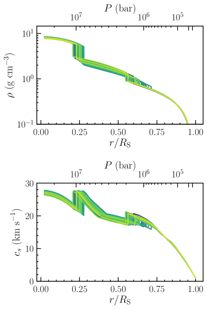
Figure 1: Saturn interior models with two-layer envelopes of varying $Y$ and $Z$ distributions, surrounding pure-$Z$ cores. Models are sampled based on $J_{2}$ and $J_{4}$ from Iess et al. (2018). Mass density (top panel) and sound speed (bottom panel) are shown as functions of the mean radii of level surfaces (bottom horizontal axes) and pressure coordinate (top horizontal axes).

The values for the gravity used for generating interior models are those of Jacobson et al. (2006), appropriately normalized to our slightly smaller adopted reference equatorial radius according to $J_{2n}^{\prime}=(a/a^{\prime})J_{2n}$. Although dramatically more precise harmonics obtained from the Cassini Grand Finale orbits will soon be published, the values of $J_{2}$ and $J_{4}$ from Jacobson et al. (2006) are already precise to a level beyond that which can be used to put meaningful constraints on the deep interior using our fourth-order theory of figures, where in practice solutions are only obtained with numerical precision at the level of $|\delta J_{2}/J_{2}|\approx|\delta J_{4}/J_{4}|\lesssim 10^{-4}$.

For the purpose of fitting the gravity field, we create models using $m_{\Omega}=0.13963$ corresponding to the 10h 39m 24s $(10.657{\rm h})$ rotation period measured from Voyager kilometric radiation and magnetic field data by Desch & Kaiser (1981). We sample interior models from a bivariate normal likelihood distribution in $J_{2}$ and $J_{4}$ using emcee (Foreman-Mackey et al., 2013) assuming a diagonal covariance for these gravity harmonics. Because the numerical precision to which our theory of figures can calculate $J_{2}$ exceeds its observational uncertainty, the former is used in our likelihood function. We take uniform priors on $Z_{1}$ and $Z_{2}$ subject to the constraint that $0<Z_{1}<Z_{2}<1$, a uniform prior on $0<Y_{1}<0.275$, and a uniform prior over $0.5\ {\rm Mbar}<P_{12}<2\ {\rm Mbar}$. The mass distributions and sound speeds for models in this sample are illustrated in Figure 1.

3 Mode eigenfrequencies and eigenfunctions

Our approach is to perform the pulsation calculation for spherical models corresponding to the converged theory of figures models, with the various material parameters defined on the mean radii $r$ of level surfaces. The influence of Saturn’s rapid rotation is accounted for after the fact using a perturbation theory that expresses the full solutions in the presence of Coriolis and centrifugal forces and oblateness in terms of linear superpositions of the solutions obtained in the non-rotating case.

For spherical models, we solve the fourth-order system of equations governing linear, adiabatic oscillations (Unno et al., 1989) using the open source GYRE stellar oscillation code suite (Townsend & Teitler, 2013). The four assumed boundary conditions correspond to the enforcement of regularity of the eigenfunctions at $r=0$ and the vanishing of the Lagrangian pressure perturbation at the planet’s surface $r=R$ (Unno et al., 1989, Section 18.1). The three-layer nature of the interior models considered in this work involve two locations at which the density and sound speed are discontinuous as a result of discontinuous composition changes (see Figure 1). Additional conditions are applied at the locations of these discontinuities; these amount to jump conditions enforcing the conservation of mass and momentum across these boundaries.

As will be discussed in Section 5, comparison with the full set of observed waves in the C ring requires $f$-modes with angular degree in the range $\ell=2-14$, and we tabulate results through for the $f$-modes through $\ell=15$.

In what follows, we adopt the convention that $m>0$ corresponds to prograde modes—those that propagate in the same sense as Saturn’s rotation—so that the time-dependent Eulerian perturbation to, e.g., the mass density corresponding to the $\ell mn$ normal mode in the planet is written as

$$\rho_{\ell mn}^{\prime}(r,\theta,\varphi,t)=\rho_{\ell mn}^{\prime}(r)Y_{\ell}^{m}(\theta,\varphi)e^{-i\sigma_{\ell mn}t},$$ (4)

where $\sigma_{\ell mn}$ is the mode frequency in the frame rotating with the planet, and $r$, $\theta$, and $\varphi$ denote radius, colatitude, and azimuth respectively. Analogous relations hold with the pressure $P$ or gravitational potential $\Phi$ in place of density. The $Y_{\ell}^{m}(\theta,\varphi)$ are the spherical harmonics, here defined in terms of the associated Legendre polynomials $P_{\ell}^{m}$ as

$$\begin{split}Y_{\ell}^{m}(\theta,\varphi)=&(-1)^{\frac{m+|m|}{2}}\left[\left(\frac{2\ell+1}{4\pi}\right)\left(\frac{(\ell-|m|)!}{(\ell+|m|)!}\right)\right]^{1/2}\\ &\quad\times P_{\ell}^{m}(\cos\theta)e^{im\varphi}.\end{split}$$ (5)

The solution for the displacement itself has both radial and horizontal components, with the total displacement vector given by

$$\begin{split}\bm{\xi}(r,\theta,\varphi,t)=&\left[\xi_{r}(r)\,\hat{r}+\xi_{h}(r)\left(\hat{\theta}\frac{\partial}{\partial\theta}+\hat{\varphi}\frac{1}{\sin\theta}\frac{\partial}{\partial\varphi}\right)\right]\\ &\quad\times Y_{\ell}^{m}(\theta,\varphi)e^{-i\sigma_{\ell mn}t}.\end{split}$$ (6)

3.1 Rotation

In reality, Saturn’s eigenfrequencies are significantly modified by the action of Saturn’s rapid rotation because of Coriolis and centrifugal forces and the ellipticity of level surfaces. We account for these following the perturbation theory given by Vorontsov & Zharkov (1981) (see also Saio 1981) and later generalized by Vorontsov (1981) to treat differential rotation, using the eigenfunctions obtained in the non-rotating case as basis functions for expressing the full solutions. In this work we calculate corrected eigenfrequencies for a range of rotation rates, treating Saturn as a rigidly rotating body.

Denoting by $\tilde{\sigma}_{\ell mn}$ the eigenfrequency obtained for the $\ell mn$ mode in the non-rotating case, we write the corrected eigenfrequency as an expansion to second order in the small parameter

$$\lambda\equiv\frac{\Omega_{\rm S}}{\tilde{\sigma}_{\ell mn}}$$ (7)

so that the corrected frequency as seen in inertial space is given by

$$\sigma_{\ell mn}=\tilde{\sigma}_{\ell mn}\left[1+\sigma_{\ell mn,1}\lambda+\sigma_{\ell mn,2}\lambda^{2}+\mathcal{O}(\lambda^{3})\right].$$ (8)

For Saturn’s $f$-modes, $\lambda\approx 0.3$ for $\ell=2$ and decreases to $\lambda\approx 0.1$ by $\ell=15$. The dimensionless factor $\sigma_{\ell mn,1}$ includes the effects of the Coriolis force and the Doppler shift out of the planet’s rotating reference frame. $\sigma_{\ell mn,2}$ includes the effects of the centrifugal force and ellipticity of the planet’s figure as a result of rotation. In the limit of slow rotation, it is appropriate to truncate the expansion at first order in $\lambda$, in which case Equation 8 reduces to the well-known correction of Ledoux (1951) in which the Coriolis force breaks the frequency’s degeneracy with respect to the azimuthal order $m$.

Expressions for $\sigma_{\ell mn,1}$ and $\sigma_{\ell mn,2}$ are obtained through the perturbation theory; in practical terms they are inner products involving the zeroth-order eigenfunctions and operators describing the Coriolis and centrifugal forces and ellipticity. Corrections related to the distortion of equipotential surfaces require knowledge of the planetary figure as a function of depth, and these are provided directly by the theory of figures as described in Section 2.1.

This formalism is constructed to retain the separability of eigenmodes in terms of the spherical harmonics $Y_{\ell}^{m}$, so that each corrected planet mode may still be uniquely specified by the integers $\ell$, $m$ and $n$ and the expressions 4 and 6 hold for the corrected eigenfunctions. Generally speaking, distinct modes whose frequencies are brought into close proximity by the perturbations from rotation may interact, yielding modes of mixed character. In the second-order theory applied to rigid rotation, selection rules limit these interactions to pairs of modes with the same $m$ and with $\ell$ differing by $-2$, $0$, or $+2$. Vorontsov & Zharkov (1981) found that for $f$- and $p$-modes with $\ell\leq 8$ these additional frequency perturbations do not exceed $0.5\%$, roughly an order of magnitude smaller than the second-order corrections themselves, and indeed generally smaller than the truncation error associated with neglecting higher-order correction terms (see below). There is thus little to be gained from incorporating mode-mode interactions given the accuracy of the present theory, but mode-mode interactions could be meaningfully taken into account in a third-order perturbation theory. The present work neglects mode-mode interactions.

Further details on the calculation of these rotation corrections are given by Marley (1990), which the present implementation follows closely. The interior density and sound speed discontinuities described above necessitate additional second-order corrections accounting for the ellipticity of these transitions and the gravitational potential perturbation felt throughout the planet as a result (Vorontsov & Zharkov, 1981, Section 5).

Equation 8 provides the mode frequency as seen in inertial space. This frequency can in turn be related to a pattern speed—the rotation rate of the full $m$-fold azimuthally periodic pattern—according to

$$\Omega_{\rm pat}=\frac{1}{m}\sigma_{\ell mn},$$ (9)

which is suitable for direct comparison with the pattern speeds observed for waves in the rings. For completeness, the mode frequency in the planet’s corotating frame is related to the frequency seen in inertial space by

$$\sigma_{\ell mn}=\sigma_{\ell mn}^{\rm corot}+m\Omega_{\rm S}$$ (10)

i.e., modes that are prograde in the planet’s frame ($m>0$) modes appear to have larger frequencies in inertial space as a result of Saturn’s rotation.

As an illustration of the relative importance of these various contributions to the modeled pattern speed, we may substitute the frequency expansion 8 into 9 to write

$$\Omega_{\rm pat}=\frac{\tilde{\sigma}_{\ell mn}}{m}+\frac{\sigma_{\ell mn,1}\Omega_{\rm S}}{m}+\frac{\sigma_{\ell mn,2}\Omega_{\rm S}^{2}}{m\tilde{\sigma}_{\ell mn}}.$$ (11)

These three contributions are shown in Figure 2, which demonstrates that the second-order rotation corrections affect the pattern speeds at the level of $\gtrsim 50\ {\rm deg\ day}^{-1}$ for modes with $\ell$ below $15$. These corrections are thus essential for comparison with the observed wave pattern speeds, whose uncertainties are no larger than approximately $0.1\ {\rm deg\ day}^{-1}$ (P.D. Nicholson, private communication).

Higher order terms in the series expansion are potentially also significant. A third-order theory would include in the expansion 11 a $\lambda^{3}$ term

$$\Omega_{\rm pat}^{(3)}\equiv\frac{\sigma_{\ell mn,3}\Omega_{\rm S}^{3}}{m\tilde{\sigma}_{\ell mn}^{2}},$$ (12)

where the nondimensional prefactor $\sigma_{\ell mn,3}$ involves significant mathematical complexity (Soufi et al., 1998; Karami, 2008). To establish an upper limit for the magnitude of third-order corrections, noting that $\left|\sigma_{\ell mn,2}\right|<\left|\sigma_{\ell mn,1}\right|$ for all modes we consider, we suppose that similarly $\left|\sigma_{\ell mn,3}\right|\leq\left|\sigma_{\ell mn,2}\right|$ and thus adopt $\left|\sigma_{\ell mn,3}\right|=\left|\sigma_{\ell mn,2}\right|$ as an upper limit. The resulting upper limits on third-order contributions to $f$-mode pattern speeds are indicated in Figure 2, which demonstrates that the truncation error associated with our second-order theory may be as large as $30\ {\rm deg\ day}^{-1}$ for $\ell=m=2$, but decaying with increasing $m$. As discussed Section 5 below, these error estimates are taken into account in our analysis to ensure that the systematic dependence of the truncation error on $m$ does not bias our estimate of Saturn’s bulk rotation rate.

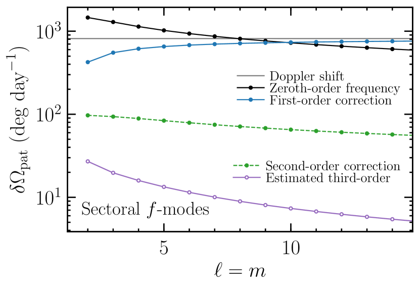
Figure 2: Magnitude of the contributions made to the modeled pattern speed by each of the four terms in Equation 11, as well as the estimate (12) for the magnitude of third-order corrections. For these prograde modes the first-order corrections (Doppler plus Coriolis; blue solid curve) take positive values, the second-order corrections (centrifugal force and ellipticity; green dashed curve) take negative values, and the estimated third-order intrinsic corrections (purple solid curve) have no assumed sign.

4 Saturnian $f$-modes in the rings

This section briefly summarizes the formalism (Marley & Porco, 1993) connecting Saturn’s nonradial oscillations with orbital resonances in the rings.

4.1 Resonance conditions

The condition for a Lindblad resonance is (Goldreich & Tremaine, 1979)

$$m(\Omega-\Omega_{\rm pat})=\pm q\kappa$$ (13)

with the upper sign corresponding an inner Lindblad resonance (ILR) and the lower sign corresponding to an outer Lindblad resonance (OLR), and with $q$ a positive integer. Taking the lower sign in Equation 13 to consider an OLR, it physically represents the condition that the perturbing pattern overtakes an orbiting ring particle once every $m/q$ epicycles. This prograde forcing in phase with the ring particles’ epicycles leads to a deposition of angular momentum that may launch a spiral density wave propagating toward the planet, assuming self-gravity is the relevant restoring force. At an ILR an orbiting particle instead overtakes the slower perturbing pattern once every $m/q$ epicycles, leading to a removal of angular momentum that may launch a spiral density wave that propagates away from the planet. Such waves are common in Saturn’s rings at mean motion resonances with Saturnian satellites.

Vertical resonances satisfy an analogous condition, namely that the perturbing pattern speed relative to the ring orbital frequency is simply related to the characteristic vertical frequency $\mu$ in the rings:

$$m(\Omega-\Omega_{\rm pat})=\pm b\mu,$$ (14)

where $b$ is a positive integer and the vertical frequency $\mu(r)$ in the ring plane can be obtained from (Shu et al., 1983)

$$\mu^{2}+\kappa^{2}=2\Omega^{2}.$$ (15)

As with Lindblad resonances, there exist both inner and outer vertical resonances (IVRs and OVRs), depending on the sign of $\Omega-\Omega_{\rm pat}$. Self-gravity waves excited at vertical resonances generally propagate in the opposite sense from those excited at Lindblad resonances, so that bending waves at IVRs propagate toward the planet and those at ILRs propagate away. IVRs are common in the rings as a result of Saturnian satellites, namely those whose inclinations provide resonant vertical forcing.

In the above, the positive integer $q$ or $b$ is sometimes referred to as the ‘order’ of the resonance. This work focuses on first-order ($q=1$ or $b=1$) resonances; higher-order resonances are possible (Marley, 2014) but the wave structures they produce may destructively interfere (P.D. Nicholson, private communication) and these resonances do not appear to need to be invoked to explain the present data (see Section 5 below). Furthermore, in what follows we limit our attention to OLRs and OVRs because in practice, the prograde $f$-modes of modest angular degree have pattern speeds that exceed $\Omega(r)$ throughout the C ring.

The orbital and epicyclic frequencies $\Omega$ and $\kappa$ for orbits at low inclination and low eccentricity can generally be written as a multipole expansion in terms of the zonal gravitational harmonics $J_{2n}$, namely

$$\Omega^{2}(r)=\frac{GM}{r^{3}}\Bigg{[}1+\sum_{n=1}^{\infty}A_{2n}J_{2n}\left(\frac{a}{r}\right)^{2n}\Bigg{]}$$ (16)

and

$$\kappa^{2}(r)=\frac{GM}{r^{3}}\Bigg{[}1+\sum_{n=1}^{\infty}B_{2n}J_{2n}\left(\frac{a}{r}\right)^{2n}\Bigg{]},$$ (17)

with the $J_{2n}$ values scaled to the appropriate reference equatorial radius $a$. The $A_{2n}$ and $B_{2n}$ are rational coefficients and are tabulated by Nicholson & Porco (1988). We use the even harmonics of Iess et al. (2018) through $J_{12}$ for the purposes of locating resonances in the ring plane, although the gravity field only affects radial locations of resonances and has no bearing on $f$-mode pattern speeds. We therefore use the latter for quantitative comparison between model $f$-modes and observed waves.

The above relations constitute a closed system allowing the comparison of planet mode frequencies to the frequencies of waves observed at resonances in the rings. In cases where we do compare resonance locations, the resonant radius for a Lindblad or vertical resonance is obtained by numerically solving Equation 13 or 14.

4.2 Which modes for which resonances?

Each planet mode can generate one of either density waves or bending waves. The type of wave that the $\ell mn$ mode is capable of driving depends on its angular symmetry, and in particular the integer $\ell-m=(0,1,2,3,\ldots)$. Modes with even $\ell-m$ are permanently symmetric with respect to the equator, and so are not capable of any vertical forcing. However, they are antisymmetric with respect to their azimuthal nodes, and so do contribute periodic azimuthal forcing on the rings. The reverse is true of modes with odd $\ell-m$, whose perturbations are antisymmetric with respect to the equator and so do contribute periodic vertical forcing on ring particles. Meanwhile their latitude-average azimuthal symmetry as experienced at the equator prevents them from forcing ring particles prograde or retrograde.

In what follows, we restrict our attention to prograde $f$-modes, namely the normal modes with $m>0$ and $n=0$. Acoustic modes with overtones ($n>0$; $p$-modes) are not considered because that they contribute only weakly to the external potential perturbation due to self-cancellation in the volume integral of the Eulerian density perturbation; see Equation A15. We further limit our consideration to prograde modes because while $f$-modes that are retrograde in the frame rotating with the planet can in principle be boosted prograde by Saturn’s rotation (see Equation 10), we find that the resulting low pattern speeds ($\lesssim 500\ {\rm deg\ day}^{-1}$) would place any Lindblad or vertical resonances beyond the extent of even the A or B rings. Finally, azimuthally symmetric ($m=0$) modes do not lead to Lindblad or vertical resonances.

5 Results for rigid rotation

Figure 3 summarizes the OLR and OVR locations of prograde model Saturn $f$-modes with $\ell-m$ between zero and five, together with locations of 17 inward-propagating density waves and four outward-propagating bending waves observed in Cassini VIMS data. A visual comparison in this diagram provides a strong indication that the $f$-modes are responsible for the majority of the wave features shown. In particular, we can make unambiguous identifications for the $f$-modes at the origin of 10 of the 17 density waves, and all four of the bending waves; these visual identifications are summarized in Table 1.

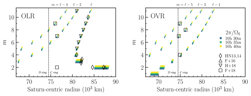
Figure 3: Locations of resonances with our model Saturn’s $f$-modes (colorful horizontal spans) and wave features observed in Saturn’s C ring using stellar occultations in Cassini VIMS data (open symbols; see references in Table 1). The number of spiral arms $m$ (or equivalently, the azimuthal order of the perturbing planet mode) is shown versus distance from Saturn’s center in the ring plane. Left panel: Outer Lindblad resonances, which can excite inward-propagating spiral density waves in the rings. The three roughly vertical model sequences correspond to modes with $m=\ell$, $m=\ell-2$, and $m=\ell-4$ from right to left. The three observed $m=3$ density waves are offset vertically for clarity. Right panel: Outer vertical resonances, which can excite outward-propagating bending waves in the rings. The three vertical model sequences correspond to $m=\ell-1$, $m=\ell-3$, and $m=\ell-5$ from right to left. Model resonances are colored by the assumed Saturn rotation rate as described in the legend; the resonances indicated for each rotation rate are slightly offset vertically for clarity.

The remaining seven density waves at $m=2$ and $m=3$ exhibit frequency splitting that is likely attributable to mixing with deep $g$-modes as proposed by Fuller (2014), and which our model, lacking a stable stratification outside the core, does not attempt to address. We thus omit all $m=2$ and $m=3$ waves from the quantitative analysis that follows, although we note that the predicted $\ell=m=2$ and $\ell=m=3$ $f$-mode OLR locations do generally coincide with the locus of observed density waves for these $m$ values, the sole exception being the close-in W76.44. This wave was only recently detected in VIMS data (French et al., 2018), and while coupling with deep $g$-modes is a possible interpretation (E. Dederick, private communication), this wave may be particularly challenging to explain due to its large splitting from the other three $m=2$ waves. We also note that the frequency and $m$ value of the outermost $m=2$ density wave in the ringlet within the Maxwell gap (French et al., 2016) were predicted by Fuller (2014).

As discussed in Section 3, the density and sound speed discontinuities inherent to the three-layer interior structures assumed for Saturn affect the $f$-mode frequencies. Their effect is strongest for the lowest-degree $f$-modes, which have significant amplitude at these deep transitions. This is evident in Figure 3 in the considerable spread of predicted locations for resonances with the $\ell=\{2,3\}$ $f$-modes. By $\ell\gtrsim 4$ the $f$-modes have low enough amplitudes at these deep density transitions that their frequencies are not strongly affected.

The model $f$-modes whose resonance locations coincide with the remainder of the observed waves contain a striking range of radial and latitudinal structures, including the rest of the sectoral $(\ell=m)$ sequence up to $\ell=m=10$, as well as seven non-sectoral ($\ell\neq m$) modes with $\ell-m=\{1,2,3,4,5\}.$ These waves are evidently the result of time-dependent tesseral harmonics resulting from Saturn’s nonradial oscillations.

Although general agreement for these is evident at the broad scale of Figure 3, the observed wave pattern speeds are known to a precision better than $0.1\ {\rm deg\ day}^{-1}$ for the weakest waves yet measured (P. D. Nicholson, private communication). This high precision warrants a closer inspection of the pattern speed residuals with respect to our predictions. What follows in the remainder of this section is an analysis of these residuals and their dependence on the assumed interior model and rotation rate.

Table 1: C ring wave patterns and Saturn $f$-mode associations

			Observed				Model prediction
Reference	Wave	Symbol	$m$	$\Omega_{\rm pat}$	Type		$\ell$	$\Omega_{\rm pat}$	$\Delta\Omega_{\rm pat}\ ({\rm model-obs})$
F+18	W76.44	$\square$	2	2169.3	OLR		—	—	—
HN13	W84.64	$\diamondsuit$	2	1860.8	OLR		—	—	—
HN13	W87.19	$\diamondsuit$	2	1779.5	OLR		—	—	—
F+16	Maxwell	$\bigtriangleup$	2	1769.2	OLR		—	—	—
HN13	W82.00	$\diamondsuit$	3	1736.7	OLR		—	—	—
HN13	W82.06	$\diamondsuit$	3	1735.0	OLR		—	—	—
HN13	W82.21	$\diamondsuit$	3	1730.3	OLR		—	—	—
HN13	W80.98	$\diamondsuit$	4	1660.4	OLR		4	$1657.87\textup{--}1673.41$	$-2.49\textup{--}13.05$
H+18	W81.02a	$\bigtriangledown$	5	1593.6	OLR		5	$1592.08\textup{--}1596.05$	$-1.54\textup{--}2.43$
H+18	W81.43	$\bigtriangledown$	6	1538.2	OLR		6	$1537.10\textup{--}1539.51$	$-1.13\textup{--}1.28$
H+18	W81.96	$\bigtriangledown$	7	1492.5	OLR		7	$1491.73\textup{--}1493.72$	$-0.73\textup{--}1.26$
F+18	W76.46	$\square$	7	1657.7	OLR		9	$1655.86\textup{--}1657.35$	$-1.86\textup{--}-0.37$
H+18	W82.53	$\bigtriangledown$	8	1454.2	OLR		8	$1453.93\textup{--}1455.23$	$-0.30\textup{--}1.00$
H+18	W83.09	$\bigtriangledown$	9	1421.8	OLR		9	$1421.83\textup{--}1422.55$	$-0.01\textup{--}0.71$
F+18	W76.02	$\square$	9	1626.5	OLR		13	$1626.48\textup{--}1627.46$	$-0.02\textup{--}0.96$
HN14	W83.63	$\diamondsuit$	10	1394.1	OLR		10	$1394.03\textup{--}1394.71$	$-0.03\textup{--}0.65$
H+18	W81.02b	$\bigtriangledown$	11	1450.5	OLR		13	$1451.53\textup{--}1453.07$	$1.04\textup{--}2.58$
F+18	W74.93	$\square$	4	1879.6	OVR		5	$1871.22\textup{--}1875.42$	$-8.42\textup{--}-4.22$
F+18	W74.67	$\square$	7	1725.8	OVR		10	$1723.99\textup{--}1725.28$	$-1.77\textup{--}-0.48$
F+18	W76.24	$\square$	8	1645.4	OVR		11	$1644.89\textup{--}1645.81$	$-0.54\textup{--}0.38$
F+18	W74.94	$\square$	9	1667.7	OVR		14	$1667.72\textup{--}1668.85$	$-0.01\textup{--}1.12$

5.1 Saturn’s seismological rotation rate

Saturn’s bulk rotation rate has to date been deduced from a combination of gravity field and radiometry data from the Pioneer, Voyager and Cassini spacecrafts (e.g., Desch & Kaiser 1981, Gurnett et al. 2005, Giampieri et al. 2006, Anderson & Schubert 2007). Along different lines, Helled et al. (2015) optimized interior models to the observed gravity field and oblateness to extract the rotation rate. Since we have demonstrated that the frequencies of Saturnian $f$-modes depend strongly on $\Omega_{\rm S}$ through the influence of the Coriolis and centrifugal forces and the ellipticity of level surfaces, a natural question is, what interior rotation rate is favored by the waves detected so far that appear to be associated with modes in Saturn’s interior?

Given an observed C ring wave with a pattern speed $\Omega_{\rm pat}^{\rm obs}$ that appears to be associated with a predicted Saturn model $f$-mode resonance with pattern speed $\Omega_{\rm pat}$ and azimuthal order matching the observed number of spiral arms $m$, we calculate the pattern speed residual $\Delta\Omega_{\rm pat}\equiv\Omega_{\rm pat}-\Omega_{\rm pat}^{\rm obs}$. For each Saturn interior model and rotation rate considered, we calculate a weighted root-mean-square (RMS) value of $\Delta\Omega_{\rm pat}$ over the set of mode-wave pairs according to

$${\rm RMS}\ \Delta\Omega_{\rm pat}\equiv\left[\sum_{i}w_{i}\left|\Delta\Omega_{\rm pat,\,i}\right|^{2}\right],$$ (18)

where the weights $w_{i}$ are assigned in inverse proportion with the maximum magnitude of third-order corrections as described in Section 3.1, the weights sum to unity, and $i$ indexes the set of waves that we have identified with Saturn $f$-modes, namely those with $\ell$ values and model pattern speeds listed in Table 1. The resulting curves are shown in Figure 4 for rotation periods between $10{\rm h}\,30{\rm m}$ and $10{\rm h}\,42{\rm m}$. The relation between ${\rm RMS}\ \Delta\Omega_{\rm pat}$ and $\Omega_{\rm S}$ always exhibits a distinct minimum, owing to the strongly correlated response of the $f$-mode frequencies to varying $\Omega_{\rm S}$. In particular, the predicted pattern speeds increase uniformly with faster Saturn rotation.

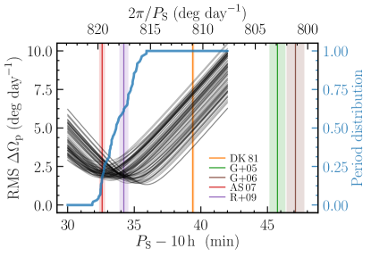
Figure 4: Saturn’s rotation rate from fits to the set of observed C ring waves identified with Saturnian $f$-modes. RMS pattern speed residuals across the full set of waves are shown as a function of Saturn’s assumed rotation rate. Each black curve corresponds to a single interior model from the sample shown in Figure 1. The thick blue curve shows the cumulative distribution of rotation periods minimizing the weighted RMS pattern speed residuals for each model; its median and 5%/95% quantiles are given in Section 5.1. Vertical lines with shaded errors indicate Saturn rotation rates in the literature, references to which are given in the text. For visual clarity the Helled et al. (2015) result of $10{\rm h}\,32{\rm m}\,(45\pm 46){\rm s}$ referred to in the text is omitted from the diagram.

The optimal Saturn rotation period depends on the interior model chosen, as does the quality of that best fit: interior models favoring longer rotation periods generally achieve a slightly better bit. To account for this in our esimate of Saturn’s bulk rotation period, we weight the optimized rotation period from each interior model in inverse proportion to the value of ${\rm RMS}\ \Delta\Omega_{\rm pat}$ obtained there. The cumulative distribution of rotation rates resulting from our sample of interior models is shown in Figure 4. This distribution may be summarized as $P_{\rm S}=10.561^{+0.031}_{-0.022}\,{\rm h}=10{\rm h}\,33{\rm m}\,38{\rm s}^{+1{\rm m}\,52{\rm s}}_{-1{\rm m}\,19{\rm s}}$ where the leading value corresponds to the median and the upper (lower) error corresponds to the 95% (5%) quantile. This may be expressed in terms of a pattern speed as $2\pi/P_{\rm S}=818.13^{+2.41}_{-1.70}\,{\rm deg\ day}^{-1}$.

Although these seismological calculations vary the assumed rotation rate, the underlying interiors randomly sampled against $J_{2}$ and $J_{4}$ using the theory of figures as described in Section 2.1 assumed the Desch & Kaiser (1981) Voyager rate, in principle an inconsistency of the model. As a diagnostic we generate a new sample from the gravity field, but adopting $m_{\Omega}=0.14201$ consistent with the 10.561h median rotation period derived here. Repeating the remainder of this analysis we find a very similar distribution of optimal rotation periods, the median shifting to longer periods by approximately one minute as a result of the slightly different interior mass distributions obtained. The frequencies of the $f$-modes themselves are inherently more sensitive to Saturn’s assumed rotation rate than are the low-order gravity harmonics $J_{2}$ and $J_{4}$, a consequence of the $f$-modes extending to relatively high $m$ where Saturn’s rotation imparts a larger fractional change to the frequency (see Figure 2).

5.2 Is rigid rotation adequate?

The lack of any perfect fit among the range of interior structures and rotation rates we have considered is evident in Figure 4, where the RMS pattern speed residuals reach approximately 1.2 ${\rm deg\ day}^{-1}$ at best, an order of magnitude larger than the typical observational uncertainty of approximately $0.1\ {\rm deg\ day}^{-1}$ associated with even the weakest waves we compare to here (P.D. Nicholson, private communication). The absolute residuals are shown mode by mode in Figure 5, including the full span of residuals obtained over the sample of interior models, each one evaluated at its optimal rotation rate. Points lie on both sides of zero by construction, but again no model provides an entirely satisfactory fit.

First, it is notable that the model pattern speed covariance (the diagonal elements of which set the vertical spans in the residuals of Figure 5) varies so strongly and non-monotonically with $m$. This can be understood as a consequence of the tradeoff between the decreasing zeroth-order frequency and the increasing contribution from the first-order rotation correction with increasing $\ell$, as can be seen from Figure 2 for the sectoral modes. At high $\ell$, the zeroth-order frequency loses out to the first-order correction. Since the latter is proportional to $\Omega_{\rm S}$, the overall pattern speeds vary more strongly with rotation than at intermediate $\ell$. At low $\ell$, where the frequency is dominated by the zeroth order contribution and so rotation plays a smaller role, the large model covariance is due mostly to sensitivity to the locations of the core boundary and envelope transition, sensitivity that decays rapidly with increasing $\ell$ as modes are confined increasingly close to the planet’s surface.

A significant observational development has been made by Hedman et al. (2018) in their detection of density waves corresponding to the full set of Saturn’s sectoral $f$-modes from $\ell=m=2$ up to $\ell=m=10$, constituting frequency measurements for modes that possess the same latitudinal symmetry but sample an uninterrupted sequence of depths within Saturn. On the other hand, the non-sectoral ($\ell\neq m$) $f$-mode waves reported by Hedman et al. (2018) and French et al. (2018) extend the detections up to $\ell=14$ but also importantly sample a variety of latitudinal structures inside the planet by virtue of the range in their values of $\ell-m$. Thus in principle the available modes serve to constrain differential rotation inside Saturn.

With this in mind, the second panel of Figure 5 is a valuable illustration because any strong differential rotation as a function of depth or latitude would generally manifest as systematic trends in the residuals $\Delta\Omega_{\rm pat}$ as a function of $\ell$ or $\ell-m$ respectively when referred to the rigid model. Instead, the residuals exhibit no obvious systematic dependence on $\ell$, although small systematic departures as a function of $\ell-m$ may indicate the presence of differential rotation as a function of latitude. In particular, in each of the four cases where two modes belonging to the same multiplet have been observed ($\ell=5,\ 9,\ 10,\ {\rm and}\ 13$), the two frequencies are offset by between 1 and 5 deg day^-1.

More firm conclusions regarding the presence or strength of differential rotation are not possible given the present theoretical accuracy limitations discussed in Section 3.1. A more accurate treatment of rotation effects could potentially increase the predicted pattern speeds of the low-$m$ modes by as many as tens of $\rm deg\ day^{-1}$ (see Figure 2) which could produce a spectrum consistent with a spin frequency increasing by several percent toward the planet’s surface. Indeed, this systematic uncertainty motivates the weighted fit that we carry out in our estimate of Saturn’s bulk rotation in Section 5.1. Ultimately a more accurate perturbation theory, or else non-perturbative methods (e.g., Mirouh et al., 2018), will be required to fully interpret the implications for differential rotation inside Saturn.

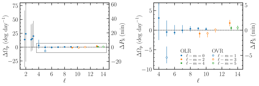
Figure 5: Pattern speeds residuals (predicted minus observed) for models each calculated at their optimal Saturn rotation period. Left panel: All residual frequencies, including those for the $m=2$ and $m=3$ sectoral $f$-modes for which identification with specific $m=2$ or $m=3$ density waves is not possible. For these modes residuals are shown with respect to each of the nearby density waves having the correct $m$ value. The domain of the right panel is indicated. Right panel: Frequency residuals for the 14 waves identified with Saturn $f$-modes and used to constrain Saturn’s rotation. Circular markers are for one interior model randomly chosen from our sample, while vertical lines show the span of residuals obtained for the full sample. These vertical spans thus indicate the amount of freedom available from the low-order gravity field as applied to three-layer Saturn models, when the rotation rates are tuned using the seismology. Note that these spans do not represent random uncertainties because the residuals for the various modes are highly correlated. The vertical axis at right expresses the residuals in terms of minutes of Saturn rotation, i.e., the degree to which Saturn would need to be spun up or down to fit a given wave’s observed pattern speed. Four pairs of modes that are members of same-$\ell$ multiplets are evident (see discussion in Section 7); the pairs with $\ell=9$, 10, and 13 are slightly offset horizontally for clarity.

6 Strength of forcing

The adiabatic eigenfrequency calculation that forms the basis for this work provides no information about excitation or damping of normal modes, processes which have yet to be adequately understood in the context of gas giants.

Stochastic excitation of modes by turbulent convection such as in solar-type oscillations is one obvious candidate for Jupiter and Saturn, where convective flux dominates the intrinsic flux in each planet. However, the expectation from simple models for resonant coupling of $f-$ and $p-$modes with a turbulent cascade of convective eddies (e.g., Markham & Stevenson (2018) following the theory of Kumar (1997)) is that these modes are not excited to the amplitudes necessary to provide the mHz power excess that Gaulme et al. (2011) attributed to Jovian $p$-modes.

Recent work from Dederick & Jackiewicz (2017) demonstrated that a radiative opacity mechanism is not able to drive the Jovian oscillations, although they noted that driving by intense stellar irradiation is possible for hot Jupiters. Dederick et al. (2018) and Markham & Stevenson (2018) each focused on water storms as a mode excitation mechanism, finding this too insufficient for generating a power spectrum akin to that reported by Gaulme et al. (2011). Markham & Stevenson (2018) further demonstrated that deeper, more energetic storms associated with the condensation of silicates were viable.

In lieu of a complete understanding of the amplitudes of acoustic modes in gas giants, we simply adopt equal mode energy across the f-mode spectrum following

$$E_{\ell mn}\propto\sigma_{\ell mn}^{2}|\bm{\xi}|^{2}=\rm constant,$$ (19)

corresponding to the “strong coupling” case cited by Marley & Porco (1993). Less efficient coupling of the turbulence with the $f$-modes could result in a steeper decline of equilibrium mode energy with frequency; Marley & Porco (1993) adopted $E_{\ell mn}\propto\sigma_{\ell mn}^{-13/2}$ as a limiting case.

Because the scaling relation 19 is only a proportionality, it remains to set an overall normalization by choosing the amplitude of a single mode. Marley & Porco (1993) proposed that the $\ell=m=2$ $f$-mode OLR is the origin of the Maxwell gap, and accordingly anchored their amplitude spectrum by assuming that this mode had an amplitude sufficient to produce the OLR torque $T^{L}/\Sigma\sim 10^{16}\ {\rm cm}^{4}\ {\rm s}^{-2}$ necessary to open a gap (Rosen et al., 1991a). The corresponding displacement amplitude was of order 100 cm; we follow suit and adopt 100 cm as the amplitude of this mode.

In what follows we normalize our $f$-mode eigenfunctions in accordance with the amplitude estimate of Equation 19 and derive the resulting torques applied at OLRs and OVRs. While this amplitude law is but one of many plausible scenarios, any similar scaling relation will yield the same general dependence of Lindblad and vertical torques on $\ell$, $m$, and position in the ring plane. In particular, the magnitudes of the torques decline monotonically with $\ell$ for a given $\ell-m$, and also with $\ell-m$ for a given $m$. This is sufficient for a basic prediction of the relative strengths of waves at the $f$-mode resonances calculated here, which will allow us to identify locations that may harbor hitherto-undetected waves.

6.1 Torques and detectability

In deriving the magnitudes of torques applied at ring resonances we follow the approach of Marley & Porco (1993). In a ring of surface mass density $\Sigma$, the linear torque applied at a Lindblad resonance is (Goldreich & Tremaine, 1979)

$$T_{\ell mn}^{L}=-\frac{m\pi^{2}\Sigma}{\mathscr{D}_{L}}(2m+\ell+1)\left(\Phi_{\ell mn}^{\prime}\right)^{2},$$ (20)

where

$$\begin{split}\mathscr{D}_{L}=&-\left(3-\frac{9}{2}J_{2}\left(\frac{a}{r_{L}}\right)^{2}\right)\Omega^{2}(1\mp m)\\ &+\frac{21}{2}J_{2}\left(\frac{a}{r_{L}}\right)^{2}\Omega^{2}+\mathcal{O}(J_{2}^{2},J_{4})\end{split}$$ (21)

and $\Phi_{\ell mn}^{\prime}$ is the magnitude of the perturbation to the gravitational potential caused by the $\ell mn$ mode, evaluated at the Lindblad resonance $r=r_{L}$ in the ring plane $\cos\theta=0$. Similarly the linear torque applied at a vertical resonance $r=r_{V}$ is (Shu et al., 1983; Marley & Porco, 1993)

$$T_{\ell mn}^{V}=\frac{m\pi^{2}\Sigma}{\mathscr{D}_{V}}\left(\frac{d\Phi_{\ell mn}^{\prime}}{d\theta}\right)^{2},$$ (22)

where

$$\begin{split}\mathscr{D}_{V}=&-\left(3+\frac{9}{2}J_{2}\left(\frac{a}{r_{V}}\right)^{2}\right)\Omega^{2}(1\mp m)\\ &-\frac{21}{2}J_{2}\left(\frac{a}{r_{V}}\right)^{2}\Omega^{2}+\mathcal{O}(J_{2}^{2},J_{4})\end{split}$$ (23)

and $({d\Phi_{\ell mn}^{\prime}}/{d\theta})$ is to be evaluated at the vertical resonance $r=r_{V}$ and $\cos\theta=0$. In the expressions for $\mathscr{D}_{L}$ and $\mathscr{D}_{V}$ the upper (lower) signs correspond to inner (outer) Lindblad or vertical resonances, as in Equations 13 and 14. An expression for $\Phi_{\ell mn}^{\prime}$ is derived as in Marley & Porco (1993); this is reproduced in Appendix A for completeness. These expressions rely on integrals of the Eulerian density perturbation $\rho_{\ell mn}^{\prime}$ over the volume of the planet. While accuracy to second order in Saturn’s smallness parameter $m_{\Omega}$ would demand that this density eigenfunction include second-order corrections from the perturbation theory described in Section 3.1, the fact that only an order of magnitude calculation of the torques is required for the present purpose leads us to simply calculate these using the zeroth-order density eigenfunctions.

To illustrate which modes are likely to excite the strongest ring features, Figure 6 summarizes the torques applied by the $f$-modes at OLRs and OVRs in the C and D rings assuming mode amplitudes follow equipartition per Equation 19. Because the torques (Equations 20 and 22) are proportional to ring surface mass density $\Sigma$, itself strongly variable across the rings at a variety of spatial scales, we instead plot the normalized torques $T_{L}/\Sigma$ and $T_{V}/\Sigma$. These are straightforward quantities to calculate even with imperfect knowledge of the mass density itself. When comparing to detected wave patterns should be kept in mind that $\Sigma$ can play an important role in whether a given wave is likely to be driven to detectable amplitudes.

Saturnian waves can also be obscured by more prominent eccentric features, such as those associated with satellite resonances. Of particular importance is the strong Titan 1:0 apsidal resonance, which Nicholson et al. (2014) studied in Cassini radio and stellar occultations and found responsible for driving the $m=1$ wave in the Titan/Colombo ringlet (77,879 km) and also dozens of other $m=1$ features from 74,000-80,000 km. Their test-particle model (cf. their Figure 19) predicts maximum radial deviations in excess of 100 m as much as 3,500 km away from that resonance, posing a serious challenge for the reconstruction of weaker wave features from stellar occultation profiles obtained at different phases. This substantial region of the C ring thus may be concealing waves driven at Saturn resonances, and Figure 6 accordingly indicates the region where the maximum radial deviations are larger than 300 m according to the model of Nicholson et al. (2014).

For context, the torques associated with four satellite resonances that open gaps or launch waves in the C ring are also shown in Figure 6. Prometheus 2:1 ILR opens a gap in the C ring while the Mimas 4:1 ILR launches a wave. The Mimas 3:1 IVR opens a gap, while the Titan -1:0 nodal resonance launches a wave. Estimates for the strengths of these satellite torques are taken from Rosen et al. (1991a, b) and Marley & Porco (1993).

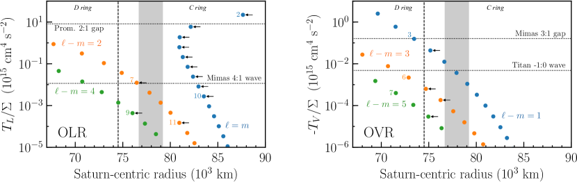
Figure 6: Strengths of torques per surface mass density exerted on the C and D rings by model Saturnian $f$-modes, with amplitudes assigned according to equal energy per mode following Equation 19. Model points (filled circles; shown for one randomly drawn interior model) are colored by their value of $\ell-m$. Arrows highlight model $f$-modes that we have identified with observed waves as in Table 1. The grey shaded region in both panels represents the region where maximum radial variations in ring orbits caused by the Titan 1:0 apsidal ILR exceed 300 m, making the detection of wave features more difficult; see Section 6. A subset of resonances have been labeled to their left by their azimuthal wavenumber $m$ for ease of identification. Torques associated with waves or gaps at example satellite ILRs or IVRs in the C ring are indicated with dotted horizontal lines.

6.1.1 Conspicuously missing waves?

Inspection of Figure 6 reveals a few $f$-mode resonances that this simple excitation model predicts to experience strong forcing, but where no waves have yet been detected. Four of the OLRs with $m=\ell-2$ have normalized torques predicted to be greater than that of the detected $(\ell,m)=(13,11)$ OLR. The most obvious of these is the $(8,6)$ OLR, which this model predicts to lie at 74,940 km, happening to be almost exactly coincident with the detected W74.93 and W74.94 OVR features (French et al., 2018). The fact that these OVR waves apparently dominate the signal at this position betrays some tension with the spectrum of amplitudes we have assumed, which predicts W74.93 and W74.94 to have torques one to three orders of magnitude lower than that predicted for the $(8,6)$ OLR. Given the close proximity of these resonances, an appeal to the spatial dependence of $\Sigma$ seems unlikely to resolve this tension.

Of the remaining $m=\ell-2$ OLRs stronger than $(13,11)$, none among $(10,8)$, $(11,9)$, or $(12,10)$ have had associated wave detections. This may be attributable to strong perturbations from the Titan apsidal resonance as discussed above. Among the predicted $m=\ell-4$ resonances, the $(12,8)$ OLR at 74,556 km is quite close to the inner boundary of the C ring where there are a series of gaps that have yet to be fully understood. Falling in such a gap could render such a resonance unobservable, although within the model uncertainty, this resonance could lie between the gaps or on gap edges.

As for the OVRs, the only resonances that yield waves that have been detected so far in the C ring are the four that fall closest to Saturn, and indeed the strongest predicted waves in each $\ell-m$ have been observed. It warrants closer attention that three of the four strongest OVRs predicted in the C ring have not been associated with any wave feature, while waves have been observed at what should be weaker OVRs with $\ell-m=3$ and $\ell-m=5$. These three “missing waves” correspond to the $(\ell,m)=(6,5)$, $(7,6)$, and $(8,7)$ Saturn $f$-modes. Because of their location, it is possible that these waves are present but obscured by the Titan apsidal resonance.

To aid in the search for Saturnian resonances in the C ring, Table 2 lists the pattern speeds of all model OLRs and OVRs in the C ring with predicted torques comparable to or larger than than the smallest predicted torque associated with a wave that has already been observed. Likewise, Table 3 reports resonances predicted to lie in the D ring, although it is not clear whether any wave patterns there will ultimately be detectable given the ring’s faintness.

Table 2: Predicted OLRs and OVRs in the C ring without associated wave detections

$\ell$	$m$	Type	$\Omega_{\rm pat}\ (\rm deg\ day^{-1})$	Remark (see Section 6)
11	11	OLR	$1368.5\textup{--}1371.5$
12	12	OLR	$1346.9\textup{--}1349.7$
13	13	OLR	$1327.7\textup{--}1330.1$
8	6	OLR	$1742.1\textup{--}1747.6$	Coincident with W74.93, W74.94
10	8	OLR	$1586.9\textup{--}1591.0$	Near Titan apsidal
11	9	OLR	$1532.9\textup{--}1536.4$	Near Titan apsidal
12	10	OLR	$1488.4\textup{--}1491.6$
14	12	OLR	$1419.3\textup{--}1421.8$
12	8	OLR	$1695.6\textup{--}1699.5$	Among gaps
14	10	OLR	$1568.6\textup{--}1571.6$	Near Titan apsidal
15	11	OLR	$1521.4\textup{--}1524.1$	Near Titan apsidal
6	5	OVR	$1737.0\textup{--}1743.6$	Near Titan apsidal
7	6	OVR	$1646.4\textup{--}1652.1$	Near Titan apsidal
8	7	OVR	$1578.0\textup{--}1582.8$
9	8	OVR	$1523.9\textup{--}1528.1$
10	9	OVR	$1479.8\textup{--}1483.5$
11	10	OVR	$1443.0\textup{--}1446.3$
12	9	OVR	$1581.1\textup{--}1584.6$	Near Titan apsidal
13	10	OVR	$1530.1\textup{--}1533.1$	Near Titan apsidal
15	10	OVR	$1604.7\textup{--}1607.6$

Note. — Pattern speeds can be mapped to physical locations given Saturn’s equatorial radius and $J_{2n}$ using the relations in Section 4.1.

Table 3: Predicted OLRs and OVRs in the D ring

$\ell$	$m$	Type	$\Omega_{\rm pat}\ (\rm deg\ day^{-1})$
5	3	OLR	$2314.3\textup{--}2324.3$
6	4	OLR	$2034.3\textup{--}2042.2$
7	5	OLR	$1861.1\textup{--}1867.6$
9	5	OLR	$2063.1\textup{--}2069.4$
10	6	OLR	$1901.5\textup{--}1906.8$
11	7	OLR	$1784.6\textup{--}1789.0$
2	1	OVR	$3359.2\textup{--}3400.7$
3	2	OVR	$2423.7\textup{--}2433.4$
4	3	OVR	$2061.8\textup{--}2070.8$
7	4	OVR	$2177.3\textup{--}2185.2$
8	5	OVR	$1968.1\textup{--}1974.5$
9	6	OVR	$1826.1\textup{--}1831.4$
11	6	OVR	$1970.5\textup{--}1975.6$
12	7	OVR	$1841.5\textup{--}1845.9$
13	8	OVR	$1743.8\textup{--}1747.5$

7 Discussion

This work offers interpretations for the set of inward-propagating density waves and outward-propagating bending waves observed in Saturn’s C ring in terms of resonances with Saturnian $f$-modes. It also demonstrates that Saturn’s rotation state is of critical importance for Saturn ring seismology, a fact made evident by the systematic mismatch with the observed pattern speeds of these waves obtained assuming that Saturn rotates rigidly at the Voyager System III magnetospheric period of Desch & Kaiser (1981) or slower (see Figure 4). The interior configurations considered to arrive at this conclusion accounted somewhat generously for the freedom in the low-order gravity field, because the likelihood function used to obtain our posterior distribution of interior models assumed an inflated variance on $J_{2}$ to accord with the numerical precision of our theory of figures implementation (see Section 2.1). Because the resulting distribution included a diversity of heavy element and helium distributions, envelope transition locations, and core masses, the seismology suggests a tension with the Voyager rotation rate commonly assumed for Saturn’s interior that different three-layer interior models seem unlikely to resolve. This conclusion based on the ring seismology adds support to the notion that periodicities in Saturn’s magnetospheric emission (e.g., Desch & Kaiser, 1981; Gurnett et al., 2005; Giampieri et al., 2006) may not be consistently coupled to the rotation of Saturn’s interior (e.g., Gurnett et al., 2007; Read et al., 2009).

The present model is potentially oversimplified in two major ways. First, the model is not suited to address the close multiplets of waves observed to have the same azimuthal wavenumber $m$, namely the multiplets of waves in the C ring with $m=2$ and $m=3$. The bulk of these seem naturally explained by the model of Fuller (2014), wherein avoided crossings between the $f$-modes and deep $g$-modes of higher angular degree give rise to a number of strong perturbations with the same $m$ value. However, in the wealth of new OLR and OVR wave patterns that have been measured from increasingly low signal to noise VIMS data since Hedman & Nicholson (2014), it seems that only two waves add to the mixed-mode picture, both with $m=2$: the close-in W76.44 wave, and the Maxwell ringlet wave whose frequency and $m$ number were predicted by Fuller (2014). The $f$-modes of higher angular degree have less amplitude in the deep interior and so are less likely to undergo degenerate mixing with any deep $g$-modes strongly. Indeed, there is not yet any direct evidence for $f$-modes with $\ell>3$ undergoing avoided crossings with deep $g$-modes, although the outlying $(5,4)$ OVR warrants closer scrutiny in the mixed-mode context.

The second major simplification of the present model is the assumption that Saturn rotates rigidly. While upper limits can be established for the depth of shear in Jupiter or Saturn’s envelopes on magnetohydrodynamic grounds (Liu et al., 2008; Cao & Stevenson, 2017), evidence gathered from spacecraft indicate that zonal wind patterns do penetrate to significant depths (Smith et al., 1982; Kaspi et al., 2018). It has been proposed that the insulating molecular regions of these planets may be rotating differentially on concentric cylinders (Busse, 1976; Ingersoll & Pollard, 1982; Ingersoll & Miller, 1986), the zonal winds being the surface manifestation of these cylinders of constant angular velocity. The mode identifications made in Section 5 and Table 1 reveal that the seismological dataset now samples a variety of radial (via the angular degree $\ell$) and latitudinal (via the latitudinal wavenumber $\ell-m$) structures within Saturn and so should strongly constrain differential rotation in Saturn’s interior. If our rigid model systematically underpredicted $f$-mode frequencies toward high $\ell$, this would indicate that Saturn’s outer envelope rotates faster than the bulk rotation. Such a result would be qualitatively consistent with the expectation for rotation on cylinders or an eastward equatorial jet that extends to significant depth, as well as with the rotation profiles that Iess et al. (2018) deduced from the Cassini Grand Finale gravity orbits. As discussed in Section 5.2, the lack of any such obvious systematic dependence of wave pattern speed residuals on $\ell$ (see Figure 5) offers a preliminary indication that Saturn does not experience strong differential rotation as a function of radius within the volume sampled by the $\ell\geq 4$ $f$-modes considered in this analysis, although we emphasize that the inclusion of higher order rotation corrections is necessary to confirm this.

The modes identified here also contain four instances of a pair of modes belonging to the same multiplet, i.e., a pair described by the same angular degree $\ell$ but different azimuthal order $m$. This carries significance for the prospect of deducing Saturn’s rotation profile from the frequency splitting within each multiplet, although the important centrifugal forces and ellipticity due to Saturn’s rapid rotation complicates the picture compared to the first-order rotation kernels commonly applied to helioseismology (Thompson et al., 2003) and asteroseismology (e.g., Beck et al., 2012). The frequency offsets that remain between modes with the same $\ell$ but different $\ell-m$ may point to a latitude-dependent spin frequency, although the manner in which this would fit in with a radius-independent spin frequency is unclear. Quantitative constraints on differential rotation via the $f$-modes awaits future work.

8 Conclusions

We have presented new Saturn interior models and used them to predict the frequency spectrum of Saturn’s nonradial acoustic oscillations. Comparison with waves observed in Saturn’s C ring through Cassini VIMS stellar occultations reveals that the majority of these waves that are driven at frequencies higher than the ring mean motion are driven by Saturn’s fundamental acoustic modes of low to intermediate angular degree $\ell$.

The frequencies of Saturn’s $f$-modes probe not only its interior mass distribution, but also its rotation state, especially those modes of higher $\ell$. We used the frequencies of the observed wave patterns to make a seismological estimate of Saturn’s rotation period assuming that it rotates rigidly. Using these optimized models, we proposed that small but significant residual signal in the frequencies of the observed waves as a function of $\ell$ suggests that Saturn’s outer envelope may rotate differentially, although we are unable to draw quantitative conclusions given the accuracy with which the present theory accounts for rotation in predicting the $f$-mode frequencies.

Saturn ring seismology is an interesting complement to global helioseismology, ground-based Jovian seismology, and asteroseismology of solar-type oscillators. Because the rings are coupled to the oscillations purely by gravity, they are fundamentally sensitive to the modes without nodes in the density perturbation as a function of radius, and the observation of modes from $\ell=2$ to $\ell\sim 15$ stands in contrast with helioseismology where the vast majority of detected modes are acoustic overtones ($p$-modes) and $f$-modes only emerge for $\ell\gtrsim 100$ (e.g., Larson & Schou, 2008). Likewise ground-based Jovian seismology accesses the mHz-range $p$-modes and Saturn ring seismology fills in the picture for frequencies down to $\sim 100\ \mu{\rm Hz}$. Because of their point-source nature, main sequence and red giant stars with CoRoT and Kepler asteroseismology means that typically only dipole ($\ell=1$) or quadrupole ($\ell=2$) modes are observable because of geometric cancellation for modes of higher $\ell$ (Chaplin & Miglio, 2013). In contrast, the proximity of the C and D rings to Saturn renders them generally sensitive also to higher $\ell$ so long as the modes exhibit the correct asymmetries. We finally reiterate that Saturn is a rapid rotator ($\Omega_{\rm S}/\sigma_{0}\sim 0.4$), more in line with pulsating stars on the upper main sequence (Soufi et al., 1998) than with stars with CoRoT and Kepler asteroseismology, and to our knowledge this is the most complete set of modes characterized to date for such a rapidly rotating hydrostatic fluid object.

This work buttresses the decades-old hypothesis (Stevenson, 1982a) that Saturn’s ordered ring system acts as a sensitive seismograph for the planet’s normal mode oscillations. The set of Saturnian waves detected in the C ring so far thus provide important contraints on Saturn’s interior that are generally independent from those offered by the static gravity field. Future interior modeling of the solar system giants will benefit from joint retrieval on the gravity harmonics and normal mode eigenfrequencies.

Appendix A Perturbations to the external potential

The density perturbations associated with nonradial planet oscillations generally lead to gravitational perturbations felt outside the planet. These perturbations can be understood as time-dependent components to the usual zonal and tesseral gravity harmonics, and these are derived here following Marley & Porco (1993).

As in the standard harmonic expansion for the static gravitational potential outside an oblate planet (Zharkov & Trubitsyn, 1978), the time-dependent part of the potential arising from nonradial planet oscillations can be expanded as

$$\begin{split}\Phi^{\prime}(t)=\frac{GM}{r}\sum_{n=0}^{\infty}\Bigg{\{}-&\sum_{\ell=2}^{\infty}\left(\frac{a}{r}\right)^{\ell}J_{\ell n}^{\prime}P_{\ell}(\cos\theta)+\sum_{\ell=2}^{\infty}\sum_{m=-\ell}^{\ell}\left(\frac{a}{r}\right)^{\ell}P_{\ell}^{m}(\cos\theta)\left[C_{\ell mn}^{\prime}\cos m\varphi+S_{\ell mn}^{\prime}\sin m\varphi\right]\Bigg{\}}.\end{split}$$ (A1)

The coefficients $J_{\ell n}^{\prime}$, $C_{\ell n}^{\prime}$ and $S_{\ell n}^{\prime}$ are analogous to the usual gravity harmonics, but with the background density replaced by the Eulerian density perturbation $\rho^{\prime}(\mathbf{r},t)$ due to the oscillation in the $\ell mn$ mode:

$$\begin{split}Ma^{\ell}J_{\ell n}^{\prime}&=-\int\rho^{\prime}_{\ell mn}(\mathbf{r},t)\,r^{\ell}P_{\ell}(\cos\theta)\,d\tau,\\ Ma^{\ell}\left(\begin{array}[]{cc}C_{\ell mn}^{\prime}\\ S_{\ell mn}^{\prime}\end{array}\right)&=\frac{2(\ell-m)!}{(\ell+m)!}\int\rho^{\prime}_{\ell mn}(\mathbf{r},t)\,r^{\ell}P_{\ell}^{m}(\cos\theta)\left(\begin{array}[]{cc}\cos m\varphi\\ \sin m\varphi\end{array}\right)\,d\tau,\\ \end{split}$$ (A2)

where $d\tau=r^{2}\sin\theta\,d\theta\,d\varphi\,dr$ is the volume element and the integrals are carried out over the volume of the planet. Given that our solutions for the density perturbation take the form

$$\begin{split}\rho^{\prime}_{\ell mn}(\mathbf{r},t)&=Y_{\ell}^{m}(\theta,\varphi)\rho^{\prime}_{\ell n}(r)e^{-i\sigma_{\ell mn}t}\\ &=c_{0}P_{\ell}^{m}(\cos\theta)\rho^{\prime}_{\ell n}(r)e^{i(m\varphi-\sigma_{\ell mn}t)},\end{split}$$ (A3)

where

$$c_{0}\equiv(-1)^{\frac{m+|m|}{2}}\left[\frac{2\ell+1}{4\pi}\frac{(\ell-|m|)!}{(\ell+|m|)!}\right]^{1/2},$$ (A4)

the integrals in Equation A2 are separable:

$$Ma^{\ell}J_{\ell}^{\prime} =-c_{0}e^{-i\sigma t}\int_{0}^{2\pi}e^{im\varphi}\,d\varphi\int_{0}^{\pi}\left[P_{\ell}(\cos\theta)\right]^{2}\sin\theta\,d\theta\int_{0}^{a}\rho^{\prime}_{n\ell}(r)\,r^{\ell+2}\,dr$$ (A5)

$$Ma^{\ell}\left(\begin{array}[]{cc}C_{\ell m}^{\prime}\\ S_{\ell m}^{\prime}\end{array}\right) =\frac{2(\ell-m)!}{(\ell+m)!}c_{0}e^{-i\sigma t}\int_{0}^{2\pi}e^{im\varphi}\left(\begin{array}[]{cc}\cos m\varphi\\ \sin m\varphi\end{array}\right)\,d\varphi\int_{0}^{\pi}\left[P_{\ell}^{m}(\cos\theta)\right]^{2}\,\sin\theta\,d\theta\int_{0}^{a}\rho^{\prime}_{n\ell}(r)\,r^{\ell+2}\,dr.$$ (A10)

Notice from the symmetric integrand over azimuth that the $J_{\ell}^{\prime}$ only have contributions from axisymmetric ($m=0$) modes, while the $C_{\ell m}^{\prime}$ and $S_{\ell m}^{\prime}$ only have contributions from nonaxisymmetric ($m\neq 0$) modes. Using the orthogonality of the associated Legendre polynomials

$$\int_{0}^{\pi}P_{\ell}^{m}(\cos\theta)P_{\ell^{\prime}}^{m^{\prime}}(\cos\theta)\,\sin\theta\,d\theta=\int_{-1}^{1}P_{\ell}^{m}(\mu)P_{\ell^{\prime}}^{m^{\prime}}(\mu)\,d\mu=\frac{2\delta_{\ell\ell^{\prime}}\delta_{mm^{\prime}}}{(2\ell+1)}\frac{(\ell+m)!}{(\ell-m)!},$$ (A11)

Equations A5 and A10 reduce to

$$Ma^{\ell}J_{\ell}^{\prime} =-\left(\frac{4\pi}{2\ell+1}\right)^{1/2}e^{-i\sigma_{\ell mn}t}\int_{0}^{a}\rho^{\prime}_{\ell n}(r)\,r^{\ell+2}\,dr,$$ (A12)

$$Ma^{\ell}C_{\ell m}^{\prime} =(-1)^{\frac{m+|m|}{2}}\left[\frac{4\pi}{(2\ell+1)}\frac{(\ell-|m|)!}{(\ell+|m|)!}\right]^{1/2}e^{-i\sigma_{\ell mn}t}\int_{0}^{a}\rho^{\prime}_{\ell n}(r)\,r^{\ell+2}\,dr,$$ (A13)

$$S_{\ell m}^{\prime} =iC_{\ell m}^{\prime}.$$ (A14)

The coefficients $S_{\ell m}$ are identical to the $C_{\ell m}$ up to a phase offset and can thus be ignored. These expressions for the coefficients $J_{\ell}^{\prime}$ and $C_{\ell m}^{\prime}$ can be substituted into the expansion A1 to write the $\ell mn$ component of the external potential perturbation as

$$\Phi_{\ell mn}^{\prime}(\mathbf{r},t)=\left\{\begin{array}[]{ll}\displaystyle\frac{G}{r^{\ell+1}}P_{\ell}(\cos\theta)\left(\frac{4\pi}{2\ell+1}\right)^{1/2}e^{-i\sigma_{\ell mn}t}\int_{0}^{a}\rho_{\ell mn}^{\prime}(r)r^{\ell+2}\,dr,&m=0,\\ \displaystyle\frac{G}{r^{\ell+1}}P_{\ell}^{m}(\cos\theta)(-1)^{\frac{m+|m|}{2}}\left[\frac{4\pi}{(2\ell+1)}\frac{(\ell-|m|)!}{(\ell+|m|)!}\right]^{1/2}e^{-i\sigma_{\ell mn}t}\cos m\varphi\,\int_{0}^{a}\rho_{\ell mn}^{\prime}(r)\,r^{\ell+2}\,dr,&m\neq 0.\end{array}\right.$$ (A15)

As above, we restrict our attention to prograde f-modes, namely those normal modes having $m>0$ and $n=0$. Thus for the modes of interest the amplitude of the potential perturbation felt at a radius $r$ outside Saturn is simply

$$\Phi_{\ell m0}^{\prime}(r,\theta)=\frac{G}{r^{\ell+1}}P_{\ell}^{m}(\cos\theta)(-1)^{\frac{m+|m|}{2}}\left[\frac{4\pi}{(2\ell+1)}\frac{(\ell-|m|)!}{(\ell+|m|)!}\right]^{1/2}\int_{0}^{a}\rho_{\ell m0}^{\prime}(r)\,r^{\ell+2}\,dr$$ (A16)

where the time dependence and azimuthal dependence are omitted for the purposes of estimating the magnitudes of torques on the rings.

References

- Anderson & Schubert (2007) Anderson, J. D., & Schubert, G. 2007, Science, 317, 1384
- Baillié et al. (2011) Baillié, K., Colwell, J. E., Lissauer, J. J., Esposito, L. W., & Sremčević, M. 2011, Icarus, 216, 292
- Baraffe et al. (2008) Baraffe, I., Chabrier, G., & Barman, T. 2008, A&A, 482, 315
- Beck et al. (2012) Beck, P. G., Montalban, J., Kallinger, T., et al. 2012, Nature, 481, 55
- Busse (1976) Busse, F. H. 1976, Icarus, 29, 255
- Cao & Stevenson (2017) Cao, H., & Stevenson, D. J. 2017, Icarus, 296, 59
- Chaplin & Miglio (2013) Chaplin, W. J., & Miglio, A. 2013, ARA&A, 51, 353
- Colwell et al. (2009) Colwell, J. E., Nicholson, P. D., Tiscareno, M. S., et al. 2009, The Structure of Saturn’s Rings, 375
- Dederick & Jackiewicz (2017) Dederick, E., & Jackiewicz, J. 2017, ApJ, 837, 148
- Dederick et al. (2018) Dederick, E., Jackiewicz, J., & Guillot, T. 2018, ApJ, 856, 50
- Desch & Kaiser (1981) Desch, M. D., & Kaiser, M. L. 1981, Geophys. Res. Lett., 8, 253
- Foreman-Mackey et al. (2013) Foreman-Mackey, D., Hogg, D. W., Lang, D., & Goodman, J. 2013, PASP, 125, 306
- Fortney et al. (2016) Fortney, J. J., Helled, R., Nettelmann, N., et al. 2016, ArXiv e-prints, arXiv:1609.06324
- French et al. (2009) French, M., Mattsson, T. R., Nettelmann, N., & Redmer, R. 2009, Phys. Rev. B, 79, 054107
- French et al. (2018) French, R. G., Mcghee-French, C. A., Nicholson, P. D., & Hedman, M. M. 2018, Icarus accepted
- French et al. (2016) French, R. G., Nicholson, P. D., Hedman, M. M., et al. 2016, Icarus, 279, 62
- Fuller (2014) Fuller, J. 2014, Icarus, 242, 283
- Fuller et al. (2014) Fuller, J., Lai, D., & Storch, N. I. 2014, Icarus, 231, 34
- Gaulme et al. (2011) Gaulme, P., Schmider, F.-X., Gay, J., Guillot, T., & Jacob, C. 2011, A&A, 531, A104
- Giampieri et al. (2006) Giampieri, G., Dougherty, M. K., Smith, E. J., & Russell, C. T. 2006, Nature, 441, 62
- Goldreich & Tremaine (1979) Goldreich, P., & Tremaine, S. 1979, ApJ, 233, 857
- Gough (1980) Gough, D. 1980, in Lecture Notes in Physics, Berlin Springer Verlag, Vol. 125, Nonradial and Nonlinear Stellar Pulsation, ed. H. A. Hill & W. A. Dziembowski, 1
- Gurnett et al. (2007) Gurnett, D. A., Persoon, A. M., Kurth, W. S., et al. 2007, Science, 316, 442
- Gurnett et al. (2005) Gurnett, D. A., Kurth, W. S., Hospodarsky, G. B., et al. 2005, Science, 307, 1255
- Hedman & Nicholson (2013) Hedman, M. M., & Nicholson, P. D. 2013, AJ, 146, 12
- Hedman & Nicholson (2014) —. 2014, MNRAS, 444, 1369
- Hedman et al. (2018) Hedman, M. M., Nicholson, P. D., & French, R. G. 2018, ArXiv e-prints, arXiv:1811.04796
- Helled et al. (2015) Helled, R., Galanti, E., & Kaspi, Y. 2015, Nature, 520, 202
- Hunter (2007) Hunter, J. D. 2007, Computing In Science & Engineering, 9, 90
- Iess et al. (2018) Iess, L., Militzer, B., Kaspi, Y., et al. 2018, Science, accepted, ,
- Ingersoll & Miller (1986) Ingersoll, A. P., & Miller, R. L. 1986, Icarus, 65, 370
- Ingersoll & Pollard (1982) Ingersoll, A. P., & Pollard, D. 1982, Icarus, 52, 62
- Jacobson et al. (2006) Jacobson, R. A., Antreasian, P. G., Bordi, J. J., et al. 2006, AJ, 132, 2520
- Jones et al. (2001) Jones, E., Oliphant, T., Peterson, P., et al. 2001, SciPy: Open source scientific tools for Python, ,
- Karami (2008) Karami, K. 2008, Chinese J. Astron. Astrophys., 8, 285
- Kaspi et al. (2018) Kaspi, Y., Galanti, E., Hubbard, W. B., et al. 2018, Nature, 555, 223
- Kumar (1997) Kumar, P. 1997, in IAU Symposium, Vol. 181, Sounding Solar and Stellar Interiors, ed. J. Provost & F.-X. Schmider, ISBN0792348389
- Larson & Schou (2008) Larson, T. P., & Schou, J. 2008, in Journal of Physics Conference Series, Vol. 118, Journal of Physics Conference Series, 012083
- Leconte & Chabrier (2013) Leconte, J., & Chabrier, G. 2013, Nature Geoscience, 6, 347
- Ledoux (1951) Ledoux, P. 1951, ApJ, 114, 373
- Lindal et al. (1985) Lindal, G. F., Sweetnam, D. N., & Eshleman, V. R. 1985, AJ, 90, 1136
- Liu et al. (2008) Liu, J., Goldreich, P. M., & Stevenson, D. J. 2008, Icarus, 196, 653
- Markham & Stevenson (2018) Markham, S., & Stevenson, D. 2018, Icarus, 306, 200
- Marley (1990) Marley, M. S. 1990, PhD thesis, Arizona Univ., Tucson., doi:10.5281/zenodo.229754
- Marley (1991) —. 1991, Icarus, 94, 420
- Marley (2014) —. 2014, Icarus, 234, 194
- Marley & Hubbard (1988) Marley, M. S., & Hubbard, W. B. 1988, in BAAS, Vol. 20, Bulletin of the American Astronomical Society, 870
- Marley et al. (1987) Marley, M. S., Hubbard, W. B., & Porco, C. C. 1987, in BAAS, Vol. 19, Bulletin of the American Astronomical Society, 889
- Marley et al. (1989) Marley, M. S., Hubbard, W. B., & Porco, C. C. 1989, in BAAS, Vol. 21, Bulletin of the American Astronomical Society, 928
- Marley & Porco (1993) Marley, M. S., & Porco, C. C. 1993, Icarus, 106, 508
- Mirouh et al. (2018) Mirouh, G. M., Angelou, G. C., Reese, D. R., & Costa, G. 2018, MNRAS, arXiv:1811.05769
- Nettelmann (2017) Nettelmann, N. 2017, A&A, 606, A139
- Nettelmann et al. (2013) Nettelmann, N., Püstow, R., & Redmer, R. 2013, Icarus, 225, 548
- Nicholson et al. (2014) Nicholson, P. D., French, R. G., McGhee-French, C. A., et al. 2014, Icarus, 241, 373
- Nicholson & Porco (1988) Nicholson, P. D., & Porco, C. C. 1988, J. Geophys. Res., 93, 10209
- Oliphant (2006) Oliphant, T. E. 2006, Guide to NumPy, Trelgol Publishing
- Porco et al. (2005) Porco, C. C., Baker, E., Barbara, J., et al. 2005, Science, 307, 1226
- Read et al. (2009) Read, P. L., Dowling, T. E., & Schubert, G. 2009, Nature, 460, 608
- Rosen (1989) Rosen, P. A. 1989, PhD thesis, Stanford Univ., CA.
- Rosen et al. (1991a) Rosen, P. A., Tyler, G. L., & Marouf, E. A. 1991a, Icarus, 93, 3
- Rosen et al. (1991b) Rosen, P. A., Tyler, G. L., Marouf, E. A., & Lissauer, J. J. 1991b, Icarus, 93, 25
- Saio (1981) Saio, H. 1981, ApJ, 244, 299
- Saumon et al. (1995) Saumon, D., Chabrier, G., & van Horn, H. M. 1995, ApJS, 99, 713
- Seidelmann et al. (2007) Seidelmann, P. K., Archinal, B. A., A’Hearn, M. F., et al. 2007, Celestial Mechanics and Dynamical Astronomy, 98, 155
- Shu et al. (1983) Shu, F. H., Cuzzi, J. N., & Lissauer, J. J. 1983, Icarus, 53, 185
- Smith et al. (1982) Smith, B. A., Soderblom, L., Batson, R. M., et al. 1982, Science, 215, 504
- Soufi et al. (1998) Soufi, F., Goupil, M. J., & Dziembowski, W. A. 1998, A&A, 334, 911
- Stevenson (1982a) Stevenson, D. J. 1982a, EOS Transactions of the American Geophysical Union, 63, 1020
- Stevenson (1982b) —. 1982b, Annual Review of Earth and Planetary Sciences, 10, 257
- Thompson et al. (2003) Thompson, M. J., Christensen-Dalsgaard, J., Miesch, M. S., & Toomre, J. 2003, ARA&A, 41, 599
- Thompson (1990) Thompson, S. L. 1990, ANEOS–—Analytic Equations of State for Shock Physics Codes, Sandia Natl. Lab. Doc. SAND89-2951, http://prod.sandia.gov/techlib/access-control.cgi/1989/892951.pdf, ,
- Thorngren et al. (2016) Thorngren, D. P., Fortney, J. J., Murray-Clay, R. A., & Lopez, E. D. 2016, ApJ, 831, 64
- Townsend & Teitler (2013) Townsend, R. H. D., & Teitler, S. A. 2013, MNRAS, 435, 3406
- Unno et al. (1989) Unno, W., Osaki, Y., Ando, H., Saio, H., & Shibahashi, H. 1989, Nonradial oscillations of stars
- Vazan et al. (2016) Vazan, A., Helled, R., Podolak, M., & Kovetz, A. 2016, ApJ, 829, 118
- Vorontsov (1981) Vorontsov, S. V. 1981, Soviet Ast., 25, 724
- Vorontsov & Zharkov (1981) Vorontsov, S. V., & Zharkov, V. N. 1981, Soviet Ast., 25, 627
- Zharkov & Trubitsyn (1978) Zharkov, V. N., & Trubitsyn, V. P. 1978, Physics of planetary interiors