Parallel Architecture and Hyperparameter Search
via Successive Halving and Classification

Abstract

We present a simple and powerful algorithm for parallel black box optimization called Successive Halving and Classification (SHAC). The algorithm operates in $K$ stages of parallel function evaluations and trains a cascade of binary classifiers to iteratively cull the undesirable regions of the search space. SHAC is easy to implement, requires no tuning of its own configuration parameters, is invariant to the scale of the objective function, and can be built using any choice of binary classifier. We adopt tree-based classifiers within SHAC and achieve competitive performance against several strong baselines for optimizing synthetic functions, hyperparameters, and architectures.

1 Introduction

Artificial neural networks have seen success in a variety of application domains such as speech recognition [13], natural language processing [1], and computer vision [22]. Recent advances have come at the cost of a significant increase in the complexity of the neural systems. State-of-the-art neural networks make use of many layers [12], multiple branches [43], complicated connectivity patterns [15], and different attention mechanisms [1, 44], in addition to tricks such as dropout [40] and batch normalization [17]. Domain experts continue to develop new neural network practices, sometimes resulting in improved models across domains, but designing new architectures is time consuming and expensive. To facilitate easier and faster development of the next generation of neural networks, we need automated machine learning algorithms for tuning hyperparameters (e.g., [6, 37, 39, 18]) and selecting architectures (e.g., [47, 2, 34, 27]).

Hyperparameter and architecture search are instances of black box optimization, where one seeks the maximum (or minimum) of a function not available in closed form via iterative evaluation on a small number of proposed candidate points. A few crucial characteristics of a successful and practical black box optimization algorithm are:

1. Robustness: The algorithm should require no tuning to achieve stable maxima (or minima) across different domains with different attributes and evaluation budget requirements.

2. Parallelism: The algorithm should support parallel generation of candidate points to speed up optimization.

3. Scalability: The algorithm should scale to high dimensional search spaces.

Despite the introduction of many black box optimization algorithms in the past decade, most practitioners continue to resort to random search because of its simplicity, robustness, parallelism, and scalability. Empirical studies on multiple domains suggest that random search using a budget of twice as many point evaluations outperforms many complex black box optimization algorithms [23].

Inspired by the success and simplicity of random search, we aim to achieve a constant factor improvement over this baseline by iteratively culling the undesirable regions of the search space. We propose an algorithm called successive halving and classification (SHAC), which adopts a cascade of binary classifiers to evaluate the quality of different regions in the search space in a progressive manner. To propose candidate points, points are randomly generated from the search space. Each classifier then filters the incoming points approved by the previous classifiers and passes along half of the input points to the next classifier. After a cascade of $k$ classifiers, we are left with a volume equal to $1/2^{k}$th of the original search space. SHAC exhibits no preference between the candidate points that make it past all of the classifiers. To select a new candidate point from the surviving region of the search space, SHAC thus uses random search in the remaining volume by resorting to rejection sampling.

The SHAC algorithm is easy to implement, accommodates parallel point generation in each stage, and requires almost no hyperparameter tuning, making it an excellent baseline for black box optimization research and a useful tool for practitioners. SHAC is invariant to the scale of the evaluation metric and can support any binary classifier. Unlike previous work that uses neural networks to design new neural networks, with the inner loop of SHAC we recommend using classifiers that are simpler to train, easier to completely automate and that produce relatively consistent results on new problems; specifically, we suggest using gradient boosted trees [9, 8]. In practice, SHAC maintains a high degree of diversity among the candidate points it proposes, which as we discuss later, is an essential feature when dealing with noisy measurements and unfaithful proxy tasks.

We conduct extensive empirical evaluations comparing SHAC with random search and NAS [47, 48] on CIFAR-10 and CIFAR-100 on both architecture and hyperparameter search and on the optimization of synthetic functions. Our experiments confirm that SHAC significantly outperforms RS-2X: a Random Search baseline with twice as many point evaluations across domains. Importantly, SHAC outperforms NAS [48] in the low data regime on hyper-parameter tuning.

2 Related work

Hyperparameters.  There has been a large body of previous work on automated hyperparameter tuning for neural networks. Bergstra and Bengio [5] demonstrate that random search is a competitive baseline, often outperforming grid search. Bayesian optimization techniques learn a mapping from the hyperparameters to the validation scores using a surrogate model such as Parzen window estimators [6], Gaussian Processes [37], Random Forests [16] or even other neural networks [39]. Such methods alternate between maximizing an acquisition function to propose new hyperparameters and refining the regression model using the new datapoints, i.e., updating the posterior. Another class of hyperparameter tuning algorithms performs implicit gradient descent on continuous hyperparameters (e.g., [4, 28]). By contrast, our approach casts black box optimization as iterative classification rather than regression. Our final goal is to find a population of diverse hyperparameters that consistently perform well, rather than finding a single setting of hyperparameters.

Our work is inspired by Successive Halving [19], a population based hyperparameter tuning algorithm. Successive halving starts with a large population of hyperparameters, e.g., $2^{k}$ instances, and iteratively prunes them by halving the population at every stage, e.g., retaining $1$ hyperparameter out of $2^{k}$ after $k$ stages. At each stage, Successive Halving trains the models in the population for some additional number of steps and only retains the models that outperform the population median at that stage. Li et al. [23] suggest a scheme for balancing the number of initial hyperparameters with the amount of resources allocated for each hyperparameter setting and shows some desirable theoretical guarantees for the algorithm. Recently, similar population based techniques [18] have become popular for tuning the hyperparameters of reinforcement learning algorithms. Our method is similar to Successive Halving, but we rely on a classifier for pruning the points at each stage, which significantly reduces the computational cost associated with the optimization algorithm, especially in the initial stages of the search. Furthermore, while Successive Halving only applies to the optimizatifon of iterative machine learning models, our proposed technique is a generic black box optimization algorithm.

Recently, Hashimoto et al. [11] independently developed an iterative classification algorithm for derivative free optimization inspired by cutting plane algorithms [33]. One can think of their proposed algorithm as a soft variant of SHAC, where instead of making hard decisions using a classification cascade, one relies on the probability estimates of the classifiers to perform soft pruning. They theoretically analyze the algorithm and show that given sufficiently accurate classifiers, one can achieve linear convergence rates. We leave comparison to soft classification to future work, and focus on large-scale experiments on hyperparameter and architecture search.

Architectures.  There has been a surge of recent interest in automating the design of neural networks. The distinction between architectures and hyperparameters is mainly qualitative, based on the size and the expressiveness of the search spaces. Hyperparameter spaces tend to be smaller and well-specified, whereas architecture spaces tend to be vast and ill-defined. Specifying an expressive encoding of architectures that can easily represent successful architectures, e.g., different convolutional networks [22, 36, 43], is an important research problem in its own right. One family of approaches develop fixed length codes to represent reusable convolutional blocks for image recognition [46, 48]. Another family focuses on evolutionary algorithms and mutation operations that iteratively grow a graph representation of the architectures [34, 27, 30, 25]. Unfortunately, direct comparison of different architecture search techniques is challenging because they often use different search spaces. Even on the same search space, methods with different computational budgets are difficult to compare. The computational issue is more subtle than simply counting the total number of architectures tested because testing $n$ architectures in parallel is not the same as testing $n$ architectures sequentially. Moreover, one may abandon architectures that seem ineffective in the early phases of training. One natural way of expressing a computational budget is with a maximum number of parallel workers and a maximum number of total time steps. In our experiments, we compare different architecture search algorithms that use the same search spaces. We give each algorithm access to an equal number of parallel workers within each round and an equal number of rounds. We replicate the experimental setup and the search space of [48] with minor changes, and we train all of the architectures for a fixed number of epochs.

Previous work applies different black box optimization algorithms to architecture search. Zoph and Le [47] and Baker et al. [2] cast the problem as reinforcement learning [42] and apply policy gradient and Q-learning respectively. Liu et al. [26] use a surrogate RNN as a predictive model to search for architectures with increasing complexity. Negrinho and Gordon [32] use Monte Carlo Tree search, while other papers adopt ideas from neuroevolution [31, 14, 41] and apply evolutionary algorithms [34, 27, 30] to architecture search. Brock et al. [7] learn a hypernetwork [10] to predict the weights of a neural network given the architecture for fast evaluation. Baker et al. [3] suggests learning a mapping from architectures and initial performance measurements to the corresponding final performance.

In the face of the inherent uncertainty and complexity of empirically evaluating architecture search techniques, we advocate using simple algorithms with few of their own hyperparameters that achieve competitive accuracy across different domains and computation budgets. Extensive tuning of a given search algorithm for a particular search space might achieve impressive performance, but all the computation to tune the search algorithm must be counted against the computation budget for the final run of the algorithm. Benchmarks and empirical evaluation of architecture search methods have not yet progressed enough to risk intricate algorithms that themselves require substantial tuning.

3 SHAC: Successive Halving and Classification

The task of black box optimization entails finding an approximate maximizer of an objective function $b(x)$ using a total budget of $N$ point evaluations.

$$\widehat{x}^{*}~{}\approx~{}x^{*}~{}=~{}\underset{x}{\operatorname{argmax}}~{}b(x)~{}.$$ (1)

Typical black box optimization algorithms alternate between evaluating candidate points and making use of the history of previous function evaluations to propose new points in the promising and unknown regions of the search space (i.e., explore exploit dilemma). A good black box optimization algorithm is expected to find an approximate maximizer $\widehat{x}^{*}$ that approaches $x^{*}$ in the limit of infinite samples, and there is a notion of asymptotic regret that captures this intuition. However, in most practical applications one has to resort to empirical evaluation to compare different algorithms at different budgets.

In this paper, we study parallel black box optimization, where the budget of $N$ points is divided into $m$ batches where each batch can be evaluated using $W={N}/{m}$ workers in parallel. In this setup, the optimization algorithm should facilitate parallel generation and evaluation of a batch of $W$ candidate points $\{x_{i}^{(j)}\}_{i=1}^{W}$ in the $j$th round to make use of all of the available resources. When $m$ is small, random search is one of the most competitive baselines because more sophisticated algorithms have very few opportunities to react to earlier evaluations. Using SHAC, we aim to get a constant factor improvement over RS, even when $m$ is not large.

SHAC uses a cascade of $k$ binary classifiers denoted $(c_{1}(x),\dots,c_{k}(x))$ to successively halve the search space. Let the output of each classifier denote the predicted binary label, i.e., $c_{i}(x)\in\{-1,1\}$. To propose a new candidate point, SHAC generates a random point from the prior distribution and rejects it if any of the classifiers predict a negative label, i.e., a point is rejected if $\exists i\in\{1,\ldots,k\}$ such that $c_{i}(x)=-1$. Given binary classifiers that on average reject $50\%$ of the incoming points, this procedure amounts to accepting a volume of about ${1}/{2^{k}}$th of the search space. We train the $(k\!+\!1)$th binary classifier, $c_{k+1}(x)$, on the population of points that make it past all of the $k$ previous classifiers. Once all of the points in this set are evaluated, we find the median function value of the population, and assign a positive label to points with a value of $b(x)$ above the median and a negative label otherwise. Once the $(k\!+\!1)$th classifier is trained, it becomes the final classifier in the cascade and is used along with the previous classifiers to generate the next batch of points and repeat the process. The loop of proposing new candidates and training new classifiers continues until we reach a maximum number of allowed classifiers $K$. After $K$ classifiers have been trained, the classifier cascade is frozen and used only to generate any remaining points before exhausting the total budget of $N$ evaluations. See Algorithm 1 for the pseduocode of the SHAC algorithm.

SHAC is easy to implement and use. By casting the problem of black box optimization as iterative pruning using a cascade of binary classifiers, we conservatively explore the high performing regions of the space. SHAC requires no tuning of its own configuration parameters and is invariant to the scale of the objective function. We discuss the configuration parameteres of SHAC below.

CIFAR-10	CIFAR-100

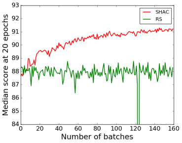
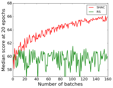
Figure 1: We compare the median function values of every batch of points proposed by RS and SHAC on CIFAR10 and CIFAR100 architecture search problems (see Section 4.3). Not surprisingly, the median score of the points proposed by RS fluctuates around a constant. As expected, the median scores of the points proposed by SHAC fluctuate around a monotonically increasing curve.

Binary classifiers: Within the SHAC algorithm, any family of binary classifiers can be used. In our experiments, we use gradient boosted trees [9] to classify points at every stages. Gradient boosted trees have shown to be flexible, fast (for both training and inference), robust to the choice to their own hyperparameters, and easy to get working in new problem domains [8]. These characteristics are all helpful properties of any black box optimization algorithm and accordingly we recommend using gradient boosted trees or random forests [24] within the SHAC algorithm. In all of our experiments, we use gradient boosted trees, fix the number of trees to be $200$ and do not change any of the other default hyperparameters in the XGBoost implementation [8]. It is expected that increasing the number of trees is likely to improve the performance at the cost of some computation overhead.

Maximum number of classifiers: If we train and adopt a classifier after every batch of points is evaluated, then we will end up with a maximum of $m-1$ classifiers. Given $K$ classifiers, to draw a new point that makes it past all of the classifiers, one needs to draw on average $2^{K}$ random points, one of which will be approved. In order to reduce the computational overhead, we limit the number of classifiers to a maximum of $18$ and define the number of classifiers as $K=\min(m-1,18)$.

Classifier budget: Given a budget of $N$ point evaluations and a total of $K$ classifiers, it is natural to distribute the budget evenly among the classifiers, so each classifier is trained on a reasonably sized dataset. To accomodate the parallel budget of $W$ workers, we set the minimum number of points per classifier to $T_{c}={W\lfloor\frac{N}{W(K+1)}\rfloor}$ in all our experiments. Further, to make sure that completely useless classifiers are not used, we only adopt a new classifier if its $5$-fold cross validation accuracy is at least $50\%$.

Algorithm 1 SHAC: Successive Halving and Classification

  Input: prior distribution $U(x)$, black-box objective $b(x)$, total budget $N$, classifier budget $T_{c}$

  Initialize: $C\leftarrow\{\}$

  Initialize: $S\leftarrow\{\}$

  for $t=1$ to $N$ do

     repeat

        Sample $x\sim U(x)$

     until $\forall c\in C:~{}c(x)>0$

     Evaluate $y=b(x)$

     $S\leftarrow S\cup\{(x,y)\}$

     if $|S|=T_{c}$ then

        $\{(x_{i},y_{i})\}_{i=1}^{\lvert S\rvert}\leftarrow S$

        $\tilde{y}=\operatorname{median}(\{y_{i}\}_{i=1}^{\lvert S\rvert})$

        $S^{\prime}=\{(x_{i},\mathrm{sign}(y_{i}-\tilde{y}))\}_{i=1}^{\lvert S\rvert}$

        Train a binary classifier $c$ on $S^{\prime}$

        $C\leftarrow C\cup\{c\}$

        $S\leftarrow\{\}$

     end if

  end for

4 Experiments

To assess the effectiveness of the SHAC algorithm, we compare SHAC with NAS-PPO: Neural Architecture Search [48] based on Proximal Policy Optimization (PPO) [35], RS: Random Search, and RS-2X: Random Search with twice the number of evaluations. We conduct experiments on architecture search and hyperparameter search on CIFAR-10 and CIFAR-100. We also run experiments on two synthetic test functions used by previous work: Branin and Hartmann6. The results for NAS are obtained with an implementation generously provided by the respective authors and we use the default configuration parameters of NAS. The NAS implementation is an improved version of [47] based on [35].

Since the entire search process, including the objective function, is highly stochastic, the top point found by each algorithm varies quite a bit across multiple runs. For architecture and hyperparameter search, it is computationally prohibitive to run the search multiple times, so we report the mean of the top $5$ values instead of the single best result.

4.1 Synthetic functions

We adopt the Branin and Hartmann6 synthetic functions used by prior work including [6]. These functions present accessible benchmarks that enable fast experimentation. For Hartmann6, $x$ is a continuous $6$D vector, and each dimension has a uniform prior in the interval $[0.0,1.0]$. For Branin, $x$ is a continuous $2$D vector, where the first and second dimensions have a uniform prior in the range of $[-5.0,10.0]$ and $[0.0,15.0]$ respectively. Since these functions are available in closed form, it is efficient to compute $b(x)$ at the proposed candidate points.

We compare SHAC to RS and RS-2X on a budget of $200$ and $400$ evaluations, where the budget is divided into batches of $20$ parallel evaluations. Each classifier in SHAC is trained on a dataset of $20$ points. Since $20$ points are not enough to obtain a reliable cross-validation estimate, we do not perform cross-validation here. We report the empirical results in Table 1. We note that the functions are being minimized here, so smaller numbers are preferred. Because these experiments are cheap, we run each method $5$ times using different random seeds and report the mean and standard error in Table 1. On both budgets on both functions, we observe that SHAC significantly outperforms RS-2X. For comparison, Spearmint [38], which uses a Gaussian Process for black box optimization achieves $0.398$ and $-3.133$ on Branin and Hartmann6 respectively using a sequence of $200$ function evaluations. Spearmint outperforms SHAC at at the cost of fully sequential evaluation, which is significantly slower in practice for real world applications. SHAC on the other hand, leverages $20$ parallel evaluations in each step, and unlike Gaussian Processes easily scales to very large datasets.

4.2 Hyperparameter Search

Dataset	(Batches, Workers)	RS	RS-2X	NAS-PPO	SHAC
Synthetic functions
Branin	20, 20	0.543 $\pm$ 0.06	0.457 $\pm$ 0.01	-	0.410 $\pm$ 0.01
Branin	20, 10	0.722 $\pm$ 0.1	0.543 $\pm$ 0.06	-	0.416 $\pm$ 0.01
Hartmann6	20, 20	-2.647 $\pm$ 0.13	-2.672 $\pm$ 0.07	-	-3.158 $\pm$ 0.04
Hartmann6	20, 10	-2.231 $\pm$ 0.04	-2.647 $\pm$ 0.13	-	-2.809 $\pm$ 0.04
Hyperparameter search at $100$ Epochs
CIFAR-10	16, 100	92.66	92.82	92.93	93.62
CIFAR-100	16, 100	69.23	69.23	69.82	71.66
Architecture search at $20$ Epochs
CIFAR-10	80, 100	91.72	91.83	92.72	92.54
CIFAR-100	80, 100	67.48	67.96	69.62	68.91

Table 1: We compare the performance of SHAC with RS, RS-2X, and NAS-PPO on optimizing architectures, hyperparameters and synthetic functions on varying budgets. For synthetic functions, we report the mean across $5$ trials and the standard error. For architecture and hyperparameter search, we report the mean of the top $5$ values at the end of the optimization procedure.

We cast hyperparameter search as black-box optimization, where the objective function is the validation accuracy of a network trained using a setting of hyperparameters. We fix the architecture to be NASNET-A [48] with $9$ cells and a greatly reduced filter size of $24$ for fast evaluation. We discretize the hyperparameters to be able to utilize the NAS-PPO code directly. A candidate point $x$ is a $20$D discrete vector that represents $20$ different hyperparameters including the learning rate, weight decay rate for each cell, label smoothing and the cell dropout rate for each cell. For the full specification of the search space, see the Appendix A.2. From the training sets of CIFAR-10 and CIFAR-100, we set aside validation sets with $5000$ examples. Each black-box evaluation $b(x)$ involves training NASNET-A for $100$ epochs on the training set and reporting the validation accuracy. We allow $1600$ evaluations for RS, NAS-PPO, and SHAC, with batches of $100$ workers. We set the maximum number of classifiers in SHAC to $15$ and the classifier budget to $100$ points per classifier.

We report the results in Table 1 and Figure 2. SHAC significantly outperforms RS-2X and NAS-PPO in these experiments. On CIFAR-10, SHAC obtains a $0.8\%$ gain over RS-2X and $0.69\%$ gain over NAS-PPO and on CIFAR-100, the gain over RS and NAS-PPO increases to $2.42\%$ and $1.84\%$ respectively. One may be able to achieve better results using NAS-PPO if they tune the hyperparameters of NAS-PPO itself, e.g., learning rate, entropy coefficient, etc. However, in real black box optimization, one does not have the luxury of tuning the optimization algorithm on different problems. To this end, we did not tune the hyperparameters of any of the algorithms and ran each algorithm once using the default parameters. SHAC achieves a significant improvement over random search without specific tuning for different search spaces and evaluation budgets.

4.3 Architecture Search

CIFAR-10	CIFAR-100

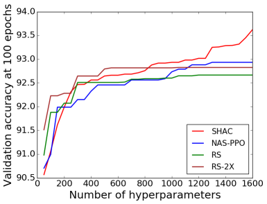
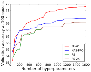
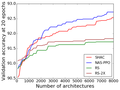
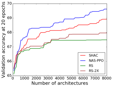
Figure 2: We plot the mean of the top-$5$ scores obtained by SHAC, NAS-PPO and RS on CIFAR-10 and CIFAR-100 on both hyperparameter and architecture search via $1600$ and $8000$ evaluations respectively.

We cast architecture search as black box optimization, where the objective function is the validation accuracy of a given architecture. For architecture search, a candidate point $x$ is a $40$D discrete code that represents the design choices for a convolutional cell. We follow the convolutional cell encoding proposed in [48] with minor modifications as communicated by the original authors as outlined in Appendix A.3. We use the same validation split as in the hyperparameter search experiments above. Each black box evaluation involves training an architecture defined by a $40$D code for $20$ epochs on the training set and reporting the validation accuracy. Each algorithm is provided with a budget of $8000$ total evaluations computed in parallel using $100$ workers. For SHAC this means the $8000$ evaluations are evenly split into $80$ synchronous rounds of $100$ evaluations. NAS is given an advantage by allowing the algorithm to update the RNN parameters every $5$ evaluations asynchronously. This is a more generous budget consistent with the conditions that NAS was designed for. For SHAC, we set the maximum number of classifiers to $18$ and the minimum budget per classifier to $400$.

We report the results in Table 1 and Figure 2. On CIFAR-10, SHAC demonstrates a gain of $0.8\%$ and $0.7\%$ over RS and RS-2X while underperforming NAS-PPO by $0.2\%$. On CIFAR-100, SHAC outperforms RS and RS-2X by $1.4\%$ and $0.9\%$ respectively, but underperforms NAS-PPO by $0.7\%$. We note that NAS-PPO is a complicated method with many hyperparameters that are fine-tuned for architecture search on this search space, whereas SHAC requires no tuning. Further, SHAC outperforms NAS-PPO on more realistic evaluation budgets discussed for hyperparameter search above. Finally, in what follows, we show that SHAC improves NAS-PPO in terms of architecture diversity, which leads to improved final accuracy when a shortlist of architectures is selected based on $20$ epochs and then trained for $300$ epochs.

4.4 Two-stage Architecture Search

To achieve the best results on CIFAR-10 and CIFAR-100, one needs to train relatively wide and deep neural nets for a few hundred epochs. Unfortunately, training deep architectures until convergence is extremely expensive making architecture search with thousands of point evaluations impractical. Previous work (e.g., [45] and [48]) suggests using a two-stage architecture search procedure, where one adopts a cheaper proxy objective to select a shortlist of top candidates. Then, the shortlist is evaluated on the real objective, and the best architectures are selected. During proxy evalution one trains a smaller shallower version of the architectures for a small number of epochs to improve training speed. We follow the proxy setup proposed by [48], where the architectures are trained for $20$ epochs first, as shown in Figure 2 and Table 1. Then, we select the top $50$ candidates based on the proxy evaluation and train a larger deeper version of such architectures for $300$ epochs, each $5$ times using different random seeds. We report the mean validation and test accuracy of the top $5$ architectures among the shortlist of $50$ for different algorithms in Table 2. Surprisingly, we find that all of the black box optimization algorithms are competitive in this regime, with SHAC and NAS achieving the best results on CIFAR-10 and CIFAR-100 respectively.

	Validation			Test
Dataset	RS	NAS-PPO	SHAC	RS	NAS-PPO	SHAC
CIFAR-10	96.11	96.16	96.30	95.67	95.87	95.91
CIFAR-100	79.06	79.53	79.37	79.59	79.93	79.80

Table 2: We select a shortlist of $50$ candidate architectures identified by each search algorithm based on their performance on the validation set after $20$ epochs. Then, we train each of these candidates for $300$ epochs and average their performance on the validation set across $5$ trials. We then report the mean performance of the top-$5$ architectures of each search algorithm on both the validation and test set, i.e., each number is an average across $25$ runs.

CIFAR-10	CIFAR-100

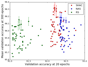
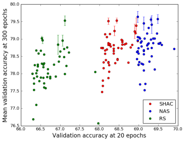
Figure 3: We plot the validation accuracy at $300$ epochs ("real" objective) averaged across 5 runs vs. $20$ epochs ("proxy" objective) for the top $50$ architectures found by each search algorithm. Error bars are shown for the top $5$ architectures based on the metric. We observe that there is a weak correlation between the proxy and final metric.

To investigate the correlation between the proxy and final objective functions we plot the final measurements as a function of the proxy evaluation in Figure 3 for the shortlist of top $50$ architectures selected by each algorithm. We find that the correlation between the proxy and the final metrics is not strong at least in this range of the proxy values. When there is a weak correlation between the proxy and the real objective, we advocate generating a diverse shortlist of candidates to avoid over-optimizing the proxy objective. Such a diversification strategy has been extensively studied in finance, where an investor constructs a diverse portfolio of investments by paying attention to both expectation of returns and variance of returns to mitigate unpredictable risks [29].

Random search naturally generates a diverse candidate shortlist. The cascade of $K$ classifiers in SHAC identifies a promising ${1}/{2^{K}}$th of the search space, which is still a large fraction of the original high dimensional space. SHAC exhibits no preference between the candidate points that make it past all of the classifiers, hence it tends to generate a diverse candidate shortlist for large search spaces. To study the shortlist diversity for different algorithms, we depict the histogram of the pairwise Hamming distances among the $40$D codes in the shortlist selected by each algorithm in Figure 4. We approximate the distance between two $40$D codes $x_{i}$ and $x_{j}$ representing two architectures via $\sum_{n=1}^{40}\mathbbm{1}(x_{i}^{n}\neq x_{j}^{n})$. This approximation gives us a general sense of the diversity in the population, but maybe improved using other metrics (e.g., [20]). In Figure 4, we observe that RS and SHAC have the most degree of diversity in the candidate shortlists followed by NAS-PPO, the mode of which is shifted to the left by $10$ units. Based on these results we conclude that given the SHAC algorithm presents consistent performance across differnt tasks and sample budgets (Table 1 and Table 2) despite its deceptively simple nature.

CIFAR-10	CIFAR-100

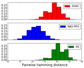
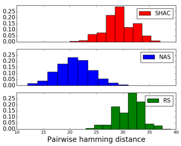
Figure 4: We plot a histogram of the pairwise hamming distances of the shortlist of $50$ architectures found by SHAC, NAS-PPO, and RS. RS and SHAC promote diversity in the candidates. We find this behavior consistent across both CIFAR-10 and CIFAR-100.

5 Conclusion

We propose a new algorithm for parallel black box optimization called SHAC that trains a cascade of binary classifiers to iteratively cull the undesirable regions of the search space. On hyperparameter search with moderate number of point evaluations, we significantly outperform NAS-PPO and RS-2X; random search with twice the number of evaluations. On architecture search, SHAC achieves competitive performance relative to NAS-PPO, while outperforming RS-2X. SHAC is simple to implement and requires no tuning of its own configuration parameters making it easy to use for practitioners and a baseline for further research in black-box optimization algorithms. Given the difficulty of benchmarking architecture search algorithms, one should have a strong bias towards algorithms like SHAC that are extremely simple to implement and apply.

6 Acknowledgements

We would like to thank Barret Zoph and Quoc Le for providing their implementation of the NAS-PPO and the convolutional cells used in [48]. Further, we would like to thank Azalia Mirhoseini, Barret Zoph, Carlos Riquelme, Ekin Dogus, Kevin Murphy, and Jonathen Shlens for their helpful suggestions and discussions at various phases of the project.

Appendix A Appendix

A.1 Hyperparameters for the convolutional networks

We train each architecture for $20$ epochs on the proxy objective using Adam optimizer [21], a learning rate of $0.01$, a weight decay of $10^{-4}$, a batch size of $256$, a filter size of $24$ and a cosine learning rate schedule. The validation accuracy at $20$ epochs is used as the proxy metric. We select a shortlist of $50$ architectures according to this proxy metric and train them with some hyperparameter changes to facilitate training longer and larger models. The filter size of the shortlisted architectures are increased to $64$ and then are trained for $300$ epochs using SGD with momentum, a learning rate of $0.1$, a smaller batch size of $64$, and a path dropout rate of $0.8$. For the shortlisted architectures we plot the mean validation accuracy at $300$ epochs across $5$ runs.

A.2 Search space for hyperparameter search

For hyperparameter search, we search over the learning rate, label smoothing, the dropout on the output activations of each of the 9 cells and the weight decay rate for each of the 9 cells thus obtaining a 20 dimensional search space. For each of these hyperparameters we search over the following possible values.

1. Label Smoothing - 0.0, 0.1, 0.2, 0.3, 0.4 and 0.5.

2. Learning rate - 0.0001, 0.00031623, 0.001, 0.01, 0.025, 0.04, 0.1, 0.31622777 and 1.

3. Weight decay rate - 1e-6, 1e-5, 5e-4, 1e-3, 1e-2 and 1e-1

4. Cell dropout - 0.0, 0.1, 0.2, 0.3, 0.4, 0.5, 0.6 and 0.7

A.3 Search Space for architecture search

For selecting architectures, we search over convolutional building blocks defined by Zoph et al. [48], with the following minor modifications based on the communications with the respective authors: (1) We remove the $5\!\times\!5$ and $7\!\times\!7$ max pooling operations. (2) We remove the option for choosing "the method for combining the hidden states" from the search space. By default, we combine the two hidden states by adding them. With these modifications, a cell is represented by a $40$ dimensional discrete code.

References

- Bahdanau et al. [2015] D. Bahdanau, K. Cho, and Y. Bengio. Neural machine translation by jointly learning to align and translate. ICLR, 2015.
- Baker et al. [2017a] B. Baker, O. Gupta, N. Naik, and R. Raskar. Designing neural network architectures using reinforcement learning. ICLR, 2017a.
- Baker et al. [2017b] B. Baker, O. Gupta, R. Raskar, and N. Naik. Accelerating neural architecture search using performance prediction. arXiv:1705.10823, 2017b.
- Bengio [2000] Y. Bengio. Gradient-based optimization of hyperparameters. Neural Computation, 2000.
- Bergstra and Bengio [2012] J. Bergstra and Y. Bengio. Random search for hyper-parameter optimization. JMLR, 2012.
- Bergstra et al. [2011] J. S. Bergstra, R. Bardenet, Y. Bengio, and B. Kégl. Algorithms for hyper-parameter optimization. NIPS, 2011.
- Brock et al. [2018] A. Brock, T. Lim, J. M. Ritchie, and N. Weston. Smash: one-shot model architecture search through hypernetworks. ICLR, 2018.
- Chen and Guestrin [2016] T. Chen and C. Guestrin. Xgboost: A scalable tree boosting system. KDD, 2016.
- Friedman [2001] J. H. Friedman. Greedy function approximation: a gradient boosting machine. Annals of statistics, 2001.
- Ha et al. [2016] D. Ha, A. Dai, and Q. V. Le. Hypernetworks. ICLR, 2016.
- Hashimoto et al. [2018] T. B. Hashimoto, S. Yadlowsky, and J. C. Duchi. Derivative free optimization via repeated classification. AISTATS, 2018.
- He et al. [2016] K. He, X. Zhang, S. Ren, and J. Sun. Deep residual learning for image recognition. CVPR, 2016.
- Hinton et al. [2012] G. Hinton, L. Deng, D. Yu, G. E. Dahl, A.-r. Mohamed, N. Jaitly, A. Senior, V. Vanhoucke, P. Nguyen, T. N. Sainath, et al. Deep neural networks for acoustic modeling in speech recognition: The shared views of four research groups. IEEE Signal Processing Magazine, 2012.
- Holland [1992] J. H. Holland. Adaptation in natural and artificial systems: an introductory analysis with applications to biology, control, and artificial intelligence. MIT press, 1992.
- Huang et al. [2017] G. Huang, Z. Liu, K. Q. Weinberger, and L. van der Maaten. Densely connected convolutional networks. CVPR, 2017.
- Hutter et al. [2011] F. Hutter, H. H. Hoos, and K. Leyton-Brown. Sequential model-based optimization for general algorithm configuration. International Conference on Learning and Intelligent Optimization, 2011.
- Ioffe and Szegedy [2015] S. Ioffe and C. Szegedy. Batch normalization: Accelerating deep network training by reducing internal covariate shift. ICML, 2015.
- Jaderberg et al. [2017] M. Jaderberg, V. Dalibard, S. Osindero, W. M. Czarnecki, J. Donahue, A. Razavi, O. Vinyals, T. Green, I. Dunning, K. Simonyan, et al. Population based training of neural networks. arXiv:1711.09846, 2017.
- Jamieson and Talwalkar [2016] K. Jamieson and A. Talwalkar. Non-stochastic best arm identification and hyperparameter optimization. AISTATS, 2016.
- Kandasamy et al. [2018] K. Kandasamy, W. Neiswanger, J. Schneider, B. Poczos, and E. Xing. Neural architecture search with bayesian optimisation and optimal transport. arXiv:1802.07191, 2018.
- Kingma and Ba [2014] D. P. Kingma and J. Ba. Adam: A method for stochastic optimization. arXiv:1412.6980, 2014.
- Krizhevsky et al. [2012] A. Krizhevsky, I. Sutskever, and G. E. Hinton. Imagenet classification with deep convolutional neural networks. NIPS, 2012.
- Li et al. [2016] L. Li, K. Jamieson, G. DeSalvo, A. Rostamizadeh, and A. Talwalkar. Hyperband: A novel bandit-based approach to hyperparameter optimization. arXiv:1603.06560, 2016.
- Liaw et al. [2002] A. Liaw, M. Wiener, et al. Classification and regression by randomforest. R news, 2(3):18–22, 2002.
- Liu et al. [2017a] C. Liu, B. Zoph, J. Shlens, W. Hua, L.-J. Li, L. Fei-Fei, A. Yuille, J. Huang, and K. Murphy. Progressive neural architecture search. arXiv:1712.00559, 2017a.
- Liu et al. [2017b] C. Liu, B. Zoph, J. Shlens, W. Hua, L.-J. Li, L. Fei-Fei, A. Yuille, J. Huang, and K. Murphy. Progressive neural architecture search. arXiv:1712.00559, 2017b.
- Liu et al. [2018] H. Liu, K. Simonyan, O. Vinyals, C. Fernando, and K. Kavukcuoglu. Hierarchical representations for efficient architecture search. ICLR, 2018.
- Maclaurin et al. [2015] D. Maclaurin, D. Duvenaud, and R. Adams. Gradient-based hyperparameter optimization through reversible learning. ICML, 2015.
- Markowitz [1952] H. Markowitz. Portfolio selection. The journal of finance, 1952.
- Miikkulainen et al. [2017] R. Miikkulainen, J. Liang, E. Meyerson, A. Rawal, D. Fink, O. Francon, B. Raju, A. Navruzyan, N. Duffy, and B. Hodjat. Evolving deep neural networks. arXiv:1703.00548, 2017.
- Miller et al. [1989] G. F. Miller, P. M. Todd, and S. U. Hegde. Designing neural networks using genetic algorithms. ICGA, 1989.
- Negrinho and Gordon [2017] R. Negrinho and G. Gordon. Deeparchitect: Automatically designing and training deep architectures. arXiv:1704.08792, 2017.
- Nesterov [2013] Y. Nesterov. Introductory lectures on convex optimization: A basic course. Springer Science & Business Media, 2013.
- Real et al. [2017] E. Real, S. Moore, A. Selle, S. Saxena, Y. L. Suematsu, Q. Le, and A. Kurakin. Large-scale evolution of image classifiers. ICML, 2017.
- Schulman et al. [2017] J. Schulman, F. Wolski, P. Dhariwal, A. Radford, and O. Klimov. Proximal policy optimization algorithms. arXiv:1707.06347, 2017.
- Simonyan and Zisserman [2015] K. Simonyan and A. Zisserman. Very deep convolutional networks for large-scale image recognition. ICLR, 2015.
- Snoek et al. [2012] J. Snoek, H. Larochelle, and R. P. Adams. Practical bayesian optimization of machine learning algorithms. NIPS, 2012.
- Snoek et al. [2014] J. Snoek, K. Swersky, R. Zemel, and R. Adams. Input warping for bayesian optimization of non-stationary functions. International Conference on Machine Learning, pages 1674–1682, 2014.
- Snoek et al. [2015] J. Snoek, O. Rippel, K. Swersky, R. Kiros, N. Satish, N. Sundaram, M. Patwary, M. Prabhat, and R. Adams. Scalable bayesian optimization using deep neural networks. ICML, 2015.
- Srivastava et al. [2014] N. Srivastava, G. Hinton, A. Krizhevsky, I. Sutskever, and R. Salakhutdinov. Dropout: A simple way to prevent neural networks from overfitting. JMLR, 2014.
- Stanley and Miikkulainen [2002] K. O. Stanley and R. Miikkulainen. Evolving neural networks through augmenting topologies. Evolutionary computation, 2002.
- Sutton and Barto [1998] R. S. Sutton and A. G. Barto. Introduction to Reinforcement Learning. MIT Press, 1998.
- Szegedy et al. [2015] C. Szegedy, W. Liu, Y. Jia, P. Sermanet, S. Reed, D. Anguelov, D. Erhan, V. Vanhoucke, A. Rabinovich, et al. Going deeper with convolutions. CVPR, 2015.
- Vaswani et al. [2017] A. Vaswani, N. Shazeer, N. Parmar, J. Uszkoreit, L. Jones, A. N. Gomez, L. Kaiser, and I. Polosukhin. Attention is all you need. NIPS, 2017.
- Xie and Yuille [2017] L. Xie and A. Yuille. Genetic cnn. ICCV, 2017.
- Zhong et al. [2018] Z. Zhong, J. Yan, and C.-L. Liu. Practical network blocks design with q-learning. AAAI, 2018.
- Zoph and Le [2017] B. Zoph and Q. V. Le. Neural architecture search with reinforcement learning. ICLR, 2017.
- Zoph et al. [2017] B. Zoph, V. Vasudevan, J. Shlens, and Q. V. Le. Learning transferable architectures for scalable image recognition. arXiv:1707.07012, 2017.