How Much Restricted Isometry is Needed In Nonconvex Matrix Recovery?††thanks: 32nd Conference on Neural Information Processing Systems (NIPS 2018), Montréal, Canada.
Abstract
When the linear measurements of an instance of low-rank matrix recovery satisfy a restricted isometry property (RIP)—i.e. they are approximately norm-preserving—the problem is known to contain no spurious local minima, so exact recovery is guaranteed. In this paper, we show that moderate RIP is not enough to eliminate spurious local minima, so existing results can only hold for near-perfect RIP. In fact, counterexamples are ubiquitous: we prove that every is the spurious local minimum of a rank-1 instance of matrix recovery that satisfies RIP. One specific counterexample has RIP constant , but causes randomly initialized stochastic gradient descent (SGD) to fail 12% of the time. SGD is frequently able to avoid and escape spurious local minima, but this empirical result shows that it can occasionally be defeated by their existence. Hence, while exact recovery guarantees will likely require a proof of no spurious local minima, arguments based solely on norm preservation will only be applicable to a narrow set of nearly-isotropic instances.
1 Introduction
Recently, several important nonconvex problems in machine learning have been shown to contain no spurious local minima [19, 4, 21, 8, 20, 34, 30]. These problems are easily solved using local search algorithms despite their nonconvexity, because every local minimum is also a global minimum, and every saddle-point has sufficiently negative curvature to allow escape. Formally, the usual first- and second-order necessary conditions for local optimality (i.e. zero gradient and a positive semidefinite Hessian) are also sufficient for global optimality; satisfying them to -accuracy will yield a point within an -neighborhood of a globally optimal solution.
Many of the best-understood nonconvex problems with no spurious local minima are variants of the low-rank matrix recovery problem. The simplest version (known as matrix sensing) seeks to recover an positive semidefinite matrix of low rank , given measurement matrices and noiseless data . The usual, nonconvex approach is to solve the following
| (1) |
to second-order optimality, using a local search algorithm like (stochastic) gradient descent [19, 24] and trust region Newton’s method [16, 7], starting from a random initial point.
Exact recovery of the ground truth is guaranteed under the assumption that satisfies the restricted isometry property [14, 13, 31, 11] with a sufficiently small constant. The original result is due to Bhojanapalli et al. [4], though we adapt the statement below from a later result by Ge et al. [20, Theorem 8]. (Zhu et al. [43] give an equivalent statement for nonsymmetric matrices.)
Definition 1 (Restricted Isometry Property).
The linear map is said to satisfy -RIP with constant if there exists a fixed scaling such that for all rank- matrices :
| (2) |
We say that satisfies -RIP if satisfies -RIP with some .
Theorem 2 (No spurious local minima).
Let satisfy -RIP with . Then, (1) has no spurious local minima: every local minimum satisfies , and every saddle point has an escape (the Hessian has a negative eigenvalue). Hence, any algorithm that converges to a second-order critical point is guaranteed to recover exactly.
Standard proofs of Theorem 2 use a norm-preserving argument: if satisfies -RIP with a small constant , then we can view the least-squares residual as a dimension-reduced embedding of the displacement vector , as in
| (3) |
The high-dimensional problem of minimizing over contains no spurious local minima, so its dimension-reduced embedding (1) should satisfy a similar statement. Indeed, this same argument can be repeated for noisy measurements and nonsymmetric matrices to result in similar guarantees [4, 20].
The norm-preserving argument also extends to “harder” choices of that do not satisfy RIP over its entire domain. In the matrix completion problem, the RIP-like condition holds only when is both low-rank and sufficiently dense [12]. Nevertheless, Ge et al. [21] proved a similar result to Theorem 2 for this problem, by adding a regularizing term to the objective. For a detailed introduction to the norm-preserving argument and its extension with regularizers, we refer the interested reader to [21, 20].
1.1 How much restricted isometry?
The RIP threshold in Theorem 2 is highly conservative—it is only applicable to nearly-isotropic measurements like Gaussian measurements. Let us put this point into perspective by measuring distortion using the condition number111Given a linear map, the condition number measures the ratio in size between the largest and smallest images, given a unit-sized input. Within our specific context, the -restricted condition number is the smallest such that holds for all rank- matrices . . Deterministic linear maps from real-life applications usually have condition numbers between and , and these translate to RIP constants between and . By contrast, the RIP threshold requires an equivalent condition number of , which would be considered near-perfect in linear algebra.
In practice, nonconvex matrix completion works for a much wider class of problems than those suggested by Theorem 2 [6, 5, 32, 1]. Indeed, assuming only that satisfies -RIP, solving (1) to global optimality is enough to guarantee exact recovery [31, Theorem 3.2]. In turn, stochastic algorithms like stochastic gradient descent (SGD) are often able to attain global optimality. This disconnect between theory and practice motivates the following question.
Can Theorem 2 be substantially improved—is it possible to guarantee the inexistence of spurious local minima with -RIP and any value of ?
At a basic level, the question gauges the generality and usefulness of RIP as a base assumption for nonconvex recovery. Every family of measure operators —even correlated and “bad” measurement ensembles—will eventually come to satisfy -RIP as the number of measurements grows large. Indeed, given linearly independent measurements, the operator becomes invertible, and hence trivially -RIP. In this limit, recovering the ground truth from noiseless measurements is as easy as solving a system of linear equations. Yet, it remains unclear whether nonconvex recovery is guaranteed to succeed.
At a higher level, the question also gauges the wisdom of exact recovery guarantees through “no spurious local minima”. It may be sufficient but not necessary; exact recovery may actually hinge on SGD’s ability to avoid and escape spurious local minima when they do exist. Indeed, there is growing empirical evidence that SGD outmaneuvers the “optimization landscape” of nonconvex functions [6, 5, 27, 32, 1], and achieves some global properties [22, 40, 39]. It remains unclear whether the success of SGD for matrix recovery should be attributed to the inexistence of spurious local minima, or to some global property of SGD.
1.2 Our results
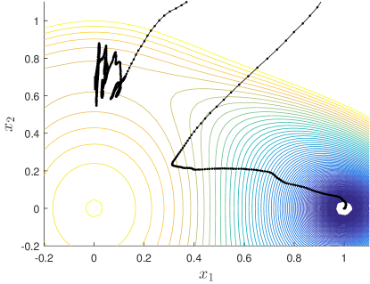
In this paper, we give a strong negative answer to the question above. Consider the counterexample below, which satisfies -RIP with , but nevertheless contains a spurious local minimum that causes SGD to fail in 12% of trials.
Example 3.
Consider the following -RIP instance of (1) with matrices
Note that the associated operator is invertible and satisfies for all . Nevertheless, the point satisfies second-order optimality,
and randomly initialized SGD can indeed become stranded around this point, as shown in Figure 1. Repeating these trials 100,000 times yields 87,947 successful trials, for a failure rate of to three standard deviations.

Accordingly, RIP-based exact recovery guarantees like Theorem 2 cannot be improved beyond . Otherwise, spurious local minima can exist, and SGD may become trapped. Using a local search algorithm with a random initialization, “no spurious local minima” is not only sufficient for exact recovery, but also necessary.
In fact, there exists an infinite number of counterexamples like Example 3. In Section 3, we prove that, in the rank-1 case, almost every choice of generates an instance of (1) with a strict spurious local minimum.
Theorem 4 (Informal).
Let be nonzero and not colinear. Then, there exists an instance of (1) satisfying -RIP with that has as the ground truth and as a strict spurious local minimum, i.e. with zero gradient and a positive definite Hessian. Moreover, is bounded in terms of the length ratio and the incidence angle satisfying as
It is therefore impossible to establish “no spurious local minima” guarantees unless the RIP constant is small. This is a strong negative result on the generality and usefulness of RIP as a base assumption, and also on the wider norm-preserving argument described earlier in the introduction. In Section 4, we provide strong empirical evidence for the following sharp version of Theorem 2.
Conjecture 5.
How is the practical performance of SGD affected by spurious local minima? In Section 5, we apply randomly initialized SGD to instances of (1) engineered to contain spurious local minima. In one case, SGD recovers the ground truth with a 100% success rate, as if the spurious local minima did not exist. But in another case, SGD fails in 59 of 1,000 trials, for a positive failure rate of to three standard deviations. Examining the failure cases, we observe that SGD indeed becomes trapped around a spurious local minimum, similar to Figure 1 in Example 3.
1.3 Related work
There have been considerable recent interest in understanding the empirical “hardness” of nonconvex optimization, in view of its well-established theoretical difficulties. Nonconvex functions contain saddle points and spurious local minima, and local search algorithms may become trapped in them. Recent work have generally found the matrix sensing problem to be “easy”, particularly under an RIP-like incoherence assumption. Our results in this paper counters this intuition, showing—perhaps surprisingly—that the problem is generically “hard” even under RIP.
Comparison to convex recovery. Classical theory for the low-rank matrix recovery problem is based on convex relaxation: replacing in (1) by a convex term , and augmenting the objective with a trace penalty to induce a low-rank solution [12, 31, 15, 11]. The convex approach enjoys RIP-based exact recovery guarantees [11], but these are also fundamentally restricted to small RIP constants [10, 38]—in direct analogy with our results for nonconvex recovery. In practice, convex recovery is usually much more expensive than nonconvex recovery, because it requires optimizing over an matrix variable instead of an vector-like variable. On the other hand, it is statistically consistent [3], and guaranteed to succeed with noiseless, linearly independent measurements. By comparison, our results show that nonconvex recovery can still fail in this regime.
Convergence to spurious local minima. Recent results on “no spurious local minima” are often established using a norm-preserving argument: the problem at hand is the low-dimension embedding of a canonical problem known to contain no spurious local minima [19, 34, 35, 4, 21, 20, 30, 43]. While the approach is widely applicable in its scope, our results in this paper finds it to be restrictive in the problem data. More specifically, the measurement matrices must come from a nearly-isotropic ensemble like the Gaussian and the sparse binary.
Special initialization schemes. An alternative way to guarantee exact recovery is to place the initial point sufficiently close to the global optimum [25, 26, 23, 42, 41, 36]. This approach is more general because it does not require a global “no spurious local minima” guarantee. On the other hand, good initializations are highly problem-specific and difficult to generalize. Our results show that spurious local minima can exist arbitrarily close to the solution. Hence, exact recovery guarantees must give proof of local attraction, beyond simply starting close to the ground truth.
Ability of SGD to escape spurious local minima. Practitioners have long known that stochastic gradient descent (SGD) enjoys properties inherently suitable for the sort of nonconvex optimization problems that appear in machine learning [27, 6], and that it is well-suited for generalizing unseen data [22, 40, 39]. Its specific behavior is yet not well understood, but it is commonly conjectured that SGD outperforms classically “better” algorithms like BFGS because it is able to avoid and escape spurious local minima. Our empirical findings in Section 5 partially confirms this suspicion, showing that randomly initialized SGD is sometimes able to avoid and escape spurious local minima as if they did not exist. In other cases, however, SGD can indeed become stuck at a local minimum, thereby resulting in a positive failure rate.
Notation
We use to refer to any candidate point, and to refer to a rank- factorization of the ground truth . For clarity, we use lower-case even when these are matrices.
The sets are the space of real matrices and real symmetric matrices, and and are the Frobenius inner product and norm. We write (resp. ) if is positive semidefinite (resp. positive definite). Given a matrix , its spectral norm is , and its eigenvalues are . If , then and , . If is invertible, then its condition number is ; if not, then .
The vectorization operator preserves inner products and Euclidean norms . In each case, the matricization operator is the inverse of .
2 Key idea: Spurious local minima via convex optimization
Given arbitrary and rank- positive semidefinite matrix , consider the problem of finding an instance of (1) with as the ground truth and as a spurious local minimum. While not entirely obvious, this problem is actually convex, because the first- and second-order optimality conditions associated with (1) are linear matrix inequality (LMI) constraints [9] with respect to the kernel operator . The problem of finding an instance of (1) that also satisfies RIP is indeed nonconvex. However, we can use the condition number of as a surrogate for the RIP constant of : if the former is finite, then the latter is guaranteed to be less than 1. The resulting optimization is convex, and can be numerically solved using an interior-point method, like those implemented in SeDuMi [33], SDPT3 [37], and MOSEK [2], to high accuracy.
We begin by fixing some definitions. Given a choice of and the ground truth , we define the nonconvex objective
| (4) |
whose value is always nonnegative by construction. If the point attains , then we call it a global minimum; otherwise, we call it a spurious point. Under RIP, is a global minimum if and only if [31, Theorem 3.2]. The point is said to be a local minimum if holds for all within a local neighborhood of . If is a local minimum, then it must satisfy the first and second-order necessary optimality conditions (with some fixed ):
| (5) | ||||||
| (6) |
Conversely, if satisfies the second-order sufficient optimality conditions, that is (5)-(6) with , then it is a local minimum. Local search algorithms are only guaranteed to converge to a first-order critical point satisfying (5), or a second-order critical point satisfying (5)-(6) with . The latter class of algorithms include stochastic gradient descent [19], randomized and noisy gradient descent [19, 28, 24, 18], and various trust-region methods [17, 29, 16, 7].
Given arbitrary choices of , we formulate the problem of picking an satisfying (5) and (6) as an LMI feasibility. First, we define satisfying for all as the matrix representation of the operator . Then, we rewrite (5) and (6) as and , where the linear operators and are defined
| (7) | |||||
| (8) |
with respect to the error vector and the matrix that implements the symmetric product operator . To compute a choice of satisfying and , we solve the following LMI feasibility problem
| (9) |
and factor a feasible back into , e.g. using Cholesky factorization or an eigendecomposition. Once a matrix representation is found, we recover the matrices implementing the operator by matricizing each row of .
Now, the problem of picking with the smallest condition number may be formulated as the following LMI optimization
| (10) |
with solution . Then, is the best condition number achievable, and any recovered from will satisfy
for all , that is, with any rank. As such, is -RIP with , and hence also -RIP with for all ; see e.g. [31, 11]. If the optimal value is strictly positive, then the recovered yields an RIP instance of (1) with as the ground truth and as a spurious local minimum, as desired.
It is worth emphasizing that a small condition number—a large in (10)—will always yield a small RIP constant , which then bounds all other RIP constants via for all . However, the converse direction is far less useful, as the value of does not preclude with from being small.
3 Closed-form solutions
It turns out that the LMI problem (10) in the rank-1 case is sufficiently simple that it can be solved in closed-form. (All proofs are given in the Appendix.) Let be arbitrary nonzero vectors, and define
| (11) |
as their associated length ratio and incidence angle. We begin by examining the prevalence of spurious critical points.
Theorem 6 (First-order optimality).
The point is always a local maximum for , and hence a spurious first-order critical point. With a perfect RIP constant , Theorem 6 says that is also the only spurious first-order critical point. Otherwise, spurious first-order critical points may exist elsewhere, even when the RIP constant is arbitrarily close to zero. This result highlights the importance of converging to second-order optimality, in order to avoid getting stuck at a spurious first-order critical point.
Next, we examine the prevalence of spurious local minima.
Theorem 7 (Second-order optimality).
If and , then is guaranteed to be a strict local minimum for a problem instance satisfying -RIP. Hence, we must conclude that spurious local minima are ubiquitous. The associated RIP constant is not too much worse than than the figure quoted in Theorem 6. On the other hand, spurious local minima must cease to exist once according to Theorem 2.
4 Experiment 1: Minimum with spurious local minima
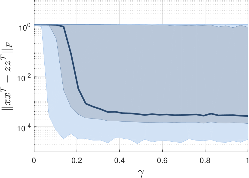
What is smallest RIP constant that still admits an instance of (1) with spurious local minima? Let us define the threshold value as the following
| (13) |
Here, we write , and optimize over the spurious local minimum the rank- ground truth , and the linear operator . Note that gives a “no spurious local minima” guarantee, due to the inexistence of counterexamples.
Proposition 8.
Let satisfy -RIP. If , then (1) has no spurious local minimum.
Proof.
Our convex formulation in Section 2 bounds from above. Specifically, our LMI problem (10) with optimal value is equivalent to the following variant of (13)
| (14) |
with optimal value . Now, (14) gives an upper-bound on (13) because -RIP is a sufficient condition for -RIP. Hence, we have for every valid choice of and .
The same convex formulation can be modified to bound from below222We thank an anonymous reviewer for this key insight.. Specifically, a necessary condition for to satisfy -RIP is the following
| (15) |
where is a fixed matrix. This is a convex linear matrix inequality; substituting (15) into (13) in lieu of of -RIP yields a convex optimization problem
| (16) |
that generates lower-bounds .
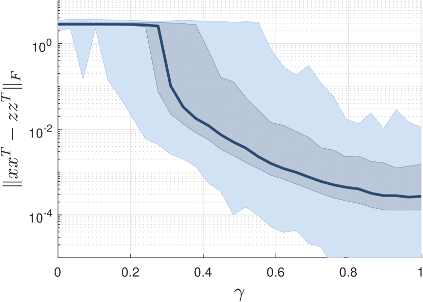
Our best upper-bound is likely . The existence of Example 3 gives the upper-bound of . To improve upon this bound, we randomly sample i.i.d. from the standard Gaussian, and evaluate using MOSEK [2]. We perform the experiment for 3 hours on each tuple but obtain for every and considered.
The threshold is likely . Now, we randomly sample i.i.d. from the standard Gaussian. For each fixed , we set and evaluate using MOSEK [2]. We perform the same experiment as the above, but find that for every and considered. Combined with the existence of the upper-bound , these experiments strongly suggest that .
5 Experiment 2: SGD escapes spurious local minima
How is the performance of SGD affected by the presence of spurious local minima? Given that spurious local minima cease to exist with , we might conjecture that the performance of SGD is a decreasing function of . Indeed, this conjecture is generally supported by evidence from the nearly-isotropic measurement ensembles [6, 5, 32, 1], all of which show improving performance with increasing number of measurements .
This section empirically measures SGD (with momentum, fixed learning rates, and batchsizes of one) on two instances of (1) with different values of , both engineered to contain spurious local minima by numerically solving (10). We consider a “bad” instance, with and rank , and a “good” instance, with and rank . The condition number of the “bad” instance is 25 times higher than the “good” instance, so classical theory suggests the former to be a factor of 5-25 times harder to solve than the former. Moreover, the “good” instance is locally strongly convex at its isolated global minima while the “bad” instance is only locally weakly convex, so first-order methods like SGD should locally converge at a linear rate for the former, and sublinearly for the latter.
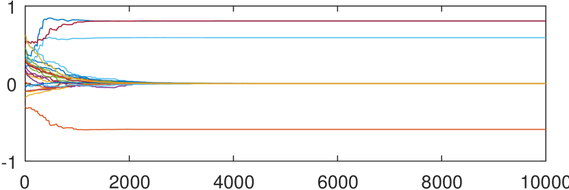
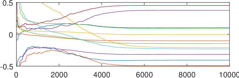
SGD consistently succeeds on “bad” instance with and . We generate the “bad” instance by fixing , , selecting i.i.d. from the standard Gaussian, rescale so that and rescale so that , and solving (10); the results are shown in Figure 3. The results at validate as a true local minimum: if initialized here, then SGD remains stuck here with error. The results at shows randomly initialized SGD either escaping our engineered spurious local minimum, or avoiding it altogether. All 1,000 trials at recover the ground truth to accuracy, with 95% quantile at .
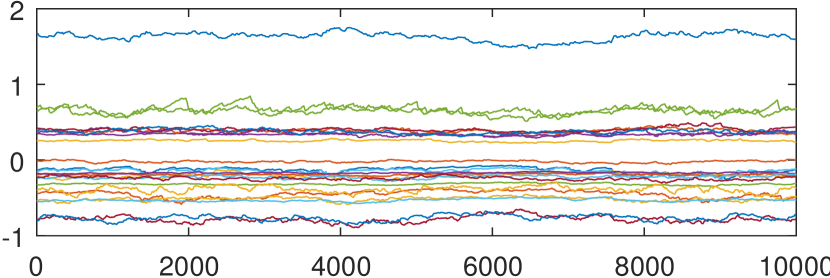
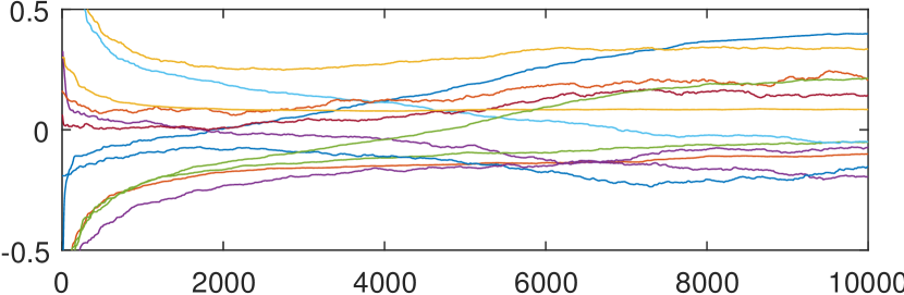
SGD consistently fails on “good” instance with and . We generate the “good” instance with and using the procedure in the previous Section; the results are shown in Figure 3. As expected, the results at validate as a true local minimum. However, even with yielding a random initialization, 59 of the 1,000 trials still result in an error of , thereby yielding a failure rate of up to three standard deviations. Examine the failed trials closer, we do indeed find SGD hovering around our engineered spurious local minimum.
Repeating the experiment over other instances of (1) obtained by solving (10) with randomly selected , we generally obtain graphs that look like Figure 3. In other words, SGD usually escapes spurious local minima even when they are engineered to exist. These observations continue to hold true with even massive condition numbers on the order of , with corresponding RIP constant . On the other hand, we do occasionally sample well-conditioned instances that behave closer to the “good” instance describe above, causing SGD to consistently fail.
6 Conclusions
The nonconvex formulation of low-rank matrix recovery is highly effective, despite the apparent risk of getting stuck at a spurious local minimum. Recent results have shown that if the linear measurements of the low-rank matrix satisfy a restricted isometry property (RIP), then the problem contains no spurious local minima, so exact recovery is guaranteed. Most of these existing results are based on a norm-preserving argument: relating and arguing that a lack of spurious local minima in the latter implies a similar statement in the former.
Our key message in this paper is that moderate RIP is not enough to eliminate spurious local minima. To prove this, we formulate a convex optimization problem in Section 2 that generates counterexamples that satisfy RIP but contain spurious local minima. Solving this convex formulation in closed-form in Section 3 shows that counterexamples are ubiquitous: almost any rank-1 and any can respectively be the ground truth and spurious local minimum to an instance of matrix recovery satisfying RIP. We gave one specific counterexample with RIP constant in the introduction that causes randomly initialized stochastic gradient descent (SGD) to fail 12% of the time.
Moreover, stochastic gradient descent (SGD) is often but not always able to avoid and escape spurious local minima. In Section 5, randomly initialized SGD solved one example with a 100% success rate over 1,000 trials, despite the presence of spurious local minima. However, it failed with a consistent rate of on another other example with an RIP constant of just . Hence, as long as spurious local minima exist, we cannot expect to guarantee exact recovery with SGD (without a much deeper understanding of the algorithm).
Overall, exact recovery guarantees will generally require a proof of no spurious local minima. However, arguments based solely on norm preservation are conservative, because most measurements are not isotropic enough to eliminate spurious local minima.
Acknowledgements
We thank our three NIPS reviewers for helpful comments and suggestions. In particular, we thank reviewer #2 for a key insight that allowed us to lower-bound in Section 4. This work was supported by the ONR Awards N00014-17-1-2933 and ONR N00014-18-1-2526, NSF Award 1808859, DARPA Award D16AP00002, and AFOSR Award FA9550- 17-1-0163.
References
- [1] Alekh Agarwal, Olivier Chapelle, Miroslav Dudík, and John Langford. A reliable effective terascale linear learning system. The Journal of Machine Learning Research, 15(1):1111–1133, 2014.
- [2] Erling D Andersen and Knud D Andersen. The MOSEK interior point optimizer for linear programming: an implementation of the homogeneous algorithm. In High performance optimization, pages 197–232. Springer, 2000.
- [3] Francis R Bach. Consistency of trace norm minimization. Journal of Machine Learning Research, 9(Jun):1019–1048, 2008.
- [4] Srinadh Bhojanapalli, Behnam Neyshabur, and Nati Srebro. Global optimality of local search for low rank matrix recovery. In Advances in Neural Information Processing Systems, pages 3873–3881, 2016.
- [5] Léon Bottou. Large-scale machine learning with stochastic gradient descent. In Proceedings of COMPSTAT’2010, pages 177–186. Springer, 2010.
- [6] Léon Bottou and Olivier Bousquet. The tradeoffs of large scale learning. In Advances in neural information processing systems, pages 161–168, 2008.
- [7] Nicolas Boumal, P-A Absil, and Coralia Cartis. Global rates of convergence for nonconvex optimization on manifolds. IMA Journal of Numerical Analysis, 2018.
- [8] Nicolas Boumal, Vlad Voroninski, and Afonso Bandeira. The non-convex Burer-Monteiro approach works on smooth semidefinite programs. In Advances in Neural Information Processing Systems, pages 2757–2765, 2016.
- [9] Stephen Boyd, Laurent El Ghaoui, Eric Feron, and Venkataramanan Balakrishnan. Linear matrix inequalities in system and control theory, volume 15. SIAM, 1994.
- [10] T Tony Cai and Anru Zhang. Sharp RIP bound for sparse signal and low-rank matrix recovery. Applied and Computational Harmonic Analysis, 35(1):74–93, 2013.
- [11] Emmanuel J Candes and Yaniv Plan. Tight oracle inequalities for low-rank matrix recovery from a minimal number of noisy random measurements. IEEE Transactions on Information Theory, 57(4):2342–2359, 2011.
- [12] Emmanuel J Candès and Benjamin Recht. Exact matrix completion via convex optimization. Foundations of Computational mathematics, 9(6):717, 2009.
- [13] Emmanuel J Candes, Justin K Romberg, and Terence Tao. Stable signal recovery from incomplete and inaccurate measurements. Communications on pure and applied mathematics, 59(8):1207–1223, 2006.
- [14] Emmanuel J Candes and Terence Tao. Decoding by linear programming. IEEE transactions on information theory, 51(12):4203–4215, 2005.
- [15] Emmanuel J Candès and Terence Tao. The power of convex relaxation: Near-optimal matrix completion. IEEE Transactions on Information Theory, 56(5):2053–2080, 2010.
- [16] Coralia Cartis, Nicholas IM Gould, and Ph L Toint. Complexity bounds for second-order optimality in unconstrained optimization. Journal of Complexity, 28(1):93–108, 2012.
- [17] Andrew R Conn, Nicholas IM Gould, and Ph L Toint. Trust region methods, volume 1. SIAM, 2000.
- [18] Simon S Du, Chi Jin, Jason D Lee, Michael I Jordan, Aarti Singh, and Barnabas Poczos. Gradient descent can take exponential time to escape saddle points. In Advances in Neural Information Processing Systems, pages 1067–1077, 2017.
- [19] Rong Ge, Furong Huang, Chi Jin, and Yang Yuan. Escaping from saddle points–online stochastic gradient for tensor decomposition. In Conference on Learning Theory, pages 797–842, 2015.
- [20] Rong Ge, Chi Jin, and Yi Zheng. No spurious local minima in nonconvex low rank problems: A unified geometric analysis. In International Conference on Machine Learning, pages 1233–1242, 2017.
- [21] Rong Ge, Jason D Lee, and Tengyu Ma. Matrix completion has no spurious local minimum. In Advances in Neural Information Processing Systems, pages 2973–2981, 2016.
- [22] Moritz Hardt, Ben Recht, and Yoram Singer. Train faster, generalize better: Stability of stochastic gradient descent. In International Conference on Machine Learning, pages 1225–1234, 2016.
- [23] Prateek Jain, Praneeth Netrapalli, and Sujay Sanghavi. Low-rank matrix completion using alternating minimization. In Proceedings of the forty-fifth annual ACM symposium on Theory of computing, pages 665–674. ACM, 2013.
- [24] Chi Jin, Rong Ge, Praneeth Netrapalli, Sham M Kakade, and Michael I Jordan. How to escape saddle points efficiently. In International Conference on Machine Learning, pages 1724–1732, 2017.
- [25] Raghunandan H Keshavan, Andrea Montanari, and Sewoong Oh. Matrix completion from a few entries. IEEE Transactions on Information Theory, 56(6):2980–2998, 2010.
- [26] Raghunandan H Keshavan, Andrea Montanari, and Sewoong Oh. Matrix completion from noisy entries. Journal of Machine Learning Research, 11(Jul):2057–2078, 2010.
- [27] Alex Krizhevsky, Ilya Sutskever, and Geoffrey E Hinton. Imagenet classification with deep convolutional neural networks. In Advances in neural information processing systems, pages 1097–1105, 2012.
- [28] Jason D Lee, Max Simchowitz, Michael I Jordan, and Benjamin Recht. Gradient descent only converges to minimizers. In Conference on Learning Theory, pages 1246–1257, 2016.
- [29] Yurii Nesterov and Boris T Polyak. Cubic regularization of newton method and its global performance. Mathematical Programming, 108(1):177–205, 2006.
- [30] Dohyung Park, Anastasios Kyrillidis, Constantine Carmanis, and Sujay Sanghavi. Non-square matrix sensing without spurious local minima via the Burer-Monteiro approach. In Artificial Intelligence and Statistics, pages 65–74, 2017.
- [31] Benjamin Recht, Maryam Fazel, and Pablo A Parrilo. Guaranteed minimum-rank solutions of linear matrix equations via nuclear norm minimization. SIAM Review, 52(3):471–501, 2010.
- [32] Benjamin Recht and Christopher Ré. Parallel stochastic gradient algorithms for large-scale matrix completion. Mathematical Programming Computation, 5(2):201–226, 2013.
- [33] Jos F Sturm. Using SeDuMi 1.02, a MATLAB toolbox for optimization over symmetric cones. Optimization methods and software, 11(1-4):625–653, 1999.
- [34] Ju Sun, Qing Qu, and John Wright. Complete dictionary recovery using nonconvex optimization. In International Conference on Machine Learning, pages 2351–2360, 2015.
- [35] Ju Sun, Qing Qu, and John Wright. A geometric analysis of phase retrieval. In Information Theory (ISIT), 2016 IEEE International Symposium on, pages 2379–2383. IEEE, 2016.
- [36] Ruoyu Sun and Zhi-Quan Luo. Guaranteed matrix completion via non-convex factorization. IEEE Transactions on Information Theory, 62(11):6535–6579, 2016.
- [37] Kim-Chuan Toh, Michael J Todd, and Reha H Tütüncü. Sdpt3–a matlab software package for semidefinite programming, version 1.3. Optimization methods and software, 11(1-4):545–581, 1999.
- [38] HuiMin Wang and Song Li. The bounds of restricted isometry constants for low rank matrices recovery. Science China Mathematics, 56(6):1117–1127, 2013.
- [39] Ashia C Wilson, Rebecca Roelofs, Mitchell Stern, Nati Srebro, and Benjamin Recht. The marginal value of adaptive gradient methods in machine learning. In Advances in Neural Information Processing Systems, pages 4151–4161, 2017.
- [40] Chiyuan Zhang, Samy Bengio, Moritz Hardt, Benjamin Recht, and Oriol Vinyals. Understanding deep learning requires rethinking generalization. arXiv preprint arXiv:1611.03530, 2016.
- [41] Tuo Zhao, Zhaoran Wang, and Han Liu. A nonconvex optimization framework for low rank matrix estimation. In Advances in Neural Information Processing Systems, pages 559–567, 2015.
- [42] Qinqing Zheng and John Lafferty. A convergent gradient descent algorithm for rank minimization and semidefinite programming from random linear measurements. In Advances in Neural Information Processing Systems, pages 109–117, 2015.
- [43] Zhihui Zhu, Qiuwei Li, Gongguo Tang, and Michael B Wakin. Global optimality in low-rank matrix optimization. IEEE Transactions on Signal Processing, 66(13):3614–3628, 2018.
Appendix A Proofs of Main Results
Recall that we have defined
and also
Moreover, we use and .
A.1 Technical lemmas
We begin by solving an eigenvalue LMI in closed-form.
Lemma 9.
Given with , we split the matrix into a positive part and a negative part satisfying
Then the following problem has solution
Proof.
Write as the optimal value. Then,
The first line converts an equality constraint into a Lagrangian. The second line isolates the optimization over with , noting that would yield . The third line solves the minimization over in closed-form. The fourth line views as a Lagrange multiplier. ∎
The matrix is rank-2 with the following eigenvalues.
Lemma 10.
The matrix is rank-2, and its two nonzero eigenvalues are
| (17) |
Proof.
We project onto and define as the residual, as in with . Then we have the similarity relation
and the matrix has eigenvalues . Substituting completes the proof. ∎
Also, the angle between and is closely associated with the angle between and .
Lemma 11.
Define the incidence angle between and as
| (18) |
Then, the angle has value
Proof.
We project onto and define as the residual, as in where . Then, we have the similarity relation
and may solve the problem of projecting onto after a change of basis
This proves the first equality. On the other hand, we have
| (19) |
Completing the square and substituting yields the second equality. ∎
A.2 Proof of Theorem 6
The problem of finding the best-conditioned satisfying is the following primal-dual LMI pair
| (20) | ||||||
| subject to | subject to | |||||
where is the adjoint operator to in (7). Slater’s condition is trivially satisfied by the dual: and with is a strictly feasible point. Hence, strong duality holds, meaning that the two objectives coincide with at optimality, so we implicitly solve the primal by solving the dual.
The mechanics of the dual problem become more obvious if we first optimize over and and the length of . Applying Lemma 9 yields
| (21) |
The goal of this latter problem is to find a vector that maximizes the sum of the positive eigenvalues of , while minimizing the (absolute) sum of the negative eigenvalues. In Lemma 10, we prove that has exactly one positive eigenvalue and one negative eigenvalue, and their values in the rank-1 case are closely related to the angle between and . Substituting this into (21) yields an unconstrained minimization
In turn, Lemma 11 yields where in the statement of Theorem 6.
A.3 Proof of Theorem 7
We show that with some is a feasible point for (10) with a small condition number. Here, is the projection onto the kernel of , and is the best-conditioned satisfying from Theorem 6. Observe that .
Let us find the smallest to guarantee that and , for some choice of . Note that is satisfied by construction, because , and by hypothesis while . Hence, our only difficulty is finding the smallest such that
In Lemma 12, we prove the following two inequalities
Hence, with is guaranteed if we set
Rescaling by completes the proof for the feasibility statement.
Finally, to derive the RIP constant bound , write and note that we have
where the last bound is due to the fact that holds for all . Multiplying through by yields
for all .