Heuristic Planning for Rough Terrain Locomotion in Presence of External Disturbances and Variable Perception Quality

Abstract

The quality of visual feedback can vary significantly on a legged robot meant to traverse unknown and unstructured terrains. The map of the environment, acquired with online state-of-the-art algorithms, often degrades after a few steps, due to sensing inaccuracies, slippage and unexpected disturbances. If a locomotion algorithm is not designed to deal with this degradation, its planned trajectories might end-up to be inconsistent in reality. In this work, we propose a heuristic-based planning approach that enables a quadruped robot to successfully traverse a significantly rough terrain (e.g. stones up to $10\text{\,}\mathrm{cm}$ of diameter), in absence of visual feedback. When available, the approach allows also to leverage the visual feedback (e.g. to enhance the stepping strategy) in multiple ways, according to the quality of the 3D map. The proposed framework also includes reflexes, triggered in specific situations, and the possibility to estimate online an unknown time-varying disturbance and compensate for it. We demonstrate the effectiveness of the approach with experiments performed on our quadruped robot HyQ ($85\text{\,}\mathrm{kg}$), traversing different terrains, such as: ramps, rocks, bricks, pallets and stairs. We also demonstrate the capability to estimate and compensate for external disturbances by showing the robot walking up a ramp while pulling a cart attached to its back.

I Introduction

Legged robots are mainly designed to traverse unstructured environments, which are often demanding in terms of torques and speeds. Trajectory optimization [1, 2, 3, 4, 5] can be used to generate dynamically stable body motions, taking into account: robot dynamics, kinematic limits, leg reachability for motion generation and foothold selection. In particular, motion planning enables the necessary anticipative behaviors to address appropriately the terrain. These include: obstacle avoidance, foothold selection, contact force generation for optimal body motion and goal-driven navigation (e.g. [6, 3]). Furthermore, when the flat terrain assumption is no longer valid, a $3D/2.5D$ map of the environment is required, to appropriately address uneven terrain morphology, through optimization.

Despite the considerable efforts and recent advances in this field [7, 4, 3, 8], optimal planning that takes into account terrain conditions is still far from being executed online on a real platform, due to the computational complexity involved in the optimization. These optimization problems are strongly nonlinear, prone to local minima, and require a significant amount of computation time to be solved [7]. Some improvements have been recently achieved by computing convex approximations of the terrain [5] or the dynamics [8].

Most of these approaches optimize for a whole time horizon and then execute the motion in an “open loop” fashion, rather than optimizing online. Depending on the complexity of terrains and gaits, Aceituno et al. [5] managed to reduce the computation time (for a locomotion cycle) in a range between 0.5 $s$ and 1.5 $s$, while the approach by Ponton et al. [8] requires $0.8\text{\,}\mathrm{s}5\text{\,}\mathrm{s}$ to optimize for a $10\text{\,}\mathrm{s}$ horizon. Therefore, it is still not possible to optimize online and perform replanning (e.g. through a Model Predictive Control (MPC) strategy).

We believe that replanning is a crucial feature to intrinsically cope with the problem of error accumulation in real scenarios. These errors can be caused by delays, inaccuracy of the 3D map, unforeseen events (external pushes, slippages, rock falling), or dynamically changing and deformable terrains (e.g. rolling stones, mud, etc.).

The sources of errors in locomotion are many: a premature/delayed touchdown due to a change in the terrain inclination, external disturbances, wrong terrain detection. Other source of errors include: tracking delays in the controller, sensor calibration errors, filtering delays, offsets, structure compliance, unmodeled friction and modeling errors in general. These errors can make the actual robot state diverge from the original plan. Moreover, in the prospect of tele-operated robots, the user might want to modify the robot velocity during locomotion, and this should be reflected in a prompt change in the motion plan.

As mentioned, a significant source of errors can come from non-modeled disturbances, such as external pushes. A possible solution to this particular issue is implementing a disturbance observer [9]. Englsberger et al. [10] proposed a Momentum Based Disturbance Observer (MBDO) for pure linear force disturbances. In his thesis, Rotella and et al. [11], implemented an external wrench estimator for a humanoid robot, based on an Extended Kalman Filter. Besides that, he was also compensating for the estimated wrench in an inverse dynamics controller. However the experimental tests on the real robot were limited to a static load, acting on the legs while performing a switch of contact between the two feet. In a separated experiment, he also tested against impulsive disturbance without any contact change. We extend this work by presenting a MBDO capable of estimating both linear and angular components of external disturbance wrenches, of variable amplitude, applied on the robot during the execution of a walk.

Even though a disturbance observer can improve the tracking against external disturbances, online replanning is still required for rough terrain locomotion, because it constitutes the basic mechanism to adapt to the terrain (terrain adaptation), promptly recover from planning errors and handle environmental changes, while simultaneously accommodate for the user set-point. In particular, the planning horizon should be large enough to execute the necessary anticipative body motions, but at the same time the replanning frequency should be high enough to mitigate the accumulation of errors.

Bledt et al. [12] implemented online replanning, by introducing a policy-regularized model-predictive control (PR-MPC) for gait generation, where a heuristic policy provides additional information for the solution of the MPC problem. The authors found that regularizing the optimization with a policy it improves the cost landscapes and decreases the computation time. However, this work has not been demonstrated experimentally.

A MPC-based approach has been successfully implemented for a real humanoid in the past. In his seminal work, Wieber [13] addressed the problem of strong perturbations and tracking errors, yet limiting the application to flat terrains.

In the quadruped domain, Cheetah 2 has shown running/jumping motions over challenging terrains using a MPC controller [14]. More recently, Bellicoso et al. [15, 16] implemented a 1-step replanning strategy, based on Zero Moment Point (ZMP) optimization, on the quadruped robot ANYmal.

Most vision-based approaches [6, 3, 17] require reasonably accurate $3D$ maps of the environment [18]. However, the accuracy of a $3D$ map strongly depends on reliable state estimation [19, 20, 21], which involves complex sensor fusion algorithms (inertial, odometry, LiDAR, cameras). Typically, these algorithms involve the fusion of high-frequency proprioceptive estimates from inertial and leg odometry [19], with low-frequency pose correction from visual odometry [22]. The proprioceptive estimate (and, indirectly, the pose correction) can be jeopardized by unforeseen events such as: slippage, unstable footholds, terrain deformation, and compliance of the mechanical structure. For the above reasons, we envision different locomotion layers, according to the quality of the perception feedback available, as depicted in Fig. 1.

Figure 1: Locomotion layers for different quality of the visual feedback. The bottom layer is purely reactive (blind) locomotion. The vision-based stepping allows the robot to quickly adapt to local terrain conditions. Then, the motion planning provides the level of anticipation needed in locomotion over challenging terrain.

At the bottom layer we have a blind reactive strategy, always active. This strategy does not require any vision feedback. The layer mainly contains basic terrain adaptation mechanisms and reflex strategies. Motion primitives are triggered to override the planner in situations where the robot could be damaged (e.g. stumbling).

In cases when the vision feedback is denied (e.g. foggy, smoky, poorly lit areas), a reactive strategy is preferred [23], [24]. On the other hand, when a degraded visual feedback is available, this can still be usefully exploited for 1-step horizon planning (middle block in Fig. 1) [25]. When the vision feedback is instead reliable, it can be used for more sophisticated terrain assessment [26, 27].

In this work, we present a motion control framework for rough terrain locomotion. The terrain adaptation and the mitigation of tracking errors is achieved through a 1-step online replanning strategy, which can work either blindly or with visual feedback.

This work builds upon a previously presented statically stable crawl gait [28], where the main focus was on whole-body control. Hereby, our focus is mainly on the capability to adapt to rough terrains during locomotion. We incorporate a number of features to increase the robustness of the locomotion, such as slip detection and two reflex strategies, previously presented in [29], [30]. The reflexes are automatically enabled to address specific situations such as: loss of mobility (in cases of abrupt terrain changes, see height reflex in [29]) and unforeseen frontal impacts (see step reflex in [30]).

I-A Contribution

The main contributions of this article are experimental:

• We show that with the proposed approach the Hydraulically actuated Quadruped (HyQ) robot [31] can successfully negotiate different types of terrain templates (ramps, debris, stairs, steps), some of them with a significant roughness (Fig. 2). The size of the stones are up to $12\text{\,}\mathrm{cm}$ (diameter) that is about $26\%$ of the retractable leg length. We also applied this strategy, with little variations (see Section VII-B), to the task of climbing up and down industrial-size stairs (14cm x 48cm), also performing $90\text{\,}\mathrm{\SIUnitSymbolDegree}$ turns while climbing the stairs in simulation.

• We validate experimentally our MBDO for quadrupedal locomotion. We are able to compensate for the disturbances online and in close-loop during locomotion. Additionally, while planning the trajectories, we also consider the shift of the ZMP due to the estimated external disturbance. We show HyQ walking up a $22\text{\,}\mathrm{\SIUnitSymbolDegree}$ inclined ramp, while pulling a $12\text{\,}\mathrm{kg}$ wheelbarrow attached to his back with a rope. The wheelbarrow is also impulsively loaded up to $15\text{\,}\mathrm{kg}$ of extra payload, incrementally added during the experiment. The robot is able to crawl robustly on a flat terrain while leaning against a constant horizontal pulling force of $75\text{\,}\mathrm{N}$. To the authors knowledge, this is the first time such tasks are executed on a real quadruped platform.

• As a marginal contribution, we introduce a smart terrain estimation algorithm, which improves the state-of-the-art terrain estimation and adaptation of [15]. This is particularly beneficial in some specific situations (e.g. when one stance foot is considerably far from the plane fitted by the other three stance feet).

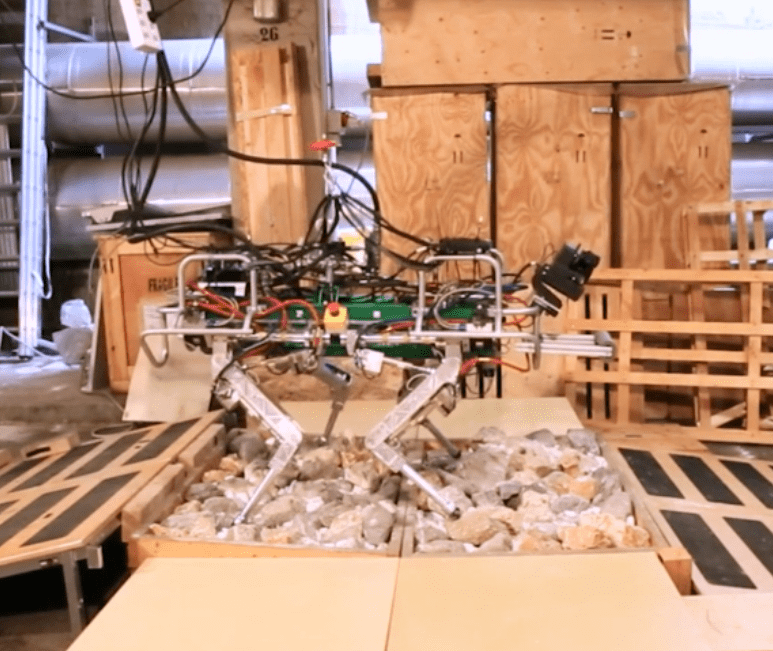
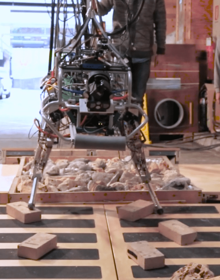
Figure 2: HyQ crawling on a rough terrain playground: (left) lateral and (right) frontal view. Our locomotion framework can deal with moving rocks and various terrain elevation changes.

I-B Echord++

This work is part of the Echord++ HyQ-REAL experiment, where novel quadrupedal locomotion strategies are being developed to be used on newly designed hydraulic robots. At the time of writing this manuscript, the HyQ-REAL robot was not yet fully assembled. Therefore, the framework is demonstrated on its predecessor version, HyQ. The major improvements of HyQ-REAL over HyQ are: more powerful actuators, full power autonomy (no tethers), greater range of motion, self-righting capabilities, fully enclosed chassis. The presented software framework can be easily run on both platforms, thanks to the kinematics/dynamics software abstraction layer presented in [32].

I-C Outline

The remainder of this paper is detailed as follows. In Section II we briefly present our statically stable gait framework; Sections III and IV, detail the body motion and swing motion phases of the gait, respectively; Section IV is particularly focused on the different stepping strategies, depending on the presence of a visual feedback; Section V describes the reactive modules for robust rough terrain locomotion; in Section VI, we present an improved terrain estimator; Section VII shows a strategy for stair climbing based on the proposed framework; in Section VIII, we describe the implementation of our disturbance observer; in section IX we address the conclusions.

II Locomotion Framework Overview

In this section, we briefly illustrate our statically stable crawling framework, (previously presented in [28]), enriched with additional features specific for rough terrain locomotion.

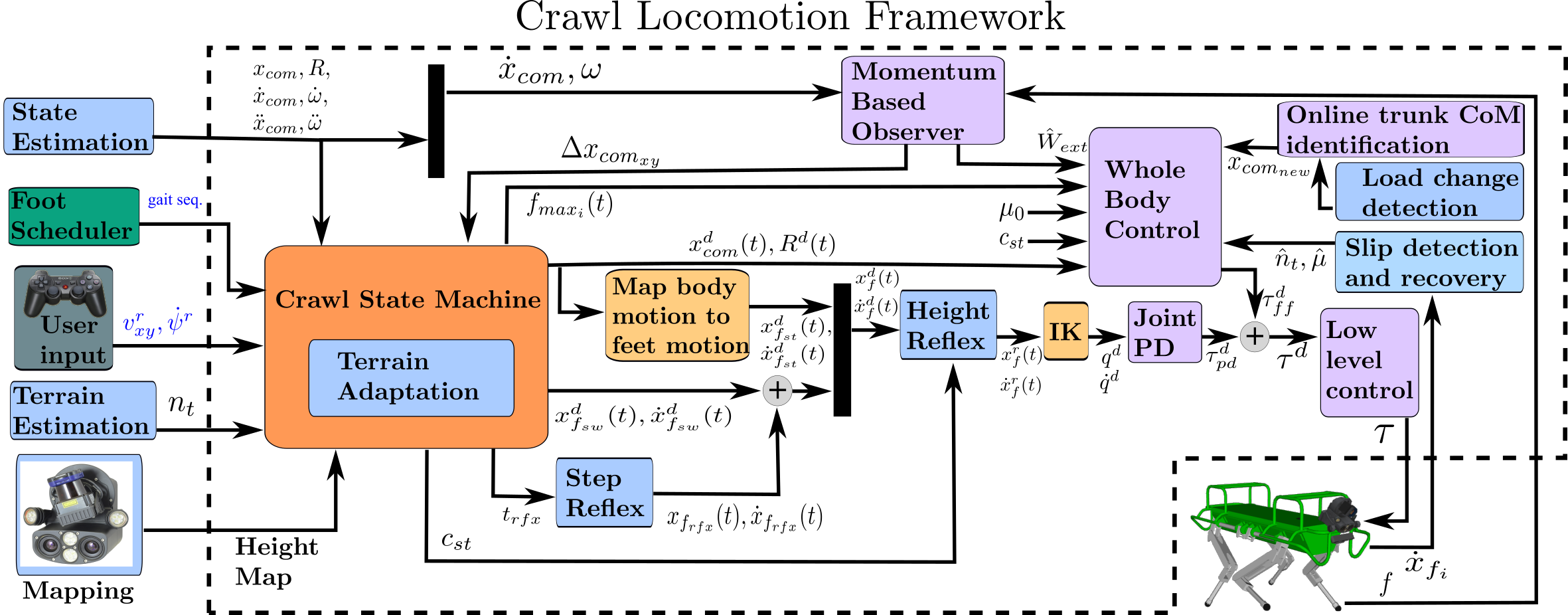
Figure 3: Block diagram of the crawl locomotion framework. The crawl state machine (orange block) is further detailed in Fig. 5. Please refer to $Appendix$ $B$ for a description of the main symbols shown in this figure.

Fig. 3 shows the block diagram of the framework. The core module is a state machine (see [28] for details) which orchestrates two temporized/event-driven locomotion phases: the swing phase, and the body motion phase. In the former, the robot has three legs in stance, while in the latter it has four legs in stance.

During the body motion phase, the robot Center of Mass (CoM) is shifted onto the future support triangle, (opposite to the next swing leg, in accordance to a user-defined foot sequence). As default footstep sequence we use: RH, RF, LH, LF.

The CoM trajectory is generated after the terrain inclination is estimated (see Section III). At each touchdown, the inclination is updated by fitting a plane through the actual stance feet positions. When the terrain is uneven (and the feet are not coplanar), an average plane is found.

The swing phase is a swing-over motion, followed by a linear searching motion (see Section IV) that terminates with a haptic touchdown. The haptic touchdown ensures that the swing motion does not stop in a prescheduled way; instead, the leg keeps extending until a new touchdown is established.

When a contact is detected (either by thresholding the Ground Reaction Force (GRF), or directly via a foot contact sensor [33, 34]), the touchdown is established. A searching motion with haptic touchdown is a key ingredient to achieve robust terrain adaptation. Indeed, haptic touchdown is important to mitigate the effect of tracking errors, because it allows to trigger the stance only when the contact is truly stable. This is important whenever there is a discrepancy between the plan and the real world. This typically happens when a vision feedback is used to select the foothold (see Section IV-B), because the accuracy of a height map is typically in the order of centimeters [27, 35].

The vision feedback can be also used to estimate the direction of the normal of the terrain under the foot, in order to set the searching, or reaching, motion direction. Both the body and the swing trajectories are generated as quintic polynomials.

The body trajectory is always expressed in the terrain frame, which is aligned to the terrain plane (see Fig. 4 (left)). The terrain frame has the $Z$-axis normal to the terrain plane, while the $X$-axis is a projection of the $X$-axis of the base on the terrain plane, and the $Y$-axis is chosen to form a right hand side system of coordinates. The swing trajectory is expressed in the swing frame, which can be either coincident with the terrain frame (section IV-A) or set independently for each foot (section IV-B), depending on the stepping strategy adopted.

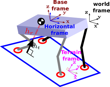
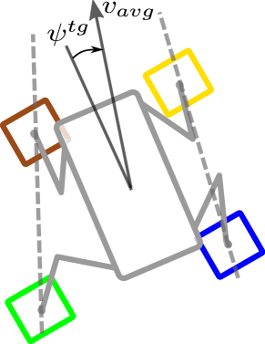
Figure 4: (left) Definition of the relevant reference frames and of the terrain plane (light blue) used in the locomotion framework and (right) computation of the target $\psi^{tg}$ for the robot yaw.

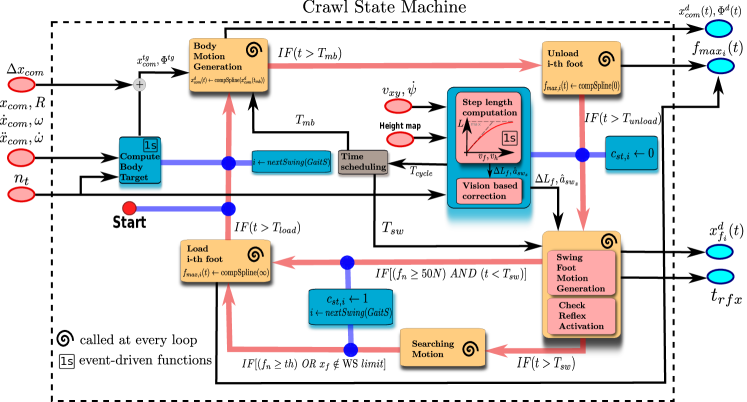
Figure 5: Logic diagram of the crawl state machine. The yellow rectangles represent the states, the red arrows represent the transitions while the blue boxes represent the actions associated to the transitions. Blocks marked with 1s (1-shot) are event-driven and perform a single computation, while the other blocks (marked with the spiral) are called every loop. Please refer to $Appendix$ $B$ for a short description of the main symbols shown in this figure.

The Whole Body Control module (also known as Trunk Controller [28]) computes the torques required to control the position of the robot CoM and the orientation of the trunk. At the same time, it redistributes the weight among the stance legs ($c_{st}$) and ensures that friction constraints are not violated.

The Trunk Controller action can be improved by setting the real terrain normal (under each foot) obtained from a 3D map [27], rather than using a default value for all the feet (e.g. the normal to the terrain plane). This is particularly important to avoid slippage when the terrain shape differs significantly from a plane.

To address unpredictable events (e.g. limit slippage on an unknown surface, whenever the optimized force is out of the real (unknown) friction cone), we implemented an impedance controller at the joint level [36] in parallel to the whole-body controller. The impedance controller computes the feedback joint torques $\tau_{fb}\in\mathbb{R}^{n}$ (where for HyQ $n=12$ is the number of active joints) to track reference joint trajectories $(q^{d}_{j},\leavevmode\nobreak\ \dot{q}^{d}_{j}\in\mathbb{R}^{n})$.

The sum of the output of the Trunk Controller $\tau_{ff}^{d}\in\mathbb{R}^{n}$ and of the impedance controller $\tau_{pd}^{d}\in\mathbb{R}^{n}$ form the torque reference $\tau^{d}\in\mathbb{R}^{n}$ for the low level torque controller. If the model is accurate, the largest term typically comes from the Trunk Controller.

Note that the impedance controller should receive position and velocity set-points that are consistent with the body motion, to prevent conflicts with the Trunk Controller. To achieve this, we map the CoM motion into feet motion (see Section III) to provide the correspondent joint references $q^{d}_{j},\leavevmode\nobreak\ \dot{q}^{d}_{j}$.

III Body Motion Phase

When traversing a rough terrain, unstable footholds (e.g. stones rolling under the feet), tracking errors, slippage and estimation errors can create deviations from the original motion plan. These deviations require some corrective actions in order to achieve terrain adaptation. In our framework, these actions are taken both at the beginning of swing and body motion phases. The body motion phase starts with a foot touchdown and ends when the next foot in the sequence is lifted off the ground. After each touchdown event, we compute the target for the CoM position $x_{com}^{tg}$ and the body orientation $\Phi^{tg}$ from the actual robot state. This feature prevents error accumulation and, together with the haptic touchdown, constitutes the core of the terrain adaptation feature.

To avoid hitting kinematic limits, the robot’s orientation should be adapted to match the terrain shape. Indeed, some footholds can only be reached by tilting the base. On the other hand, constraining the base to a given orientation restricts the range of achievable motions.

We parametrize the trajectory for the trunk orientation with Euler angles $\Phi^{d}(t)=[\phi(t)$, $\theta(t)$, $\psi(t)]$ (i.e. roll, pitch and yaw respectively). The trajectories are defined by quintic $3D$ polynomials connecting the actual robot orientation (at the beginning of the phase, namely the touchdown) $\Phi^{d}(0)=[\phi_{td},\theta_{td},\psi_{td}]$ with the desired orientation $\Phi^{d}(T_{mb})=\Phi^{tg}=[\phi^{tg},\theta^{tg},\psi^{tg}]$, where $T_{mb}$ is the duration of the move body phase. To match the inclination of the terrain, the target roll and pitch are set equal to the orientation of the terrain plane that was updated at the touchdown ($\phi^{tg}=\phi_{t},\theta^{tg}=\theta_{t}$). The target yaw $\psi^{tg}$ is computed to align the trunk with an average line $v_{avg}$ from the ipsi-lateral legs (see Fig. 4 (right)). This is somewhat similar to a heading controller that makes sure that the trunk “follows” the motion of the feet (the feet motion is driven by the desired velocity from the user).

Similarly to the angular case, the CoM trajectory is initialized with the actual position of the CoM , while the target $x_{com}^{tg}$ can be computed with different stability criteria (e.g. ZMP-based [1] or wrench-based [37, 38]). Henceforth, the vectors are expressed in the world (fixed) frame $\mathcal{W}$, unless otherwise specified.

Since the crawl does not involve highly dynamic motions, a heuristic static stability criterion can also be used and in particular, our strategy consists in making sure that the projection of the CoM target $x_{{com}_{p}}^{tg}$ always lies inside the future support triangle [28]. The robustness (in terms of stability margin) can be regulated by setting the projected $CoM$ target at a distance $d$, on the support plane, from the middle point of the segment connecting the diagonal feet (see Fig. 6 (right)). We define the robot height $h_{r}\in\mathbb{R}$ as the distance between the CoM and the terrain plane (see Fig. 4 (left)). This is computed by averaging the actual positions of the feet ${}_{b}x_{fi}$ in contact with the ground (stance feet):

$$h_{r}=e_{z}^{T}\frac{1}{c_{st}}\sum_{i=1}^{c_{st}}{}_{t}R_{b}({}_{b}x_{f_{i}}+{}_{b}x_{com})$$ (1)

where $c_{st}$ is the number of stance feet, ${}_{b}x_{com}\in\mathbb{R}^{3}$ is the CoM offset with respect to the base origin, ${}_{t}R_{b}\in SO(3)$ maps vectors from base to the terrain frame and $e_{z}\in\mathbb{R}^{3}$ selects the $Z$ component of $3D$ vectors. In general, the robot height should be kept constant (or it could vary with the cosine of the terrain pitch $\theta_{t}$ on ramps) during locomotion. If the above-mentioned heuristics is used for planning, the CoM target $x_{com}^{tg}$ can be obtained by adding the height vector expressed in the world frame $h_{r}n_{t}$ (where $n_{t}$ is the normal to the terrain) to the projection $x_{{com}_{p}}^{tg}$ coming from the heuristics.

Note that, on an inclined terrain, to have the CoM above the desired projection and the distance of the CoM from the terrain plane equal to $h_{r}$, the following scaling should be applied (see Fig. 6 (left)):

$$cos(\alpha)=e_{z}^{T}n_{t}$$ (2)

$$x_{com}^{tg}=x_{{com}_{p}}^{tg}+\frac{h_{r}}{cos(\alpha)}e_{z}$$

where $\alpha$ is the angle between the unit vectors $e_{z}$ and $n_{t}$.

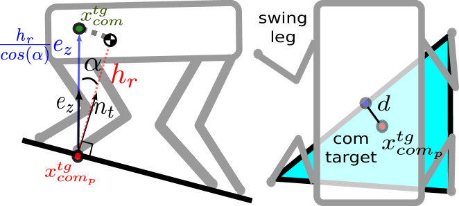
Figure 6: Heuristic generation of the CoM target. (left) planning on inclined terrain, (right) the future support polygon is depicted in light blue while the projection $x_{{com}_{p}}^{tg}$ of the com target on the polygon is a red dot.

Now, similarly to the orientation case, we build a quintic polynomial $x_{com}^{d}(t)$ to connect the actual CoM at the beginning of the motion phase (namely at the touchdown) $x_{com,td}$ to the computed target $x_{com}^{tg}$.

To determine the 6 parameters of each quintic, in addition to the initial/final positions, we force the initial/final velocities and accelerations to zero, both for CoM and Euler angles. This ensures static stability and implies that the robot’s trunk does not move when one leg is lifted from the ground (i.e. during the swing phase).

Alternatively, if a wrench-based optimization is used, as in [37], the robot height should be constrained (e.g. to be constant) and the CoM $X,Y$ trajectory will be a result of the optimization.

As mentioned in the previous section, it is convenient to provide desired joint positions (for the stance legs) that are consistent with the body motion. We first map the body motion into feet motion. This mapping is linear in the velocity domain and can be computed independently for each stance foot $i$ as:

$$\dot{x}_{f_{i}}^{d}[k]=-\dot{x}_{com}^{d}[k]-\omega[k]\times\left(x_{f_{i}}^{d}[k-1]-x_{com}([k]\right)$$ (3)

where the desired position of the foot $x_{f_{i}}^{d}[k-1]$ at the previous controller loop is used. Then, $x_{f_{i}}^{d}[k]$ is obtained by integrating the velocity $\dot{x}_{f_{i}}^{d}[k]$ (e.g. with a trapezoidal rule). Afterwards, we compute the corresponding desired joint positions $q_{i}\in\mathbb{R}^{3}$ through inverse kinematics: $q_{i}=IK(x_{f_{i}})$ and the joint velocities as:

$$\dot{q}^{d}_{i}=J(q_{i})^{-1}\dot{x}_{f_{i}}$$ (4)

where $J_{i}\in\mathbb{R}^{3\times 3}$ is the Jacobian of foot $i$.

IV Swing phase

The swing phase of a leg starts with the foot liftoff and ends with the foot touchdown. The obvious goal of the leg’s swing phase is to establish a new foothold. Then, an interaction force drives the robot’s trunk towards the desired direction. The swing phase has two main objectives: 1) attaining enough clearance to overcome potential obstacles (so as to avoid stumbling) and 2) achieving a stable contact.

IV-A Heuristic Stepping

In this section, we illustrate the heuristic stepping strategy we use for blind locomotion. The goal is to select the footholds to track a desired speed from the user when no map of the surroundings is available.

First, we compute the default step length (for the swing leg) from the desired linear and heading velocities $v_{xy}^{r}\in\mathbb{R}^{2},\;\dot{\psi}^{r}\in\mathbb{R}$. For sake of simplicity, only in this section the vectors are expressed in the horizontal frame $\mathcal{H}$ (instead of the world frame $\mathcal{W}$), unless otherwise specified. Expressing the default step in a horizontal frame allows to formulate the swing motion independently from the orientation of both terrain and trunk.

The swing trajectory consists of a parametric curve, whose four main parameters are: the linear foot displacement $\Delta L_{x0},\Delta L_{y0}$, the angular foot displacement $\Delta H_{0}$ (see Fig. 7), and the default swing duration $T_{sw}$. These quantities can be computed from the nonlinear mapping $F(\cdot)$:

$$\begin{bmatrix}\Delta L_{x0}&\Delta L_{y0}&\Delta H_{0}&T_{sw}\end{bmatrix}=F(v_{xy}^{r},\dot{\psi}^{r})$$ (5)

$F(\cdot)$ makes sure that the step lenght increments linearly with the desired velocity, but only at low speeds (see compute step length block in Fig. 5). When the step length approaches the maximum value, the cycle time $T_{cycle}$ (sum of swing and stance time of each leg) is decreased, and the stepping frequency $f_{s}=1/T_{cycle}$ is increased accordingly to avoid hitting the kinematic limits. For instance, for the $X$ component, we can use the following equation:

$$A =\frac{2\Delta L_{x0}^{max}}{\pi}$$ (6)

$$G =\frac{\Delta L_{x0}^{tr}}{\Delta L_{x0}^{max}v_{tr}}$$ (7)

$$\Delta L_{x0} =A\cdot\text{arctan}(Gv_{x}^{r})$$ (8)

where $\Delta L_{x0}^{max}$ is the maximum allowable step length in the $X$ direction.

According to Eq. (8), $\Delta L_{x0}$ linearly increases with velocity up to the transition point $\Delta L_{x0}^{tr}$, which corresponds to the user-defined value $v_{tr}$. Then, the step length is increased sub-linearly with velocity (because the stepping frequency is also increased), up to the saturation point $\Delta L_{x0}^{max}$. After this point, only the frequency increases. Similar computations are performed for $\Delta L_{y0}$ and $\Delta H_{0}$. Since it is possible to set different values for heading and linear speed, the cycle time (and so the stepping frequency) is adjusted to the minimum coming from the three velocity components:

$$T_{cycle}=min\left(\frac{\Delta L_{x0}}{v_{x}^{r}},\quad\frac{\Delta L_{y0}}{v_{y}^{r}},\quad\frac{\Delta H_{0}}{\dot{\psi}^{r}}\right)$$ (9)

When a new value of $T_{cycle}$ is computed, the durations of the body and swing trajectories are recomputed as $T_{mb}=(T_{cycle}-\leavevmode\nobreak\ T_{lu})D$ and $T_{sw}=(T_{cycle}-T_{lu})(1-D)$ respectively, according to the duty factor $D$ [39].

The variable $T_{lu}$ represents the cumulative duration of the load/unload phases. As explained in [28], we remark that a load/unload phase at the touchdown/liftoff events is important to avoid torque discontinuities. In particular, a load phase at the touchdown allows the Trunk Controller to redistribute smoothly the load on all the legs. At the same time, it ensures that the GRF always stay inside the friction cones, thus reducing the possibility of slippage.

Note that a heading displacement $\Delta H_{0}$ can be converted into a $X,Y$ displacement of the foot, as shown in Fig. 7, by:

$$\Delta L_{h0}=E_{xy}\begin{bmatrix}0&0&\Delta H_{0}\end{bmatrix}^{T}\times x_{\text{hip}}$$ (10)

where $x_{\text{hip}}\in\mathbb{R}^{3}$ is the vector from the origin of the base frame to the hip of the swinging leg, and $E_{xy}\in\mathbb{R}^{2\times 3}$ selects the $X,Y$ components.

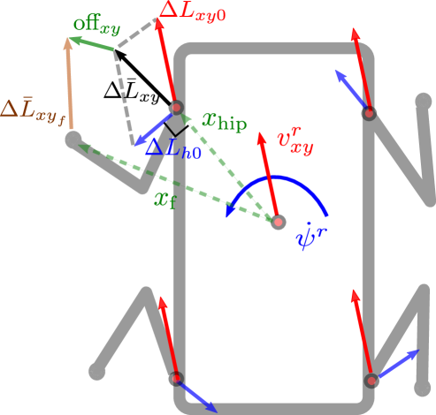
Figure 7: Vector definitions for the heuristic stepping strategy. Red arrows represent the desired linear velocity $v_{xy}^{r}$ and the linear component $\Delta L_{xy0}$ of the default step. In blue is the desired heading velocity $\dot{\psi}^{r}$ and the angular component $\Delta L_{{h0}}$ of the default step $\Delta\bar{L}_{xy0}$ that is in black. The offset to increase/decrease the stance size is in green, The step about the foot $\Delta L_{xy}$ is depicted in brown.

Then, the default step becomes:

$$\Delta\bar{L}_{xy0}=\Delta L_{xy0}+\Delta L_{{h0}}.$$ (11)

Note that we defined the default step about the hip rather than the foot position (see Fig. 7). This is crucial to avoid inconvenient kinematic configurations while walking (e.g. stretched or “crouched” configuration), thus degenerating the support polygon. Indeed, if we refer each step to the previous foot position, an anticipated/delayed touchdown would produce unexpected step lengths. This would make the stance feet closer/farther over time.

Since the swing polynomial is defined at the foot level, we have to determine the step $\Delta L_{xy}\in\mathbb{R}^{2}$ from $\Delta\bar{L}_{xy0}$, to express it about the actual foot position:

$$\Delta L_{xy}=\Delta\bar{L}_{xy0}+E_{xy}(\text{off}_{xy}+x_{hip}-x_{f}),$$ (12)

where $\text{off}_{xy}$ is a parameter to adjust the average size of the stance polygon.

In delicate situations, it might be useful to walk with the feet more outward to increase locomotion stability at the price of a bigger demanded torque at the Hip Abduction/Adduction (HAA) joint.

As a final step, it is convenient to express the swing motion in the swing plane (see Fig. 8). This means we need to express the above quantities in the swing frame $\mathcal{S}$.

We set quintic $3D$ polynomials $p(t)\in\mathbb{R}^{3}$ of duration $T_{sw}$, where the $X$, $Y$ components go from $(0,0)$ to ${}_{s}\Delta L_{xy}$, while for the $Z$ component we set two polynomials such that the swing trajectory passes by an intermediate apex point at a time $T_{sw}\chi$. At the apex, the $Z$ component is equal to the step height ${}_{s}\Delta L_{z}$ and $\chi\in[0,1]$ represents the apex ratio that can be adjusted to change the apex location (see Fig. 8). Hence, the swing foot reference trajectory is computed from the actual foot position at the instant of liftoff to the desired foothold as:

$$x_{f_{sw}}^{d}(\bar{t})=x_{f_{sw,lo}}+p(\bar{t}),$$ (13)

where $\bar{t}\in\begin{bmatrix}0&T_{sw}\end{bmatrix}$, $T_{sw}$ is the swing duration, and the final target is defined as $x_{f_{sw}}^{tg}=x_{f_{sw,lo}}+p(T_{sw})$.

Remark: the swing frame (unless specified) is always aligned with the terrain frame. Consequently, we have an initial retraction along the normal to the terrain plane (thus avoiding possible trapping or stumbling of the foot), while the step is performed along the terrain plane. A swing motion expressed in this way allows to adjust the step clearance simply with the step height ${}_{s}\Delta L_{z}$. This parameter regulates the maximum retraction from the terrain (apex point). In general, the apex is located in the middle of the swing, but it can be parametrized to shape differently the swing trajectory.

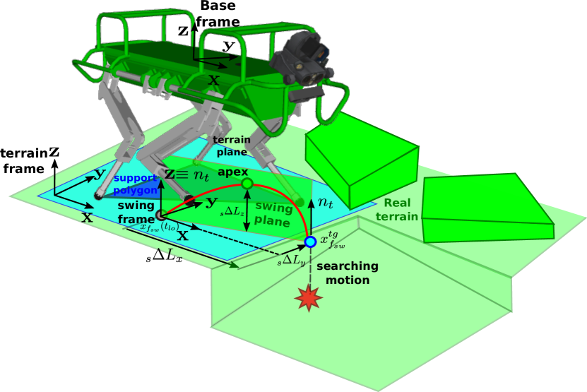
Figure 8: Swing frame and terrain frame definition for the heuristic-based stepping strategy used in blind locomotion. The terrain presents a decrease in elevation, haptically handled by the searching motion.

Definition: Searching motion. A haptic triggering of the touchdown allows to accommodate the shape of the terrain by stopping the swing motion either before of after the foot reaches the target $x_{f_{sw}}^{tg}$.

If the touchdown is deemed to happen after the target is reached, the trajectory is continued with a leg extension movement that we name searching motion: the swing foot keeps moving linearly along the direction of the terrain plane normal $n_{t}$ (see Fig. 8) until it touches the ground or eventually reaches the workspace (WS) limit. In this way, the stance is triggered in any case. To avoid mobility loss, a height reflex can be enabled to aid the search motion with the other stance legs (see section V-B).

IV-B Vision Based Stepping

The terrain plane is a very coarse approximation of the terrain. If a vision feedback is available, it is advisable to exploit this information, which allows to:

1. compute the target foothold on the actual terrain rather than on its planar approximation (see Fig. 9). This allows to increase the overall swing clearance (cf. blind stepping in Fig. 8 with vision based stepping in Fig. 9).

2. set a different swing frame for each foot instead of having the swing frame always coincident to the terrain frame. This enables the swing on different planes per each leg (essential for climbing though difficult terrain configurations such as V-shaped walls [28]).

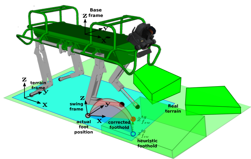
Figure 9: Swing frame definition for the vision-based stepping strategy. Blue and red shaded area represent the swing in the heuristic and the vision-based cases, respectively. In this case the terrain elevation is higher than the foot location at the liftoff and the target foot-hold (blue dot) computed with heuristics, is corrected by vision (red dot) to lay on the real terrain. The swing frame is also adjusted accordingly.

To implement the first point, we first compute a step (along the terrain plane) using the heuristic-based stepping strategy. This is meant to realize the user velocity. Then, the height map of the terrain is queried at the target location, and the $Z$ component of the target is corrected to have it on the real terrain ($X,Y$ components remain unchanged):

$$\tilde{x}^{tg}_{z}=H\left(E_{xy}x^{tg}_{f_{sw}}\right)$$ (14)

where $E_{xy}\in\mathbb{R}^{2\times 3}$ selects the X,Y components, and $H(\cdot)$ is a function that queries the terrain elevation for a certain (X,Y) location on the X-Y plane.

As a final step, we compute the $Z$ axis $\hat{a}_{{sw}_{z}}$ of the swing frame such that its $X$ axis $\hat{a}_{{sw}_{x}}$ is aligned with the segment connecting the actual foot position to the corrected foothold $\tilde{x}_{f_{sw}}^{tg}$ (see Fig 10):

$$a_{{sw}_{z}}=(\tilde{x}^{tg}_{f_{sw}}-x_{f_{sw}})\times({}_{w}R_{b}e_{y}),$$

$$\hat{a}_{{sw}_{z}}=\frac{a_{{sw}_{z}}}{\|a_{{sw}_{z}}\|},$$ (15)

$$\hat{a}_{{sw}_{y}}=\hat{a}_{{sw}_{z}}\times e_{x},$$

$$\hat{a}_{{sw}_{x}}=\hat{a}_{{sw}_{y}}\times\hat{a}_{{sw}_{z}},$$

where the $\hat{(\cdot)}$ represents unit vectors and $e_{x},e_{y}$ are the base frame axes expressed in the world frame. This correction allows for more clearance around the actual terrain during the swing motion and reduces the chances of stumbling.

The first consequence is that the swing frame is no longer aligned with the terrain frame, and the swing trajectory is laying on the plane $\hat{a}_{{sw}_{x}}/\hat{a}_{{sw}_{z}}$.

Additionally, if the normal $n_{r}$ of the actual terrain is available from the visual feedback [27], we can exploit it to further correct the swing plane, in order to have the swing-down tangent to that normal. This is particularly useful when the robot has to step on a laterally slanted surface (e.g. like in [28]).

In our experience, however, we noticed that on the sagittal direction, maximizing clearance has more priority. Therefore, we remove the component of $n_{r}$ along the $X$ axis computed in Eq. (IV-B) ($\hat{a}_{{sw}_{z}}^{v}=n_{r}-\hat{a}_{{sw}_{x}}^{T}n_{r})\hat{a}_{{sw}_{x}}$) and use as the new swing $Z$ axis. The new vision-corrected Z-axis of the swing frame becomes $n_{rp}$ (see Fig. 10), while the other axes should be recomputed accordingly as in Eq. (IV-B).

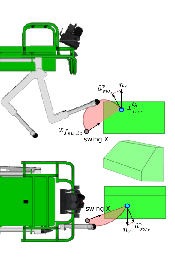
Figure 10: Vision based adjustment of the target foothold Z coordinate. Top and lateral views of the swing plane on a slanted terrain.

IV-C Clearance Optimization

If the quality of the map is good enough, the apex (point of maximum clearance) and the step height ${}_{s}\Delta L_{z}$ can be adjusted in accordance with the point of maximum asperity of the terrain, so as to maximize clearance. To some extent, this can be considered a simple adaptation of the swing to the terrain shape. First, we take a slice of the map and evaluate the height of the terrain on the line segment of direction $\hat{b}$ connecting the actual foot location with the target $\tilde{x}^{tg}_{f_{sw}}$ (see Fig. 11). With a discretization of $N$ points, we then follow the steps below:

$$1)\,\, s_{k}=\tilde{x}^{tg}_{f_{sw}}\frac{k}{N}+\tilde{x}_{f_{i}}\left(1-\frac{k}{N}\right),\quad k=1...N,$$

$$2)\,\, h_{k}=H(E_{xy}s_{k}),$$

$$3)\,\, \delta_{k}=\mathcal{P_{+}}(h_{k}-e_{z}^{T}s_{k}),$$ (16)

$$4)\,\, \delta_{k}^{\perp}=\left\|\begin{bmatrix}0&0&\delta_{k}\end{bmatrix}^{T}-\left(\begin{bmatrix}0&0&\delta_{k}\end{bmatrix}\hat{b}\right)\hat{b}\right\|,$$

$$5)\,\, \begin{bmatrix}{}_{s}\Delta L_{z}&k_{max}\end{bmatrix}=\max_{k}\delta_{k}^{\perp},$$

where 1) is a discretization of the line segment; 2) is the evaluation of the height map on the discretized points; 3) $\mathcal{P_{+}}(\cdot):\mathbb{R}\rightarrow\mathbb{R}$ is a function that sets negatives values to zero; in 4) we project the $\delta_{k}$ onto the swing $Z$ axis, getting $\delta_{k}^{\perp}$; in 5) we set the step height ${}_{s}\Delta L_{f_{sw}}$ as the maximum value among the $\delta_{k}^{\perp}$ where $k_{max}$ is its index. Finally, the apex can be set to $k_{max}/N$. This reshapes the swing in a conservative way, by adjusting the apex according to the terrain feature.

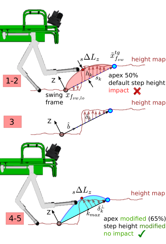
Figure 11: Clearance optimization. The grey dot represents the actual foot location at liftoff, the blue dot the foot target while the red dot the apex location. The numbers in the red rectangles are related to the steps in Eq. (IV-C).

IV-D Time Rescheduling

In our state-machine-based framework, a change in locomotion speed corresponds to changing the duration of the swing/body phases. However, to change speed promptly (without waiting until the end of the current phase) it is necessary to reschedule the polynomials of the active phase (swing or body motion). As a consequence, we compute a new duration $T_{f}^{{}^{\prime}}$ (where $T_{f}$ is the previous duration). Setting a new duration for a (previously designed) polynomial is equivalent to finding the initial point of a new polynomial that: 1) has the new duration $T_{f}^{{}^{\prime}}$ and 2) is passing through the same point at the moment of the rescheduling. We know that a quintic polynomial can be expressed as:

$$p(t)=a^{T}\mu(t),\quad\dot{p}(t)=a^{T}\dot{\mu}(t),\quad\ddot{p}(t)=a^{T}\ddot{\mu}(t)$$ (17)

where:

$$a^{T}=\begin{bmatrix}a_{5}&a_{4}&a_{3}&a_{2}&a_{1}&a_{0}\end{bmatrix},$$ (18)

$$\mu(t)=\begin{bmatrix}t^{5}&t^{4}&t^{3}&t^{2}&t&1\end{bmatrix},$$

$$\dot{\mu}(t)=\begin{bmatrix}5t^{4}&4t^{3}&3t^{2}&2t&1&0\end{bmatrix},$$

$$\ddot{\mu}(t)=\begin{bmatrix}20t^{3}&12t^{2}&6t&2&0&0\end{bmatrix}.$$

Setting the initial/final boundary conditions for position, velocity and acceleration: $p_{0}=a^{T}\mu(0)$, $\dot{p}_{0}=a^{T}\dot{\mu}(0)$, $\ddot{p}_{0}=a^{T}\ddot{\mu}(0)$, $p_{f}=a^{T}\mu(T_{f})$, $\dot{p}_{f}=a^{T}\dot{\mu}(T_{f})$, $\ddot{p}_{f}=a^{T}\ddot{\mu}(T_{f})$ is equivalent to solving a linear system of $6$ equations that allows us to find the $a_{i}$ parameters:

$$a_{0}=p_{0},$$ (19)

$$a_{1}=\dot{p}_{0},$$

$$a_{2}=0.5\ddot{p}_{0},$$

$$a_{3}=\frac{1}{2T_{f}^{3}}\left[20p_{f}-20p_{0}+T_{f}(-12\dot{p}_{0}-8\dot{p}_{f})+T_{f}^{2}(-3\ddot{p}_{0}+\ddot{p}_{f})\right],$$

$$a_{4}=\frac{1}{2T_{f}^{4}}\left[30p_{0}-30p_{f}+T_{f}(16\dot{p}_{0}+14\dot{p}_{f})+T_{f}^{2}(3\dot{p}_{0}-2\dot{p}_{f})\right],$$

$$a_{5}=\frac{1}{2T_{f}^{5}}\left[12p_{f}-12p_{0}+T_{f}(-6\dot{p}_{0}-6\dot{p}_{f})+T_{f}^{2}(-\ddot{p}_{0}+\ddot{p}_{f})\right],$$

with a similar criterion, to ensure continuity in the position, we can compute the new initial point $p_{0}^{\prime}$ such that:

$$a^{\prime}\mu(\bar{t})=p(\bar{t}),$$ (20)

where $\bar{t}$ is the time elapsed (from $0$) at the moment of the rescheduling, and $a^{\prime}$ are the coefficient of the new polynomial of duration $T_{f}^{{}^{\prime}}$. Then, collecting $p_{0}$ from all the parameters in Eq. (19), we can obtain a closed form expression for it:

$$\beta_{1}=\frac{1}{2T_{f}^{3}}\left[20p_{f}+T_{f}(-12\dot{p}_{0}-8\dot{p}_{f})+T_{f}^{2}(-3\ddot{p}_{0}+\ddot{p}_{f})\right],$$

$$\beta_{2}=\frac{1}{2T_{f}^{4}}\left[-30p_{f}+T_{f}(16\dot{p}_{0}+14\dot{p}_{f})+T_{f}^{2}(3\dot{p}_{0}-2\dot{p}_{f})\right],$$

$$\beta_{3}=\frac{1}{2T_{f}^{5}}\left[12p_{f}+T_{f}(-6\dot{p}_{0}-6\dot{p}_{f})+T_{f}^{2}(-\ddot{p}_{0}+\ddot{p}_{f})\right],$$

$$\beta_{4}=1-10T_{f}^{3}\bar{t}^{3}+15T_{f}^{4}\bar{t}^{4}-6T_{f}^{5}\bar{t}^{5},$$

$$p_{0} =\frac{1}{\beta_{4}}\left[p(\bar{t})-a_{1}\bar{t}+a_{2}\bar{t}^{2}+\beta_{1}\bar{t}^{3}+\beta_{2}\bar{t}^{4}+\beta_{3}\bar{t}^{5}\right]$$ (21)

Now, exploiting Eq. (IV-D) for the computation of $p_{0}$, the new polynomial parameters can be recomputed as in Eq. (18) while keeping the other boundary conditions unchanged. This will result in a polynomial that continues from $\bar{t}$ with a new duration $T_{f}^{{}^{\prime}}$.

In Fig. 12, we show an example of time rescheduling happening at $0.5s$, where the duration of an original trajectory $T_{f}=1s$ is reduced to $T_{f}^{{}^{\prime}}=0.7s$ (fast scheduling) or increased to $T_{f}^{{}^{\prime}}=1.5s$ (slower scheduling).

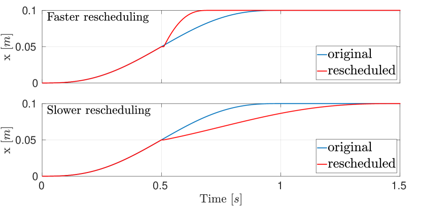
Figure 12: Time rescheduling. The original trajectory (blue) at $\bar{t}=0.5s$ is rescheduled into a new trajectory (red) of duration of (Upper plot) $0.7s$ or (lower plot) $1.5s$.

V Reactive Behaviors

In this section, we briefly describe the framework’s reactive modules for robust locomotion. These modules implement strategies to mitigate the negative effects of unpredictable events, such as: 1) slippage (Section V-A); 2) loss of mobility (Section V-B); 3) frontal impacts (see Section V-C) and 4) unexpected contacts (e.g. shin collisions, see Section V-D).

V-A Slip Detection

The causes of slippage during locomotion can be divided into three categories: 1) wrong estimation of the terrain normal; 2) wrong estimation of the friction coefficient; 3) external disturbances.

In our previous work [24], we addressed the first and the second categories. In particular, we proposed a slippage detection algorithm which estimates online the friction coefficient and the normal to the terrain. After the estimation, the coefficient were passed to the whole-body controller (see slip detection and recovery module in Fig. 3).

Concerning the third category, an external push can create a loss of contact. This can cause a sudden inwards motion of the foot. For instance, the trunk controller can create internal forces, depending on the regularization used. When there is loss of contact, these internal forces can make the foot move away from the desired position, leading to large tracking error and catastrophic loss of balance. Thanks to the impedance controller (a PD running in parallel to the Trunk Controller), the tracking error will be limited, and it will be recovered at the next replanning stage (see Section III).

V-B Height Reflex

The height reflex is a motion generation strategy for all the robot’s feet. It redistributes the swing motion onto the stance legs, with the final effect of “lowering” the trunk to assist the foothold searching motion.

The height reflex is useful when the robot is facing considerable changes in the terrain elevation (e.g. stepping down from a high platform) [29]. In such situations, the swing leg can lose mobility, causing issues during the subsequent steps (e.g. walking with excessively stretched legs). For this reason, the height reflex is most likely to be activated when stepping down.

V-C Step Reflex

The step reflex [30] is a local elevation recovery strategy, triggered in cases of frontal impacts with an obstacle during the swing up phase.

This reflex is key in cases of visual deprivation (e.g. smoky areas or thick vegetation): it allows the robot to overcome an obstacle and establish a stable foothold at the same time, without stumbling.

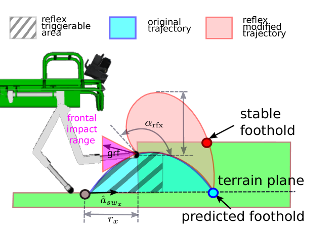
Figure 13: Step Reflex. In shaded blue the original trajectory while in shaded red is the modification due to the reflex. The red cone, shows the range of GRF that are eligible as frontal impacts. Out of this cone the GRF will be used to trigger the stance. Area of possible activation along the trajectory, is depicted with stripes.

Since the step reflex can be enabled only during the swing phase, it is important to set its duration $T_{\text{rfx}}$ to stop concurrently with the end of the default swing duration:

$$T_{\text{rfx}}=T_{sw}-\bar{t},$$ (22)

where $\bar{t}$ is the time elapsed from the beginning of the swing until the moment the reflex is triggered (the searching motion will be still possible to accommodate for further errors).

The angle of retraction $\alpha_{\text{rfx}}$ (see Fig. 13) depends on the distance $r_{x}$ (along the swing $X$ axis $\hat{a}_{{sw}_{x}}$ of the swing frame) already covered by the swing foot:

$$r_{x}=\hat{a}_{{sw}_{x}}^{T}(x_{f_{sw}}^{d}(\batchmode{\bar{t}})-x_{f_{sw}}^{d}(0)),$$ (23)

and the reflex maximum vertical retraction $r_{z}$:

$$\alpha_{\text{rfx}}=\operatorname{atan2}(r_{z},r_{x}).$$

The maximum vertical retraction $r_{z}$ is an input parameter related to the step height and the roughness of the terrain. Note that the step reflex is also conveniently generated in the swing frame.

The reflex can be triggered only when the impact is frontal (GRF in the purple cone of Fig. 13), and only during the swing up phase (e.g. before the apex point). The reason for these constraints is twofold:

1. a force from a frontal impact is larger (and pointing downwards) if the impact occurs in the swing up phase; in contrast, it is lower (and pointing upwards) in the swing down phase. Therefore, a small and upward force would cause an increment of false positives for a regular touchdown detection.

2. the time available for a reflex after the swing apex is more limited and would require significantly higher accelerations to be executed.

Missed reflex: If a frontal impact is detected in the swing down phase, the reflex is not triggered immediately, but it is scheduled for the beginning of the next swing phase.

The accompanying video shows a simulation where the robot performs a blind stair ascent, using the heuristic-based stepping strategy as described in Section IV-A). Even if the swing leg stumbles against the step, the robot is still able to climb the stairs, thanks to the step reflex. In contrast, when the step reflex is disabled, the robot gets stuck.

Remark: the reflex is omni-directional and depends on the desired locomotion speed. For instance, if the robot walks sideways, the step will be triggered along the swing-plane, which will be oriented laterally.

V-D Shin Collision

The foot might not be the only point of contact with the terrain. For certain configurations, the shin of a quadruped robot can collide as well (as shown in this simulation ). Since contact forces directly influence the dynamics of the robot, we take this into account in the trunk controller, i.e. with an appropriate weight redistribution after updating the number and location of the contact points. The detection of the contact point location can be done either with a dedicated sensor or an estimation algorithm. On the same line, the contact points are updated during the generation of body trajectories.

V-E Experimental Results

In this section, we present the experiments carried out on our robotic platform HyQ, to show the effectiveness of the proposed reactive behaviors framework in addressing rough terrain locomotion. All the experiments have been carried out on HyQ, a $85\text{\,}\mathrm{kg}$, fully-torque controlled, hydraulically actuated quadruped robot [40].

HyQ is equipped with a variety of sensors, including: precision joint encoders, force/torque sensors, a depth camera (Asus Xtion), a combined (stereo and LiDAR) vision sensor (MultiSense SL), and a tactical grade Inertial Measurement Unit (KVH 1775).

The size of HyQ is $1.0\text{\times}0.5\text{\times}0.98\text{\,}\mathrm{m}$ (L $\times$ W $\times$ H). The leg’s length ranges from $0.339\text{\,}\mathrm{m}$ to $0.789\text{\,}\mathrm{m}$ and the hip-to-hip distance is $0.75\text{\,}\mathrm{m}$.

HyQ has two onboard computers: a real-time compliant (Xenomai-Linux) used for locomotion and a non-RT machine to process vision data. The RT PC processes the low-level controller (hydraulic actuator controller) at $1\text{\,}\mathrm{kHz}$ and communicates with sensors and actuators through EtherCAT. Additionally, this PC runs the high-level controller at $250\text{\,}\mathrm{Hz}$ and the state estimation at $500\text{\,}\mathrm{Hz}$. The non-RT PC processes the exteroceptive sensors to generate a 2.5-D terrain map [42] with $4\text{\,}\mathrm{cm}$ resolution and $3\text{\times}3\text{\,}\mathrm{m}$ size, surrounding the robot.

The template terrain used for the experiments is shown in Fig. 2. It is composed by: 1) ascending ramp; 2) a step-wise elevation change; 3) area with big stones (diameter up to $12\text{\,}\mathrm{cm}$); 4) another step-wise elevation change; 5) a descending ramp with random bricks. Walking on stones and bricks is challenging from the locomotion point of view: the stones can collapse or roll away, causing a loss of balance, if specific strategies are not implemented. This video shows the robot successfully traversing the template terrain. The terrain adaptation capabilities (e.g. haptic feedback, searching motion) are mostly demonstrated when the robot is walking on rocks. The changes in elevation (where the height reflex is triggered) prevents the swing leg from losing mobility.

The importance of replanning is particularly evident during the stair descent, where the robot steps on bricks rolling away under a foothold. The pitch error caused by the rolling bricks is recovered in the next step. Since the crawl is statically stable, the robot can move in extremely cluttered environments, almost at ground level. In the last scene of the video, we show a simulation with the second generation of our robots, HyQ2Max [43]. Thanks to its increased range of motion with respect to HyQ, this robot is able to crawl with a very low desired body height and is thus able to walk through $45\text{\,}\mathrm{cm}$ wide duct.

VI Terrain Estimation

The terrain estimation module (see Fig. 3) estimates the terrain plane, which is a linear approximation of the terrain enclosed by the stance feet.

The inclination of the terrain plane ($\phi_{t}$,$\theta_{t}$) is updated at each touchdown event (e.g. a when a foot is “sampling” the terrain). Typically, this is done by fitting a plane through the stance feet and computing the principal directions of the matrix containing the feet positions. The fitting plane can be found in two ways:

• Vertical Fit: it minimizes the “distance” along the vertical component, between the fitting plane ($\Pi:ax+by+cz+d=0$) and the set of points represented by the feet position;

• Affine Fit: it minimizes the Euclidean distance (along the terrain plane normal) between the feet and the plane.

In the first case, we have to solve a linear system, while the second is an eigenvalue problem.

VI-A Vertical Fit

The “vertical” distance can be minimized by setting the $c$ coefficient to be equal to 1 and solve a linear system for the $x=\begin{bmatrix}a&b&d\end{bmatrix}$ parameters:

$$x=A^{\text{\#}}b,$$ (24)

where the positions of the stance feet have been collected in:

$$A=\begin{bmatrix}x_{f_{1x}}&x_{f_{1y}}&1\\ x_{f_{2x}}&x_{f_{2y}}&1\\ x_{f_{3x}}&x_{f_{3y}}&1\\ x_{f_{4x}}&x_{f_{4y}}&1\end{bmatrix},\quad b=\begin{bmatrix}-x_{f_{1z}}\\ -x_{f_{2z}}\\ -x_{f_{3z}}\\ -x_{f_{4z}}\end{bmatrix}.$$ (25)

and where $[\cdot]^{\#}$ is the Moore-Penrose pseudoinverse operator. Then, the normal to the terrain plane $n_{t}$ and the correspondding roll/pitch angles $\phi_{t},\theta_{t}$ (in ZYX convention), can be obtained as:

$$n_{t} =\begin{bmatrix}a&b&1\end{bmatrix}^{T}/\|\begin{bmatrix}a&b&1\end{bmatrix}\|,$$

$$\theta_{t} =\operatorname{atan}(n_{t_{x}}/n_{t_{z}}),$$ (26)

$$\phi_{t} =\operatorname{atan}(-n_{t_{y}}\sin(\theta_{t})/n_{t_{x}}).$$

VI-B Affine Fit

In the affine case, we first need to reduce the feet samples by subtracting their average $\bar{x}$ (belonging to the fitting plane):

$$R=\begin{bmatrix}x_{f_{1}}^{T}-\bar{x}^{T}\\ x_{f_{2}}^{T}-\bar{x}^{T}\\ x_{f_{3}}^{T}-\bar{x}^{T}\\ x_{f_{4}}^{T}-\bar{x}^{T}\end{bmatrix},\quad\bar{x}=\frac{1}{4}\sum_{i=1}^{4}x_{f_{i}}.$$ (27)

The principal directions of this set of samples are the eigenvectors of $R^{T}R$:

$$\begin{bmatrix}V&D\end{bmatrix} =eig\left(R^{T}R\right)$$

$$n_{t} =S_{1}V$$ (28)

where $V$ is the matrix of the eigenvectors and $D$ the diagonal matrix of the eigenvalues of $R^{T}R$.

We can obtain the terrain normal $n_{t}$ by extracting the first column from the eigenvector matrix (e.g. the eigenvector associated to the smallest eigenvalue). Then, similarly to the vertical fit case, Eq. (VI-A) can be applied to find the terrain parameters. Note that the result is slightly different from the vertical fit case. Indeed, in the affine fit case, we minimize the Euclidean distance, while in the vertical fit case we minimize the distance along the $z$ direction. On the other hand, the two approaches give the same result if the feet are coplanar.

It is noteworthy that the affine approach does not provide meaningful results when $R^{T}R$ is rank deficient. However, this happens only when (at least) three feet are aligned, which is a very unlikely situation.

VI-C Correction for Rough Terrain

There are some situations where just fitting an average plane is not the ideal thing to do during a statically stable motion. For instance, when the robot has three feet on the ground and one on a pallet, the average (fitting) plane is not horizontal. In this case, moving the CoM projection along the terrain plane (to enter in the support triangle) results in an inconvenient “up and down” motion. This happens because the robot tries to follow the orientation of the terrain plane with its torso. In this case, it would be preferable to keep the posture horizontal until at least two feet are on the pallet.

In this section, we propose a more robust implementation of the terrain estimation strategy, which allows to address these particular situations. The idea is to have the terrain plane fitting the subset of the stance feet that are closer to be coplanar. In this case, the influence of the “outlier” foot (e.g. the one on the pallet) would be reduced. For more dynamic gaits, where the CoM trajectory is not planned (e.g. like trotting [23]), a low-pass filtering of the terrain estimate would be sufficient to mitigate the effect of the outliers. However, since the crawl makes heavily use of the terrain plane to change the pose of the robot, a different strategy has be adopted.

A preliminary step (after computing the terrain normal $n_{t}$ as in Section VI-A) is to compute the norm of the least square errors vector. This can be easily done by exploiting the matrix computed in Eq. (25): $e_{LS}=\|Ax-b\|_{2}$. If $e_{LS}$ (Least Square error) is bigger than a certain (user defined) threshold, it means that the feet are not coplanar, and $n_{t}$ should be corrected.

First, we compute the normal vectors in common to all the combinations of two adjacent edges ($l_{i}$, $l_{j}$), (sorted in Counter Clock Wise (CCW) order, see Fig. 14):

$$n_{ij}=l_{i}\times l_{j}\quad(i,j)\in C,$$ (29)

where $C$ is the set of all the combinations of two adjacent edges (sorted in CCW order). In our case, $C$ has 4 elements. Since any couple of (intersecting or parallel) lines defines a plane, we associate each normal $n_{ij}$ to one support triangle (e.g. two edges of the support polygon, see Fig. 14 (left)).

The corrected terrain normal is a weighted average of $n_{ij}$, where the weights are inversely proportional to the distance of each normal $n_{ij}$ from the terrain plane normal, computed at the previous touchdown event $n_{t_{{}_{\textup{old}}}}$.

$$cos(\alpha_{ij})=n_{t_{old}}^{T}n_{ij}.$$ (30)

We compute the weight $w_{ij}$ associated to each normal $n_{ij}$ through the nonlinear function $W(\cdot)\in\mathbb{R}\rightarrow\mathbb{R}$ (Fig. 14 (right)), in accordance to its angular distance from $n_{t_{{}_{\textup{old}}}}$.

$$W(x)=1/\left(1+s(x-1)^{p}\right),$$

$$w_{k}=W(cos(\alpha_{ij})),$$ (31)

where $k$ is the index of the $ij-th$ element of the set $C$; and $s$ is a sensitivity factor proportional to the LS error $e_{LS}$.

According to Eq. (31), the normals closer to $n_{t{{}_{\textup{old}}}}$ (e.g. cosine close to 1) are assigned a bigger weight (the weight is bounded to 1 by construction of $W(\cdot)$). The exponent $p$ allows us to adjust the degree of nonlinearity of $W(\cdot)$ and the degree of correction (in our case $p=2$ was sufficient).

Since the normals $n_{ij}$ are directly affected by the position of their corresponding feet on the pallet, a weighted average of the normals (with weights inversely proportional to the distance from the previous estimation) allows to naturally reduce the influence of the “outlier” foot. This discourages the terrain estimator from modifying too much the previous estimate when a foot position is far away from the previous fitting plane.

Note that, since we are aiming at “averaging” orientations, we need to perform a Spherical Linear intERPolation (SLERP) using geodesic curves [44] (see $Appendix$ $A$).

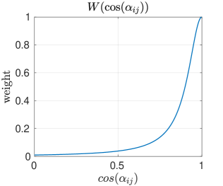
Figure 14: Smart height correction. (Left) the blue arrow represent the corrected normal while the grey arrow the not corrected one (computed with the affine fit method). In this case the corrected normal is almost coincident to one of the red arrows representing the normals $n_{ij}$ to the triangles defined by three stance feet; (right) weight function (W) of the angular distance (e.g. cosine) w.r.t $n_{t_{old}}$.

VI-D Experimental Results

The terrain estimation video shows how the smart terrain estimator improves locomotion by removing undesired up/down motions.

With reference to our initial example, as long as the robot has one foot on the pallet, the normal is closer to the one provided by the other stance feet — which in turn are closer to the previous estimation with all the feet on the flat ground (see Fig. 14).

When the robot steps with the two lateral feet on the pallet, the fitting error $e_{LS}$ is reduced (the feet are more coplanar) and an inclined terrain plane is estimated.

The approach can address situations with non coplanar feet (e.g. support has a “diamond” shape, shown later in the video). In this case, the terms from the feet on the pallet cancel each other, keeping the previous terrain plane estimate unchanged, which is the desirable behavior. For the single pallet example, we have $e_{LS}=0.02$ (for the “diamond” shape $e_{LS}=0.031$), therefore we set the threshold of intervention for the terrain correction to $0.002$.

Since we want a stronger correction when the $LS$ error increases, we make the sensitivity factor $s$ of the function $W(\cdot)$ proportional to $e_{LS}$.

VII Stair climbing

Stair climbing is an essential skill in the for a legged robot. Indeed, a versatile legged robot should be able to address both unstructured and structured environments, such as the one we can find in a disaster scenario.

The problem of stair climbing can be addressed through foothold planning, to avoid collisions with the step edges. An optimization taking into account the full kinematic of the robot could possibly solve the problem, but it is currently hard to be performed online.

Moreover, as previously mentioned, a full optimization approach that plans for a whole staircase is prone to tracking errors, which might eventually end up in missing a step and fall.

An alternative strategy is to conservatively select the foothold in the middle of the step (depth-wise). However, depending on the inclination of the stairs and on the step-size, the robot can end up in inconvenient configurations from the kinematic point of view (e.g. with degeneration of the support triangle and associated loss of mobility).

In the case of HyQ, the kinematic limits at the Hip-Flexion-Extension joints (i.e. hip joints rotating around the $Y$-axis, see [40]) are likely to be hit during the body motion phase.

According to our experience, keeping the joint posture as close as possible to the default configuration it improves mobility, and is an important factor for the robustness of locomotion. Our heuristic approach, rather than avoiding potentially dangerous situations (e.g. missed steps, collisions), aims to be robust enough to cope with them.

In particular, we show that our vision-based stepping approach, with minor modifications (see section VII-B), is sufficient to successfully climb up/down industrial-size stairs. In case the vision based swing strategy is not sufficient to avoid frontal impacts (e.g. against one step), the step reflex is triggered to achieve a stable foothold and prevent the robot from getting stuck.

VII-A Influence of the knee configuration

The probability of “getting stuck” when climbing stairs depends on the knee configuration (bent backwards or forward). In particular, when the leg has a Knee Bent Backward (KBB) configuration, it is more prone to have shin collision when climbing downstairs. Conversely, a Knee Bent Forward (KBF) configuration increases the risk of shin collision when climbing upstairs. These are important aspects for the design of robots that are expected to climb stairs.

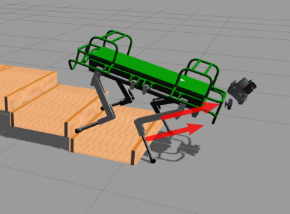
Figure 15: Comparison of KBB and KBF configurations during stair climbing. In the KBF while climbing up the GRF point against the direction of motion making the robot get stuck.

Note that the contact forces at the shin are in the direction of motion when the configuration is KBB and the robot is climbing downstairs, whereas they point against the motion with the KBF configuration and the robot climbs upstairs (see Fig. 15). In the former case we might have slippage, but the robot eventually moves forward, while in the latter case the robot might get stuck or fall backwards, unless these situation are properly dealt with (see Section V-D).

VII-B Stair locomotion mode

The stair locomotion mode can be triggered either by the user or by a dedicated stair detection algorithm [46]. It consists in the activation of three features (relevant for the task of climbing stairs) on top of the vision-based stepping strategy:

1. Rescheduling of the gait sequence: the kinematic configurations that cause mobility loss are undesired. To avoid them, it is important to climb stairs with both front feet (or back feet) on the same step. Specifically, the next foot target is checked at each touchdown (i.e. before the move body phase). If this is on a different height than the foot on the opposite side, we perform a rescheduling of the gait sequence.

   For instance, if the last swing foot was the right front ($RF$) then, according to our default configuration ($RH,RF,LH,LF$) the next leg to swing would be the $LH$. However, if the left-front ($LF$) foot is on a different height (e.g. still on the previous step), the whole sequence is rescheduled to move the $LF$ instead. The same applies for the back feet.

2. Conservative stepping: taking inspiration from the ideas presented in [25], this module corrects the foot location to step far away from an edge. The terrain flatness is checked along the direction of motion and the foothold is corrected (along the swing plane) in order to place it in a more conservative location (i.e. away from the step edge).

3. Clearance optimization: this feature (presented in Section IV-C) is useful to avoid the chance of stumbling against the step’s edge. It adjusts the swing apex and the step height to maximize the clearance from the step.

VII-C Experimental Results

We successfully applied the reactive modules of our framework to the problem of climbing up (and down) stairs, in simulation, with our quadruped robot, HyQ. In the video, we show that HyQ is able to climb up and down industrial size stairs (step raise $14\text{\,}\mathrm{cm}$) and climbing up a staircase with a $90\text{\,}\mathrm{\SIUnitSymbolDegree}$ turn.

The approach is generic enough to be used also with irregular stair patterns (different step raise) and turning stairs. The user provides only a reference speed and heading.

In the simulation video we show the advantage of activating the stair locomotion mode and the importance of using a vision based stepping strategy.

In the $90\text{\,}\mathrm{\SIUnitSymbolDegree}$ staircase, we demonstrate omni-directional capability of our statically stable approach, which allows to move backwards on the staircase.

VIII Momentum Based Disturbance Observer

A significant source of error might come from unmodeled disturbances, such as an external push. Specifically, in the case of a model-based controller (e.g. our Whole Body controller [28]), inaccurate model parameters cause a wrong prediction of the joint torques. This shifts the responsibility of the control to the feedback-based controllers, thus increasing tracking errors and delays. However, if a proper identification is carried out offline, these model inaccuracies are mainly restricted to the trunk. Indeed, in the case of our quadruped robot, the leg inertia does not change significantly, but the trunk parameters are instead strongly dependent on robot payload (e.g. a backpack, an additional computer, different sets of cameras for perception, etc.).

In [48], we presented a recursive strategy which performs online payload identification to estimate the new CoM position of the robot’s trunk. The updated model is then used for a more accurate inversion of the dynamics [28, 3]. Even though this approach is effective to detect constant payload changes, it is not convenient to estimate time-varying unknown external forces, which might change both in direction and intensity. Indeed, this kind of disturbances can dramatically increase the tracking errors and jeopardize the locomotion, unless they are compensated online.

In the following, we mention two scenarios where an external disturbance observer is useful: 1) the robot is required to pull a cart or a load (e.g. with some delicate material inside); and 2) the robot is requested to pull up a payload from underneath with a hoist mounted on the torso (see 16).

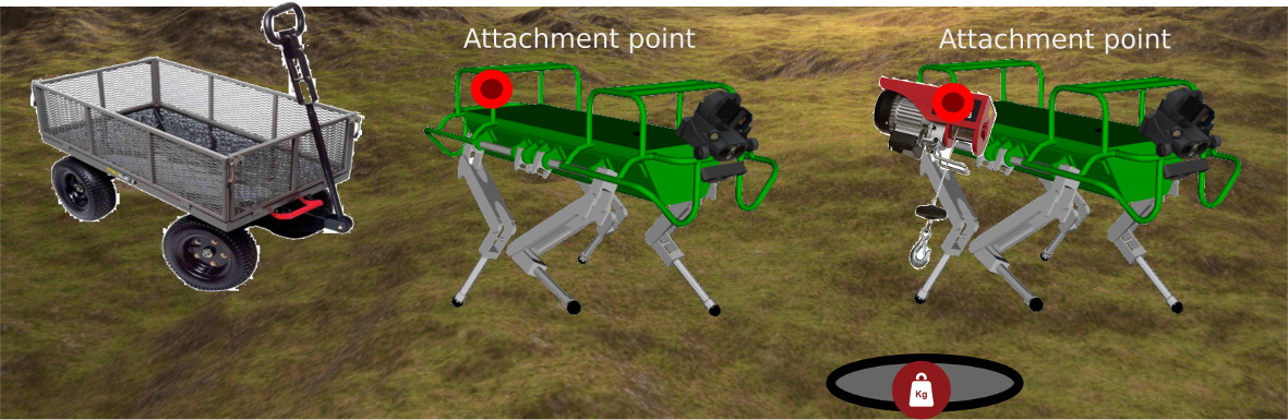
Figure 16: Use cases for load estimation: (left) the robot is pulling a cart, (right) the robot is pulling up a payload.

In this section, we present a MBDO able to estimate an external wrench (e.g. cumulative effect of all the disturbance forces and moments). We also show how this wrench is compensated during the locomotion, thus improving tracking accuracy and locomotion stability.

Our approach builds on top of the one described in [10], which is designed to estimate an external linear force acting on the robot base. We extended this work to the angular case, estimating the full wrench at the CoM.

Since our robot has a non negligible angular dynamics, estimating only a linear force has limited effectiveness. Unless the force is applied at the CoM, the application point, then the moment about the CoM must be worked out. Our approach is more general as it does not require the application point to estimate the full wrench.

The idea underlying the estimation is that any external wrench $W_{ext}\in\mathbb{R}^{6}$ has an influence on the centroidal momentum (i.e. linear and angular momentum at the CoM) [50].

We observe that the discrepancy between the predicted (centroidal) spatial momentum $\hat{h}(t)\in\mathbb{R}{{}^{6}}$, based on known forces (e.g. gravity and GRF), and the measured one $h(t)$, based on proprioceptive estimation of the CoM twist, in absence of modeling errors is caused only by an external wrench $W_{ext}$. We can exploit this fact to design an observer.

To obtain a prediction of $\hat{h}(t)=\begin{bmatrix}\hat{p}_{G}(t)&\hat{k}_{G}(t)\end{bmatrix}$, we exploit the centroidal dynamics (e.g. Newton-Euler equations)[50]:

$$\left\{\begin{array}[]{ll}\hat{\dot{p}}_{G}(t)=\underbrace{mg+\sum_{i=1}^{c}f_{i}(t)}_{f_{\text{known}}}+\hat{f}_{ext}(t)\\ \hat{\dot{k}}_{G}(t)=\underbrace{\sum_{i=1}^{c}(x_{f_{i}}(t)-x_{c}(t))\times f_{i}(t)}_{\tau_{\text{known}}}+\hat{\tau}_{ext}(t)\end{array}\right.$$ (32)

where $\hat{\dot{p}}_{G}(t)\in\mathbb{R}^{3}$ and $\hat{\dot{k}}_{G}(t)\in\mathbb{R}^{3}$ are the linear and angular momentum rate, respectively; $\hat{W}_{ext}(t)=\begin{bmatrix}\hat{f}_{ext}(t)&\hat{\tau}_{ext}(t)\end{bmatrix}$ is a prediction of the wrench disturbance at time $t$, expressed at the CoM point.

Starting from an initial measure of the momentum $h_{0}=\begin{bmatrix}p_{G0}&k_{G0}\end{bmatrix}=\begin{bmatrix}m\dot{x}_{com}(0)&I_{com}(0)\omega(0)\end{bmatrix}$, we can get the predicted $\hat{h}(t)$, at a given time $t$, by integration of Eq. (32):

$$\left\{\begin{array}[]{ll}\hat{p}_{G}(t)&=p_{0}+\int^{t}_{0}\left(mg+\sum_{i=1}^{c_{st}}f_{i}(t)+\hat{f}_{ext}(t)\right)\,dt\\ \hat{k}_{G}(t)&=k_{0}+\int^{t}_{0}(\sum_{i=1}^{c_{st}}(x_{f_{i}}(t)-x_{com}(t))\times f_{i}(t)+\\ &\quad\quad\quad\quad\quad\quad\quad\quad\quad\quad\quad\quad\quad\quad\quad\hat{\tau}_{ext}(t))\,dt\end{array}\right.$$ (33)

Then, the discrepancy between the measured and the predicted momentum can be used to estimate the external wrench disturbance, leading to the following observer set of equations:

$$\left\{\begin{array}[]{ll}\hat{f}_{ext}(t)&=G_{\text{lin}}\left(m\dot{x}_{com}(t)-\hat{p_{G}}(t)\right)\\ \hat{\tau}_{ext}(t)&=G_{\text{ang}}\left(I_{com}(t)\omega(t)-\hat{k_{G}}(t)\right)\end{array}\right.$$ (34)

where the gains $G_{\text{lin}},G_{\text{ang}}\in\mathbb{R}^{3\times 3}$ are user-defined positive definite matrices, which describe the observer’s dynamics, and $I_{com}(t)\in\mathbb{R}^{3\times 3}$ is the rotational inertia of the robot (as a rigid body) computed at time $t$. On the other hand, Eq. (32) can be rewritten using spatial algebra [49], considering the whole robot as a rigid body:

$$\dot{h}=\frac{d}{dt}(\bar{I}_{com}v)=\bar{I}_{com}\dot{v}+v\times^{\*}\bar{I}_{com}v=W_{\text{known}}+\hat{W}_{ext}$$ (35)

where $v=\begin{bmatrix}\dot{x}_{com}&\omega\end{bmatrix}\in\mathbb{R}^{6}$ is the measured CoM twist composed of CoM linear velocity and robot angular velocity (for simplicity of notation, we omit henceforth the dependency on $t$); $\bar{I}_{com}\in\mathbb{R}^{6\times 6}$ is the composite rigid body inertia (expressed in an inertial frame attached to the CoM), evaluated at each loop at the actual configuration of the robot; $W_{\text{known}}=\begin{bmatrix}f_{\text{known}}&\tau_{\text{known}}\end{bmatrix}$ is the wrench due to contacts and gravity.

Using Eq. (35), it is possible to formulate a wrench observer where the nonlinear term $v\times^{\*}\bar{I}_{com}v$ is compensated:

$$\left\{\begin{array}[]{ll}\bar{I}\hat{v}&=\bar{I}_{0}v_{0}+\int^{t}_{0}\left(W_{\text{known}}+\hat{W}_{ext}-v\times^{\*}\bar{I}_{com}v\right)\,dt\\ \hat{W}_{ext}&=G\bar{I}\left(v-\hat{v}\right)\end{array}\right.$$ (36)

where $G=\operatorname{diag}(G_{\text{lin}},G_{\text{ang}})\in\mathbb{R}^{6\times 6}$ is the observer gain matrix.

At each control loop, after the estimation step, we perform online compensation of the estimated disturbance wrench $\hat{W}_{ext}$ in the whole-body Trunk Controller [28] (see Fig. 3):

$$W^{d}=W_{vm}+W_{g}-\hat{W}_{ext}$$ (37)

where $W^{d}\in\mathbb{R}^{6}$ is the desired wrench (expressed at the CoM), mapped to desired joint torques by the Trunk Controller; $W_{g},W_{vm}\in\mathbb{R}^{6}$ are the gravity compensation wrench and the virtual model attractor (which tracks a desired CoM trajectory) wrench, respectively.

VIII-A ZMP compensation

Compensating for the external wrench is not sufficient to achieve stable locomotion. During a static crawl, the accelerations are typically small, and the ZMP mostly coincides with the projection of the CoM on the support polygon. However, this does not hold if an external disturbance is present. In this case, the ZMP can be shifted. If this is not properly accounted for in the body motion planning, the locomotion stability might be at risk.

Knowing that the ZMP is the point on the support polygon (or, better, the line) where the tangential moments nullify, the shift $\Delta x_{com}$ can be estimated by computing the equilibrium of moments about this point (see Fig. 17):

$$\underbrace{(x_{com}-x_{zmp})}_{\Delta x_{com}}\times(mg+f_{ext})+\tau_{ext}=0$$ (38)

where $\Delta x_{com}$ is the vector going from the ZMP to the CoM .

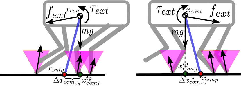
Figure 17: Diagram for the computation of the ZMP due to external disturbances. Left and right figures show different values of $\Delta x_{{com}_{xy}}$ for different external disturbances.

Rewriting Eq. (38) in an explicit form, we get [51]:

$$\left\{\begin{array}[]{ll}\Delta x_{{com}_{x}}=\frac{1}{f_{{ext}_{z}}-mg}\left[f_{{ext}_{x}}(x_{{com}_{z}}-x_{{zmp}_{z}})+\tau_{{ext}_{y}}\right]\\ \Delta x_{{com}_{y}}=\frac{1}{f_{{ext}_{z}}-mg}\left[f_{{ext}_{y}}(x_{{com}_{z}}-x_{{zmp}_{z}})-\tau_{{ext}_{x}}\right]\end{array}\right.$$ (39)

then, the new target computed at the beginning of the base motion will account for this term:

$$x_{{com}_{x,y}}^{tg}=x_{{com}_{x,y}}^{tg}+\Delta x_{{com}_{x,y}}$$ (40)

VIII-B Stability Issues

Any observer/state feedback arrangement can lead to some stability issues if the gains are not set properly (e.g. by separation principle). We did not carried out a system stability analysis, since a proper evaluation of the stability region (and an improved implementation taking care of this aspects) is an ongoing work and it is out of the scope of this paper. However, we noticed that there are some combinations of gains for which the system becomes unstable.

In the experiments, we decided to be conservative and set lower gains than in simulation. We also did not see a significant improvement in using the implementation Eq. (36) instead of Eq. (34).

VIII-C Simulations

To evaluate the quality of the estimation, we inject in simulation a known disturbance: a pure force to the back of the robot (with application point ${}_{b}x_{p}=\begin{bmatrix}-0.6,0.0,0.08\end{bmatrix}m$, expressed in the base frame), while the robot is standing still. Specifically, we generate a time-varying perturbation force $f_{ext}$ with random stepwise changes both in magnitude (between $40\text{\,}\mathrm{N}$ and $200\text{\,}\mathrm{N}$) and direction, with additive white Gaussian noise $n\in\mathcal{N}(0,20)\,$\mathrm{N}$$. The gains used in the observer are the following: $G_{ang}=\operatorname{diag}(100,100,100)$, $G_{ang}=\operatorname{diag}(10,10,10)$.

The result of the estimation is shown in Fig. 18: the estimator is able to follow promptly the step changes with the gains set, while a small filtering effect of the noise is given by the observer dynamics.

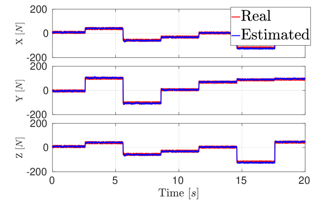
Figure 18: Simulated estimation of a time-varying external force.

To evaluate the effectiveness of the compensation, we observe that an external force not properly compensated (e.g. by the Trunk Controller) results in GRF which differ from the desired ones (outputs of the optimization), even in absence of modeling errors. This can create slippages and loss of contact, as shown in the accompanying video.

Therefore, a good metric to assess the effectiveness of the compensation is the norm of the GRF tracking error $\|f\|$.

Figure 19 shows that the compensation improves significantly the GRF tracking by almost two orders of magnitude.

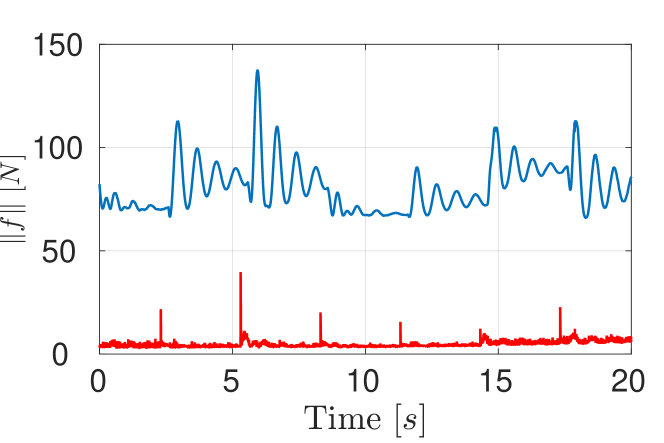
Figure 19: Norm of tracking error the with (red) and without (blue) compensation of the external wrench.

The video also shows a simulation of the robot pulling a wheelbarrow, illustrating the GRF (green arrows) and the location of the ZMP (purple sphere). In the simulation the robot “leans forward”, compensating for the offset in the ZMP created by the pulling force, while the back legs are more loaded (i.e. with larger GRF) with respect to the front ones, due to the weight of the wheelbarrow.

VIII-D Experimental Results

To demonstrate the effectiveness of our approach, we designed several test scenarios in which the robot is walking and compensating a time-varying disturbance force. In all the experiments, we set the gains to $G_{\text{lin}}=\operatorname{diag}(10,10,10),\;G_{\text{ang}}=\operatorname{diag}(1,1,1)$.

Experiment 1 - Pulling a Wheelbarrow

pulling a wheelbarrow on a ramp is an interestings experimental scenario for our MBDO.

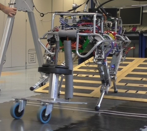
Figure 20: HyQ quadruped robot pulling a wheelbarrow (of $12\text{\,}\mathrm{kg}$) loaded with $15\text{\,}\mathrm{kg}$ of additional weight. The total vertical force acting on the robot is about $13.5\text{\,}\mathrm{kg}$. The cart is attached to the robot through a rope.

This task poses several challenges: 1) the wheelbarrow attached with a rope (intermittent unilateral pull constraint) creates a disturbance force which has a constant vertical component (to counteract wheelbarrow gravity) and a time-varying component (due to horizontal accelerations); 2) The motion of the wheel barrow results in potential unload of the rope that causes discontinuity in the force; 3) a walking gait involves a mutable contact condition, implying that the compensation force must be exerted by different legs at different times, without discontinuitiess. 4) the additional loading of the wheelbarrow is done impulsively; 5) walking on a ramp shrinks the support polygon and reduces the stability margin, requiring a high accuracy in the estimation/compensation pipeline.

The accompanying video shows the robot walking on a ramp while pulling a $12\text{\,}\mathrm{kg}$ wheelbarrow. We performed different trials, with the disturbance wrench compensation enabled, adding $10\text{\,}\mathrm{kg}$ and $5\text{\,}\mathrm{kg}$ supplementary weights (on top of the wheelbarrow), in different stages of the walk. Being the total weight of $27\text{\,}\mathrm{kg}$ equally shared between the robot and the wheels of the cart, we estimate the total load to be $13.5\text{\,}\mathrm{kg}$. With the compensation enabled, the robot is able to smoothly climb the ramp while dragging this extra weight. Without the compensation, the robot was struggling to maintain the support polygon even with $5\text{\,}\mathrm{kg}$ of extra weight (for a total load of approximately $8.5\text{\,}\mathrm{kg}$ hanging from the robot). With $15\text{\,}\mathrm{kg}$ it was unable to climb the ramp.

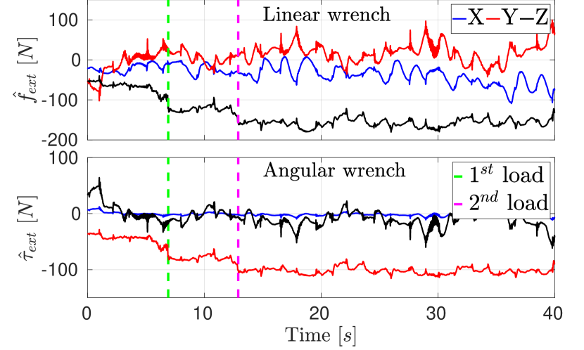
Figure 21: Wheelbarrow experiments. Estimated wrench in real experiments while the robot carries out a wheelbarrow on rough terrain, (upper plot) linear part (lower plot) the angular one. The two vertical lines represent the moments where the 1-st (10 $kg$) and 2-nd (5 $kg$) load were applied.

Figure 21 shows the components of the estimated wrench. As expected, the most relevant ones are $f_{{ext}_{x}}$, which is time varying, and $f_{{ext}_{z}}$, which is mostly the constant and vertical component of the disturbance force. Note how the vertical component $f_{{ext}_{z}}$ changes when two different loads are added to the wheelbarrow. The wheelbarrow is attached to the back of the robot, hence it also exerts a constant negative moment around the $Y$ direction.

Since the interaction force with the wheelbarrow is unknown, again the GRF tracking is the only metric available to assess the quality of the compensation. Figure 22 shows the pitch variation (upper plot) while walking first horizontally and then up the slope. The GRF tracking for the $LH$ leg is also shown (lower plot). Thanks to the compensation, the tracking error is always below $40\text{\,}\mathrm{N}$ for the Z component (about $5\text{\,}\mathrm{\char 37\relax}$ of the total robot’s weight) and $20\text{\,}\mathrm{N}$ for the X component.

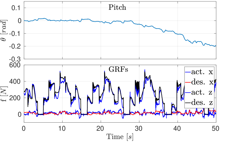
Figure 22: Wheelbarrow experiments: (upper plot) trunk pitch angle and (lower plot) tracking of the $Z$ component of the GRF of the $LH$ leg, while the robot carries the wheelbarrow on ramp.

Experiment 2 - Leaning Against a Pulling Force

In this experiment, a $15\text{\,}\mathrm{kg}$ load is attached to the back of the robot with a rope. An intermediate pulley transforms the gravitational load into a horizontal force. This test allows to evaluate the effectiveness of the estimation/compensation pipeline in presence of disturbance forces mostly horizontal.

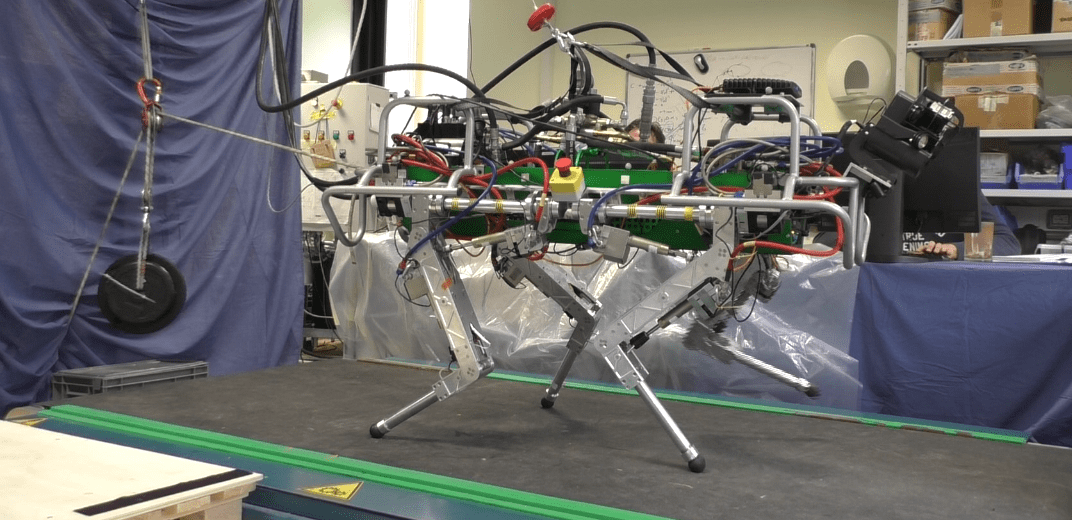
Figure 23: HyQ quadruped robot dragging a $75N$ horizontal disturbance force (15 $kg$ load on a pulley) to testing the performances of the MBDO.

In the experiments, the robot is able to pull $15\text{\,}\mathrm{kg}$ when walking with the compensation enabled. When the estimation is disabled, the controller accumulates errors and suffers from instability. Figure 24 shows that the only significant component in the estimated wrench is along the $X$ direction (horizontal). The force increases, while the robot walks, because the load is pulled up gradually (see video), until it reaches the steady value of $75\text{\,}\mathrm{N}$ (i.e. the $15\text{\,}\mathrm{kg}$ load halved by the pulley

).

Figure 24: Curling experiments. Estimated wrench: (upper plot) linear part, the load is mainly along the $X$ component (horizontal) (lower plot) angular part, all the moments are oscillating around zero, showing that the interaction force direction is passing close to the CoM.

The RViz visualization in the accompanying video shows that the GRF have a constant component along the $X$ direction (e.g. pointing forward) to compensate for the backward pulling force. At the same time, when the compensation is active, the ZMP is shifted forward.

IX Conclusions

In this work we addressed the problem of locomotion on rough terrain. We proposed a 1-step receeding horizon heuristic planning strategy that can work with variable levels of exteroceptive feedbacks.

When no exteroceptive perception is available (and no map of the environment is given to the robot) the locomotion framework presented in this paper is still capable of traversing challenging terrains. This is possible thanks to its capability to blindly adapt to the terrain, mainly because of the 1-step re-planning and of the haptic touchdown.

When a map of the surrounding world is available, the proposed locomotion framework can exploit this information by including the actual terrain height and orientation in the planning, thus decreasing the chances of stumbling and allowing to traverse more difficult situations (e.g. climbing stairs).

With the proposed approach we were able to achieve several experimental results, such as traversing a template rough terrain made of ramps, debris and stairs. We have also shown our quadruped walking while compensating for external time-varying disturbance forces caused by a load up to $15\text{\,}\mathrm{kg}$, using the MBDO that we proposed. All these tasks where performed with the same locomotion strategy that we presented in this paper.
Future works involve an extensive analysis of the stability of the MBDO, considering its interactions with the Trunk Controller loop. Based on these results, we intend to implement improved observer that maximizes the stability region. Our future research directions also include extending the navigation capabilities of HyQ to more complex environments made of rolling stones and big size obstacles ($>$$12\text{\,}\mathrm{cm}$ diameter). For these scenarios, we envision the need to develop a shin collision detection algorithm capable of kino-dynamic proprioception using a foot-switch sensor[34]. Finally, we plan to carry out extensive stair climbing experiments with the proposed approach.

Appendix A

This appendix shows how to compute the weighted average of $N$ orientation vectors.

Because finite rotations do not sum up as vectors do, it is not possible to apply ordinary laws of vector arithmetic to them. Specifically, the task of averaging orientations (described in the algorithm 1 written in pseudo-code) is equivalent to average points on a sphere, where the line is replaced with a spherical geodesic (arc of a circle).

Algorithm 1 compute geodesic average

1:$w_{1}\leftarrow 1$

2:$\bar{n}\leftarrow n_{1}$

3:for $k=2$ to $N$ do

4:     $\theta_{k}=acos(\text{dot}(\bar{n},n_{k}))$

5:     $\bar{\theta}_{k}=\theta_{k}\frac{\sum\limits_{p=1}^{k-1}w_{p}}{\sum\limits_{p=1}^{k}w_{p}}$

6:     $\bar{n}\leftarrow$ rotate $n_{k}$ towards $\bar{n}$ by angle $\bar{\theta}_{k}$

7:end for

The iterative procedure illustrated above is generic and can be used to obtain the average of $N$ directional vectors $n_{k}$, even though at each iteration we are only able to directly compute the average of two. After the initialization, at each loop the actual average $\bar{n}$ is updated with the next normal $n_{k}$. To do so, we first compute the angle $\theta_{k}$ between $n_{k}$ and the actual average $\bar{n}$. Then we scale this angle, according to the (accumulated) weight of $\bar{n}$. Finally, $n_{k}$ is rotated by the scaled angle $\hat{\theta}$ toward $\bar{n}$ and the result is assigned back to $\bar{n}$.

Appendix B

List of the main symbols used throughout the paper:
Symbol Description $x_{com}\in\mathbb{R}^{3}$ coordinates of the CoM of the robot $x_{fi},\dot{x}_{fi}\in\mathbb{R}^{3}$ positions and velocities of the $i^{th}$ foot $f_{i}\in\mathbb{R}^{3}$ contact forces of the $i^{th}$ stance foot $n$ number of active joints of the robot $q^{d}_{j},\dot{q}^{d}_{j}\in\mathbb{R}^{n}$ joint reference positions and velocities $\tau_{ff}^{d}\in\mathbb{R}^{n}$ feedforward torque command $\tau_{pd}^{d}\in\mathbb{R}^{n}$ impedance torque command $\tau^{d}\in\mathbb{R}^{n}$ total reference torque command $\phi$ roll angle of the robot’s trunk $\theta$ pitch angle of the robot’s trunk $\psi$ yaw angle of the robot’s trunk $\Phi=[\phi,\theta,\psi]$ actual orient. of the robot’s trunk $\Phi^{d}=[\phi^{d},\theta^{d},\psi^{d}]$ desired orient. of the robot’s trunk $\Phi^{d}(0)=\Phi$ des. orient. at the start of the move base $\Phi^{tg}$ target orient. at the end of the move base $x_{com}^{tg}$ target CoM position of the trunk $x_{{com}_{p}}^{tg}$ projection of $x_{com}^{tg}$ on the terrain plane $h_{r}$ robot’s height $f_{ext},\tau_{ext}$ external disturbance force and torque

References

- [1] T. Bretl and S. Lall, “Testing static equilibrium for legged robots,” IEEE Transactions on Robotics, vol. 24, pp. 794–807, Aug 2008.
- [2] D. Pardo, L. Möller, M. Neunert, A. W. Winkler, and J. Buchli, “Evaluating Direct Transcription and Nonlinear Optimization Methods for Robot Motion Planning,” IEEE Robotics and Automation Letters, vol. 1, no. 2, pp. 946–953, 2016.
- [3] C. Mastalli, M. Focchi, I. Havoutis, A. Radulescu, S. Calinon, J. Buchli, D. G. Caldwell, and C. Semini, “Trajectory and foothold optimization using low-dimensional models for rough terrain locomotion,” in IEEE International Conference on Robotics and Automation (ICRA), 2017.
- [4] A. W. Winkler, C. D. Bellicoso, M. Hutter, and J. Buchli, “Gait and Trajectory Optimization for Legged Systems through Phase-based End-Effector Parameterization,” IEEE Robotics and Automation Letters, pp. 1–1, 2018.
- [5] B. Aceituno-Cabezas, C. Mastalli, D. Hongkai, M. Focchi, A. Radulescu, D. G. Caldwell, J. Cappelletto, J. C. Grieco, G. Fernando-Lopez, and C. Semini, “Simultaneous Contact, Gait and Motion Planning for Robust Multi-Legged Locomotion via Mixed-Integer Convex Optimization,” IEEE Robotics and Automation Letters, pp. 1–8, 2018.
- [6] C. Mastalli, A. W. Winkler, I. Havoutis, D. G. Caldwell, and C. Semini, “On-line and On-board Planning and Perception for Quadrupedal Locomotion,” in IEEE International Conference on Technologies for Practical Robot Applications (TEPRA), 2015.
- [7] H. Dai and R. Tedrake, “Planning robust walking motion on uneven terrain via convex optimization,” 2016 IEEE-RAS International Conference on Humanoid Robots (Humanoids 2016), 2016.
- [8] B. Ponton, A. Herzog, A. Del Prete, S. Schaal, and L. Righetti, “On Time Optimisation of Centroidal Momentum Dynamics,” https://arxiv.org/abs/1709.09265, 2017.
- [9] B. J. Stephens, “State estimation for force-controlled humanoid balance using simple models in the presence of modeling error,” in 2011 IEEE International Conference on Robotics and Automation, pp. 3994–3999, May 2011.
- [10] J. Englsberger, G. Mesesan, and C. Ott, “Smooth trajectory generation and push-recovery based on divergent component of motion,” in IEEE International Conference on Intelligent Robots and Systems (IROS), pp. 4560–4567, September 2017.
- [11] N. Rotella, “Estimation-based control for humanoid robots,” in PhD Thesis, University of Southern California (USC), 2018.
- [12] G. Bledt, P. M. Wensing, and S. Kim, “Policy-regularized model predictive control to stabilize diverse quadrupedal gaits for the MIT cheetah,” IEEE/RSJ International Conference on Intelligent Robots and Systems (IROS), pp. 4102–4109, 2017.
- [13] P.-B. Wieber, “Trajectory Free Linear Model Predictive Control for Stable Walking in the Presence of Strong Perturbations Trajectory Free Linear Model Predictive Control for Stable Walking in the Presence of Strong Perturbations,” IEEE-RAS International Conference on Humanoid Robots, 2006.
- [14] H.-W. Park, P. Wensing, and S. Kim, “Online Planning for Autonomous Running Jumps Over Obstacles in High-Speed Quadrupeds,” Robotics: Science and Systems XI, 2015.
- [15] C. D. Bellicoso, C. Gehring, J. Hwangbo, P. Fankhauser, and M. Hutter, “Perception-less terrain adaptation through whole body control and hierarchical optimization,” in 2016 IEEE-RAS 16th International Conference on Humanoid Robots (Humanoids), pp. 558–564, Nov 2016.
- [16] C. D. Bellicoso, F. Jenelten, P. Fankhauser, C. Gehring, J. Hwangbo, and M. Hutter, “Dynamic Locomotion and Whole-Body Control for Quadrupedal Robots,” IEEE/RSJ Intenational Conference on Intelligent Robots and Systems (IROS), pp. 3359–3365, 2017.
- [17] P. Fankhauser, M. Bjelonic, C. D. Bellicoso, T. Miki, and M. Hutter, “Robust rough-terrain locomotion with a quadrupedal robot,” IEEE International Conference on Robotics and Automation (ICRA), 2018.
- [18] M. Fallon, P. Marion, R. Deits, T. Whelan, M. Antone, J. McDonald, and R. Tedrake, “Continuous humanoid locomotion over uneven terrain using stereo fusion,” in 2015 IEEE-RAS 15th International Conference on Humanoid Robots (Humanoids), pp. 881–888, nov 2015.
- [19] M. Camurri, M. Fallon, S. Bazeille, A. Radulescu, V. Barasuol, D. G. Caldwell, and C. Semini, “Probabilistic Contact Estimation and Impact Detection for State Estimation of Quadruped Robots,” IEEE Robotics and Automation Letters, vol. 2, pp. 1023–1030, apr 2017.
- [20] M. Bloesch, M. Hutter, M. H. Hoepflinger, C. Gehring, C. David Remy, and R. Siegwart, “State estimation for legged robots: Consistent fusion of leg kinematics and IMU,” vol. 8, pp. 17–24, MIT Press Journals, 2013.
- [21] X. Xinjilefu, S. Feng, W. Huang, and C. G. Atkeson, “Decoupled state estimation for humanoids using full-body dynamics,” in 2014 IEEE International Conference on Robotics and Automation (ICRA), pp. 195–201, May 2014.
- [22] S. Nobili, M. Camurri, V. Barasuol, M. Focchi, D. Caldwell, C. Semini, and M. Fallon, “Heterogeneous Sensor Fusion for Accurate State Estimation of Dynamic Legged Robots,” Robotics: Science and Systems XIII, 2017.
- [23] V. Barasuol, J. Buchli, C. Semini, M. Frigerio, E. R. De Pieri, and D. G. Caldwell, “A reactive controller framework for quadrupedal locomotion on challenging terrain,” Proceedings - IEEE International Conference on Robotics and Automation, pp. 2554–2561, 2013.
- [24] M. Focchi, V. Barasuol, M. Frigerio, D. G. Caldwell, and C. Semini, “Slip Detection and Recovery for Quadruped Robots,” vol. 3, pp. 185–199, Cham: Springer Proceedings in Advanced Robotics, 2018.
- [25] V. Barasuol, M. Camurri, S. Bazeille, D. Caldwell, and C. Semini, “Reactive trotting with foot placement corrections through visual pattern classification,” in IEEE/RSJ International Conference on Intelligent Robots and Systems (IROS), 10 2015.
- [26] D. Belter and P. Skrzypczyński, “Rough terrain mapping and classification for foothold selection in a walking robot,” Journal of Field Robotics, vol. 28, no. 4, pp. 497–528, 2011.
- [27] C. Mastalli, I. Havoutis, M. Focchi, D. G. Caldwell, and C. Semini, “Motion planning for quadrupedal locomotion: coupled planning, terrain mapping and whole-body control,” HAL id: hal-01673438v2, 2018.
- [28] M. Focchi, A. Del Prete, I. Havoutis, R. Featherstone, D. G. Caldwell, and C. Semini, “High-slope terrain locomotion for torque-controlled quadruped robots,” Autonomous Robots, vol. 41, no. 1, pp. 259–272, 2017.
- [29] M. Focchi, R. Featherstone, R. Orsolino, D. G. Caldwell, and C. Semini, “Viscosity-based height reflex for workspace augmentation for quadrupedal locomotion on rough terrain,” in IEEE/RSJ International Conference on Intelligent Robots and Systems (IROS), 2017.
- [30] M. Focchi, V. Barasuol, I. Havoutis, J. Buchli, C. Semini, and D. G. Caldwell, “Local reflex generation for obstacle negotiation in quadrupedal locomotion,” in Int. Conf. on Climbing and Walking Robots (CLAWAR), 2013.
- [31] C. Semini, N. Tsagarakis, E. Guglielmino, M. Focchi, F. Cannella, and D. Caldwell, “Design of HyQ – a Hydraulically and Electrically Actuated Quadruped Robot,” J. of Systems and Control Eng., 2011.
- [32] M. Frigerio, J. Buchli, D. G. Caldwell, and C. Semini, “RobCoGen: a code generator for efficient kinematics and dynamics of articulated robots, based on Domain Specific Languages,” vol. 7, no. 1, pp. 36–54, 2016.
- [33] A. S. Tar, G. G. Cserey, and J. Veres, May 2014. Patent N. WO 2013072712 A1.
- [34] Y. Gao, C. Semini, M. Focchi, and D. G. Caldwell, February 2018. Patent N. IT 102018000002407.
- [35] A. Winkler, C. Mastalli, I. Havoutis, M. Focchi, D. G. Caldwell, and C. Semini, “Planning and execution of dynamic whole-body locomotion for a hydraulic quadruped on challenging terrain,” in IEEE International Conference on Robotics and Automation (ICRA), May 2015.
- [36] T. Boaventura, J. Buchli, C. Semini, and D. G. Caldwell, “Model-based hydraulic impedance control for dynamic robots,” IEEE Transactions on Robotics, vol. 31, pp. 1324–1336, Dec 2015.
- [37] R. Orsolino, M. Focchi, C. Mastalli, H. Dai, D. G. Caldwell, and C. Semini, “Application of Wrench based Feasibility Analysis to the Online Trajectory Optimization of Legged Robots,” IEEE Robotics and Automation Letters (RA-L), 2018.
- [38] H. Audren and A. Kheddar, “3D robust stability polyhedron in multi-contact,” Submitted to IEEE Transactions On Robotics (TRO), 2017.
- [39] R. M. Alexander, Principles of animal locomotion. Princeton University Press, 2003.
- [40] C. Semini, N. G. Tsagarakis, E. Guglielmino, M. Focchi, F. Cannella, and D. G. Caldwell, “Design of hyq - a hydraulically and electrically actuated quadruped robot,” IMechE Part I: Journal of Systems and Control Engineering, vol. 225, no. 6, pp. 831–849, 2011.
- [41] M. Camurri, Multisensory State Estimation and Mapping on Dynamic Quadruperd Robots. PhD thesis, Istituto Italiano di Tecnologia (IIT) and Universiy of Genoa, 2017. http://iit-dlslab.github.io/papers/camurri17phd.pdf.
- [42] P. Fankhauser and M. Hutter, “A Universal Grid Map Library: Implementation and Use Case for Rough Terrain Navigation,” in Robot Operating System (ROS) – The Complete Reference (Volume 1) (A. Koubaa, ed.), ch. 5, Springer, 2016.
- [43] C. Semini, V. Barasuol, J. Goldsmith, M. Frigerio, M. Focchi, Y. Gao, and D. G. Caldwell, “Design of the hydraulically-actuated, torque-controlled quadruped robot hyq2max,” IEEE/ASME Transactions on Mechatronics, vol. PP, no. 99, pp. 1–1, 2016.
- [44] C. Gramkow, “On averaging rotations,” Journal of Mathematical Imaging and Vision, vol. 15, no. 1-2, pp. 7–16, 2001.
- [45] C. Gehring, S. Coros, M. Hutler, C. Dario Bellicoso, H. Heijnen, R. Diethelm, M. Bloesch, P. Fankhauser, J. Hwangbo, M. Hoepflinger, and R. Siegwart, “Practice Makes Perfect: An Optimization-Based Approach to Controlling Agile Motions for a Quadruped Robot,” IEEE Robotics and Automation Magazine, vol. 23, no. 1, pp. 34–43, 2016.
- [46] S. Oßwald, J. S. Gutmann, A. Hornung, and M. Bennewitz, “From 3d point clouds to climbing stairs: A comparison of plane segmentation approaches for humanoids,” in 2011 11th IEEE-RAS International Conference on Humanoid Robots, pp. 93–98, Oct 2011.
- [47] D. Pongas, M. Mistry, and S. Schaal, “A Robust Quadruped Walking Gait for Traversing Rough Terrain,” in Proceedings 2007 IEEE International Conference on Robotics and Automation, pp. 1474–1479, April 2007.
- [48] G. Tournois, M. Focchi, A. Del Prete, R. Orsolino, D. G. Caldwell, and C. Semini, “Online payload identification for quadruped robots,” in IEEE/RSJ International Conference on Intelligent Robots and Systems (IROS), 2017.
- [49] R. Featherstone, “Rigid Body Dynamics Algorithms,” Springer US, Boston, MA, 2008.
- [50] D. E. Orin, A. Goswami, and S.-H. Lee, “Centroidal dynamics of a humanoid robot,” Autonomous Robots, vol. 35, pp. 161–176, Oct 2013.
- [51] M. B. Popovic, A. Goswami, and H. Herr, “Ground reference points in legged locomotion: Definitions, biological trajectories and control implications,” The International Journal of Robotics Research, vol. 24, no. 12, pp. 1013–1032, 2005.