subsecref subsecname = thmref thmname = theorem  lemref lemname = lemma  caprefcmd=Figure LABEL:#1 figrefcmd=Figure LABEL:#1 tabrefcmd=Table LABEL:#1 secrefcmd=Section LABEL:#1 subsecrefcmd=Section LABEL:#1 eqrefcmd=Equation LABEL:#1

Reconciliation of weak pairwise spike-train correlations and highly
coherent local field potentials across space

Johanna Senk^1*, Espen Hagen^1,2, Sacha J. van Albada^1,3, Markus Diesmann^1,4,5

¹Institute of Neuroscience and Medicine (INM-6) and Institute for Advanced Simulation (IAS-6) and JARA Institute Brain Structure-Function Relationships (INM-10), Jülich Research Centre, 52428 Jülich, Germany

²NORMENT Centre, Institute of Clinical Medicine, University of Oslo, and Division of Mental Health and Addiction, Oslo University Hospital, 0424 Oslo, Norway

³Institute of Zoology, University of Cologne, 50674 Cologne, Germany

⁴Department of Psychiatry, Psychotherapy and Psychosomatics, Medical Faculty, RWTH Aachen University, 52074 Aachen, Germany

⁵Department of Physics, Faculty 1, RWTH Aachen University, 52074 Aachen, Germany

^*j.senk@fz-juelich.de

Conflict of Interest

The authors declare no competing financial interests.

Abstract

Multi-electrode arrays covering several square millimeters of neural tissue provide simultaneous access to population signals such as extracellular potentials and spiking activity of one hundred or more individual neurons. The interpretation of the recorded data calls for multiscale computational models with corresponding spatial dimensions and signal predictions. Such models facilitate identifying candidate mechanisms underlying experimentally observed spatiotemporal activity patterns in the cortex. Multi-layer spiking neuron network models of local cortical circuits covering about $1\,\mathrm{mm^{2}}$ have been developed, integrating experimentally obtained neuron-type-specific connectivity data and reproducing features of observed in-vivo spiking statistics. Local field potentials (LFPs) can be computed from the simulated spiking activity. We here extend a local network and LFP model to an area of $4\times 4\,\mathrm{mm^{2}}$. The upscaling preserves the densities of neurons while capturing a larger proportion of the local synapses within the model. The procedure further introduces distance-dependent connection probabilities and conduction delays. Based on model predictions of spiking activity and LFPs, we find that the upscaling procedure preserves the overall spiking statistics of the original model and reproduces asynchronous irregular spiking across populations and weak pairwise spike-train correlations in agreement with experimental data recorded in the sensory cortex. In contrast with the weak spike-train correlations, the correlation of LFP signals is strong and decays over a distance of several hundred micrometers, compatible with experimental observations. Enhanced spatial coherence in the low-gamma band around $50\,\mathrm{Hz}$ may explain the recent experimental report of an apparent band-pass filter effect in the spatial reach of the LFP.

Significance Statement

Extracellular recordings with multi-electrode arrays measure both population signals such as the local field potential (LFP) and spiking activity of individual neurons across the cortical tissue, for instance covering the $4\times 4\,\mathrm{mm^{2}}$ of a Utah array. To reproduce key features of activity data obtained from such cortical patches, we assess spiking activity and LFPs of a multiscale neuronal network model of this spatial extent. The circuit incorporates biological details such as a realistic neuron density across four cortical layers and neuron-type-specific, layer-specific, and distance-dependent connectivity. The model reconciles experimental observations like a frequency-dependent LFP coherence across space with weak pairwise spike-train correlations.

1 Introduction

Cortical activity on the mesoscopic scale (mesoscale – spanning several millimeters to centimeters; Muller et al., 2018), can be recorded with implanted multi-electrode arrays (Maynard et al., 1997; Buzsáki et al., 2012). The local field potential (LFP) is the low-frequency part ($\lesssim 500\,\mathrm{Hz}$) of the measured extracellular signal, primarily reflecting synaptic activations (Einevoll et al., 2013a) across millions of local and distant neurons (Kajikawa and Schroeder, 2011; Lindén et al., 2011; Łęski et al., 2013). Spike sorting (Quiroga, 2007) extracts spikes of individual neurons from the high-frequency part ($\gtrsim 100\,\mathrm{Hz}$) of the signal. From Utah array recordings ($10\times 10$ electrodes on $4\times 4\,\mathrm{mm^{2}}$, Blackrock Neurotech, https://blackrockneurotech.com) one may identify spiking activity of $\mathcal{{O}}\left(100\right)$ neurons (Riehle et al., 2013). Such recordings also expose propagating LFP activity associated with distance dependence of statistical measures like correlations and coherences (Destexhe et al., 1999; Smith and Kohn, 2008; Wu et al., 2008; Dubey and Ray, 2016), contrasting the low pairwise correlation in cortical spike trains characteristic of asynchronous brain states (e.g., Ecker et al., 2010).

Assuming a neuron density of $\mathcal{{O}}\left(10^{5}\right)\,\mathrm{neurons/mm^{2}}$ across the human cortical surface (Herculano-Houzel, 2009), a Utah array covers over a million neurons. Every neuron receives up to ${O}\left(10^{4}\right)$ synapses from both nearby and distant neurons (Abeles, 1991; Sherwood et al., 2020), forming local circuits specific to cortical layers and neuron types (Douglas et al., 1989; Thomson et al., 2002; Binzegger et al., 2004; Korcsak-Gorzo et al., 2022). Most local cortical connections onto postsynaptic neurons occur within $\lesssim 500\,\mathrm{\mu m}$ from presynaptic neurons (Voges et al., 2010), with connection probabilities decaying approximately exponentially with distance (Perin et al., 2011). Local intracortical connections are typically made by unmyelinated axons, leading to conduction delays governed by axonal propagation speeds of around $0.3\,\mathrm{mm/ms}$ (Hirsch and Gilbert, 1991), which is in line with mesoscopic wave propagation speeds (Sato et al., 2012; Denker et al., 2018; Muller et al., 2018).

The relationship between cortical connectivity and experimentally recorded spikes and LFPs at the mesoscale remains poorly understood. Network models encompassing the relevant anatomical and physiological detail, spatial scales, and corresponding measurements can aid the interpretation of experimental observations. We advocate for full-scale models with realistic neuron and synapse counts: Downscaled or diluted models may not reproduce first- and second-order statistics of full-scale networks (van Albada et al., 2015). Hagen et al. (2016) demonstrate that biophysics-based predictions of LFP signals also require the full density of cells and connections to account for network correlations. The microcircuit model by Potjans and Diesmann (2014) is a full-density model of a $1\,\mathrm{mm^{2}}$ patch of early sensory cortex with neuron-type- and layer-specific connection probabilities derived from anatomical and electrophysiological data. This model produces biologically plausible firing rates across four cortical layers with one excitatory and inhibitory population per layer, permits rigorous mathematical analysis, is freely available, and is actively used by the community in neuroscientific studies (e.g., Wagatsuma et al., 2011; Cain et al., 2016; Schwalger et al., 2017; Schmidt et al., 2018a) and as a benchmark model for neuromorphic computing (e.g., van Albada et al., 2018; Kauth et al., 2023).

Here, we upscale a version of this microcircuit model (adapted to area V1 of macaque cortex by Schmidt et al., 2018a) to the cortical surface covered by Utah arrays, introducing distance-dependent connectivity and corresponding LFP measurements. We hypothesize that this upscaled model not only preserves original activity features but also elucidates mesoscale phenomena such as the spatial propagation of evoked neuronal activity (Bringuier et al., 1999; Muller et al., 2014) and strong distance-dependent correlations and coherences in the measured LFP (Destexhe et al., 1999; Katzner et al., 2009; Nauhaus et al., 2009; Kajikawa and Schroeder, 2011; Jia et al., 2011; Srinath and Ray, 2014; Dubey and Ray, 2016), even for network states with weak pairwise spike-train correlations (e.g., Ecker et al., 2010; Dahmen et al., 2022).

2 Materials and Methods

2.1 Point-neuron networks

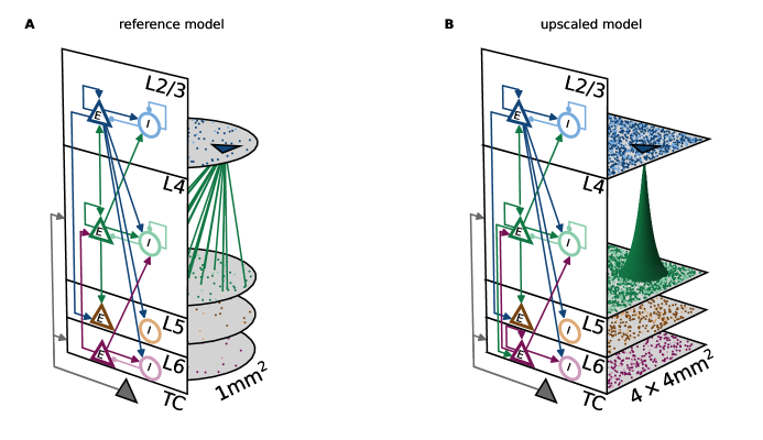
Figure 1: Comparison of point-neuron network models. A Reference model ($1\,\mathrm{mm^{2}}$ cortical microcircuit without spatial organization, adapted from the model introduced by Potjans and Diesmann, 2014 to macaque V1 by Schmidt et al., 2018a). B Upscaled model ($4\times 4\,\mathrm{mm^{2}}$ in two-dimensional layers with spatial organization). Both models represent four cortical layers ($\mathrm{L2/3}$, $\mathrm{L4}$, $\mathrm{L5}$, $\mathrm{L6}$) with an excitatory ($\mathrm{E}$) and an inhibitory ($\mathrm{I}$) population each, and an external thalamic population ($\mathrm{TC}$). The 2D network sketches illustrate by arrows the main population-specific projections (average in-degree larger than $300$). The 3D representation exemplifies connections from $\mathrm{L4E}$ to a target neuron in $\mathrm{L2/3E}$ (no spatial dependence in reference model, exponential local connectivity profile in upscaled model). Layer thicknesses in the sketches are proportional to the neuron numbers per layer; cell bodies (dots) projected to bottom of layer to indicate that cortical depth within layer has no relevance for model.

The reference model (illustrated in 1A, parameters with superscript $\mathrm{r}$) is extended to the larger upscaled model (illustrated in 1B, parameters with superscript $\mathrm{u}$) by spatial structure. Tables 1 and 2 provide the full network descriptions. Each model represents a part of early sensory cortex at full neuron and synapse density. The eight neuron populations within each network are organized into four cortical layers, that is, layer $2/3$ ($\mathrm{L2/3}$), layer $4$ ($\mathrm{L4}$), layer $5$ ($\mathrm{L5}$) and layer $6$ ($\mathrm{L6}$). Each layer contains an excitatory ($\mathrm{E}$) and an inhibitory ($\mathrm{I}$) population of leaky integrate-and-fire (LIF) model neurons, whose sub-threshold membrane dynamics are governed by (LABEL:lif_subthreshold).

The probabilities for two neurons to be connected are specific to the combination of source and target population and derived from a number of anatomical and electrophysiological studies (Potjans and Diesmann, 2014). The reference model is further refined to area V1 of macaque cortex using the parameterization of the multi-area model proposed by Schmidt et al. (2018a, b). Postsynaptic currents have static, normally distributed amplitudes and decay exponentially (Equations 15 and 16). All neurons receive stationary external input in the form of Poisson spike trains with a fixed rate; this input here also compensates for missing connections from other areas of the multi-area model. In addition, one population of thalamocortical ($\mathrm{TC}$) neurons targeting $\mathrm{E}$ and $\mathrm{I}$ neurons in both $\mathrm{L4}$ and $\mathrm{L6}$ can provide further external input, for example to emulate stimuli of the sensory pathway. We refer to the total set of populations as $X_{\mathrm{total}}=X_{\mathrm{E}}\cup X_{\mathrm{I}}$, where $X_{\mathrm{E}}=\left\{\mathrm{L2/3,L4,L5,L6}\right\}\times\mathrm{\left\{E\right\}}\cup\mathrm{\left\{TC\right\}}$ is the subset of excitatory populations and $X_{\mathrm{I}}=\left\{\mathrm{L2/3,L4,L5,L6}\right\}\times\mathrm{\left\{I\right\}}$ is the subset of inhibitory populations, respectively. The connectivity is defined via projections from a presynaptic population $X\in X_{\mathrm{total}}$ to a postsynaptic population $Y\in X_{\mathrm{total}}\backslash\left\{\mathrm{TC}\right\}$. Thus, we use the distinction between connections (i.e., atomic edges between individual network nodes) and projections (i.e., collections of connections) introduced by Senk et al. (2022).

Both network models are available as executable descriptions in the language consumed by the simulation code NEST (http://www.nest-simulator.org, Gewaltig and Diesmann, 2007). Upon execution, the simulation engine instantiates a realization of the models in the main memory of the computer based on the statistical descriptions of network connectivity. The model specifications are set up such that the same code is used for both the reference and the upscaled model, but with different parameters. The code to reproduce the simulations is publicly available on GitHub (https://github.com/INM-6/mesocircuit-model).

The following explains how the upscaled model is derived from the reference model, highlights the differences between the two, and provides a justification for choices of parameter values (Tables 3 and 4).

2.1.1 Neuron numbers and space

In the reference model, each population $X$ is composed of $N_{X}^{\mathrm{r}}$ neurons. This model represents the cortical tissue below a surface area of $A^{\mathrm{r}}=1\,\mathrm{mm^{2}}$ but neurons are not assigned spatial coordinates.

The upscaled model assigns spatial coordinates to neurons in two dimensions. Neuron positions are drawn randomly from a uniform distribution within a square domain of side length $L=4\,\mathrm{mm}$ with the origin $\left(0,0\right)$ at the center. The area covered by the model is therefore $A^{\mathrm{u}}=L^{2}$. The neuron densities per square millimeter of the reference model are preserved, so the size of a population $X$ in the upscaled model is

$$N_{X}^{\mathrm{u}}=N_{X}^{\mathrm{r}}\frac{A^{\mathrm{u}}}{A^{\mathrm{r}}}.$$ (1)

The reference model comprises $198,834$ neurons and $388,515,188$ synapses under $1\,\mathrm{mm^{2}}$ of cortical surface area, while the upscaled model consists of $3,181,344$ neurons and $7,661,094,874$ synapses and covers an area of $4\times 4\,\mathrm{mm^{2}}$, similar to the area covered by the Utah multi-electrode array.

2.1.2 Synaptic time constants and strengths

The reference model uses the same synaptic time constant $\tau_{\mathrm{s}}^{\mathrm{r}}$ for all projections. Synaptic strengths in this model are proportional to synaptic strength $J$ with a projection-specific factor $g_{YX}^{\mathrm{r}}$ for projections from population $X$ to population $Y$. The upscaled model uses different synaptic time constants for excitatory and inhibitory projections: $\tau_{\mathrm{s,E}}^{\mathrm{u}}$ and $\tau_{\mathrm{s,I}}^{\mathrm{u}}$, respectively. To preserve the total charge, i.e., the integral of a postsynaptic current due to a presynaptic spike, we compensate synaptic weights by adjusting the relative synaptic strengths:

$$g_{YX}^{\mathrm{u}}=g_{YX}^{\mathrm{r}}\cdot\begin{cases}\tau_{\mathrm{s}}^{\mathrm{r}}/\tau_{\mathrm{s,E}}^{\mathrm{u}}&\text{if }X\in X_{\mathrm{E}}\\ \tau_{\mathrm{s}}^{\mathrm{r}}/\tau_{\mathrm{s,I}}^{\mathrm{u}}&\text{if }X\in X_{\mathrm{I}}.\end{cases}$$ (2)

Note that the default factor for inhibitory projections is $g_{Y\mathrm{X}}^{\mathrm{r}}=11$ for $X\in X_{\mathrm{I}}$ as in the model by Schmidt et al. (2018a) instead of $4$ as in the original model by Potjans and Diesmann (2014). Inhibitory postsynaptic potential amplitudes tend to be larger than excitatory ones, but a factor of $11$ is most likely overestimated (Avermann et al., 2012). However, here we follow the model of Schmidt et al. (2018a) to obtain a plausible dynamical state in the reference model.

In the upscaled model, the time constants of postsynaptic currents are $\tau_{\mathrm{s,E}}^{\mathrm{u}}=2\,\mathrm{ms}$ and $\tau_{\mathrm{s,I}}^{\mathrm{u}}=8\,\mathrm{ms}$ for excitatory and inhibitory projections, respectively, versus $\tau_{\mathrm{s}}^{\mathrm{r}}=0.5\,\mathrm{ms}$ used for all synapses in the reference model. This change between the reference and upscaled model accounts for the observed differences in decay time constants of AMPA and GABA_A synaptic conductances. The $\tau_{\mathrm{s,E}}^{\mathrm{u}}$ and $\tau_{\mathrm{s,I}}^{\mathrm{u}}$ values are inferred from synaptic conductance decay time constants used in the model by Markram et al. (2015), via model files available on the the Neocortical Microcircuit Collaboration Portal (Ramaswamy et al., 2015). We ignored the short rise time constants. Synaptic NMDA currents with very long time constants are not accounted for. The adjustment of the synaptic strengths to preserve the total electric charge delivered by the postsynaptic currents in the reference model ((LABEL:relative_synaptic_strength)) reduces the relative strength of inhibition to a factor of $-2.75$ compared to the factor of $-11$ in the reference model.

2.1.3 Connectivity

In the reference model, a neuron $j$ in a source population $X$ of size $N_{X}^{\mathrm{r}}$ connects at random to a neuron $i$ in a target population $Y$ of size $N_{Y}^{\mathrm{r}}$ with mean connection probability (Potjans and Diesmann, 2014, Equation 1)

$$C_{YX}^{\mathrm{r}}=1-\left(1-\frac{1}{N_{X}^{\mathrm{r}}N_{Y}^{\mathrm{r}}}\right)^{S_{YX}^{\mathrm{r}}},$$ (3)

where $S_{YX}^{\mathrm{r}}$ denotes the total number of synapses between these populations. The connection routine randomly samples pairs of neurons with replacement and connects them until the total number of synapses $S_{YX}^{\mathrm{r}}$ is reached. Multiple connections (multapses) between neuron pairs are therefore allowed. Thus, $C_{YX}^{\mathrm{r}}$ defines the probability that a pair of neurons is connected via one or more synapses. Here, we start with the mean in-degree $K_{YX}^{\mathrm{r}}$, the number of incoming connections to a neuron $i\in Y$ from the source population $X$, such that the total number of synapses entering the connection routine is $S_{YX}^{\mathrm{r}}=K_{YX}^{\mathrm{r}}\cdot N_{Y}^{\mathrm{r}}$. External Poisson input is provided to each population with in-degree $K_{X,\mathrm{ext}}^{\mathrm{r}}$.

In contrast to the uniform connectivity in the reference model, the upscaled model is characterized by a spatial network organization realized with distance-dependent projections. A source neuron $j\in X$ at location $\left(x_{j},y_{j}\right)$ connects to a target neuron $i\in Y$ at location $\left(x_{i},y_{i}\right)$ with a probability dependent on their spatial separation $r_{ij}$ given in (LABEL:distance_rij). This expression for distance accounts for periodic boundary conditions (torus connectivity). The distance-dependent connection probability is shaped as a two-dimensional exponential with spatial width $b_{YX}$, up to a cutoff radius, as defined in (LABEL:spatial_profile). We set the cutoff radius $R_{YX}$ to where the probability of drawing a connection is below $1\%$. The spatial widths depend on the types (i.e., excitatory or inhibitory) of the pre- and postsynaptically connected cells. The connectivity in the upscaled model is derived as follows from the reference model:

1. Scale in-degrees of reference model to the extent of the upscaled model. Here, we assume that both models have the same underlying spatial profile, but the reference model only allows for the very local connections to be realized within the recurrent network. The in-degrees of the upscaled model are

   $$K_{YX}^{\mathrm{u}}=k^{\mathrm{u/r}}\cdot K_{YX}^{\mathrm{r}}\cdot k_{YX}$$ (4)

   with the scaling factor

   $$k^{\mathrm{u/r}}=I\left(R\right)/I\left(Q\right)$$ (5)

   accounting for the relative surface areas of the upscaled and reference models. $I(R)$ and $I(Q)$ are defined as the integrals in polar coordinates over the exponential profile without zero-distance connection probability,

   $$I\left(A\right)\coloneqq\int_{0}^{A}r\cdot\mathrm{e}^{-\frac{r}{b_{YX}}}\,\mathrm{d}r=b_{YX}^{2}\cdot\left(1-\mathrm{e}^{-\frac{A}{b_{YX}}}\cdot\left(1+\frac{A}{b_{YX}}\right)\right),$$ (6)

   with radius $R=L/2$ for the upscaled model and $Q=1/\sqrt{\pi}\,\mathrm{mm}$ for the reference model, respectively. Note that this simple calculation does not account for the cutoff radius, but the deviation is marginal. The additional factor $k_{YX}$ applied in this step is used to further scale selected in-degrees of specific pairs of pre- and postsynaptic projections.

2. Compute the zero-distance connection probability. For a uniform connectivity profile within a disc of the cutoff radius, $c^{\mathrm{uni}}\left(r_{ij}\right)=c_{YX}^{\mathrm{uni}}\Theta\left(R_{YX}-r_{ij}\right)$, and our exponential profile $c^{\mathrm{u}}\left(r_{ij}\right)$ defined in (LABEL:spatial_profile) to cause the same average in-degree, we request the integral over both profiles to be the same (calculated in polar coordinates:$\int_{0}^{\infty}r\cdot c\left(r\right)\,\mathrm{d}r$). The uniform connection probability relies on the number of potential source neurons, which is proportional to the area of the disc divided by the total extent of the modeled cortical sheet:

   $$c_{YX}^{\mathrm{uni}}=\frac{K_{YX}^{\mathrm{u}}}{N_{X}^{\mathrm{u}}\cdot\pi R_{YX}^{2}/L^{2}}.$$ (7)

   The zero-distance connection probability is derived as follows:

   $$\int_{0}^{\infty}r\cdot c_{YX}^{\mathrm{uni}}\,\mathrm{d}r =\int_{0}^{\infty}r\cdot c_{YX}^{\mathrm{u}}\mathrm{e}^{-\frac{r}{b_{YX}}}\,\mathrm{d}r$$ (8)

   $$\iff c_{YX}^{\mathrm{u}} =\frac{0.5\cdot R_{YX}^{2}\cdot c_{YX}^{\mathrm{uni}}}{I\left(R_{YX}\right)}=\frac{K_{YX}^{\mathrm{u}}\cdot L^{2}}{2\pi\cdot N_{X}^{\mathrm{u}}\cdot I\left(R_{YX}\right)},$$

   using the definition of $I\left(A\right)$ from (LABEL:integral_exp_profile).

3. Adjust the external in-degrees to preserve the mean input. Since the upscaled model has a different number of recurrent connections compared to the reference model, the external Poisson input of rate $\nu_{\mathrm{ext}}$ needs to be adapted to compensate:

   $$K_{Y,\mathrm{ext}}^{\mathrm{u}}=\left(K_{Y,\mathrm{ext}}^{\mathrm{r}}+\sum_{X}\frac{\nu_{X}}{\nu_{\mathrm{ext}}}\frac{g_{YX}^{\mathrm{r}}}{g_{\mathrm{ext}}^{\mathrm{r}}}\left(K_{YX}^{\mathrm{r}}-K_{YX}^{\mathrm{u}}\right)\right)\cdot k_{\mathrm{ext,}Y}\cdot k_{\mathrm{ext}}$$ (9)

   This modification of external in-degrees in the upscaled network only preserves the mean of the spiking input (which is proportional to both in-degrees and weights), but not its variance (which is proportional to in-degrees and to weights squared); see, for example, Brunel and Hakim (1999) and van Albada et al. (2015) for details. Analogous to the factor $k_{YX}$ for scaling recurrent in-degrees, we here introduce the factor $k_{\mathrm{ext,}Y}$, which allows for further scaling of selected external in-degrees. In addition, the population-independent factor $k_{\mathrm{ext}}$ equally scales all external in-degrees.

Synapses are drawn according to a pairwise Bernoulli rule with probabilities given by the spatial profile, and each pair of neurons is considered only once. Thus, multapses are not allowed and the total number of synapses is not fixed in the upscaled model, in contrast to the reference model.

The decay constants $b_{YX}$ of the exponential profile (4) used in the upscaled model are taken from Reimann et al. (2017, Figure S2); the study provides mean space constants of exponential fits to the distance-dependent connection probabilities for the four projection types between excitatory and inhibitory neurons based on morphologically classified cell types in an anatomical reconstruction and simulation of rat somatosensory cortex (Markram et al., 2015). Other experimental data also indicate exponentially or Gaussian decaying connection probabilities with distance for both excitatory and inhibitory local connections with space constants of similar magnitude; see, for example, the review by Boucsein et al. (2011), or Hellwig (2000) for pyramidal cells in layers $2$ and $3$ of rat visual cortex, Budd and Kisvárday (2001) for clutch cells in layer $4$ of cat visual cortex, Perin et al. (2011) for pyramidal cells in layer $5$ of rat somatosensory cortex, Levy and Reyes (2012) for pyramidal cells and (non-)fast-spiking inhibitory cells in deep layer $2/3$ and layer $4$ of mouse auditory cortex, Schnepel et al. (2015) for excitatory input to pyramidal neurons in layer $\mathrm{5B}$ of rat somatosensory cortex, Jiang et al. (2015) for pyramidal cells and different interneurons in layers $1$, $2/3$, and $5$ of mouse visual cortex, and Packer and Yuste (2011) for parvalbumin-positive cells connected to pyramidal cells in multiple layers of mouse neocortex. Such profiles are explained by axo-dendritic overlap of the neuronal morphologies (Amirikian, 2005; Brown and Hestrin, 2009; Hill et al., 2012). In our model, the excitatory-to-excitatory projections have the largest decay constant. Broader excitation than inhibition is in line with the experimental data since excitatory neurons, in particular pyramidal neurons, develop axons with larger horizontal reach compared to most inhibitory interneuron types (Budd and Kisvárday, 2001; Binzegger et al., 2004; Buzás et al., 2006; Binzegger et al., 2007; Stepanyants et al., 2007, 2009; Ohana et al., 2012). Certain interneuron types may, however, have elaborate axons that span and form synapses across different layers within the cortical column (see, for example, Markram et al., 2015, Figure 2). Others may also form longer-range lateral connections (McDonald and Burkhalter, 1993). Connections in the upscaled model are mostly local since all decay constants are less than $0.25\>\,\mathrm{mm}$. This locality is reflected in the fact that the in-degrees in both models are similar (2).

2.1.4 Synaptic transmission delays

In the reference model, connection delays are normally distributed according to (LABEL:delay_distr_ref) with a standard deviation of half the mean delay. The excitatory mean delay is twice as long as the inhibitory one. If a sampled delay is smaller than the simulation time step $h$, it gets redrawn, resulting in a truncated normal distribution.

The upscaled model uses a linear distance dependence given by (LABEL:delay_distr_ups) with a constant delay offset $d_{0}$ and a conduction speed $v$.

The chosen value for the conduction speed $v=0.3\,\mathrm{mm/ms}$ ((LABEL:delay_distr_ups)) is in the range of speeds reported for action potential propagation along unmyelinated nerve fibers in cortex. Conduction speeds can be measured, for example, in brain slices using electrical stimulation combined with electrophysiological recordings: $0.2-0.35\,\mathrm{mm/ms}$ in guinea pig hippocampus (Andersen et al., 1978), $1/\left(3.5\,\mathrm{ms/mm}\right)\approx 0.29\,\mathrm{mm/ms}$ at $34-35{{}^{\circ}}\mathrm{C}$ in cat visual cortex (Hirsch and Gilbert, 1991), $0.3\,\mathrm{mm/ms}$ at $35{{}^{\circ}}\mathrm{C}$ in rat hippocampus (Berg-Johnsen and Langmoen, 1992), $0.15-0.55\,\mathrm{mm/ms}$ at $31\pm 0.5{{}^{\circ}}\mathrm{C}$ in rat visual cortex (Murakoshi et al., 1993), $0.28-0.48\,\mathrm{mm/ms}$ (mean $\pm$ standard deviation, $0.37\pm 0.37\,\mathrm{mm/ms}$) at $35{{}^{\circ}}\mathrm{C}$ in cat motor cortex (Kang et al., 1994), $0.28\pm 0.19\,\mathrm{mm/ms}$ at $34{{}^{\circ}}\mathrm{C}$ in rat visual cortex (Lohmann and Rörig, 1994), $0.06-0.2\,\mathrm{mm/ms}$ at $34-35{{}^{\circ}}\mathrm{C}$ in rat somatosensory cortex (Salin and Prince, 1996), $0.508\,\mathrm{mm/ms}$ at $32-35{{}^{\circ}}\mathrm{C}$ in rat somatosensory cortex (Larkum et al., 2001, back-propagating action potentials in dendrites), and $0.34-0.44\,\mathrm{mm/ms}$ at $34\pm 1{{}^{\circ}}\mathrm{C}$ in rat somatosensory cortex. Some of these values are likely underestimated because the separation of conduction speed from both the synaptic delay and spike initiation time is difficult (Hirsch and Gilbert, 1991). The bath temperatures are provided if specified by the study because the conduction speed and the timing of synaptic processing depend strongly on environmental temperature (Katz and Miledi, 1965; Berg-Johnsen and Langmoen, 1992; Sabatini and Regehr, 1996; Hardingham and Larkman, 1998). We are here primarily interested in physiologically relevant body temperatures.

Mimicking transmission processes locally at the synapse, connections in the upscaled model have a delay offset of $d_{0}=0.5\,\mathrm{ms}$ comparable to the experimental estimates $0.5-1\,\mathrm{ms}$ (Murakoshi et al., 1993), $0.6-0.8\,\mathrm{ms}$ (Hirsch and Gilbert, 1991), and $0.6\,\mathrm{ms}$ (Kang et al., 1994).

We compare the mean delays of the reference model $\overline{d}_{X}^{\mathrm{r}}$ with effective mean delays of the upscaled model $\overline{d}_{YX}^{\mathrm{u}}$ obtained by averaging delays on a disc of $1\,\mathrm{mm^{2}}$ (with radius $Q=1/\sqrt{\pi}\,\mathrm{mm}$), thus equaling the extent of the reference model. Accounting for all distances between random points on the disc and connectivity governed by the exponentially shaped profile with the spatial width $b_{YX}$, the effective delay in polar coordinates for a disc of radius $Q$ is

$$\overline{d}_{YX}^{\mathrm{u}}\left(Q\right)=\frac{1}{\pi^{2}Q^{4}}\int_{0}^{Q}\int_{0}^{2\pi}\int_{0}^{Q}\int_{0}^{2\pi}\left(d_{0}+\frac{r_{21}}{v}\right)\,\frac{1}{c_{\mathrm{norm}}}\mathrm{e}^{-\frac{r_{21}}{b_{YX}}}\,r_{1}r_{2}\,\mathrm{d}\varphi_{1}\mathrm{d}r_{1}\mathrm{d}\varphi_{2}\mathrm{d}r_{2}$$ (10)

with $r_{21}=r_{1}^{2}+r_{2}^{2}-2r_{1}r_{2}\mathrm{cos\left(\varphi_{1}-\varphi_{2}\right)}$. The spatial profile is here normalized to unity for the integral over the disc by the factor $c_{\mathrm{norm}}$ and we ignore the Heaviside function because we only consider $Q<R_{YX}$. The expression simplifies (Sheng, 1985, Theorem 2.4) to

$$\begin{split}\overline{d}_{YX}^{\mathrm{u}}\left(Q\right)&=\frac{\int_{0}^{2Q}\left(d_{0}+\frac{r}{v}\right)\exp\left(-\frac{r}{b_{YX}}\right)r\left(4\arctan\left(\sqrt{\frac{2Q-r}{2Q+r}}\right)-\sin\left(4\arctan\left(\sqrt{\frac{2Q-r}{2Q+r}}\right)\right)\right)\mathrm{d}r}{\int_{0}^{2Q}\exp\left(-\frac{r}{b_{YX}}\right)r\left(4\arctan\left(\sqrt{\frac{2Q-r}{2Q+r}}\right)-\sin\left(4\arctan\left(\sqrt{\frac{2Q-r}{2Q+r}}\right)\right)\right)\mathrm{d}r}\end{split},$$ (11)

which we evaluate numerically. Although delay offset and conduction speed have the same parameter values for excitatory and inhibitory projections in the upscaled model, the effective delays ((LABEL:effective_delay_circle)) within a given surface area differ due to the different space constants of the connectivity. The computed mean effective delays are

$$\begin{split}\left(\begin{array}[]{cc}\overline{d}_{\mathrm{EE}}^{\mathrm{u}}&\overline{d}_{\mathrm{EI}}^{\mathrm{u}}\\ \overline{d}_{\mathrm{IE}}^{\mathrm{u}}&\overline{d}_{\mathrm{II}}^{\mathrm{u}}\end{array}\right)&=\left(\begin{array}[]{cc}1.513&1.319\\ 1.185&1.164\end{array}\right)\,\mathrm{ms}\end{split},$$

which are similar to the delays in the reference model, cf. 4. A shorter inhibitory delay in a network model without distance dependence like the reference model appears justified by a narrower inhibitory connectivity of the corresponding model with spatial structure.

2.1.5 Thalamic input

The thalamocortical neuron population of the reference model is set up as a spatially organized layer of the upscaled model in the same way as the cortical populations. Positioning thalamic neurons also uniformly within area $A^{\mathrm{u}}$ facilitates the connectivity management to the cortical populations. An analogy to the early visual pathway would be that the distance $L$ in both thalamus and cortex corresponds to the same extent of the visual field. For the sake of this study, we only activate thalamic neurons within a disc of radius $R_{\mathrm{pulse}}^{\mathrm{TC}}$ surrounding the center such that they emit spikes in a synchronous and regular fashion (thalamic pulses) with time intervals $\Delta t_{\mathrm{TC}}$, starting at time $t_{\mathrm{TC,start}}$.

A: Model summary
Structure	Multi-layer excitatory-inhibitory ($\mathrm{E}$-$\mathrm{I}$) network
Populations	$8$ cortical populations in $4$ layers ($\mathrm{L2/3}$, $\mathrm{L4}$, $\mathrm{L5}$, $\mathrm{L6}$) and $1$ thalamic population ($\mathrm{TC}$): $X_{\mathrm{total}}=X_{\mathrm{E}}\cup X_{\mathrm{I}}$, $X_{\mathrm{E}}=\left\{\mathrm{L2/3,L4,L5,L6}\right\}\times\mathrm{\left\{E\right\}}\cup\mathrm{\left\{TC\right\}}$ and $X_{\mathrm{I}}=\left\{\mathrm{L2/3,L4,L5,L6}\right\}\times\mathrm{\left\{I\right\}}$
Input	Cortex: Independent fixed-rate Poisson spike trains to all neurons (population-specific in-degree)
Measurements	Spikes, LFP, CSD, MUA
Neuron model	Cortex: leaky integrate-and-fire (LIF); Thalamus: point process
Synapse model	Exponentially shaped postsynaptic currents with normally distributed static weights
Reference model
Topology	None (no spatial information)
Delays	Normally distributed delays
Connectivity	Random, fixed total number with multapses (autapses prohibited)
Upscaled model
Topology	Random neuron positions on square domain of size $L\times L$; periodic boundary conditions
Delays	Distance-dependent delays
Connectivity	Random, distance-dependent connection probability, population-specific, number of synapses not fixed in advance (autapses and multapses prohibited)

B: Network models
Connectivity	In-degrees $K_{YX}$ from population $X$ to population $Y$ with $X\in X_{\mathrm{total}}$ and $Y\in X_{\mathrm{total}}\backslash\left\{\mathrm{TC}\right\}$
Reference model
	Random, fixed total number with multapses (autapses prohibited), see Senk et al., 2022 for a definition. Fixed number of synapses $S_{YX}^{\mathrm{r}}=K_{YX}^{\mathrm{r}}\cdot N_{Y}^{\mathrm{r}}$ between populations $X$ and $Y$ with $N_{Y}^{\mathrm{r}}$ being the size of the target population.
Upscaled model
	• Presynaptic neuron $j\in X$ at location $\left(x_{j},y_{j}\right)$ and postsynaptic neuron $i\in Y$ at $\left(x_{i},y_{i}\right)$ • Neuron inter-distance (periodic boundary conditions): $$r_{ij}=\sqrt{\Delta x_{ij}^{2}+\Delta y_{ij}^{2}}$$ (12) with $\Delta x_{ij}=\left|x_{i}-x_{j}\right|$ if $\left|x_{i}-x_{j}\right|\leq L/2$, otherwise $\Delta x_{ij}=L-\left|x_{i}-x_{j}\right|$ (same for $\Delta y_{ij}$) • Exponentially shaped connection probability with spatial width $b_{YX}$, maximal distance $R_{YX}=5\cdot b_{YX}$, and zero-distance connection probability $c_{YX}^{\mathrm{u}}$ (see (LABEL:zero_distance_connprob)): $$c^{\mathrm{u}}\left(r_{ij}\right)=c^{\mathrm{u}}_{YX}\,\mathrm{e}^{-r_{ij}/b_{YX}}\,\Theta\left(R_{YX}-r_{ij}\right)$$ (13) Heaviside function $\Theta\left(t\right)=1$ for $t\geq 0$, and $0$ otherwise. • Autapses and multapses are prohibited

Table 1: Description of reference and upscaled network models following the guidelines of Nordlie et al. (2009).

C: Neuron models
Cortex	Leaky integrate-and-fire neuron (LIF) • Dynamics of membrane potential $V_{i}\left(t\right)$ for neuron $i$: – Spike emission at times $t_{s}^{i}\in\mathcal{S}_{i}=\left\{t_{0}^{i},\,t_{1}^{i},\,t_{2}^{i},\,\ldots\right\}$ with $V_{i}\left(t_{s}^{i}\right)\geq V_{\theta}$ – Subthreshold dynamics: $$\tau_{\mathrm{m}}\dot{V}_{i}=-V_{i}+R_{\mathrm{m}}I_{i}\left(t\right)\quad\mathrm{if}\,\forall s:\,t\notin\left(t_{s}^{i},\,t_{s}^{i}+\tau_{\mathrm{ref}}\right]\quad\mathrm{with}\quad\tau_{\mathrm{m}}=R_{\mathrm{m}}C_{\mathrm{m}}$$ (14) – Reset $+$ refractoriness: $V_{i}\left(t\right)=V_{\mathrm{reset}}\quad\mathrm{if}\,t\in\left(t_{s}^{i},\,t_{s}^{i}+\tau_{\mathrm{ref}}\right]$, $t_{s}^{i}\in\mathcal{S}_{i}$ • Exact integration with temporal resolution $h$ (Rotter and Diesmann, 1999) • Random, uniform distribution of membrane potentials at $t=0$
Thalamus	Spontaneous activity: no thalamic input ($\nu_{\mathrm{TC}}=0$)
Upscaled model
Thalamus	Thalamic pulses: coherent activation of all thalamic neurons inside a circle with radius $R_{\mathrm{TC}}^{\mathrm{pulse}}$ centered around $\left(0,0\right)$ at fixed time intervals $\Delta t_{\mathrm{TC}}$

D: Synapse models
Postsynaptic currents	• Instantaneous onset, exponentially decaying postsynaptic currents • Input current of neuron $i$ from presynaptic neuron $j$: $$I_{i}\left(t\right)=\sum_{j}J_{ij}\sum_{s}\mathrm{e}^{-\left(t-t_{s}^{j}-d_{ij}\right)/\tau_{\mathrm{s}}}\Theta\left(t-t_{s}^{j}-d_{ij}\right)$$ (15)
Weights	• Normal distribution with static weights, truncated to preserve sign: $$J_{ij}\sim\mathcal{N}\left\{\mu=g_{YX}\cdot J,\,\sigma^{2}=\sigma_{\mathrm{J},YX}^{2}\right\}$$ (16) • Probability density of normal distribution: $$f\left(x|\mu,\sigma^{2}\right)=\frac{1}{\sqrt{2\pi\sigma^{2}}}\mathrm{e}^{-\frac{\left(x-\mu\right)^{2}}{2\sigma^{2}}}$$ (17)
Reference model
Delays	Normal distribution, truncated at $h$: $$d_{ij}\sim\mathcal{N}\left\{\mu=\overline{d}_{X}^{\mathrm{r}},\,\sigma^{2}=\left(\sigma_{\mathrm{d},X}^{\mathrm{r}}\right)^{2}\right\}$$ (18)
Upscaled model
Delays	Linear distance dependence with delay offset $d_{0}$ and conduction speed $v$: $$d(r_{ij})=d_{0}+\frac{r_{ij}}{v}$$ (19)

Table 2: Description of reference and upscaled network model (continuation of 1).

A: Global simulation parameters
Symbol	Value	Description
$T_{\mathrm{model,1}}$	$300,000\,\mathrm{ms}$	Model time of spiking network simulation for comparison between reference and upscaled models
$T_{\mathrm{model,2}}$	$10,000\,\mathrm{ms}$	Model time of spiking network simulation for evoked activity
$T_{\mathrm{model,3}}$	$5,000\,\mathrm{ms}$	Model time of LFP simulation
$h$	$0.1\,\mathrm{ms}$	Temporal resolution
$T_{\mathrm{pre}}$	$1,000\,\mathrm{ms}$	Model time of startup transient (presimulation time)

B: Preprocessing
Symbol	Value	Description
$\Delta t$	$0.5\,\mathrm{ms}$	Temporal bin size
$\Delta l$	$0.1\,\mathrm{mm}$	Spatial bin size

C: Global network parameters
Connection parameters and external input
Symbol	Value	Description
$J$	$87.81\,\mathrm{pA}$	Reference synaptic strength. All synapse weights are measured in units of $J$.
$\sigma_{\mathrm{J},YX}$	$0.1\cdot g_{YX}\cdot J$	Standard deviation of weight distribution
$\nu_{\mathrm{ext}}$	$8\,\mathrm{s^{-1}}$	Rate of external input with Poisson inter-spike interval statistics
LIF neuron model
Symbol	Value	Description
$C_{\mathrm{m}}$	$250\,\mathrm{pF}$	Membrane capacitance
$\tau_{\mathrm{m}}$	$10\,\mathrm{ms}$	Membrane time constant
$E_{\mathrm{L}}$	$-65\,\mathrm{mV}$	Resistive leak reversal potential
$V_{\theta}$	$-50\,\mathrm{mV}$	Spike detection threshold
$V_{\mathrm{reset}}$	$-65\,\mathrm{mV}$	Spike reset potential
$\tau_{\mathrm{ref}}$	$2\,\mathrm{ms}$	Absolute refractory period after spikes

Table 3: Simulation, preprocessing, and global network parameters.

D: Model-specific network parameters of the reference model
Connection parameters
Symbol	Value	Description
$g_{YX}^{\mathrm{r}}$		Relative synaptic strengths:
	$1$	$X\in X_{\mathrm{E}}$, except for:
	$2$	$\left(X,Y\right)=\left(\mathrm{L4E,\,L2/3E}\right)$
	$-11$	$X\in X_{\mathrm{I}}$
$\tau_{\mathrm{s}}^{\mathrm{r}}$	$0.5\,\mathrm{ms}$	Postsynaptic current time constant
$\overline{d}_{\mathrm{E}}^{\mathrm{r}}$	$1.5\,\mathrm{ms}$	Mean excitatory delay
$\overline{d}_{\mathrm{I}}^{\mathrm{r}}$	$0.75\,\mathrm{ms}$	Mean inhibitory delay
$\sigma_{\mathrm{d},X}^{\mathrm{r}}$	$0.5\cdot\overline{d}_{\mathrm{X}}^{\mathrm{r}}$	Standard deviation of delay distribution

E: Model-specific network parameters of the upscaled model
Connection Parameters
Symbol	Value	Description
$g_{YX}^{\mathrm{u}}$		Derived relative synaptic strengths:
	$0.25$	$X\in X_{\mathrm{E}}$, except for:
	$0.5$	$\left(X,Y\right)=\left(\mathrm{L4E,\,L2/3E}\right)$
	$-0.6875$	$X\in X_{\mathrm{I}}$
$\tau_{\mathrm{s,E}}^{\mathrm{u}}$	$2\,\mathrm{ms}$	Excitatory postsynaptic current time constant
$\tau_{\mathrm{s,I}}^{\mathrm{u}}$	$8\,\mathrm{ms}$	Inhibitory postsynaptic current time constant
$\left(\begin{array}[]{cc}b_{\mathrm{EE}}&b_{\mathrm{EI}}\\ b_{\mathrm{IE}}&b_{\mathrm{II}}\end{array}\right)$	$\left(\begin{array}[]{cc}0.232&0.161\\ 0.125&0.120\end{array}\right)\,\mathrm{mm}$	Spatial widths of exponential connectivity profile
$d_{0}$	$0.5\,\mathrm{ms}$	Delay offset
$v$	$0.3\,\mathrm{mm/ms}$	Conduction speed
In-degree modifications
Symbol	Value	Description
$k_{YX}$		Scaling factor for in-degrees of recurrent connections
	$1$	$\left\{X,Y\right\}\in X_{\mathrm{total}}$, except for:
	$1.8$	$\left(X,Y\right)=\left(\mathrm{L4I,\,L4I}\right)$
	$0.75$	$\left(X,Y\right)=\left(\mathrm{L5E,\,L5I}\right)$
	$0.9$	$\left(X,Y\right)=\left(\mathrm{L6I,\,L6I}\right)$
	$0.75$	$\left(X,Y\right)=\left(\mathrm{L6E,\,L6I}\right)$
	$0.75$	$\left(X,Y\right)=\left(\mathrm{L6I,\,L6E}\right)$
$k_{\mathrm{ext},Y}$		Scaling factor for external in-degrees to population $Y$
	$1$	$Y\in X_{\mathrm{total}}\backslash\left\{\mathrm{TC}\right\}$, except for:
	$1.1$	$Y=\text{$\mathrm{L2/3E}$}$
	$1.08$	$Y=\text{$\mathrm{L4E}$}$
$k_{\mathrm{ext}}$	$1.04$	Global scaling factor for all external in-degrees
Thalamus
Symbol	Value	Description
$R_{\mathrm{TC}}^{\mathrm{pulse}}$	$0.4\,\mathrm{mm}$	$\mathrm{TC}$ neuron activation radius of disc around $\left(0,0\right)$, all $\mathrm{TC}$ neurons in the disc are active during pulses
$\sigma_{\mathrm{TC}}$	$0.1\,\mathrm{mm}$	Spatial width of $\mathrm{TC}$ neuron connections
$t_{\mathrm{TC,start}}$	$1,000\,\mathrm{ms}$	Start time for thalamic input
$\Delta t_{\mathrm{TC}}$	$100\,\mathrm{ms}$	Interval between thalamic pulses

Table 4: Additional network parameters for the reference and the upscaled models. Population sizes and in-degrees are given in 2.

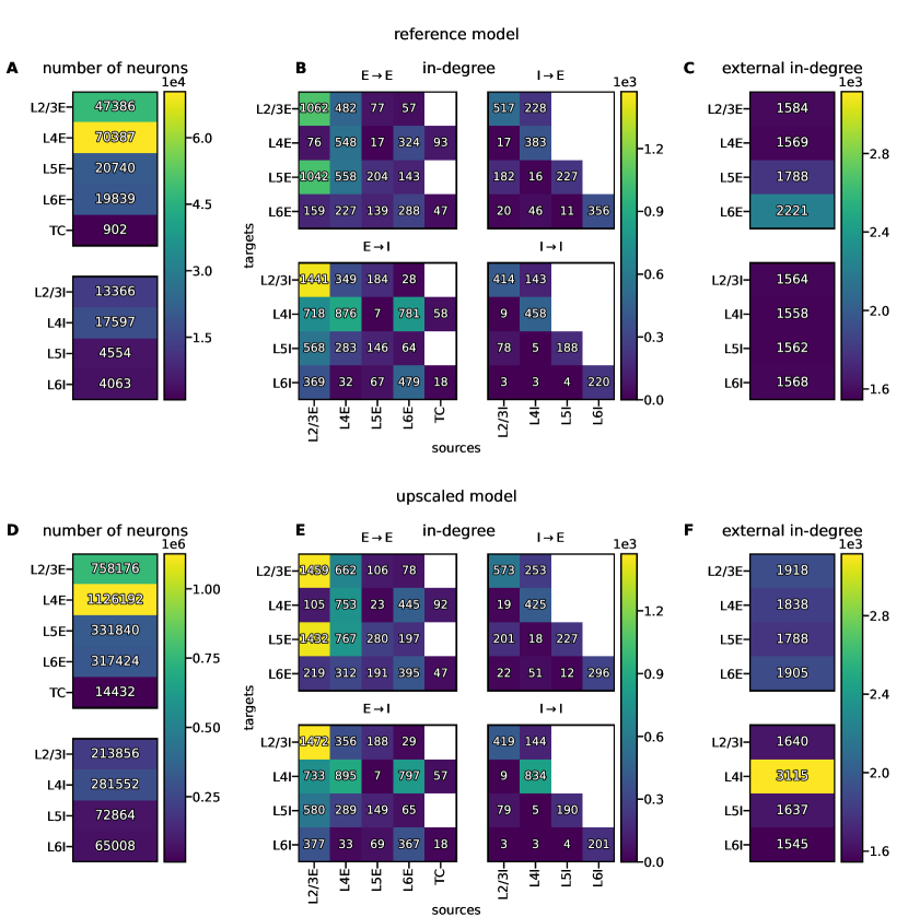
Figure 2: Neuron numbers, average in-degrees of recurrent projections, and external in-degrees. A–C Reference model. D–F Upscaled model. Color codes are identical for in-degrees but not for neuron numbers; values of zero are colorless.

2.2 Forward modeling of extracellular potentials

In the present study we use a well established scheme to compute extracellular potentials from neuronal activity. The method relies on multicompartment neuron modeling to compute transmembrane currents (see, for example, De Schutter and Van Geit, 2009) and volume conduction theory (Nunez and Srinivasan, 2006; Einevoll et al., 2013b), which relates current sources and electric potentials in space. Assuming a volume conductor model that is linear (frequency-independent), homogeneous (the same in all locations), isotropic (the same in all directions), and ohmic (currents depend linearly on the electric field $\mathbf{E}$), as represented by the scalar electric conductivity $\sigma_{\mathrm{e}}$, the electric potential in location $\mathbf{r}\equiv(x,y,z)$ of a time-varying point current with magnitude $I(t)$ in location $\mathbf{r^{\prime}}$ is given by

$$\phi(\textbf{r},t)=\frac{I(t)}{4\pi\sigma_{\text{e}}|\textbf{r}-\textbf{r'}|}.$$ (20)

The potential is assumed to be measured relative to an ideal reference at infinite distance from the source. Consider a set of transmembrane currents of $n_{\mathrm{comp}}$ individual cylindrical compartments indexed by $n$ in an $N-$sized population of cells indexed by $j$ with time-varying magnitude $I_{jn}^{\mathrm{m}}(t)$ embedded in a volume conductor representing the surrounding neural tissue. The extracellular electric potential is then calculated as

$$\phi(\textbf{r},t)=\sum_{j=1}^{N}\sum_{n=1}^{n_{\text{comp}}}\frac{I_{jn}^{\mathrm{m}}(t)}{4\pi\sigma_{\text{e}}}\int\frac{1}{|\textbf{r}-\textbf{r}_{jn}|}\,\mathrm{d}\textbf{r}_{jn}.$$ (21)

The integral term reflects the use of the line-source approximation (Holt and Koch, 1999) which amounts to assuming a homogeneous transmembrane current density per unit length and integrating (LABEL:extracellular1-1) along the center axis of each cylindrical compartment. The thick soma compartments (with $n=1$) with magnitude $I_{j}^{\mathrm{m,soma}}(t)$, however, are approximated as spherical current sources, which amounts to combining Equations 20 and 21 as (Lindén et al., 2014)

$$\phi(\textbf{r},t) =\sum_{j=1}^{N}\frac{1}{4\pi\sigma_{\text{e}}}\left(\frac{I_{j}^{\mathrm{m,soma}}(t)}{|\textbf{r}-\textbf{r}_{j}^{\text{soma}}|}+\sum_{n=2}^{n_{\text{comp}}}\int\frac{I_{jn}^{\mathrm{m}}(t)}{|\textbf{r}-\textbf{r}_{jn}|}\,\mathrm{d}\textbf{r}_{jn}\right)$$

$$=\sum_{j=1}^{N}\frac{1}{4\pi\sigma_{\text{e}}}\left(\frac{I_{j}^{\mathrm{m,soma}}(t)}{|\textbf{r}-\textbf{r}_{j}^{\text{soma}}|}+\sum_{n=2}^{n_{\text{comp}}}\frac{I_{jn}^{\mathrm{m}}(t)}{\Delta s_{jn}}\ln\left|\frac{\sqrt{h_{jn}^{2}+r_{\perp jn}^{2}}-h_{jn}}{\sqrt{l_{jn}^{2}+r_{\perp jn}^{2}}-l_{jn}}\right|\right).$$ (22)

Here, the length of compartment $n$ of cell $j$ is denoted by $\Delta s_{jn}$, the perpendicular distance from the electrode point contact to the axis of the line compartment by $r_{\perp jn}$, and the longitudinal distance measured from the start of the compartment by $h_{jn}$. The distance $l_{jn}=\Delta s_{jn}+h_{jn}$ is measured longitudinally from the end of the compartment. As the above denominators can be arbitrarily small and cause singularities in the computed extracellular potential, we set the minimum separation $|\textbf{r}-\textbf{r}_{j}^{\text{soma}}|$ or $r_{\perp jn}$ equal to the radius of the corresponding compartment.

The above equations assume point electrode contacts, while real electrode contacts have finite extents. We employ the disc-electrode approximation (Camuñas Mesa and Quiroga, 2013; Lindén et al., 2014; Ness et al., 2015)

$$\phi_{\text{disc}}(\mathbf{u},t)=\frac{1}{A_{S}}\iint_{S}\phi(\mathbf{u},t)\,\mathrm{d}^{2}r\approx\frac{1}{m}\sum_{h=1}^{m}\phi({\bf u}_{h},t)$$ (23)

to approximate the averaged potential across the uninsulated contact surface (Robinson, 1968; Nelson et al., 2008; Nelson and Pouget, 2010; Ness et al., 2015). We average the potential ((LABEL:extracellular3-1)) in $m=20$ randomized locations $\mathbf{u}_{h}$ on each circular and flat contact surface $S$ with surface area $A_{S}$ and radius $5\,\mathrm{\mu m}$. The surface normal vector on the disc representing each contact is the unit vector along the vertical $z-$axis. All forward-model calculations are performed with the simulation tool LFPy (https://lfpy.readthedocs.io, Lindén et al., 2014; Hagen et al., 2018), which uses the NEURON simulation software (https://neuron.yale.edu, Carnevale and Hines, 2006; Hines et al., 2009) to calculate transmembrane currents.

2.2.1 The hybrid scheme for modeling extracellular signals

Our study calculates extracellular potentials from point-neuron network models using a modified version of the hybrid modeling scheme by Hagen et al. (2016). The scheme combines the forward modeling of extracellular potentials (i.e., LFPs) on the basis of spatially reconstructed neuron morphologies with recurrent network activity simulated using point-neuron networks. Point-neuron models alone cannot generate an extracellular potential, as the sum of all its in- and outgoing currents is zero. The validity of the hybrid scheme was recently revisited by Hagen et al. (2022). We refer to the Methods section of Hagen et al. (2016) for an in-depth technical description of the implementation for randomly connected point-neuron network models. Here, we only summarize the scheme’s main steps and list the changes incorporated for networks with distance-dependent connectivity and periodic boundary conditions. As in Hagen et al. (2016), we assume that cortical network dynamics are well captured by the point-neuron network, and apply the hybrid scheme as follows:

• Spike trains of individual point neurons are mapped to synapse activation times on corresponding postsynaptic multicompartment neurons while overall connection parameters are preserved, that is, the distribution of delays, the mean postsynaptic currents, the mean number of incoming connections onto individual cells (in-degree), and the cell-type and layer specificity of connections is preserved, as in Hagen et al. (2016).

• The multicompartment neurons are mutually unconnected, and synaptic activations result in transmembrane currents that contribute to the total LFP.

• Activity in multicompartment neuron models (and the corresponding LFP) does not interact with other multicompartment neurons or the activity in the point-neuron network model, that is, there are no synaptic or ephaptic interactions.

• Each population $Y\in X_{\mathrm{total}}\backslash\left\{\mathrm{TC}\right\}$ of neurons in the point-neuron network may map to a number of cell types $y$ in the multicompartment representation . An overview of the choice of morphologies representing each cell type ($M_{y}$), segment count per morphology ($n_{\mathrm{comp}}$), occurrence ($F_{y}$), relative occurrence ($F_{yY}$) per population, and final cell count is given in 5. The corresponding morphologies and layer boundaries are shown in 6.

The first version of the hybrid scheme implemented in hybridLFPy (https://INM-6.github.com/hybridLFPy) is developed for random networks such as the layered cortical microcircuit model of Potjans and Diesmann (2014). In contrast to this model that contains no spatial information, the upscaled model (2.1) assigns spatial coordinates to the neurons within each layer but still ignore information about cortical depth, and draw connections between neurons with probabilities depending on lateral distance. Modifications to the hybrid scheme accounting for spatially organized networks include:

• Multicompartment neuron models inherit their lateral locations from their point-neuron counterparts. Population-dependent somatic depths are defined as in Hagen et al. (2016).

• The spiking activity from all neurons in the point-neuron network is recorded and indexed by the corresponding neuron ID.

• Presynaptic neuron IDs are drawn randomly for each multicompartment neuron governed by the same distance-dependent probability as is used when constructing the point-neuron network. The connectivity is thus statistically reproduced. The same distance-dependent delay rule is also implemented in the hybrid scheme, and can be set separately for each pair of populations.

• The extracellular potential is computed at $100$ contact sites arranged on a square regular grid with each contact separated by $400\,\mathrm{\mu m}$, similar to the layout of the Blackrock ‘Utah’ multi-electrode array, and at a depth corresponding to the center of layer $2/3$ ($\mathrm{L}2/3$). The signal predictions account for periodic boundary conditions as described next.

Layer	Population	Pop. size	Cell type	Morphology	Segments	Occurrence	Rel. occurrence	Cell count
	$Y$	$N_{Y}$	$y$	$M_{y}$	$n_{\mathrm{comp}}$	$F_{y}(\%)$	$F_{yY}(\%)$	$N_{y}$
$2/3$	$\mathrm{L}2/3\mathrm{E}$	$758,176$	p23	p23	$689$	$23.9$	$100.0$	$758,176$
	$\mathrm{L2/3I}$	$213,856$	b23	i23	$324$	$2.9$	$42.5$	$90,816$
			nb23	i23	$324$	$3.9$	$57.5$	$123,040$
$4$	$\mathrm{L4E}$	$1,126,192$	p4	p4	$603$	$11.9$	$33.3$	$375,397$
			ss4(L2/3)	ss4	$339$	$11.9$	$33.3$	$375,397$
			ss4(L4)	ss4	$339$	$11.9$	$33.3$	$375,397$
	$\mathrm{L4I}$	$281,552$	b4	i4	$230$	$7.0$	$78.3$	$220,345$
			nb4	i4	$230$	$1.9$	$21.7$	$61,207$
$5$	$\mathrm{L5E}$	$331,840$	p5(L2/3)	p5v1	$423$	$8.2$	$78.7$	$261,120$
			p5(L5/6)	p5v2	$1078$	$2.2$	$21.3$	$70,720$
	$\mathrm{L}5\mathrm{I}$	$72,864$	b5	i5	$283$	$1.0$	$42.9$	$31,227$
			nb5	i5	$283$	$1.3$	$57.1$	$41,637$
$6$	$\mathrm{L}6\mathrm{E}$	$317,424$	p6(L4)	p6	$456$	$7.5$	$75.1$	$238,506$
			p6(L5/6)	p5v1	$447$	$2.5$	$24.9$	$78,918$
	$\mathrm{L}6\mathrm{I}$	$65,008$	b6	i5	$283$	$1.0$	$50.0$	$32,504$
			nb6	i5	$283$	$1.0$	$50.0$	$32,504$

Table 5: Summary of cell-type specific population and morphology pararameters for extracellular signal predictions via the hybrid scheme.

2.2.2 Modifications of the forward model to account for periodic boundary conditions

As the upscaling procedure of the $1\,\mathrm{mm^{2}}$ reference point-neuron network model incorporates periodic boundary conditions, we modify the calculations of extracellular potentials accordingly. The premise for this modification is that transmembrane currents of a neuron positioned near the lateral network layer boundary should contribute to the extracellular potential as sources across the boundary. This is analogous to input from network connections across the boundaries resulting from the distance-dependent connectivity rule. Here, this modification is implemented by accounting for additional “imaginary” transmembrane current sources. (LABEL:extracellular4-1) computes the extracellular potential at location r by iterating over all true current sources, i.e., each neuron located on the $L\times L$ domain with side length $L$. We assume that the sheet is surrounded by eight identical domains such that the potential at location r in the center sheet receives contributions from within an extended area of size $3L\times 3L$. In other words, for each current source we sum up contributions from across both the true and all eight imaginary sheets, taking into account their distances to r on the notionally extended cortical sheet.

2.3 Model signal predictions

As simulation output, we consider the spiking activity of the point-neuron networks (2.1), and corresponding multi-unit activity (MUA), LFP (2.2) and current-source density (CSD) estimates. We use simulated output data only after an initial period $T_{\mathrm{pre}}$ of model presimulation time to avoid startup transients, and compute all measures for the whole time interval of the subsequent simulation (model times $T_{\mathrm{model,1}}$, $T_{\mathrm{model,2}}$, and $T_{\mathrm{model,3}}$).

2.3.1 Temporal binning of spike trains

Spike times $t_{i}^{\mathrm{s}}$ of the point-neuron networks simulated using temporal resolution $h$ are assigned to bins with width $\Delta t$. Temporally binned spike trains are used to compute pairwise spike-train correlations and population-rate power spectral densities, and to illustrate population-averaged rate histograms. The bin width $\Delta t$ is an integer multiple of the simulation resolution $h$. The simulation duration $T_{\mathrm{model}}$ is an integer multiple of the bin width such that the number of bins is $K=T/\Delta t$. Time bins have indices $k\in\{0,1,...,K-1\}$, spanning time points in $t\in[k\Delta t,(k+1)\Delta t)$.

2.3.2 Spatiotemporal binning of spike trains

In order to compute the propagation speed of evoked activity in the network, we perform a spatiotemporal binning operation of spiking activity in the network. As introduced in 2.1, neuron positions $\left(x_{i},y_{i}\right)$ of the point-neuron network are randomly drawn with $\left\{x_{i},y_{i}\right\}\in$$\left[-L/2,L/2\right)$ . We subdivide the spatial domain of each layer into square bins of side length $\Delta l$ such that the integer numbers of bins along the $x-$ and $y-$axis are $L_{\left\{x,y\right\}}=L/\Delta l$. The bin indices are $l_{\left\{x,y\right\}}\in\{0,1,...,L_{\left\{x,y\right\}}-1\}$, spanning $\left\{x,y\right\}\in[l_{\left\{x,y\right\}}\Delta l-L/2,(l_{\left\{x,y\right\}}+1)\Delta l-L/2)$. Temporal bins of width $\Delta t$ are defined as above. We compute for each population a spatially and temporally binned instantaneous spike-count rate in units of $\mathrm{s^{-1}}$ as the number of spike events from all neurons inside the spatial bin divided by $\Delta t$.

2.3.3 Calculation of the local field potentials (LFP)

The local field potential (LFP) is here defined as the temporally downsampled extracellular signal predicted using the hybrid scheme described in 2.2.1, at a resolution of $\Delta t$. Our workflow uses the decimate function of the scipy.signal package for downsampling by a factor $\Delta t/h$.

2.3.4 Calculation of the current-source density (CSD)

The scheme calculates the current-source density (CSD) from the sum of transmembrane currents within a cuboid around the contact point of each electrode, divided by the corresponding volume (with unit current per volume). This signal is linearly related to the extracellular potential, but without confounding effects by the conductive medium. Each CSD domain $\Omega_{k}$ is defined as having side lengths $400\,\mathrm{\mu m}$ in the lateral $x$- and $y$-dimensions (same as the electrode separation), and thickness $100\,\mathrm{\mu m}$ along the $z$-axis, centered around each electrode location. Then, the CSD of each cuboid indexed by $k$ in each population results from compartmental currents as

$$C_{\Omega_{k}}=\frac{1}{V_{\Omega_{k}}}\sum_{j=1}^{M}\sum_{n=1}^{n_{\text{comp}}}\begin{cases}I_{jn}&\mathrm{\mathrm{if}}\;I_{jn}\;\text{fully inside }\Omega_{k}\\ I_{jn}\frac{\Delta s_{jn,\text{inside}}}{\text{$\Delta s_{jn}$}}&\mathrm{\mathrm{if}}\;I_{jn}\;\text{partially inside }\Omega_{k}\\ 0&\text{otherwise.}\end{cases}$$

Here, $V_{\Omega_{k}}$ denotes the cuboid volume, $\Delta s_{jn}$ compartment length as above, and $\Delta s_{jn,\text{inside}}$ the length of the portion of the compartment inside $\Omega_{k}$. For the the numerical evaluation we use the class VolumetricCurrentSourceDensity provided by the lfpykit Python package (lfpykit.readthedocs.io).

2.3.5 Calculation of the MUA signal

For each electrode located in $\mathrm{L2/3}$, we compute a signal representative of the so-called multi-unit activity (MUA) that is obtained from recordings of extracellular potentials by high-pass filtering the signal ($\gtrsim 500\mathrm{Hz}$), followed by signal rectification, temporal smoothing, and downsampling (see, for example, Einevoll et al., 2007). A biophysical modeling study (Pettersen et al., 2008) shows that this signal is approximately linearly related to the firing rate of the local population of neurons in the vicinity of the measurement device. Neuron coordinates $\left(x_{i},y_{i}\right)$ of the upscaled point-neuron network are randomly drawn on the interval $\left\{x_{i},y_{i}\right\}\in$$\left[-L/2,L/2\right)$. We subdivide the layers into square bins of side length $\Delta l_{\mathrm{MUA}}=0.4\,\mathrm{mm}$ resulting in $10$ bins along the $x-$ and $y-$axis, respectively. The contact point of each electrode is located at the center of the respective bin. In the same way we define temporal bins of width $\Delta t$ and compute for each population a spatially and temporally binned spike-count rate in units of $\mathrm{s^{-1}}$ by tallying the spike events of all neurons inside the spatial bin and dividing by the width of the temporal bin $\Delta t$. We define the MUA signal as the number of spikes per spatiotemporal bin emitted by populations $\mathrm{L2/3E}$ and $\mathrm{L2/3I}$.

2.4 Statistical analysis

2.4.1 Spike rasters and rate histograms

The spike raster diagrams or dot displays show information on spiking activity. Each dot marks a spike event, and the dot position along the horizontal axis denotes the time of the event. Spike data of different neuron populations are stacked and the number of neurons shown is proportional to the population size. As indicated in the respective figure caption, neurons within each population are either scrambled on the vertical axis of the dot display or sorted according to their lateral $x-$position.

We compute population-averaged rate histograms by deriving the per-neuron spike rates in time bins $\Delta t$ and units of $\mathrm{s^{-1}}$, averaged over all neurons per population within the center disc of $1\,\mathrm{mm^{2}}$. The corresponding histogram shows the rates in a time interval of $\pm 25\,\mathrm{ms}$ around the occurrence of a thalamic pulse. Such a display is comparable to the Peri-Stimulus Time Histogram (PSTH, Perkel et al., 1967) that typically shows the spike count summed over different neurons or trials versus binned time.

Image plots with color bars can have a linear or a logarithmic scaling as specified in the respective captions. Since values of the distance-dependent cross-correlation functions can be positive or negative, we plot these with linear scaling up to a threshold, beyond which the scaling is logarithmic.

2.4.2 Statistical measures

Per-neuron spike rates $FR$ are defined as the number of spikes per neuron during each simulation divided by the model time $T_{\mathrm{model}}$. Distributions of per-neuron spike rates are computed from all spike trains of each population separately for an interval from $0$ to $10\,\mathrm{s^{-1}}$ using $30$ bins. Histograms are normalized such that the cumulative sum over the histogram equals unity. We define the mean rate per population $\overline{FR}$ as the arithmetic mean of all per-neuron spike rates of each population.

The coefficient of local variation $LV$ is a measure of spike-train irregularity computed from a sequence of length $n$ of consecutive inter-spike intervals $T_{i}$ (Shinomoto et al., 2003, Equation 2.2), defined as

$$LV=\frac{1}{n-1}\sum_{i=1}^{n-1}\frac{3\left(T_{i}-T_{i+1}\right)^{2}}{T_{i}+T_{i+1}}.$$ (24)

Like the conventional coefficient of variation $CV$ (Shinomoto et al., 2003, Equation 2.1), a sequence of intervals generated by a stationary Poisson process results in a value of unity, but the $LV$ statistic is less affected by rate fluctuations compared to the $CV$; thus, a non-stationary Poisson process should result in $LV\approx 1$. We compute the $LV$ from the inter-spike intervals of the spike trains of all neurons within each population. Distributions of $LV$s are computed from $0$ to $2$ using $30$ bins, and histograms are normalized such that the cumulative sum over the histogram equals unity. We define the mean $LV$ per population $\overline{LV}$ as the arithmetic mean of all $LV$s of each population.

The Pearson (product-moment) correlation coefficient $CC$ is a measure of synchrony that is defined for signals $u\left(t\right)$ and $v\left(t\right)$ as

$$C_{uv}=\frac{C_{uv}\left(0\right)}{\sqrt{C_{uu}\left(0\right)C_{vv}\left(0\right)}},$$ (25)

where

$$C_{uv}(\tau)=\left\langle\left(u\left(t\right)-\left\langle u\left(t\right)\right\rangle_{t}\right)\left(v\left(t+\tau\right)-\left\langle v\left(t\right)\right\rangle_{t}\right)\right\rangle_{t}$$ (26)

denotes the covariance for a time lag $\tau$ (Perkel et al., 1967). For the numerical evaluation of correlation coefficients we use numpy.corrcoef.

To compute distributions of spike-count correlations, $u(t)$ refers to the number $n_{i}(t,\,t+\Delta t_{CC})$ of spikes of neuron $i$ in population $X$ and $v(t)$ to the number $n_{j}(t,\,t+\Delta t_{CC})$ of spikes of neuron $j$ in population $X$ in a time interval $[t,\,t+\Delta t_{CC})$. The bin size $\Delta t_{CC}=2\,\mathrm{ms}$ corresponds to the refractory time. We randomly select $200$ neurons per population and obtain the $CC$ from all disjoint neuron pairs $ij$. Within each population, meaning $X=Y$, the $CC$ is denoted by $E$–$E$ for an excitatory population or $I$–$I$ for an inhibitory population. Correlations between neurons from the excitatory and the inhibitory population in each layer are denoted by $E$–$I$. $CC$ histograms are computed from $-0.02$ to $0.02$ using $30$ bins, and normalized such that the integral over the histogram equals unity.

We also compute distance-dependent spike-count correlations for spike counts from $40$ excitatory and $10$ inhibitory spike trains sampled from L2/3 and plot them according to distance between neuron pairs. To assess distance-dependent correlations between LFP, CSD, and MUA signals, $u$ and $v$ denote the time series recorded at the respective electrode. Here, we fit exponential functions of the form

$$y(r)=a\cdot\mathrm{e}^{-r/b}+c,$$ (27)

where the $n$-tuple $\beta=(a,b,c)$ of constant parameters minimizes the sum $\sum_{i=1}^{m}\left|y_{i}(r_{i})-y(r_{i},\beta))\right|^{2}$ for the $m$ data points $y_{i}$ computed for distance $r_{i}$. The parameter fitting is implemented using a non-linear least squares method (Vugrin et al. (2007), using the implementation curve_fit of the scipy.optimize module), with initial guess $\beta=(0.1,0.1,0.1)$. Goodness of fit is quantified by the coefficient of determination, defined as

$$\mathrm{R}^{2}=1-\frac{\sum_{i=1}^{m}\left(y_{i}(r_{i})-y(r_{i},\beta)\right){}^{2}}{\sum_{i=1}^{m}\left(y_{i}(r_{i})-\overline{y}\right){}^{2}},$$ (28)

where $\overline{y}$ is the mean of the observed data.

Coherences are computed as

$$\gamma_{uv}^{2}(f)=\frac{|\mathcal{S}_{uv}(f)|^{2}}{\mathcal{S}_{uu}(f)\mathcal{S}_{vv}(f)},$$ (29)

where $\mathcal{S}_{uv}(f)$ is the cross-spectral density between $u$ and $v$, and $\mathcal{S}_{uu}(f)$ and $\mathcal{S}_{vv}(f)$ are the power spectral densities (PSDs) of each signal. The cross-spectral density and power spectra are computed using Welch’s average periodogram method (Welch, 1967) as implemented by matplotlib.mlab’s csd and psd functions, respectively, with segment length $N_{\mathrm{FFT}}=256$ (the number of data points per block for the fast Fourier transform), overlap between segments $N_{\mathrm{overlap}}=192$ and signal sampling frequency $F_{\mathrm{s}}=2\,\mathrm{kHz}$. To compute the population-rate power spectral density, we use the spike trains of all neurons per population, resampled into bins of size $\Delta t$, and with the arithmetic mean across time of this population-level signal subtracted.

The effect of thalamic pulses is analyzed by means of distance-dependent cross-correlation functions $CC^{\nu}\left(\tau,r\right)$ evaluated for time lags $\tau$. We discretize the network of size $L\times L$ into an even number of square bins of side length $\Delta l$. The spike trains from all neurons within each spatial bin are resampled into time bins of size $\Delta t$ and averaged across neurons to obtain spatially and temporally resolved per-neuron spike rates. We select spatial bins on the diagonals of the network such that each distance to the center with coordinates $\left(0,0\right)$ is represented by four bins. For $14$ distances from consecutive spatial bins along the diagonal, we compute the temporal correlation function between the rates in the respective spatial bins with a binary vector containing ones at spike times of the thalamic pulses and zeros elsewhere, and then average over the four spatial bins at equal distance. The sequences are normalized by subtracting their mean and dividing by their standard deviation. Correlations between the sequences $u$ and $v$ with time steps $k$ and the length of the sequences $K$ are then computed as

$$CC_{uv}\left(\tau\right)=\frac{1}{K}\sum_{k=1}^{K}u_{k+\tau}v_{k}$$ (30)

for $\tau\in\left[-25,25\right]\,\mathrm{ms}$ in steps of $\Delta t$ using np.correlate. Finally, we subtract the baseline correlation value, obtained by averaging over all negative time lags (before thalamic activation at $\tau=0$), and get $CC^{\nu}\left(\tau,r\right)$.

To estimate the propagation speed $v_{\mathrm{prop}}$ from the cross-correlation functions, we find for each distance the time lag corresponding to the largest $CC^{\nu}$. Values of $CC^{\nu}$ smaller than $5\,\mathrm{\%}$ of the maximum of all $CC^{\nu}$ per population across distances and time lags are excluded. We further exclude distances smaller than the thalamic radius $R_{\mathrm{TC}}^{\mathrm{pulse}}$ plus the spatial width of thalamic projections $\sigma_{\mathrm{TC}}$ because a large part of neurons within this radius are simultaneously receiving spikes directly from thalamus upon thalamic pulses. A linear fit for the distance as function of time lag, $r_{p}\left(\tau\right)=r_{p,0}+v_{\mathrm{prop}}\cdot\tau$, yields the speed $v_{\mathrm{prop}}$.

2.5 Software accessibility

We here summarize the details of software and hardware used to generate the results presented throughout this study. Point-neuron network simulations are implemented using NEST v3.4.0 (Sinha et al., 2023), and Python v3.10.4. We use the same executable model description for the reference and upscaled models and switch between them by adjusting parameters. LFP signals are computed using NEURON v8.2.2 (branch ‘master’ at SHA:93d41fafd), LFPykit v0.5 (https://github.com/LFPy/LFPykit.git, branch ‘master’ at SHA:e5156c0) and LFPy v2.3.1.dev0
(http://github.com/LFPy/LFPy.git, branch ‘master’ at SHA:5d241d6), hybridLFPy v0.2 (https://github.com/INM-6/hybridLFPy, branch ‘master’ at SHA:479c2c4). For parameter evaluation we use the Python package parameters v0.2.1. Analysis and plotting rely on Python with numpy v1.22.3, SciPy v1.8.1, and matplotlib v3.5.2. All simulations and analyses are conducted on the JURECA-DC cluster (Thörnig, 2021). Simulations are run distributed using $16$ compute nodes for both the network and the LFP simulations. The source code to reproduce this study is publicly available on GitHub: https://github.com/INM-6/mesocircuit-model.

3 Results

3.1 Spiking activity of the point-neuron networks

After the description and parameterization of the reference and the upscaled models in 2.1, we here investigate their spiking activity obtained by direct simulation. In 3.1.1 we compare the spontaneous spiking activity of both models, and in 3.1.2 we investigate the response evoked by a transient thalamocortical activation in the upscaled model. Our main objective is to confirm that the upscaling procedure preserves the overall statistics of the reference model, and that the inclusion of space facilitates activity propagating across lateral space.

3.1.1 Spontaneous activity

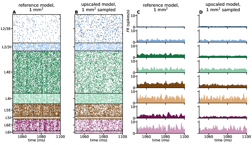
Figure 3: Spike raster plots and instantaneous firing rates. Spike times are vertically organized according to populations defined by layer and neuron type. A Spikes of all neurons of the $1\,\mathrm{mm{{}^{2}}}$ reference model. B Spikes of all neurons located within a center disc of $1\,\mathrm{mm{{}^{2}}}$ in the upscaled model. Neuron IDs within each population are randomized; spatial information is scrambled. C Population-averaged rate histogram with temporal bin size $\Delta t=0.5\,\mathrm{ms}$ of spike data in panel A. D Population-averaged rate histogram with temporal bin size $\Delta t$ of spike data in panel B.

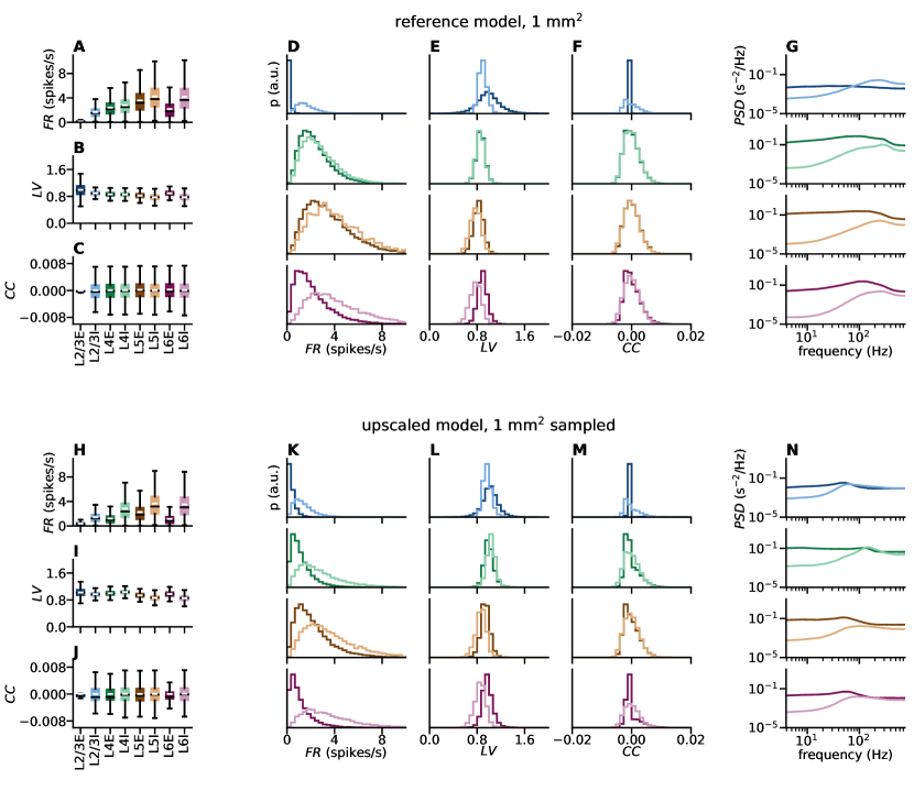
Figure 4: Statistical analysis of the spike data shown in 3. Data of full simulation duration $T_{\text{$\mathrm{model,1}$}}$ analyzed for reference model (top, panels A–G, $1\,\mathrm{mm{{}^{2}}}$) and upscaled model (bottom, panels H–N, $1\,\mathrm{mm{{}^{2}}}$ sampled). A,H Box plots (Tukey, 1977) of spike rates $FR$ for each population (horizontal black lines: median, white lines: mean, boxes in population-specific colors: lower and upper quartiles of the data, whiskers extend to most extreme observations within $1.5\times\text{$\mathrm{IQR}$}$ beyond the $\mathrm{IQR}$ (interquartile range) without outliers (created with matplotlib.pyplot.boxplot). B,I Coefficients of local variation $LV$, see (LABEL:lv). C,J Pearson correlation coefficients $CC$, see (LABEL:CC). D,K Distributions of spike rates $FR$. E,L Distributions of coefficients of local variation $LV$. F,M Distributions of Pearson correlation coefficients $CC$. G,N Population-rate power spectral densities $PSD$.

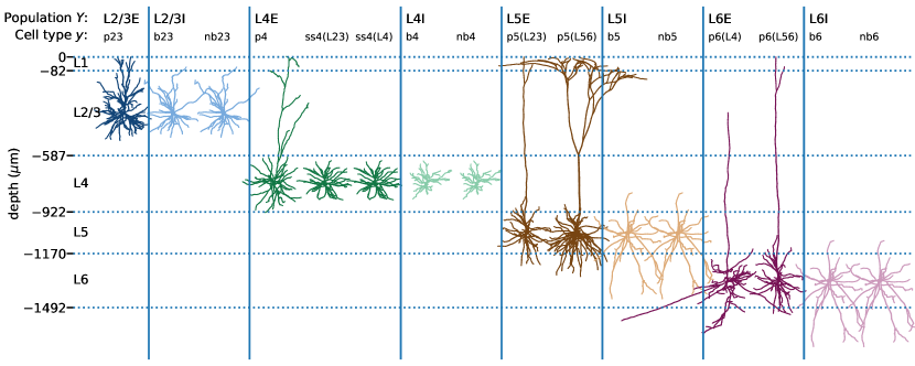
Figure 6: Cell types and morphologies of the multicompartment-neuron populations. The $8$ cortical populations $Y$ in the $4\times 4\,\mathrm{mm^{2}}$ network model are represented by $16$ subpopulations of cell type $y$ with detailed morphologies (Binzegger et al., 2004; Izhikevich and Edelman, 2008). Neuron reconstructions are obtained from cat visual cortex and cat somatosensory cortex (source: NeuroMorpho.org by Kisvárday and Eysel (1992); Mainen and Sejnowski (1996); Contreras et al. (1997); Ascoli et al. (2007); Stepanyants et al. (2007), see Hagen et al., 2016, Table 7). Each morphology is here shown in relation to the layer boundaries across depth (horizontal lines). Colors distinguish between network populations as in 1.

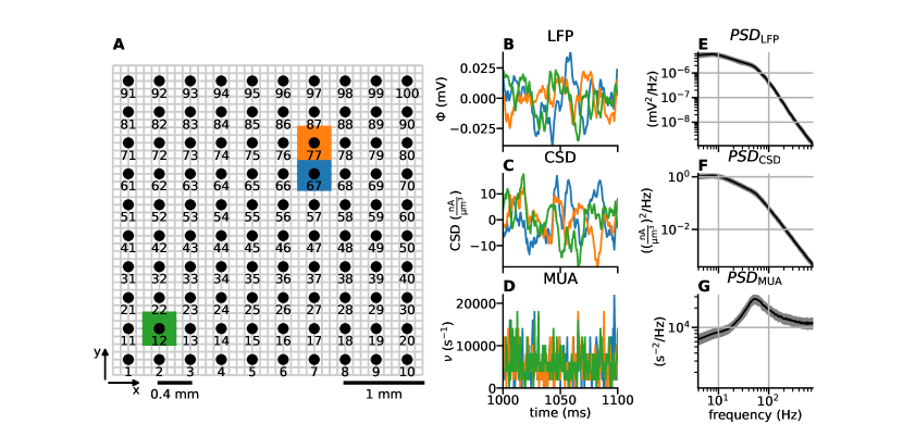
Figure 7: Top-down illustration of multi-electrode array geometry and LFP, CSD, and MUA signals. A Extracellular potentials are computed in $10\times 10$ electrode locations denoted by circular markers at the depth corresponding to the center of layer $\mathrm{2/3}$. The electrode inter-contact distance is $400\,\mathrm{\mu m}$. The signals are computed at the center of layer $\mathrm{2/3}$ (at $z=-334\,\mathrm{\mu m}$) The number under each circular marker denotes the channel number. B–D LFP, CSD, and MUA signal excerpts from three chosen contacts numbered $12$, $67$, and $77$, color code as in panel A. The CSD is computed from transmembrane currents, and the MUA is calculated as the count of excitatory and inhibitory spike events from layer $\mathrm{2/3}$ neurons in spatiotemporal bins of duration $\Delta t=0.5\,\mathrm{ms}$ and width $400\,\mathrm{\mu m}$ around each contact. E LFP power spectrum averaged over channels (black line). The gray area denotes the average spectrum plus/minus one standard deviation computed over all observations. F,G Same as panel E, but for the CSD and MUA signals.

The spike raster plot in 3A and the population-averaged rate histograms in 3C show that the reference model produces asynchronous irregular spiking with firing rates below $10\,\mathrm{spikes/s}$ (Softky and Koch, 1993; Brunel and Hakim, 1999; Brunel, 2000) and rate fluctuations comparable in amplitude to the mean rate for each population. The firing rates are on average higher for inhibitory populations than for excitatory populations within the same layer, and the mean firing rate is larger than the median for each population (see 4A). The latter corresponds to the long-tailed distributions of spike rates in 4D with most neurons firing at lower rates. This type of asymmetric distribution of firing rates in the model resembles the lognormally distributed firing rates observed experimentally (reviewed by Buzsáki and Mizuseki, 2014). The mean values of the coefficients of local variation (4B,E) are close to unity, indicating that the regularity of the spike trains is similar to that of a Poisson point process ($LV=1$). The distributions are broad, that is, a fraction of neurons in each population has spike-train statistics with $LV>1$. The mean $LV$ values are comparable to values observed in visual cortex across different species (Mochizuki et al., 2016, Figure 5B). The box plots in 4A,B are similar to (Potjans and Diesmann, 2014, Figure 6) showing firing rates and the conventional coefficient of variation (Shinomoto et al., 2003, Equation 2.1). The Pearson correlation coefficients ($CC$, 4C,F) are distributed around zero. With our model time of $T_{\mathrm{model,1}}=5\,\mathrm{min}$, the shapes of the distributions observed here are not strongly affected by the finite simulation duration, but they are not fully converged yet. The effects of simulation duration were investigated by Dasbach et al. (2021) using the microcircuit model by Potjans and Diesmann (2014) (see Figures 2 and 7 of Dasbach et al., 2021). Weak pairwise spike-train correlations (with mean values $<0.1$ using $50\,\mathrm{ms}$ count windows) are reported, for example, by Ecker et al. (2010) who record from nearby neurons in primary visual cortex of awake monkey under different stimulation conditions. The population-rate power spectral densities in 4G show that the power tends to be higher in the activity of excitatory compared to inhibitory populations in each layer due to the overall larger density of excitatory neurons, except for layer $2/3$, where the excitatory rate is less than $1\,\mathrm{\text{spike/s}}$. Across layers, the power is highest in layer $4$, explained by the comparatively high spike rates and high cell densities. The power spectra are relatively flat without visible dominant oscillation frequencies.

Analyzing the spike data of all neurons of the upscaled model that are located within the central disc of $1\,\mathrm{mm^{2}}$ yields qualitatively similar spiking statistics to the reference model, as seen by comparing 3 panels A,C versus panels B,D and 4 panels A–G versus H–N. The difference between inhibitory and excitatory firing rates in each layer is more pronounced in the upscaled model. The upscaled model also exhibits a higher excitatory firing rate in layer $2/3$ compared to the reference model.

The scaling factors for recurrent and external in-degrees ($k_{YX}$ and $k_{\mathrm{ext},Y}$ in 4) are chosen based on a dynamic argument: There is accumulating evidence that the typical operating regime of sensory cortices is asynchronous and irregular in particular in the awake state when no specific stimulus is present. Measures of LFP signals, which are assumed to mainly reflect synaptic activity, in for example visual cortex also do not show pronounced peaks in their spectra in the absence of stimuli (see, for example, Berens et al., 2008; Jia et al., 2011; Ray and Maunsell, 2011; Jia et al., 2013a; van Kerkoerle et al., 2014). The reference model already shows reduced global synchrony in the low- and high-gamma ranges compared to the model by Potjans and Diesmann, 2014. We apply the mentioned perturbations to the in-degrees in order to achieve asynchronous-irregular activity at plausible firing rates also in the final upscaled model. Our approach is informed by the analytical framework by Bos et al. (2016) who provide a sensitivity measure that relates population rate spectra to the connectivity of the underlying neuron network. Since the in-degrees in the reference model are estimated across different areas and species and are merely suggestive of typical cortical connectivity, we consider a few modifications to these values to be within the bounds of uncertainties.

In the power spectra of the upscaled model (4H), we observe a mildly pronounced peak at $\sim 50\,\mathrm{Hz}$ across all populations except within layer $4$ where such oscillations are attenuated via the increased in-degree from $\mathrm{L4I}$ onto itself, leaving only a shoulder above $\sim 100\,\mathrm{Hz}$. The low-gamma peak seen around $50\,\mathrm{Hz}$ is predominantly generated by a sub-circuit of layer $2/3$ and layer $4$ populations of excitatory and inhibitory neurons (pyramidal-interneuron gamma or PING mechanism (Leung, 1982; Börgers and Kopell, 2003, 2005; Bos et al., 2016). A high-gamma peak $\gtrsim 200\,\mathrm{Hz}$ resulting from interneuron-interneuron interactions (interneuron-interneuron gamma or ING mechanism, see Whittington et al., 1995; Wang and Buzsáki, 1996; Chow et al., 1998; Whittington et al., 2000) is pronounced in the version of the microcircuit model by Potjans and Diesmann (2014) studied by Bos et al. (2016) but not in the reference model. See Buzsáki and Wang (2012) for a review on the various mechanisms underlying gamma oscillations.

3.1.2 Sensitivity to perturbed parameters during evoked activity

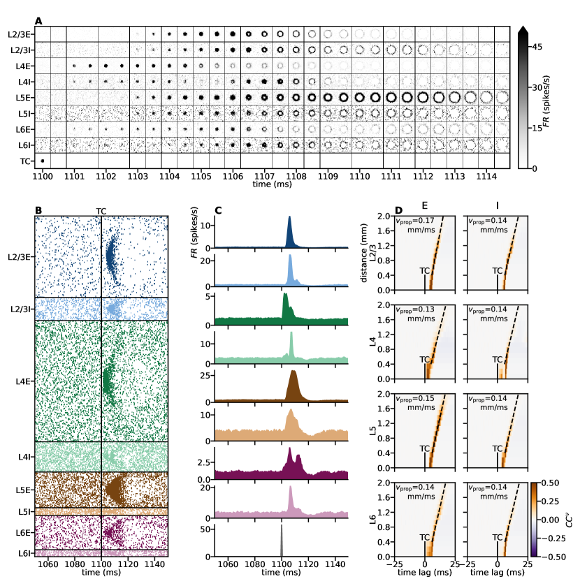
Figure 5: Activity evoked by thalamic pulses. A Series of snapshots of spatiotemporally binned activity per population over the whole $4\times 4\,\mathrm{mm^{2}}$ network. B Spike raster showing every $25$th neuron of all neurons in $4\times 4\,\mathrm{mm^{2}}$; neurons are sorted according to their x-position. The network is stimulated by a single thalamic pulse at $t=1,100\,\mathrm{ms}$. C Population-averaged rate histograms with temporal bin size $\Delta t=0.5\,\mathrm{ms}$ for a time interval around the thalamic pulse. D Distance-dependent cross-correlation functions $CC^{\nu}\left(\tau,r\right)$ between thalamic activation (length of vertical bar indicates radius of patch of active thalamic neurons) and spatially binned spiking activity, where $r$ is the distance to the center of the network and $\tau$ is the time lag. Estimate for wave propagation speed $v_{\mathrm{prop}}$ through linear fit (dashed line).

We have so far only considered networks receiving external inputs with stationary rates. However, cortical areas are recurrently connected to other parts of cortex and subcortical structures, and receive inputs with large rate fluctuations. In order to assess the speed of wave propagation across cortical space, we here mimic a stimulation experiment, by activating all thalamic neurons inside a disc of radius $R_{\mathrm{TC}}^{\mathrm{pulse}}$ centered around $\left(x,y\right)=\left(0,0\right)$ once every time interval of $\Delta t_{\mathrm{TC}}$ (see 4 for values). The activation could for example represent a visual stimulation experiment where activity in lateral geniculate nucleus (LGN, or visual thalamus) thalamocortical ($\mathrm{TC}$) projection neurons is evoked by a brief flash stimulus to a part of the visual field (Bringuier et al., 1999; Muller et al., 2014), air puffs or mechanical whisker deflections to stimulate whisker barrel cortex (Swadlow et al., 2002; Einevoll et al., 2007), or direct electric or optogenetic stimulation of the thalamocortical pathway (Klein et al., 2016). The model of Potjans and Diesmann (2014, page 802) exhibits a handshake principle in response to thalamic pulses due to mutual interactions of excitatory and inhibitory populations, in which the receiving layer inhibits the sending layer as if to signal that it has received the message, so that the sending layer can stop transmitting. We test whether this mechanism is preserved in the upscaled model. Furthermore, we derive the propagation speed of evoked spiking activity spreading outward from the center of stimulation.

5A shows series of snapshots of spatiotemporally binned activity of each population in the full network of size $4\times 4\,\mathrm{mm^{2}}$ (similar to Mehring et al., 2003; Yger et al., 2011, Figure 2). The thalamic pulse is visible at $t=1,100\,\mathrm{ms}$ in the center of the network. The cortical populations respond with a ring-like outward spread of activity that can be described as a traveling wave, in contrast to a stationary bump of activity (Muller et al., 2018). The spike raster in 5B sorts the neurons within each population vertically according to their $x$-position: the activity before the pulse appears to be asynchronous and irregular, and the spatially confined outward spread of high activity caused by the pulse is followed by reduced activity for tens of milliseconds across different populations until the asynchronous-irregular activity is reattained. In Hao et al. (2016, Figure 3) a similar suppression period of tens of milliseconds is observed after a single-pulse electrical micro-stimulation in monkey motor cortex, often followed by a rebound of excitation. The population-averaged rate histograms in 5 highlight the transient network responses. The strong initial response visible in populations $\mathrm{L4E}$ and $\mathrm{L6E}$ is expected since the thalamocortical input targets layers $4$ and $6$ directly (see 4). This evoked activity affects the other network populations via recurrent connections across and within layers. The duration of the activation is overall similar to evoked multi-unit activity (MUA) following whisker stimulation as reported by Einevoll et al. (2007). The multiple peaks in the rate histograms in panel C, most prominent in populations $\mathrm{L4E}$ and $\mathrm{L6E}$, are due to recurrent excitation and inhibition within and across layers. These results are comparable with Potjans and Diesmann (2014, Figure 10) and Hagen et al. (2016, Figure 7), and we therefore conclude that the upscaling procedure does not fundamentally affect the response of the network to transient external input apart from introducing spatial structure.

In order to derive the radial propagation speed of evoked activity, we compute the distance-dependent cross-correlation functions (see 2.4.2) shown in 5D. The propagation speed $v_{\mathrm{prop}}$ is computed separately for each population via the shift of the maximum value of $CC^{\nu}\left(\tau,r\right)$ for time lags $\tau$ with increasing distance $r$. It is to date difficult to observe wave-like activity on the spiking level (Takahashi et al., 2015). However, model predictions for spiking propagation speeds can be compared with other measures, keeping in mind potential differences between spiking activity and population measures such as the LFP. Both types of signals can reflect propagation along long-range horizontal connections (Grinvald et al., 1994; Nauhaus et al., 2009; Takahashi et al., 2015; Zanos et al., 2015), which also includes synaptic processing times, but they are also affected by intrinsic dendritic filtering (Lindén et al., 2010). Muller et al. (2018) remark that macroscopic waves traveling across the whole brain typically exhibit propagation speeds of $1-10\,\mathrm{mm/ms}$, similar to axonal conduction speeds of myelinated white matter fibers in cortex, while mesoscopic waves (as considered here) show propagation speeds of $0.1-0.8\,\mathrm{mm/ms}$, similar to axonal conduction speeds of unmyelinated long-range horizontal fibers within the superficial layers of cortex. For example, LFP signals in visual cortex propagate with similar speeds: Nauhaus et al. (2009) study the propagation of spike-triggered LFPs both in spontaneous activity and with visual stimulation and derive speeds (mean $\pm$ standard deviation) of $0.31\pm 0.23\,\mathrm{mm/ms}$ in cat and $0.24\pm 0.2\,\mathrm{mm/ms}$ in monkey (both anesthetized). Nauhaus et al. (2012) reanalyze the data from Nauhaus et al. (2009) and further report a speed of $0.18\,\mathrm{mm/ms}$ in cat and $0.29\,\mathrm{mm/ms}$ in monkey for the impulse response of ongoing activity; for data from awake monkey (Ray and Maunsell, 2011) they compute a speed of $0.13\,\mathrm{mm/ms}$. Zanos et al. (2015) measure a speed of $0.31\pm 0.08\,\mathrm{mm/ms}$ triggered by saccades in monkey visual cortex. Propagation speeds obtained via voltage-sensitive dye imaging in visual cortex are comparable as well: an average speed of $0.28\,\mathrm{mm/ms}$ with a $75\%$ confidence interval of $0.19$ to $0.55\,\mathrm{mm/ms}$ in cat (Benucci et al., 2007), $0.1-0.25\,\mathrm{mm/ms}$ in monkey (Grinvald et al., 1994), and a range of $0.25-1.35\,\mathrm{mm/ms}$ with median $\pm$ standard deviation of $0.57\pm 0.18\,\mathrm{mm/ms}$ in monkey (Muller et al., 2014). Estimates from monkey motor cortex are in the same range (Rubino et al., 2006; Takahashi et al., 2015; Denker et al., 2018). The derived propagation speeds in our model are $v_{\mathrm{prop}}\in\left[0.13,0.17\right]\,\mathrm{mm/ms}$, which is within the range of experimentally measured propagation speeds. Note that these values are smaller than the fixed conduction speed ($v=0.3\,\mathrm{mm/ms}$) because propagation through the network includes neuronal integration and the delay offsets.

3.2 Prediction of extracellular signals

We here summarize our findings for the calculated LFP, CSD and MUA signals across the cortical space spanned by the upscaled network model, with recording geometry similar to a $4\times 4\,\mathrm{mm^{2}}$ Utah multi-electrode array. As in Hagen et al. (2016), the eight cortical network populations spanning layers $2/3$, $4$, $5$ and $6$ are expanded into $16$ different cell types in order to account for differences in laminar profiles (layer specificities) of synaptic connections among cell types in a single layer when predicting the LFP. We here refrain from discussing the detailed derivation of laminar profiles from the anatomical data (i.e., Binzegger et al., 2004) as it is given in Hagen et al., 2016 (see also 2.2.1). In 6 we show the reconstructed morphology used for each cell type $y$ in population $Y$, with occurrences and compartment counts summarized in 5. The cortical layer boundaries and depths are also shown in the figure, and each morphology is positioned such that the soma is at the center of the corresponding layer. Different cell types belonging to the same population within a layer may have different geometries supporting different laminar profiles of synaptic connections. This is the case for example for the p4 pyramidal cell type versus the ss4 spiny stellate cell types that both belong to population $\mathrm{L4E}$ of the point-neuron network. Previous modeling studies demonstrate the major effect of the geometry of the morphology on the measured extracellular potential due to intrinsic dendritic filtering of synaptic input (e.g., Lindén et al., 2010, 2011; Łęski et al., 2013), which is also accounted for here.

The geometry of the recording locations corresponding to the $4\times 4\,\mathrm{mm^{2}}$ Utah multi-electrode array is illustrated in 7A. 7B shows example LFP signal traces corresponding to the spontaneous activity in our laminar, upscaled point-neuron network, with spike raster plot shown in 3B. The LFP signal fluctuates with amplitudes somewhat smaller than experimentally observed spontaneous potentials ($0.1-1\,\mathrm{mV}$, Maier et al., 2010; Hagen et al., 2015; Reyes-Puerta et al., 2016; Rimehaug et al., 2023), with occasional transients above $50\,\mathrm{\mu V}$ (not shown). This result is expected as there are no external sources of rate fluctuations and associated LFPs such as thalamic activation or feedback from other areas, which may otherwise explain larger signal amplitudes. The amplitudes observed here are also smaller than those from the forward-model predictions of LFPs from spontaneous activity in a $1\,\mathrm{mm^{2}}$ network model (Potjans and Diesmann, 2014; Hagen et al., 2016, Figure 8M), although the total number of neurons in the upscaled model is greater by a factor of $\sim 40$. The discrepancy is explained by strong gamma oscillations generated in the $1\,\mathrm{mm^{2}}$ network model (Hagen et al., 2016).

For comparison with the LFP, we show in 7C the corresponding CSD signal computed from transmembrane currents in the same locations. The LFP and corresponding CSD in general reflect correlations in synaptic input nearby the measurement site and therefore contain contributions from both local and remote neuronal activity (Kajikawa and Schroeder, 2011; Lindén et al., 2011; Łęski et al., 2013; Rimehaug et al., 2023). The CSD reflects the gross in– and outgoing transmembrane currents in vicinity to the recording device (Nicholson and Freeman, 1975; Mitzdorf, 1985; Pettersen et al., 2006, 2008; Potworowski et al., 2012), and is therefore expected to be less correlated across space than the LFP, which is affected by volume conduction. By visual inspection (7C), the CSD traces of neighboring locations are more similar to each other than to the trace of a more distant location. In contrast, the similarity of the corresponding LFPs (7B) does not show a dependence on distance, reflecting the effect of volume conduction.

The high-frequency ($\gtrsim 100\,\mathrm{Hz}$) part of experimentally obtained extracellular potentials contains information on spiking activity of local neurons (see e.g., Einevoll et al., 2012). Spikes of single neurons may be extracted from the raw signal based on classification of extracellular waveforms of the action-potentialss (through spike sorting, Quiroga 2007; Einevoll et al. 2012). Even if no units are clearly discernible in the high-frequency part of the signal, a previous forward-modeling study using biophysically detailed neuron models (Pettersen et al., 2008) shows that the envelope of the rectified high-pass filtered ($750\,\mathrm{Hz}$ cutoff frequency) signal correlates well with the spike rate in the local population of neurons. In their study, the authors refer to this rectified signal as the multi-unit activity (MUA), which we approximate by summing up the spiking activity of layer $2/3$ neurons in $400\times 400\,\mathrm{\mu m^{2}}$ spatial bins around each contact and weighting the contributions from excitatory and inhibitory neurons identically. These MUA signals have more high-frequency content than the LFP and CSD signals at the same locations (7D). To quantify this observation, we next compare the power spectra.

3.2.1 Signal power spectra

As a first quantitative inspection of the different virtual measurements of network activity, we compute the mean PSDs of LFP, CSD, and MUA signals and their standard deviations in all channels (7E-G). The population firing rate spectra exhibit a gamma oscillation around $50\,\mathrm{Hz}$ (4N). The oscillation is prominent in the MUA signals, due to MUA directly reflecting the firing rates. LFP and CSD express the gamma oscillation merely as a shoulder in the respective PSD. Above $\sim 50\,\mathrm{Hz}$, the signal power of the LFP and CSD decay steeply (approximately as $1/f^{2}$), mainly explained by the combination of intrinsic dendritic filtering (Lindén et al., 2010) and synaptic filtering as modeled using exponential temporal kernels for the synaptic currents. This low-pass filtering effect is absent in the population firing rates and in the MUA signal PSD, which flattens out towards higher frequencies. At frequencies $\lesssim 50\,\mathrm{Hz}$, the LFP and CSD increase in power down to $\sim 10\,\mathrm{Hz}$, below which their spectra remain comparatively flat, in contrast to the drop in MUA power towards low frequencies. Monotonically decreasing LFP signal amplitudes with frequency are consistent with experimental observations (see, e.g., Jia et al., 2011; Prakash et al., 2021).

The lack of low-frequency power in the MUA is partly explained by the background input with a flat power spectrum (a Poisson process with fixed rate) and the absence of recurrent sub-circuits capable of generating slow rate fluctuations or slow oscillations. One mechanism contributing to the lack of low-frequency power in the MUA is active decorrelation by inhibitory feedback, which suppresses population-rate fluctuations (Tetzlaff et al., 2012; Helias et al., 2014).

Having established that the upscaled network yields LFP power spectra in qualitative agreement with experimental observations, we investigate the properties of these signals in terms of distance-dependent correlations and coherences.

3.2.2 Distance-dependent correlations of spike trains and LFPs

The observation of weak pairwise spike-train correlations in cortical neuronal networks (for example, Ecker et al., 2010) is seemingly at odds with the typical observation of highly correlated LFPs across cortical space (for example, Nauhaus et al., 2009). We have so far established that the mean pairwise spike-train correlations within populations in our spatially organized layered network are typically near zero for spontaneous activity (3.1.1). However, the network can propagate waves of synchronous activity when excited by external input (3.1.2). Here, we focus on spontaneous activity, as it is unclear how this weakly correlated network activity affects population signals such as the LFP across space. Previous modeling studies highlight the crucial role of correlation in synaptic inputs for the spatial reach of the LFP (Lindén et al., 2011; Łęski et al., 2013). In contrast to these studies, which rely on input spike trains with Poisson inter-spike statistics, we here account for ongoing network interactions (in particular correlations), and the full numbers of neurons and connections under $4\times 4\,\mathrm{mm^{2}}$ of cortical surface.

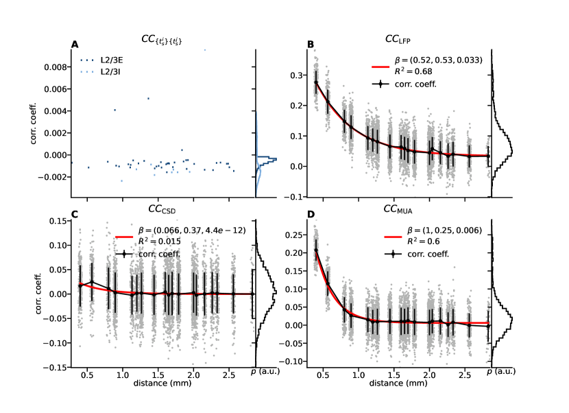
Figure 8: Distance-dependent correlations in spike trains, LFP, CSD, and MUA signals in $\mathrm{L2/3}$. A Pairwise spike-train correlations (vertical) computed for pairs of excitatory (E–E, $n=40$) and inhibitory (I–I, $n=10$) $\mathrm{L2/3}$ neurons (color code in legend), sorted by inter-neuron distance $r$ (horizontal) and gathered across all distances as marginal distributions (vertically, right side of panel). The correlations are computed from spike trains of a network simulation with long model time ($T_{\mathrm{model,1}}=5\,\mathrm{min}$). B Pearson correlation coefficient between pairs of LFP signals as function of separation between channels. The black curve shows the mean at each unique separation (marginal as in panel A); whiskers denote one standard deviation. The red curve shows the least-squares fit of an exponential function ((LABEL:exponential)) to all data points (coefficient of determination ($\mathrm{R}^{2}$) in legend). C Similar to panel B but for CSD signals. D Similar to panel B but for MUA signals. Histograms of the values marginalized across distance are given at the right of each panel. Note that the distance values in panels B–D result from the electrode layout (see 7A); for visibility, the individual data points are jittered along the x-axis by adding uniformly distributed random numbers in $\left[-0.025,0.025\right]$.

For spontaneous spiking activity in the upscaled network, we analyze the LFP, CSD, and MUA across the $100$ channel locations in layer $2/3$ illustrated in 7A, with panels B–D showing temporal snapshots of each signal in three different channels. In addition to pairwise spike train correlations computed for a subset of neurons in network populations $\mathrm{L}2/3\mathrm{E}$ and $\mathrm{L}2/3\mathrm{I}$ arranged by their separation (8A), we compute the Pearson product-moment correlation coefficient between all possible pairs of LFP channels, and sort them by inter-contact distance (8B). Due to the periodic boundary conditions of the upscaled network and LFP model, the largest possible separation between contacts is $L/\sqrt{2}\approx 2.8\,\mathrm{mm}$ (i.e., five electrode contacts along the diagonal). The mean values are well fit by a simple exponential function, with a space constant of $\sim 0.53\,\mathrm{mm}$ and an offset of $\sim 0.03$. The correlations in the simulated LFP (marginal distribution across all distances in 8B) are lower compared to findings by Nauhaus et al. (2009, Fig. 8) during spontaneous activity in anesthetized macaque (approximately $0.95$ at $0.4\,\mathrm{mm}$ and $0.75$ at $2.4\,\mathrm{mm}$ electrode separation, respectively) and cat (approximately $0.93$ at $0.4\,\mathrm{mm}$ and $0.83$ at $2.4\,\mathrm{mm}$ electrode separation, respectively). However, with high-contrast drifting grating type stimuli the correlations between pairs of LFP signals are shown to decrease to values around $0.5$ at an electrode separation of $2.4\,\mathrm{mm}$. Also Destexhe et al. (1999) analyze spatial correlations in the LFP of cat suprasylvian cortex during awake and different sleep states, and find mean correlations of approximately $0.6$ at $2\,\mathrm{mm}$ contact separation in the awake state. The point neuron and corresponding LFP model also ignore rate fluctuations in their background input (here represented as Poisson generators with fixed rates), which may be another source of spatial correlations in vivo. Global fluctuations or shared input correlations in the background input can be expected to increase pairwise LFP correlations (Lindén et al., 2011; Łęski et al., 2013; Hagen et al., 2016).

We next bring our attention to the CSD signal in (8C). By design, the calculated CSD is expected to suppress correlations among channels due to volume conduction and represents the local sink/source pattern underlying the LFP (Nicholson and Freeman, 1975; Mitzdorf, 1985; Pettersen et al., 2006, 2008; Potworowski et al., 2012). The overall positive correlations observed for the LFP are mostly gone for the CSD: the correlations are on average only positive at short separations and negligible beyond $1\,\mathrm{mm}$ electrode separation. This negligible correlation at greater distances reflects in part that dendrites of each morphology (cf. 6) are mostly confined within $\sim 300\,\mathrm{\mu m}$ in the lateral directions. It is important to point out that the CSD estimate (cf. 2.3.4) is here computed at a single depth only, but CSDs do vary across depth, mediated mainly by the apical dendrites of the pyramidal cell populations across layers.

The MUA estimate based on the sum of spiking activity in layer $2/3$ in the vicinity of each LFP contact point (cf. 2.3.5) results in the distance-dependent correlations in 8D. In contrast to pairwise spike-train correlations (8A), a monotonically decaying distance dependence is observed, which is well fit by an exponential function with spatial decay constant of $\sim 0.25\,\mathrm{mm}$ and vanishing offset from zero at greater distances. This sharper decay, about half of the spatial decay constant observed for the LFP, reflects the fact that the LFP is essentially composed of spatiotemporally filtered spiking activity..

3.2.3 Spatial coherence of local field potential is band-passed

So far we have established that the model LFP is correlated across distance in qualitative agreement with experimental findings, while the corresponding CSD and MUA signals are hardly correlated beyond electrode separations of $\sim 1\,\mathrm{mm}$. We next extend this analysis to the frequency domain by considering distance-dependent coherences. This step is mainly motivated by two experimental observations: LFP coherence across channels depends on inter-electrode distance as reported by Jia et al. (2011) and Srinath and Ray (2014), and a study by Dubey and Ray (2016) showing that the ‘spatial spread’ of LFP has band-pass properties in the gamma range. Another modeling study (Łęski et al., 2013) extends the study of LFP ‘reach’ by Lindén et al. (2011) to distance-dependent coherences, showing that dendritic filtering (Lindén et al., 2010) introduces a low-pass effect on the LFP reach of uncorrelated synaptic input currents with an approximately white power spectrum. In contrast to these latter modeling studies, our combined point-neuron network and LFP-generating setup allows accounting for weakly correlated spiking activity in the network, at realistic density of neurons and connections. In contrast to the earlier model studies, the network’s spiking activity is non-random and the corresponding firing rate spectra is frequency dependent (4N), which may allowing testing the hypothesis that network activity in the gamma range results in increased coherence in the LFP, explaining the apparent band-pass filter effect.

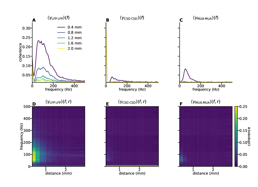
Figure 9: Distance dependence of LFP, CSD, and MUA coherences in $\mathrm{L2/3}$. A Pairwise LFP coherences as function of frequency for different spatial separations (color-coded) between electrode contacts, averaged over pairs with identical distance. B Similar to panel A but computed using the CSD signal at each electrode. C Similar to panels A and B but computed using the MUA signal at each electrode. D–F Coherence (color bar) of LFP, CSD, and MUA respectively as a function of frequency (vertical) and distance between contacts (horizontal).

From the spectrum of the spontaneous LFP (7E) we infer that a fraction of its variance is due to a low-frequency gamma oscillation around $50\,\mathrm{Hz}$ mainly explained by the PING mechanism generated by intra-layer and across-layer interactions between the excitatory and inhibitory network populations (Bos et al., 2016). In 9A we show the mean coherences $\langle\gamma_{\mathrm{LFP-LFP}}\rangle(f)$ between individual pairs of LFP signals from channels separated by a distance $r=\left\{0.4,\,0.8,\,1.2,\,1.6,\,2.0\right\}\,\mathrm{mm}$. The coherence drops quickly from $0\,\mathrm{Hz}$ to around $15\,\mathrm{Hz}$. For the shortest separation ($0.4\,\mathrm{mm}$), the coherence is around $0.05$ at this frequency, and increases above $\sim 0.2$ in the low-gamma range (around $50\,\mathrm{Hz}$). A broad peak in the coherence with magnitudes above 2 is seen up to $100-150\,\mathrm{Hz}$ . Beyond this frequency range, the coherence drops to below $0.1$. The coherence across all frequencies is further reduced for increased inter-contact distances, and is negligible at $2\,\mathrm{mm}$ across all frequencies. The drop in coherence across frequencies with distance is similarly observed in experimental LFP data during stimulus conditions (Srinath and Ray, 2014, Figure 1A). Srinath and Ray (2014) observe a peak in low-gamma LFP coherence around $40\,\mathrm{Hz}$ for distances up to $4\,\mathrm{mm}$ in two different subjects. Also an increase in coherence is seen for harmonic frequencies around $80\,\mathrm{Hz}$. The baseline coherence (no visual stimulus) shows no increase in the gamma range of frequencies, except for sharp peaks due to the CRT display frequency and the second harmonic of noise (Srinath and Ray, 2014). While less pronounced than in their study, also the LFP predictions show elevated coherences across greater distances than the CSD and MUA. The effect is quite visible in the color image plot (9D), compared to the corresponding CSD and MUA (panels E and F). The effect is reminiscent of the apparent band-pass filter effect reported by Dubey and Ray (2016), in that the coherence across sites is increased and decays more slowly with distance in the gamma range compared to higher and lower frequencies. In our study, the effect occurs in the absence of temporally varying external input to the network model. Note that in a previous model iteration (Senk et al., 2018), we reported much stronger LFP coherence in the gamma band across space, attributed to the fact that the network generated relatively strong gamma oscillations, translating into a greater band-pass filter effect.

4 Discussion

This study investigates a multi-layer point-neuron network model covering $4\times 4\,\mathrm{mm^{2}}$ of cortical surface at realistic neuron and connection density, amounting to $\sim 3.2$ million neurons and $\sim 7.7$ billion synapses. The model covers the same area as the $10\times 10$ Utah multi-electrode array and accounts for spiking activity across excitatory and inhibitory neurons in layers $2/3$, $4$, $5$, and $6$, and local field potentials (LFP), current source densities (CSD), and multi-unit activity (MUA) in layer $2/3$. Our model extends a $1\,\mathrm{mm^{2}}$ cortical microcircuit model of macaque V1 (Potjans and Diesmann, 2014; Schmidt et al., 2018a), introducing distance-dependent connection probabilities and delays. The biophysics-based LFP predictions rely on a scheme (Hagen et al., 2016) that is here generalized to spatially structured networks.

The upscaled model reproduces asynchronous-irregular spiking activity, heterogeneous firing rates, spike-train variability consistent with observations in sensory cortex, and weak pairwise spike-train correlations. The model further exhibits spatially spreading activity with plausible propagation speeds evoked by thalamic pulses, comparable to experiments with a brief stimulus to a part of the visual field. Finally, the model accounts for spatially correlated and coherent LFPs during spontaneous network activity. LFP coherences are distance-dependent with a slower spatial decay around the $50\,\mathrm{Hz}$ low-gamma frequency compared to other frequencies, resulting in an apparent band-pass filter effect.

To our knowledge, this study is the first to address both spiking activity and LFP in a layered network model covering several square millimeters of cortical surface at full neuron and synapse density. Compared to natural cortical neuron densities of $\mathcal{O}\left(10^{5}\right)\text{ neurons/mm}^{2}$ (see, e.g., Herculano-Houzel, 2009; Ribeiro et al., 2013), other studies of 2D networks often consider only one layer of excitatory and inhibitory neurons (Mehring et al., 2003; Yger et al., 2011; Voges and Perrinet, 2012; Keane and Gong, 2015; Schnepel et al., 2015) or two layers (Rosenbaum et al., 2017; Antolík et al., 2018), examine a smaller surface area (e.g., only $1\,\mathrm{mm^{2}},$ see Yger et al., 2011; Rosenbaum and Doiron, 2014; Pyle and Rosenbaum, 2017), and use reduced densities (e.g., about $50,000$ neurons on $5\times 5\,\mathrm{mm^{2}}$, Voges and Perrinet, 2012). Tomsett et al. (2014) also incorporate LFP predictions from a network of $\mathcal{O}\left(10^{5}\right)$ multicompartment neurons, but consider only a thin cortical slice across layers similar to in vitro experiments. Network downscaling without compromising first- and second order spike-train statistics requires adjusting connection strengths and background input to the decreased numbers of synapses (van Albada et al., 2015), but upscaling is different: Our procedure of increasing the size of a microcircuit modifies in-degrees and background input, but preserves local recurrence and local activity statistics.

The modeled LFP amplitudes agree with spontaneous LFP amplitudes in the range $0.1-1\,\mathrm{mV}$ observed experimentally (e.g., Maier et al., 2010; Hagen et al., 2015; Reyes-Puerta et al., 2016). The LFP spectra reveal an oscillation around $50\,\mathrm{Hz}$, but otherwise decrease in power with frequency, akin to the power law scaling behavior in experiments. Visual cortex exhibits elevated LFP gamma power in the $30-80\,\mathrm{Hz}$ range especially during stimuli (Jia et al., 2011; Ray and Maunsell, 2011; Berens et al., 2008; Xing et al., 2012; Veit et al., 2017; Katzner et al., 2009; Jia et al., 2013b; Hadjipapas et al., 2015; Ray, 2022), leading to the hypothesis that gamma oscillations have a functional role for computation (Ray and Maunsell, 2010; Jia et al., 2013a; Buzsáki and Wang, 2012). The oscillations here result from the interplay between the excitatory and inhibitory network populations (Bos et al., 2016). The network receives an external drive with a stationary rate, does not intrinsically generate slow rate fluctuations, and is subject to active decorrelation (Tetzlaff et al., 2012). Nevertheless, the model produces correlated LFPs with a distance dependence compatible with experimental observations (Nauhaus et al., 2009). The model also reproduces elevated coherences in the low-gamma band compared to other frequencies, as also seen during visual stimulation (Jia et al., 2011; Srinath and Ray, 2014). The slower spatial decay around $50\,\mathrm{Hz}$ in the model is consistent with a reported increased spatial LFP ‘reach’ analogous to spatial band-pass filtering in the low-gamma band (Dubey and Ray, 2016). Our model shows that this effect is related to network oscillations.

The upscaled model uses exponentially decaying connection probabilities, but future work may incorporate long-range connections. Pyramidal neurons can have long horizontal axons spanning several millimeters in addition to local axonal branching. In cat and monkey visual cortex, these connections are typically patchy and connect neurons with similar orientation selectivity (Livingstone and Hubel, 1984; Gilbert and Wiesel, 1989; Bosking et al., 1997; Tanigawa et al., 2005; Buzás et al., 2006; Binzegger et al., 2007). Some inhibitory interneurons can also exhibit long-range connections (McDonald and Burkhalter, 1993). Voges and Perrinet (2012) demonstrate that the fraction of local versus remote connections is crucial for the resulting network dynamics.

There are only a few comprehensive datasets detailing (distance-dependent) connection probabilities (e.g., Binzegger et al. 2004; Reimann et al. 2017). Most connectivity studies focus on specific projections, and due to different experimental protocols, each with their own limitations (van Albada et al., 2022), the data are difficult to integrate. Neuron morphology appears to provide a valid first approximation for the distance dependence of projections (Amirikian, 2005; Brown and Hestrin, 2009; Hill et al., 2012), but the overlap between dendrites and axons alone does not explain connectivity patterns, due to target neuron-type specificity (Potjans and Diesmann, 2014), specificity at the level of individual neurons (Kasthuri et al., 2015), and preferential locations of dendritic spines and synaptic boutons (Ohana et al., 2012). Algorithmic approaches pursued within large-scale consortia (e.g., Kandel et al., 2013; Markram et al., 2015; Reimann et al., 2015) will hopefully provide more accurate connectomes of different brain regions.

Activity in laminar networks depends on the boundary conditions. Here we use periodic boundary conditions, which is a common choice for 2D models with isotropic connectivity mimicking a patch of the intact brain (e.g., Yger et al., 2011; Voges and Perrinet, 2012; Rosenbaum and Doiron, 2014). However, propagating activity may travel across the boundary and directly influence its own propagation, resulting in wave-front annihilation (Muller et al., 2018). An option to suppress such effects would be to sample the activity of neurons across an inner domain of a larger network (cf. Figures 3 and 4). Larger models could also address the effects of borders to adjacent cortical areas, as anatomical borders between areas affect wave propagation (Xu et al., 2007; Muller et al., 2014).

Spontaneous activity in our models is driven by uncorrelated external inputs with a fixed rate and Poisson statistics that represent connections from remote and neighboring cortices, subcortical structures, and sensory inputs. However, mutual interactions between recurrently connected areas are expected to affect their input statistics in terms of rates, spectra, and correlations (Schuecker et al., 2017; Schmidt et al., 2018a). More detailed models (e.g., Martínez-Cañada et al., 2018) representing naturalistic visual input to cortex are emerging. A recent study relying on a detailed reconstruction of mouse visual cortex showcases the importance of thalamocortical and cortico-cortical input and feedback to the local circuit for evoked LFP and CSD signals (Billeh et al., 2020; Rimehaug et al., 2023).

In terms of signal predictions, the tool LFPy (LFPy.rtdf.io; Hagen et al., 2018) facilitates the calculation of current dipole moments and associated electroencephalographic (EEG) signals and magnetoencephalographic (MEG) signals (Hämäläinen et al., 1993; Nunez and Srinivasan, 2006; Hagen et al., 2018). Forward-model predictions of macroscopic signals like EEG and MEG may thus provide an avenue towards a mechanistic understanding of visually evoked potentials (Sokol, 1976; Neymotin et al., 2020).

Simulations of networks with $\mathcal{O}\left(10^{6}\right)$ neurons can be performed routinely on high-performance computing facilities (Kunkel et al., 2017; Jordan et al., 2018). However, extracellular signal predictions via the hybrid scheme used here, which feeds spikes from the point neuron network to morphologically detailed neurons, are computationally demanding at this scale, requiring $\mathcal{O}(10^{4})$ core hours per simulated second of network activity. Future work can adapt the kernel-based scheme of Hagen et al. (2022) for LFP, EEG, and MEG to spatially organized networks.

The present work represents a stepping stone for interpreting experimental data obtained by multi-electrode arrays on the mesoscale. Simulated single-neuron and population activities can be directly compared with corresponding data in a fully digitized “integrative loop”, while the model’s simplicity makes mathematical analysis in terms of mean-field and neural field theory viable (Bos et al., 2016; Senk et al., 2020). Our hope is that the model facilitates a principled understanding of the dependence of spike correlations on distance, spatially coherent and correlated LFPs, spike-LFP relationships, and emergent spatiotemporal patterns such as waves. We therefore envision the model as a platform for future work adding further constraints iteratively and incrementally to deliver accurate predictions of brain activity.

References

- Abeles (1991) Abeles M (1991) Corticonics: Neural Circuits of the Cerebral Cortex Cambridge University Press, Cambridge, 1st edition.
- Amirikian (2005) Amirikian B (2005) A phenomenological theory of spatially structured local synaptic connectivity. PLOS Comput. Biol. 1:e11.
- Andersen et al. (1978) Andersen P, Silfvenius H, Sundberg SH, Sveen O, Wigström H (1978) Functional characteristics of unmyelinated fibres in the hippocampal cortex. Brain Res. 144:11–18.
- Antolík et al. (2018) Antolík J, Monier C, Frégnac Y, Davison AP (2018) A comprehensive data-driven model of cat primary visual cortex. BioRxiv .
- Ascoli et al. (2007) Ascoli GA, Donohue DE, Halavi M (2007) NeuroMorpho.org: A central resource for neuronal morphologies. J. Neurosci. 27:9247–9251.
- Avermann et al. (2012) Avermann M, Tomm C, Mateo C, Gerstner W, Petersen C (2012) Microcircuits of excitatory and inhibitory neurons in layer 2/3 of mouse barrel cortex. J. Neurophysiol. 107:3116–3134.
- Benucci et al. (2007) Benucci A, Frazor RA, Carandini M (2007) Standing waves and traveling waves distinguish two circuits in visual cortex. Neuron 55:103–117.
- Berens et al. (2008) Berens P, Keliris GA, Ecker AS, Logothetis NK, Tolias AS (2008) Comparing the feature selectivity of the gamma-band of the local field potential and the underlying spiking activity in primate visual cortex. Front. Syst. Neurosci. 2:1–9.
- Berg-Johnsen and Langmoen (1992) Berg-Johnsen J, Langmoen IA (1992) Temperature sensitivity of thin unmyelinated fibers in rat hippocampal cortex. Brain Res. 576:319–321.
- Billeh et al. (2020) Billeh YN, Cai B, Gratiy SL, Dai K, Iyer R, Gouwens NW, Abbasi-Asl R, Jia X, Siegle JH, Olsen SR et al. (2020) Systematic integration of structural and functional data into multi-scale models of mouse primary visual cortex. Neuron 106:388–403.e18.
- Binzegger et al. (2004) Binzegger T, Douglas RJ, Martin KAC (2004) A quantitative map of the circuit of cat primary visual cortex. J. Neurosci. 39:8441–8453.
- Binzegger et al. (2007) Binzegger T, Douglas RJ, Martin KAC (2007) Stereotypical bouton clustering of individual neurons in cat primary visual cortex. J. Neurosci. 27:12242–12254.
- Börgers and Kopell (2003) Börgers C, Kopell N (2003) Synchronization in networks of excitatory and inhibitory neurons with sparse, random connectivity. Neural Comput. 15:509–538.
- Börgers and Kopell (2005) Börgers C, Kopell N (2005) Effects of noisy drive on rhythms in networks of excitatory and inhibitory neurons. Neural Comput. 17:557–608.
- Bos et al. (2016) Bos H, Diesmann M, Helias M (2016) Identifying anatomical origins of coexisting oscillations in the cortical microcircuit. PLOS Comput. Biol. 12:e1005132.
- Bosking et al. (1997) Bosking WH, Zhang Y, Schofield B, Fitzpatrick D (1997) Orientation selectivity and the arrangement of horizontal connections in tree shrew striate cortex. J. Neurosci. 17:2112–2127.
- Boucsein et al. (2011) Boucsein C, Nawrot M, Schnepel P, Aertsen A (2011) Beyond the cortical column: abundance and physiology of horizontal connections imply a strong role for inputs from the surround. Front. Neurosci. 5:32.
- Bringuier et al. (1999) Bringuier V, Chavane F, Glaeser L, Frégnac Y (1999) Horizontal propagation of visual activity in the synaptic integration field of area 17 neurons. Science 283:695–699.
- Brown and Hestrin (2009) Brown SP, Hestrin S (2009) Intracortical circuits of pyramidal neurons reflect their long-range axonal targets. Nature 457:1133–1136.
- Brunel (2000) Brunel N (2000) Dynamics of sparsely connected networks of excitatory and inhibitory spiking neurons. J. Comput. Neurosci. 8:183–208.
- Brunel and Hakim (1999) Brunel N, Hakim V (1999) Fast global oscillations in networks of integrate-and-fire neurons with low firing rates. Neural Comput. 11:1621–1671.
- Budd and Kisvárday (2001) Budd JM, Kisvárday ZF (2001) Local lateral connectivity of inhibitory clutch cells in layer 4 of cat visual cortex (area 17). Exp. Brain Res. 140:245–250.
- Buzás et al. (2006) Buzás P, Kovács K, Ferecskó AS, Budd JML, Eysel UT, Kisvárday ZF (2006) Model-based analysis of excitatory lateral connections in the visual cortex. J. Comp. Neurol. 499:861–881.
- Buzsáki et al. (2012) Buzsáki G, Anastassiou CA, Koch C (2012) The origin of extracellular fields and currents – EEG, ECoG, LFP and spikes. Nat. Rev. Neurosci. 13:407–427.
- Buzsáki and Mizuseki (2014) Buzsáki G, Mizuseki K (2014) The log-dynamic brain: how skewed distributions affect network operations. Nat. Rev. Neurosci. 15:264–278.
- Buzsáki and Wang (2012) Buzsáki G, Wang XJ (2012) Mechanisms of gamma oscillations. Annu. Rev. Neurosci. 35:203–225.
- Cain et al. (2016) Cain N, Iyer R, Koch C, Mihalas S (2016) The computational properties of a simplified cortical column model. PLOS Comput. Biol. 12:e1005045.
- Camuñas Mesa and Quiroga (2013) Camuñas Mesa LA, Quiroga RQ (2013) A detailed and fast model of extracellular recordings. Neural Comput. 25:1191–1212.
- Carnevale and Hines (2006) Carnevale NT, Hines ML (2006) The NEURON Book Cambridge University Press, Cambridge.
- Chow et al. (1998) Chow CC, White JA, Ritt J, Kopell N (1998) Frequency Control in Synchronized Networks of Inhibitory Neurons. J. Comput. Neurosci. 5:407–420.
- Contreras et al. (1997) Contreras D, Destexhe A, Steriade M (1997) Intracellular and computational characterization of the intracortical inhibitory control of synchronized thalamic inputs in vivo. J. Neurophysiol. 78:335–350.
- Dahmen et al. (2022) Dahmen D, Layer M, Deutz L, Dąbrowska PA, Voges N, von Papen M, Brochier T, Riehle A, Diesmann M, Grün S et al. (2022) Global organization of neuronal activity only requires unstructured local connectivity. eLife 11:e68422.
- Dasbach et al. (2021) Dasbach S, Tetzlaff T, Diesmann M, Senk J (2021) Dynamical characteristics of recurrent neuronal networks are robust against low synaptic weight resolution. Front. Neurosci. 15:757790.
- De Schutter and Van Geit (2009) De Schutter E, Van Geit W (2009) Modeling complex neurons In De Schutter E, editor, Computational Modeling Methods for Neuroscientists, chapter 11, pp. 260–283. MIT Press, Cambridge, MA, 1st edition.
- Denker et al. (2018) Denker M, Zehl L, Kilavik BE, Diesmann M, Brochier T, Riehle A, Grün S (2018) LFP beta amplitude is linked to mesoscopic spatio-temporal phase patterns. Sci. Rep. 8:1–21.
- Destexhe et al. (1999) Destexhe A, Contreras D, Steriade M (1999) Spatiotemporal analysis of local field potentials and unit discharges in cat cerebral cortex during natural wake and sleep states. J. Neurosci. 19:4595–4608.
- Douglas et al. (1989) Douglas RJ, Martin KAC, Whitteridge D (1989) A canonical microcircuit for neocortex. Neural Comput. 1:480–488.
- Dubey and Ray (2016) Dubey A, Ray S (2016) Spatial spread of local field potential is band-pass in the primary visual cortex. J. Neurophysiol. 116:1986–1999.
- Ecker et al. (2010) Ecker AS, Berens P, Keliris GA, Bethge M, Logothetis NK (2010) Decorrelated neuronal firing in cortical microcircuits. Science 327:584–587.
- Einevoll et al. (2012) Einevoll GT, Franke F, Hagen E, Pouzat C, Harris KD (2012) Towards reliable spike-train recordings from thousands of neurons with multielectrodes. Curr. Opin. Neurobiol. 22:11–17.
- Einevoll et al. (2013a) Einevoll GT, Kayser C, Logothetis NK, Panzeri S (2013a) Modelling and analysis of local field potentials for studying the function of cortical circuits. Nat. Rev. Neurosci. 14:770–785.
- Einevoll et al. (2013b) Einevoll GT, Lindén H, Tetzlaff T, Łȩski S, Pettersen KH (2013b) Local field potentials: Biophysical origin and analysis In Quiroga RQ, Panzeri S, editors, Principles of Neural Coding, pp. 37–59. CRC Press.
- Einevoll et al. (2007) Einevoll GT, Pettersen KH, Devor A, Ulbert I, Halgren E, Dale AM (2007) Laminar population analysis: Estimating firing rates and evoked synaptic activity from multielectrode recordings in rat barrel cortex. J. Neurophysiol. 97:2174–2190.
- Gewaltig and Diesmann (2007) Gewaltig MO, Diesmann M (2007) NEST (NEural Simulation Tool). Scholarpedia J. 2:1430.
- Gilbert and Wiesel (1989) Gilbert CD, Wiesel TN (1989) Columnar specificity of intrinsic horizontal and corticocortical connections in cat visual cortex. J. Neurosci. 9:2432–2442.
- Grinvald et al. (1994) Grinvald A, Lieke EE, Frostig RD, Hildesheim R (1994) Cortical point-spread function and long-range lateral interactions revealed by real-time optical imaging of macaque monkey primary visual cortex. J. Neurosci. 14:2545–2568.
- Hadjipapas et al. (2015) Hadjipapas A, Lowet E, Roberts M, Peter A, Weerd PD (2015) Parametric variation of gamma frequency and power with luminance contrast: A comparative study of human MEG and monkey LFP and spike responses. Neuroimage 112:327–340.
- Hagen et al. (2016) Hagen E, Dahmen D, Stavrinou ML, Lindén H, Tetzlaff T, van Albada SJ, Grün S, Diesmann M, Einevoll GT (2016) Hybrid scheme for modeling local field potentials from point-neuron networks. Cereb. Cortex 26:4461–4496.
- Hagen et al. (2022) Hagen E, Magnusson SH, Ness TV, Halnes G, Babu PN, Linssen C, Morrison A, Einevoll GT (2022) Brain signal predictions from multi-scale networks using a linearized framework 18:e1010353.
- Hagen et al. (2018) Hagen E, Næss S, Ness TV, Einevoll GT (2018) Multimodal modeling of neural network activity: Computing LFP, ECoG, EEG, and MEG signals with LFPy 2.0. Frontiers in Neuroinformatics 12.
- Hagen et al. (2015) Hagen E, Ness TV, Khosrowshahi A, Sørensen C, Fyhn M, Hafting T, Franke F, Einevoll GT (2015) ViSAPy: A python tool for biophysics-based generation of virtual spiking activity for evaluation of spike-sorting algorithms. J. Neurosci. Methods. 245:182–204.
- Hämäläinen et al. (1993) Hämäläinen M, Haari R, Ilmoniemi RJ, Knuutila J, Lounasmaa OV (1993) Magnetoencephalography — theory, instrumentation, and application to noninvasive studies of the working human brain. Rev. Mod. Phys. 65:413–496.
- Hao et al. (2016) Hao Y, Riehle A, Brochier TG (2016) Mapping horizontal spread of activity in monkey motor cortex using single pulse microstimulation. Front. Neural Circuits 10:104.
- Hardingham and Larkman (1998) Hardingham NR, Larkman AU (1998) The reliability of excitatory synaptic transmission in slices of rat visual cortex in vitro is temperature dependent. J. Physiol. 507:249–256.
- Helias et al. (2014) Helias M, Tetzlaff T, Diesmann M (2014) The correlation structure of local cortical networks intrinsically results from recurrent dynamics. PLOS Comput. Biol. 10:e1003428.
- Hellwig (2000) Hellwig B (2000) A quantitative analysis of the local connectivity between pyramidal neurons in layers 2/3 of the rat visual cortex. Biol. Cybern. 2:111–121.
- Herculano-Houzel (2009) Herculano-Houzel S (2009) The human brain in numbers: a linearly scaled-up primate brain. Front. Hum. Neurosci. 3:31.
- Hill et al. (2012) Hill SL, Wang Y, Riachi I, Schürmann F, Markram H (2012) Statistical connectivity provides a sufficient foundation for specific functional connectivity in neocortical neural microcircuits. Proc. Natl. Acad. Sci. USA 109:E2885–E2894.
- Hines et al. (2009) Hines ML, Davison AP, Muller E (2009) NEURON and python. Front. Neuroinform. 3:1.
- Hirsch and Gilbert (1991) Hirsch JA, Gilbert CD (1991) Synaptic physiology of horizontal connections in the cat’s visual cortex. J. Neurosci. 11:1800–1809.
- Holt and Koch (1999) Holt GR, Koch C (1999) Electrical interactions via the extracellular potential near cell bodies. J. Comput. Neurosci. 6:169–184.
- Izhikevich and Edelman (2008) Izhikevich EM, Edelman GM (2008) Large-scale model of mammalian thalamocortical systems. Proc. Natl. Acad. Sci. USA 105:3593–3598.
- Jia et al. (2011) Jia X, Smith MA, Kohn A (2011) Stimulus selectivity and spatial coherence of gamma components of the local field potential. J. Neurosci. 31:9390–9403.
- Jia et al. (2013a) Jia X, Tanabe S, Kohn A (2013a) Gamma and the coordination of spiking activity in early visual cortex. Neuron 77:762–774.
- Jia et al. (2013b) Jia X, Xing D, Kohn A (2013b) No consistent relationship between gamma power and peak frequency in macaque primary visual cortex. J. Neurosci. 33:17–25.
- Jiang et al. (2015) Jiang X, Shen S, Cadwell CR, Berens P, Sinz F, Ecker AS, Patel S, Tolias AS (2015) Principles of connectivity among morphologically defined cell types in adult neocortex. Science 350:aac9462.
- Jordan et al. (2018) Jordan J, Ippen T, Helias M, Kitayama I, Sato M, Igarashi J, Diesmann M, Kunkel S (2018) Extremely scalable spiking neuronal network simulation code: From laptops to exascale computers. Front. Neuroinform. 12:2.
- Kajikawa and Schroeder (2011) Kajikawa Y, Schroeder CE (2011) How local is the local field potential? Neuron 72:847–858.
- Kandel et al. (2013) Kandel ER, Markram H, Matthews PM, Yuste R, Koch C (2013) Neuroscience thinks big (and collaboratively). Nat. Rev. Neurosci. 14:659–664.
- Kang et al. (1994) Kang Y, Kaneko T, Ohishi H, Endo K, Araki T (1994) Spatiotemporally differential inhibition of pyramidal cells in the cat motor cortex. J. Neurophysiol. 71:280–293.
- Kasthuri et al. (2015) Kasthuri N, Hayworth KJ, Berger DR, Schalek RL, Conchello JA, Knowles-Barley S, Lee D, Vázquez-Reina A, Kaynig V, Jones TR et al. (2015) Saturated reconstruction of a volume of neocortex. Cell 162:648–661.
- Katz and Miledi (1965) Katz B, Miledi R (1965) The effect of temperature on the synaptic delay at the neuromuscular junction. J. Physiol. 181:656–670.
- Katzner et al. (2009) Katzner S, Nauhaus I, Benucci A, Bonin V, Ringach DL, Carandini M (2009) Local origin of field potentials in visual cortex. Neuron 61:35–41.
- Kauth et al. (2023) Kauth K, Stadtmann T, Sobhani V, Gemmeke T (2023) neuroaix-framework: design of future neuroscience simulation systems exhibiting execution of the cortical microcircuit model 20 faster than biological real-time. Front. Comput. Neurosci. 17.
- Keane and Gong (2015) Keane A, Gong P (2015) Propagating waves can explain irregular neural dynamics. J. Neurosci. 35:1591–1605.
- Kisvárday and Eysel (1992) Kisvárday ZF, Eysel UT (1992) Cellular organization of reciprocal patchy networks in layer III of cat visual cortex (area 17). Neuroscience 46:275–286.
- Klein et al. (2016) Klein C, Evrard HC, Shapcott KA, Haverkamp S, Logothetis NK, Schmid MC (2016) Cell-targeted optogenetics and electrical microstimulation reveal the primate koniocellular projection to supra-granular visual cortex. Neuron 90:143–151.
- Korcsak-Gorzo et al. (2022) Korcsak-Gorzo A, Linssen C, Albers J, Dasbach S, Duarte R, Kunkel S, Morrison A, Senk J, Stapmanns J, Tetzlaff T, Diesmann M, van Albada SJ (2022) Phenomenological modeling of diverse and heterogeneous synaptic dynamics at natural density. arXiv:2212.05354 .
- Kunkel et al. (2017) Kunkel S, Morrison A, Weidel P, Eppler JM, Sinha A, Schenck W, Schmidt M, Vennemo SB, Jordan J, Peyser A, Plotnikov D, Graber S, Fardet T, Terhorst D, Mørk H, Trensch G, Seeholzer A, Deepu R, Hahne J, Blundell I, Ippen T, Schuecker J, Bos H, Diaz S, Hagen E, Mahmoudian S, Bachmann C, Lepperød ME, Breitwieser O, Golosio B, Rothe H, Setareh H, Djurfeldt M, Schumann T, Shusharin A, Garrido J, Muller EB, Rao A, Vieites JH, Plesser HE (2017) NEST 2.12.0.
- Larkum et al. (2001) Larkum ME, Zhu JJ, Sakmann B (2001) Dendritic mechanisms underlying the coupling of the dendritic with the axonal action potential initiation zone of adult rat layer 5 pyramidal neurons. J. Physiol. 533:447–466.
- Łęski et al. (2013) Łęski S, Lindén H, Tetzlaff T, Pettersen KH, Einevoll GT (2013) Frequency dependence of signal power and spatial reach of the local field potential. PLOS Comput. Biol. 9:e1003137.
- Leung (1982) Leung LS (1982) Nonlinear feedback model of neuronal populations in hippocampal CAl region. J. Neurophysiol. 47:845–868.
- Levy and Reyes (2012) Levy RB, Reyes AD (2012) Spatial profile of excitatory and inhibitory synaptic connectivity in mouse primary auditory cortex. J. Neurosci. 32:5609–5619.
- Lindén et al. (2014) Lindén H, Hagen E, Łęski S, Norheim ES, Pettersen KH, Einevoll GT (2014) LFPy: a tool for biophysical simulation of extracellular potentials generated by detailed model neurons. Front. Neuroinform. 7:41.
- Lindén et al. (2010) Lindén H, Pettersen KH, Einevoll GT (2010) Intrinsic dendritic filtering gives low-pass power spectra of local field potentials. J. Comput. Neurosci. 29:423–444.
- Lindén et al. (2011) Lindén H, Tetzlaff T, Potjans TC, Pettersen KH, Grün S, Diesmann M, Einevoll GT (2011) Modeling the spatial reach of the LFP. Neuron 72:859–872.
- Livingstone and Hubel (1984) Livingstone MS, Hubel DH (1984) Specificity of intrinsic connections in primate primary visual cortex. J. Neurosci. 4:2830–2835.
- Lohmann and Rörig (1994) Lohmann H, Rörig B (1994) Long-range horizontal connections between supragranular pyramidal cells in the extrastiate visual cortex of the rat. J. Comp. Neurol. 344:543–558.
- Maier et al. (2010) Maier A, Adams GK, Aura C, Leopold DA (2010) Distinct superficial and deep laminar domains of activity in the visual cortex during rest and stimulation. Front. Syst. Neurosci. 4:31.
- Mainen and Sejnowski (1996) Mainen ZF, Sejnowski TJ (1996) Influence of dendritic structure on firing pattern in model neocortical neurons. Nature 382:363–366.
- Markram et al. (2015) Markram H, Muller E, Ramaswamy S, Reimann MW, Abdellah M, Sanchez CA, Ailamaki A, Alonso-Nanclares L, Antille N, Arsever S, Kahou GAA, Berger TK, Bilgili A, Buncic N, Chalimourda A, Chindemi G, Courcol JD, Delalondre F, Delattre V, Druckmann S, Dumusc R, Dynes J, Eilemann S, Gal E, Gevaert ME, Ghobril JP, Gidon A, Graham JW, Gupta A, Haenel V, Hay E, Heinis T, Hernando JB, Hines M, Kanari L, Keller D, Kenyon J, Khazen G, Kim Y, King JG, Kisvarday Z, Kumbhar P, Lasserre S, Bé JVL, Magalhães BR, Merchán-Pérez A, Meystre J, Morrice BR, Muller J, Muñoz-Céspedes A, Muralidhar S, Muthurasa K, Nachbaur D, Newton TH, Nolte M, Ovcharenko A, Palacios J, Pastor L, Perin R, Ranjan R, Riachi I, Rodríguez JR, Riquelme JL, Rössert C, Sfyrakis K, Shi Y, Shillcock JC, Silberberg G, Silva R, Tauheed F, Telefont M, Toledo-Rodriguez M, Tränkler T, Geit WV, Díaz JV, Walker R, Wang Y, Zaninetta SM, DeFelipe J, Hill SL, Segev I, Schürmann F (2015) Reconstruction and simulation of neocortical microcircuitry. Cell 163:456–492.
- Martínez-Cañada et al. (2018) Martínez-Cañada P, Mobarhan MH, Halnes G, Fyhn M, Morillas C, Pelayo F, Einevoll GT (2018) Biophysical network modeling of the dLGN circuit: Effects of cortical feedback on spatial response properties of relay cells. PLOS Comput. Biol. 14:e1005930.
- Maynard et al. (1997) Maynard EM, Nordhausen CT, Normann RA (1997) The Utah intracortical electrode array: A recording structure for potential brain-computer interfaces. Electroencephalogr. Clin. Neurophysiol. 102:228–239.
- McDonald and Burkhalter (1993) McDonald CT, Burkhalter A (1993) Organisation of long-range inhibitory connections within rat visual cortex. J. Neurosci. 13:768–781.
- Mehring et al. (2003) Mehring C, Hehl U, Kubo M, Diesmann M, Aertsen A (2003) Activity dynamics and propagation of synchronous spiking in locally connected random networks. Biol. Cybern. 88:395–408.
- Mitzdorf (1985) Mitzdorf U (1985) Current source-density method and application in cat cerebral cortex: Investigation of evoked potentials and EEG phenomena. Physiol. Rev. 65:37–100.
- Mochizuki et al. (2016) Mochizuki Y, Onaga T, Shimazaki H, Shimokawa T, Tsubo Y, Kimura R, Saiki A, Sakai Y, Isomura Y, Fujisawa S, Shibata KI, Hirai D, Furuta T, Kaneko T, Takahashi S, Nakazono T, Ishino S, Sakurai Y, Kitsukawa T, Lee JW, Lee H, Jung MW, Babul C, Maldonado PE, Takahashi K, Arce-McShane FI, Ross CF, Sessle BJ, Hatsopoulos NG, Brochier T, Riehle A, Chorley P, Grün S, Nishijo H, Ichihara-Takeda S, Funahashi S, Shima K, Mushiake H, Yamane Y, Tamura H, Fujita I, Inaba N, Kawano K, Kurkin S, Fukushima K, Kurata K, Taira M, Tsutsui KI, Ogawa T, Komatsu H, Koida K, Toyama K, Richmond BJ, Shinomoto S (2016) Similarity in neuronal firing regimes across mammalian species. J. Neurosci. 36:5736–5747.
- Muller et al. (2018) Muller L, Chavane F, Reynolds J, Sejnowski TJ (2018) Cortical travelling waves: mechanisms and computational principles. Nat. Rev. Neurosci. 19:255–268.
- Muller et al. (2014) Muller L, Reynaud A, Chavane F, Destexhe A (2014) The stimulus-evoked population response in visual cortex of awake monkey is a propagating wave. Nat. Commun. 5.
- Murakoshi et al. (1993) Murakoshi T, Guo JZ, Ichinose T (1993) Electrophysiological identification of horizontal synaptic connections in rat visual cortex in vitro. Neurosci. Lett. 163:211–214.
- Nauhaus et al. (2009) Nauhaus I, Busse L, Carandini M, Ringach DL (2009) Stimulus contrast modulates functional connectivity in visual cortex. Nat. Neurosci. 12:70–76.
- Nauhaus et al. (2012) Nauhaus I, Busse L, Ringach DL, Carandini M (2012) Robustness of traveling waves in ongoing activity of visual cortex. J. Neurosci. 32:3088–3094.
- Nelson and Pouget (2010) Nelson MJ, Pouget P (2010) Do electrode properties create a problem in interpreting local field potential recordings? J. Neurophysiol. 103:2315–2317.
- Nelson et al. (2008) Nelson MJ, Pouget P, Nilsen EA, Patten CD, Schall JD (2008) Review of signal distortion through metal microelectrode recording circuits and filters. J. Neurosci. Methods. 169:141–157.
- Ness et al. (2015) Ness TV, Chintaluri HC, Potworowski J, Łęski S, Głąbska H, Wójcik DK, Einevoll GT (2015) Modelling and analysis of electrical potentials recorded in multielectrode arrays (MEAs). Neuroinformatics 13:403–426.
- Neymotin et al. (2020) Neymotin SA, Daniels DS, Caldwell B, McDougal RA, Carnevale NT, Jas M, Moore CI, Hines ML, Hämäläinen M, Jones SR (2020) Human neocortical neurosolver (HNN), a new software tool for interpreting the cellular and network origin of human MEG/EEG data. eLife 9.
- Nicholson and Freeman (1975) Nicholson C, Freeman JA (1975) Theory of current source-density analysis and determination of conductivity tensor for anuran cerebellum. J. Neurophysiol. 2:356–368.
- Nordlie et al. (2009) Nordlie E, Gewaltig MO, Plesser HE (2009) Towards reproducible descriptions of neuronal network models. PLOS Comput. Biol. 5:e1000456.
- Nunez and Srinivasan (2006) Nunez PL, Srinivasan R (2006) Electric Fields of the Brain, The Neurophysics of EEG Oxford University Press, Inc., 2nd edition.
- Ohana et al. (2012) Ohana O, Portner H, Martin KAC (2012) Fast recruitment of recurrent inhibition in the cat visual cortex. PLOSONE 7:e40601.
- Packer and Yuste (2011) Packer AM, Yuste R (2011) Dense, unspecific connectivity of neocortical parvalbumin-positive interneurons: A canonical microcircuit for inhibition? J. Neurosci. 31:13260–13271.
- Perin et al. (2011) Perin R, Berger TK, Markram H (2011) A synaptic organizing principle for cortical neuronal groups. Proc. Natl. Acad. Sci. USA 108:5419–5424.
- Perkel et al. (1967) Perkel DH, Gerstein GL, Moore GP (1967) Neuronal spike trains and stochastic point processes. I. The single spike train. Biomed. Pharmacol. J. 7:391–418.
- Pettersen et al. (2006) Pettersen KH, Devor A, Ulbert I, Dale AM, Einevoll GT (2006) Current-source density estimation based on inversion of electrostatic forward solution: Effects of finite extent of neuronal activity and conductivity discontinuities. J. Neurosci. Methods. 154:116–133.
- Pettersen et al. (2008) Pettersen KH, Hagen E, Einevoll GT (2008) Estimation of population firing rates and current source densities from laminar electrode recordings. J. Comput. Neurosci. 24:291–313.
- Potjans and Diesmann (2014) Potjans TC, Diesmann M (2014) The cell-type specific cortical microcircuit: Relating structure and activity in a full-scale spiking network model. Cereb. Cortex 24:785–806.
- Potworowski et al. (2012) Potworowski J, Jakuczun W, Łęski S, Wójcik D (2012) Kernel current source density method. Neural Comput. 24:541–575.
- Prakash et al. (2021) Prakash SS, Das A, Kanth ST, Mayo JP, Ray S (2021) Decoding of attentional state using high-frequency local field potential is as accurate as using spikes .
- Pyle and Rosenbaum (2017) Pyle R, Rosenbaum R (2017) Spatiotemporal dynamics and reliable computations in recurrent spiking neural networks. Phys. Rev. Lett. 118.
- Quiroga (2007) Quiroga RQ (2007) Spike sorting. Scholarpedia J. 2:3583.
- Ramaswamy et al. (2015) Ramaswamy S, Courcol JD, Abdellah M, Adaszewski SR, Antille N, Arsever S, Atenekeng G, Bilgili A, Brukau Y, Chalimourda A, Chindemi G, Delalondre F, Dumusc R, Eilemann S, Gevaert ME, Gleeson P, Graham JW, Hernando JB, Kanari L, Katkov Y, Keller D, King JG, Ranjan R, Reimann MW, Rössert C, Shi Y, Shillcock JC, Telefont M, Van Geit W, Villafranca Diaz J, Walker R, Wang Y, Zaninetta SM, DeFelipe J, Hill SL, Muller J, Segev I, Schürmann F, Muller EB, Markram H (2015) The neocortical microcircuit collaboration portal: A resource for rat somatosensory cortex. Front. Neural Circuits 9:44.
- Ray and Maunsell (2011) Ray S, Maunsell JHR (2011) Network rhythms influence the relationship between spike-triggered local field potential and functional connectivity. J. Neurosci. 31:12674–12682.
- Ray (2022) Ray S (2022) Spike–gamma phase relationship in the visual cortex. Annual Review of Vision Science 8:361–381.
- Ray and Maunsell (2010) Ray S, Maunsell JHR (2010) Differences in gamma frequencies across visual cortex restrict their possible use in computation. Neuron 67:885–896.
- Ray and Maunsell (2011) Ray S, Maunsell JHR (2011) Different Origins of Gamma Rhythm and High-Gamma Activity in Macaque Visual Cortex. PLOS Comput. Biol. 9:e1000610.
- Reimann et al. (2017) Reimann MW, Horlemann AL, Ramaswamy S, Muller EB, Markram H (2017) Morphological diversity strongly constrains synaptic connectivity and plasticity. Cereb. Cortex 27:4570–4585.
- Reimann et al. (2015) Reimann MW, King JG, Muller EB, Ramaswamy S, Markram H (2015) An algorithm to predict the connectome of neural microcircuits. Front. Comput. Neurosci. 9:120.
- Reyes-Puerta et al. (2016) Reyes-Puerta V, Yang JW, Siwek ME, Kilb W, Sun JJ, Luhmann HJ (2016) Propagation of spontaneous slow-wave activity across columns and layers of the adult rat barrel cortex in vivo. Brain Struct. Funct. 221:4429–4449.
- Ribeiro et al. (2013) Ribeiro PFM, Ventura-Antunes L, Gabi M, Mota B, Grinberg LT, Farfel JM, Ferretti-Rebustini REL, Leite REP, Filho WJ, Herculano-Houzel S (2013) The human cerebral cortex is neither one nor many: neuronal distribution reveals two quantitatively different zones in the gray matter, three in the white matter, and explains local variations in cortical folding. Front. Neuroanat. 7:28.
- Riehle et al. (2013) Riehle A, Wirtssohn S, Grün S, Brochier T (2013) Mapping the spatio-temporal structure of motor cortical LFP and spiking activities during reach-to-grasp movements. Front. Neural Circuits 7:48.
- Rimehaug et al. (2023) Rimehaug AE, Stasik AJ, Hagen E, Billeh YN, Siegle JH, Dai K, Olsen SR, Koch C, Einevoll GT, Arkhipov A (2023) Uncovering circuit mechanisms of current sinks and sources with biophysical simulations of primary visual cortex. eLife 12.
- Robinson (1968) Robinson DA (1968) The electrical properties of metal microelectrodes. Proc. IEEE 56:1065–1071.
- Rosenbaum and Doiron (2014) Rosenbaum R, Doiron B (2014) Balanced networks of spiking neurons with spatially dependent recurrent connections. Phys. Rev. X 4:021039.
- Rosenbaum et al. (2017) Rosenbaum R, Smith MA, Kohn A, Rubin JE, Doiron B (2017) The spatial structure of correlated neuronal variability. Nat. Neurosci. 20:107–114.
- Rotter and Diesmann (1999) Rotter S, Diesmann M (1999) Exact digital simulation of time-invariant linear systems with applications to neuronal modeling. Biol. Cybern. 81:381–402.
- Rubino et al. (2006) Rubino D, Robbins KA, Hatsopoulos NG (2006) Propagating waves mediate information transfer in the motor cortex. Nat. Neurosci. 9:1549–1557.
- Sabatini and Regehr (1996) Sabatini BL, Regehr WG (1996) Timing of neurotransmission at fast synapses in the mammalian brain. Nature 384:170–172.
- Salin and Prince (1996) Salin PA, Prince DA (1996) Electrophysiological mapping of GABAA receptor-mediated inhibition in adult rat somatosensory cortex. J. Neurophysiol. 75:1589–1600.
- Sato et al. (2012) Sato TK, Nauhaus I, Carandini M (2012) Traveling waves in visual cortex. Neuron 75:218–229.
- Schmidt et al. (2018a) Schmidt M, Bakker R, Hilgetag CC, Diesmann M, van Albada SJ (2018a) Multi-scale account of the network structure of macaque visual cortex. Brain Struct. Funct. 223:1409–1435.
- Schmidt et al. (2018b) Schmidt M, Bakker R, Shen K, Bezgin G, Diesmann M, van Albada SJ (2018b) A multi-scale layer-resolved spiking network model of resting-state dynamics in macaque visual cortical areas. PLOS Comput. Biol. 14:e1006359.
- Schnepel et al. (2015) Schnepel P, Kumar A, Zohar M, Aertsen A, Boucsein C (2015) Physiology and impact of horizontal connections in rat neocortex. Cereb. Cortex 25:3818–3835.
- Schuecker et al. (2017) Schuecker J, Schmidt M, van Albada SJ, Diesmann M, Helias M (2017) Fundamental activity constraints lead to specific interpretations of the connectome. PLOS Comput. Biol. 13:e1005179.
- Schwalger et al. (2017) Schwalger T, Deger M, Gerstner W (2017) Towards a theory of cortical columns: From spiking neurons to interacting neural populations of finite size. PLOS Comput. Biol. 13:e1005507.
- Senk et al. (2018) Senk J, Hagen E, van Albada SJ, Diesmann M (2018) Reconciliation of weak pairwise spike-train correlations and highly coherent local field potentials across space. ArXiv pp. 1805.10235v1 [q–bio.NC].
- Senk et al. (2020) Senk J, Korvasová K, Schuecker J, Hagen E, Tetzlaff T, Diesmann M, Helias M (2020) Conditions for wave trains in spiking neural networks. Phys. Rev. Res. 2.
- Senk et al. (2022) Senk J, Kriener B, Djurfeldt M, Voges N, Jiang HJ, Schüttler L, Gramelsberger G, Diesmann M, Plesser HE, van Albada SJ (2022) Connectivity concepts in neuronal network modeling. PLOS Comput. Biol. 18:e1010086.
- Sheng (1985) Sheng TK (1985) The distance between two random points in plane regions. Adv. Appl. Probab. 17:748–773.
- Sherwood et al. (2020) Sherwood CC, Miller SB, Karl M, Stimpson CD, Phillips KA, Jacobs B, Hof PR, Raghanti MA, Smaers JB (2020) Invariant synapse density and neuronal connectivity scaling in primate neocortical evolution. Cereb. Cortex 30:5604–5615.
- Shinomoto et al. (2003) Shinomoto S, Shima K, Tanji J (2003) Differences in spiking patterns among cortical neurons. Neural Comput. 15:2823–2842.
- Sinha et al. (2023) Sinha A, de Schepper R, Pronold J, Mitchell J, Mørk H, Nagendra Babu P, Eppler JM, Lober M, Linssen C, Terhorst D, Benelhedi MA, Morrison A, Wybo W, Trensch G, Deepu R, Haug N, Kurth A, Vennemo SB, Graber S, Spreizer S, Gille J, Vogelsang J, Krüger M, Plesser HE (2023) NEST 3.4.
- Smith and Kohn (2008) Smith MA, Kohn A (2008) Spatial and temporal scales of neuronal correlation in primary visual cortex. J. Neurosci. 28:12591–12603.
- Softky and Koch (1993) Softky WR, Koch C (1993) The highly irregular firing of cortical cells is inconsistent with temporal integration of random EPSPs. J. Neurosci. 13:334–350.
- Sokol (1976) Sokol S (1976) Visually evoked potentials: Theory, techniques and clinical applications. Surv. Ophthalmol. 21:18–44.
- Srinath and Ray (2014) Srinath R, Ray S (2014) Effect of amplitude correlations on coherence in the local field potential. J. Neurophysiol. 112:741–751.
- Stepanyants et al. (2007) Stepanyants A, Hirsch JA, Martinez LM, Kisvárday ZF, Ferecskó AS, Chklovskii DB (2007) Local potential connectivity in cat primary visual cortex. Cereb. Cortex 18:13–28.
- Stepanyants et al. (2009) Stepanyants A, Martinez LM, Ferecskó AS, Kisvárday ZF (2009) The fractions of short- and long-range connections in the visual cortex. Proc. Natl. Acad. Sci. USA 106:3555–3560.
- Swadlow et al. (2002) Swadlow HA, Gusev AG, Bezdudnaya T (2002) Activation of a cortical column by a thalamocortical impulse. J. Neurosci. 22:7766–7773.
- Takahashi et al. (2015) Takahashi K, Kim S, Coleman TP, Brown KA, Suminski AJ, Best MD, Hatsopoulos NG (2015) Large-scale spatiotemporal spike patterning consistent with wave propagation in motor cortex. Nat. Commun. 6:1–11.
- Tanigawa et al. (2005) Tanigawa H, Wang Q, Fujita I (2005) Organization of horizontal axons in the inferior temporal cortex and primary visual cortex of the macaque monkey. Cereb. Cortex 15:1887–1899.
- Tetzlaff et al. (2012) Tetzlaff T, Helias M, Einevoll GT, Diesmann M (2012) Decorrelation of neural-network activity by inhibitory feedback. PLOS Comput. Biol. 8:e1002596.
- Thomson et al. (2002) Thomson AM, West DC, Wang Y, Bannister AP (2002) Synaptic connections and small circuits involving excitatory and inhibitory neurons in layer 2-5 of adult rat and cat neocortex: Triple intracellular recordings and biocytin labelling in vitro. Cereb. Cortex 12:936–953.
- Thörnig (2021) Thörnig P (2021) JURECA: Data centric and booster modules implementing the modular supercomputing architecture at Jülich Supercomputing Centre. Journal of large-scale research facilities JLSRF 7.
- Tomsett et al. (2014) Tomsett RJ, Ainsworth M, Thiele A, Sanayei M, Chen X, Gieselmann MA, Whittington MA, Cunningham MO, Kaiser M (2014) Virtual Electrode Recording Tool for EXtracellular potentials (VERTEX): comparing multi-electrode recordings from simulated and biological mammalian cortical tissue. Brain Struct. Funct. 220:2333–2353.
- Tukey (1977) Tukey JW (1977) Exploratory data analysis Addison-Wesley.
- van Albada et al. (2022) van Albada SJ, Morales-Gregorio A, Dickscheid T, Goulas A, Bakker R, Bludau S, Palm G, Hilgetag CC, Diesmann M (2022) Bringing anatomical information into neuronal network models In Giugliano M, Negrello M, Linaro D, editors, Computational Modelling of the Brain: Modelling Approaches to Cells, Circuits and Networks, pp. 201–234. Springer International Publishing, Cham.
- van Albada et al. (2018) van Albada SJ, Rowley AG, Senk J, Hopkins M, Schmidt M, Stokes AB, Lester DR, Diesmann M, Furber SB (2018) Performance comparison of the digital neuromorphic hardware SpiNNaker and the neural network simulation software NEST for a full-scale cortical microcircuit model. Front. Neurosci. 12:291.
- van Albada et al. (2015) van Albada SJ, Helias M, Diesmann M (2015) Scalability of asynchronous networks is limited by one-to-one mapping between effective connectivity and correlations. PLOS Comput. Biol. 11:e1004490.
- van Kerkoerle et al. (2014) van Kerkoerle T, Self MW, Dagnino B, Gariel-Mathis MA, Poort J, van der Togt C, Roelfsema PR (2014) Alpha and gamma oscillations characterize feedback and feedforward processing in monkey visual cortex. Proc. Natl. Acad. Sci. USA 111:14332–14341.
- Veit et al. (2017) Veit J, Hakim R, Jadi MP, Sejnowski TJ, Adesnik H (2017) Cortical gamma band synchronization through somatostatin interneurons. Nat. Neurosci. 20:951–959.
- Voges and Perrinet (2012) Voges N, Perrinet L (2012) Complex dynamics in recurrent cortical networks based on spatially realistic connectivities. Front. Comput. Neurosci. 6:41.
- Voges et al. (2010) Voges N, Schüz A, Aertsen A, Rotter S (2010) A modeler’s view on the spatial structure of intrinsic horizontal connectivity in the neocortex. Prog. Neurobiol. 92:277–292.
- Vugrin et al. (2007) Vugrin KW, Swiler LP, Roberts RM, Stucky-Mack NJ, Sullivan SP (2007) Confidence region estimation techniques for nonlinear regression in groundwater flow: Three case studies. Water Resources Research 43:W03423.
- Wagatsuma et al. (2011) Wagatsuma N, Potjans TC, Diesmann M, Fukai T (2011) Layer-dependent attentional processing by top-down signals in a visual cortical microcircuit model. Front. Comput. Neurosci. 5:31.
- Wang and Buzsáki (1996) Wang XJ, Buzsáki G (1996) Gamma Oscillation by Synaptic Inhibition in a Hippocampal Interneuronal Network Model. J. Neurosci. 16:6402–6413.
- Welch (1967) Welch PD (1967) The use of fast fourier transform for the estimation of power spectra: A method based on time averaging over short, modified periodograms. IEEE Trans. Audio Electroacoust. 15:70–73.
- Whittington et al. (2000) Whittington MA, Traub RD, Kopell N, Ermentrout B, Buhl EH (2000) Inhibition-based rhythms: experimental and mathematical observations on network dynamics. Int. J. Psychophysiol. 38:315–336.
- Whittington et al. (1995) Whittington MA, Traub RD, Jefferys JGR (1995) Synchronized oscillations in interneuron networks driven by metabotropic glutamate receptor activation. Nature 373:612–615.
- Wu et al. (2008) Wu JY, Huang X, Zhang C (2008) Propagating waves of activity in the neocortex: What they are, what they do. Neuroscientist 14:487–502.
- Xing et al. (2012) Xing D, Yeh CI, Burns S, Shapley RM (2012) Laminar analysis of visually evoked activity in the primary visual cortex. Proc. Natl. Acad. Sci. USA 109:13871–13876.
- Xu et al. (2007) Xu W, Huang X, Takagaki K, young Wu J (2007) Compression and reflection of visually evoked cortical waves. Neuron 55:119–129.
- Yger et al. (2011) Yger P, El Boustani S, Destexhe A, Frégnac Y (2011) Topologically invariant macroscopic statistics in balanced networks of conductance-based integrate-and-fire neurons. J. Comput. Neurosci. 31:229–245.
- Zanos et al. (2015) Zanos TP, Mineault PJ, Nasiotis KT, Guitton D, Pack CC (2015) A sensorimotor role for traveling waves in primate visual cortex. Neuron 85:615–627.