José Lezama, Samy Blusseau, Jean-Michel Morel, Gregory Randall, Rafael Grompone von Gioi

Chapter 0 Psychophysics, Gestalts and Games

Abstract: Many psychophysical studies are dedicated to the evaluation of the human gestalt detection on dot or Gabor patterns, and to model its dependence on the pattern and background parameters. Nevertheless, even for these constrained percepts, psychophysics have not yet reached the challenging prediction stage, where human detection would be quantitatively predicted by a (generic) model. On the other hand, Computer Vision has attempted at defining automatic detection thresholds. This chapter sketches a procedure to confront these two methodologies inspired in gestaltism.

Using a computational quantitative version of the non-accidentalness principle, we raise the possibility that the psychophysical and the (older) gestaltist setups, both applicable on dot or Gabor patterns, find a useful complement in a Turing test. In our perceptual Turing test, human performance is compared by the scientist to the detection result given by a computer. This confrontation permits to revive the abandoned method of gestaltic games. We sketch the elaboration of such a game, where the subjects of the experiment are confronted to an alignment detection algorithm, and are invited to draw examples that will fool it. We show that in that way a more precise definition of the alignment gestalt and of its computational formulation seems to emerge.

Detection algorithms might also be relevant to more classic psychophysical setups, where they can again play the role of a Turing test. To a visual experiment where subjects were invited to detect alignments in Gabor patterns, we associated a single function measuring the alignment detectability in the form of a number of false alarms (NFA). The first results indicate that the values of the NFA, as a function of all simulation parameters, are highly correlated to the human detection. This fact, that we intend to support by further experiments, might end up confirming that human alignment detection is the result of a single mechanism.

1 Introduction

Alan Turing advanced a controversial proposal in 1950 that is now known as the Turing Test turing1950 . Turing’s aim was to discuss the problem of machine intelligence and, instead of giving a premature definition of thinking, he framed the problem in what he called the Imitation Game: A human interrogator interacts with another human and a machine, but only in typewritten form; the task of the interrogator is to ask questions in order to determine which of its two interlocutors is the human. Turing proposed that a machine that eventually could not be distinguished from humans by its answers should be considered intelligent. This influential suggestion sparked a fruitful debate that continues to this day pinar2000turing .

Our concern here is however slightly different. We are studying perception and Turing precluded in his test any machine interaction with the environment other that the communication through the teletype; he concentrated on the pure problem of thinking and to that aim avoided fancy computer interactions, that anyway did not exist at his time. Yet, machine perception is still a hard problem for which current solutions are far from the capacities of humans or animals. Our purpose is to discuss a variety of perceptual imitation games as a research methodology to develop machine vision algorithms on the one hand, and quantitative psychophysical protocols on the other.

Human perceptual behavior has been the subject of quantitative experimentation since the times of Fechner, the founder of Psychophysics. This relatively new science investigates the relationship between the stimulus intensity and the perceived sensation stevens . But this approach does not provide a perceptual theory in which machine vision and an imitation game could be based.

The Gestalt school, Wertheimer, Köhler, Koffka, Kanizsa among others wertheimer ; kohler ; source-book ; metzger ; kanizsa , developed from the twenties to the eighties an original modus operandi, based on the invention and display to subjects of clever geometric figures Wagemans12CenturyOfGestalt-I ; Wageman12CenturyOfgestalt-II . A considerable mass of experimental evidence was gathered, leading to the conclusion that the first steps of visual perception are based on a reduced set of geometrical grouping laws. Unfortunately these Gestalt laws, relevant though they were, remained mainly qualitative and led to no direct machine perception approach.

Since the emergence of the field of Computer Vision marr about fifty years ago – initially as a branch of the Artificial Intelligence working with robots and its artificial senses – there have been many attempts at formalizing vision theories and especially Gestalt theory sarkar1993 . Among them one finds models of neural mechanism grossberg1985neural , theories based on logical inference feldman1997regularity , on information theory leclerc1989constructing , invoking minimum description principles zhu1996region , or grammars of visual elements zhu-mumford ; han-zhu . Nevertheless, only a small fraction of these proposals has been accompanied by systematic efforts to compare machine and human vision. An important exception is the Bayesian theory of perception mumford that has attracted considerable attention in cognitive sciences, leading to several experimental evaluations Feldman01BayesianContour ; Kersten04ObjectPerceptionBayesianInference . A recent groundbreaking work by Fleuret et al. geman-etal-pnas compared human and machine performing visual categorization tasks. Humans are matched against learning algorithms in the task of distinguishing two classes of synthetic patterns. One class for example may contain four parallel identical shapes in arbitrary position, while the other class contains the same shapes but with arbitrary orientation and position. It was observed that humans learn the distinction of such classes with very few examples, while learning algorithms require considerably more examples, and nevertheless gain a much lower classification performance. The experimental design was more directed at pointing out a flaw of learning theory, though, than at contributing to psychophysics.

Such experiments stress the relevance of computer vision as a research program in vision, in addition to a purely technological pursuit. Its role should be complementary to explanatory sciences of natural vision by providing, not only descriptive laws, but actual implementations of mechanisms of operation. With that aim, perceptual versions of the imitation game should be the Leitmotiv in the field, guiding the conception, evaluation and success of theories.

Here we will present comparisons of human perception to algorithms based on the non-accidentalness principle introduced by Witkin, Tenenbaum and Lowe Lowe85 ; witkin1 ; witkin2 as a general grouping law. This principle states that spatial relations are perceptually relevant only when their accidental occurrence is unlikely. We shall use the a contrario framework, a particular formalization of the principle due to Desolneux, Moisan and Morel DMM2003 ; DMM_book as part of an attempt to provide a mathematical foundation to Gestalt Theory.

This chapter is intended to give an overview of our research program; for this reason we reduced the settings to the bare minimum, concentrating in one simple geometric structure, namely alignments. The methodology however is general. By using such a simple structure we will present two complementary aspects of the same program, each one with specific imitation games: a research procedure inspired in the methodology of the Gestalt school and the use of online games for psychophysical experimentation.

Gestaltism created clever figures in which humans fail to perceive the expected structures, generating illusions. In the gestaltic game, as we shall call our first proposed methodology, the experimenter tries to fool the algorithm by building a particular data set that produces unnatural results. This methodology is discussed in Sect. 2, along with a brief introduction to the a contrario methods.

The second part, in Sect. 3, is dedicated to a first attempt at a psychophysical evaluation of the same theory. There is a difference with classic psychophysical experiments in which detection thresholds are measured; here each stimulus will be shown to human subjects but also to an algorithm, and both will answer yes or no to the visibility of a given structure. In a second variation, both humans and machine will also have to point to the position of the observed structure. This last variation is proposed as an online game, used as a methodology to facilitate experimentation and the attraction of volunteers.

Being the result of a work in progress, no final conclusion will be drawn. Our overall goal is to advocate for new sorts of quantitative Gestalt and psychophysical games.

2 Detection Theory versus Gestaltism

Here and in most of the text we shall call “gestalt” any geometric structure emerging perceptually against the background in an image. We stick to this technical term because it is somewhat untranslatable, meaning something between “form” and “structure”. According to Gestalt theory, the gestalts emerge by a grouping process in which the properties of similarity (by color, shape, texture, etc.), proximity, good continuation, convexity, parallelism, alignment can individually or collaboratively stir up the grouping of the building elements sharing one or more properties.

1 The Gestaltic Game

One of the procedures used by Gestalt psychology practitioners was to create clever geometric figures that would reveal a particular aspect of perception when used in controlled experiments with human subjects. They pointed out the grouping mechanisms, but also the striking fact that geometric structures objectively present in the figure are not necessarily part of the final gestalt interpretation. These figures are in fact counterexamples against simplistic perception mechanisms. Each one represents a challenge to a theory of vision that should be able to cope with all of them.

The methodology we propose in order to design and improve automatic geometric gestalt detectors is in a way similar to that of the gestaltist. One starts with a primitive method that works correctly in very simple examples. The task is then to produce data sets where humans clearly see a particular gestalt while the rudimentary method produces a different interpretation. Analyzing the errors of the first method gives hints to improve the procedure in order to create a second one that produces better results with the whole data set produced until that point. The same procedure is applied to the second method to produce a third one, and successive iterations refine the methods step by step. The methodology used by the Gestalt psychologist to study human perception is used here to push algorithms to be similar to their natural counterpart. Finding counterexamples is less and less trivial after some iterations and the counter-examples become, like gestaltic figures, more and more clever.

We decided to render this process interactive by drawing figures in a computer interface that delivers a detection result immediately. The exploration of counterexamples is in that way transformed into an active search where previous examples are gradually modified in an attempt to fool the detection algorithm. The figures are all collected to be later used at the analysis stage. The gestaltic game is at the same time a method to produce interesting data sets, a methodology to develop new detection algorithms and a collaborative tool for research in the computational gestalt community. Each detection game will only stop when it eventually passes the Turing test, the algorithm’s detection capability becoming undistinguishable from that of a human.

2 Dot Alignments Detection

For its simplicity, dot patterns are often used in the study of visual perception. Several psychophysical studies led by Uttal have investigated the effect of direction, quantity and spacing in dot alignment perception Uttal70 ; Uttal73 . The detection of collinear dots in noise was the target of a study attempting to assess quantitatively the masking effect of the background noise Tripathy99 . A recent work by Preiss analyzes various perceptual tasks on dot patterns from a psychophysical and computational perspective PreissThesis . An interesting computational approach to detect gestalts in dot patterns is presented in Ahuja89 , although the study is limited to very regularly sampled patterns. A practical application of alignment detection is presented in Vanegas10 .

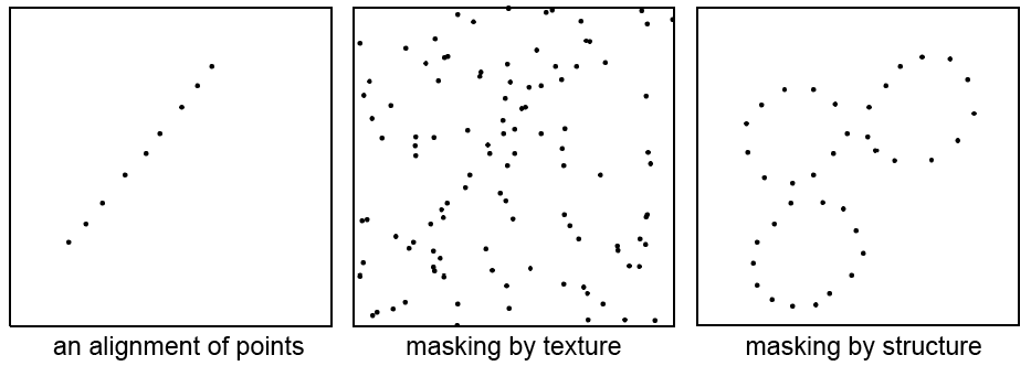
Figure 1: Exactly the same set of aligned dots is present in the three images, but it is only perceived as such in the first one. The second one is a classic masking by texture case and the third a masking by structure one, often called “Gestalt conflict”.

From a gestaltic point of view, a point alignment is a group of points sharing the property of being aligned in one direction. While it may seem a simple gestalt, Fig. 1 shows how complex the alignment event is. From a purely factual point of view, the same alignment is present in the three figures. However, it is only perceived as such by most viewers in the first one. The second and the third figures illustrate two occurrences of the masking phenomenon discovered by gestaltists kanizsa:vedere : the masking by texture, which occurs when a gestalt is surrounded by a clutter of randomly distributed similar objects or distractors, and the masking by structure, which happens when the alignment is masked by other perceptually more relevant gestalts, a phenomenon also called perceptual conflict by gestaltists metzger ; metzger:en ; kanizsa . The magic disappearance of the alignment in the second and third figures can be accounted for in two very different ways. As for the first one, we shall see that a probabilistic a contrario model DMM_book is relevant and can lead to a quantitative prediction. As for the second disappearance, it requires the intervention of another more powerful grouping law, the good continuation kanizsa1979organization .

These examples show that a mathematical definition of dot alignments is required before even starting to discuss how to detect them. A purely geometric-physical description is clearly not sufficient to account for the masking phenomenon. Indeed, an objective observer making use of a ruler would be able to state the existence of the very same alignment at the same precision on all three figures. But this statement would contradict our perception, as it would contradict any reasonable computational (definition and) theory of alignment detection.

This experiment also shows that the detection of an alignment is highly dependent on the context of the alignment. It is therefore a complex question, and must be decided by building mathematical definitions and detection algorithms, and confronting them to perception. As the patterns of Fig. 1 already suggest, simple computational definitions with increasing complexity will nevertheless find perceptual counterexamples. There is no better way to describe the ensuing “computational gestaltic game” than describing how the dialogue of more and more sophisticated alignment detection algorithms and counterexamples help build up a perception theory.

3 Basic Dot Alignment Detector

A very basic idea that could provide a quantitative context-dependent definition of dot alignments is to think of them as thin, rectangular shaped point clusters. In that case, the key measurements would be the relative dot densities inside and outside the rectangle. The algorithm described in this section follows the a contrario methodology (DMM_book, , Sect. 3.2) according to which a group of elements is detectable as a gestalt if and only if it has a low enough probability of occurring just by chance in an a contrario background model.

We shall first introduce briefly the a contrario framework DMM_book ; dmm2000 ; DMM2003 . The approach is based on the non-accidentalness principle witkin1 ; wagemans-nonaccidental ; es2003computational ; spelke1990principles (sometimes called Helmholtz principle) that states that structures are perceptually relevant only when they are unlikely to arise by accident. An alternative statement is “we do not perceive any structure in a uniform random image” (DMM_book, , p.31). The a contrario framework is a particular formalization of this principle adjusting the detection thresholds so that the expected number of accidental detections is provably bounded by a small constant $\varepsilon$. The key point is how to define accidental detections. This requires a stochastic model, the so-called a contrario model, characterizing unstructured or random data in which the sought gestalt could only be observed by chance.

Consider a dot pattern defined on a domain $D$ with total area $S_{D}$ and containing $N$ dots, see Fig. 2. We are interested in detecting groups of dots that are well aligned. A first reasonable a contrario hypothesis $H_{0}$ for this problem is to suppose that the $N$ dots are the result of a random process where points are independent and uniformly distributed in the domain. The question is then to evaluate whether the presence of aligned points contradicts the a contrario model or not.

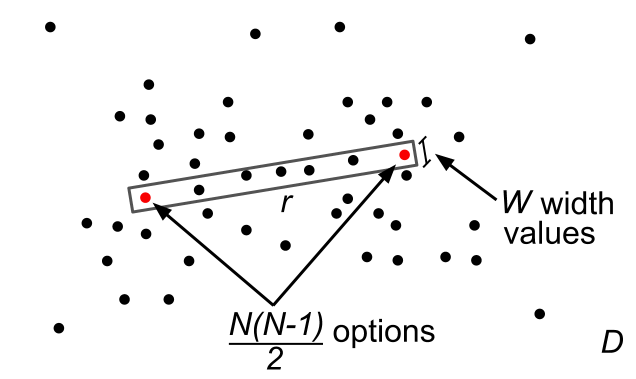
Figure 2: A schematic representation of the evaluated rectangle. In an image with $N$ points, there are $(N(N-1)\times W)/2$ possible rectangles defined by two dots. In the case shown in this figure, $N=49$ and $k(r,\mathbf{x})=5$.

Given an observed set of $N$ points $\mathbf{x}=\{x_{i}\}_{i=1\ldots N}$ and a rectangle $r$ (the candidate to contain an alignment), we will denote by $k(r,\mathbf{x})$ the number of those points observed inside $r$. We decide whether to keep this candidate or not based on two principles: a good candidate should be non-accidental, and any equivalent or better candidate should be kept as well. The degree of non-accidentalness of an observed rectangle $r$ can be measured by how small the probability $\mathds{P}\big{[}k(r,\mathbf{X})\geq k(r,\mathbf{x})\big{]}$ is, where $\mathbf{X}$ denotes a random set of $N$ dots following $H_{0}$. In the same vein, a rectangle $r^{\prime}$ will be considered at least as good as $r$ given the observation $\mathbf{x}$, if $\mathds{P}\big{[}k(r^{\prime},\mathbf{X})\geq k(r^{\prime},\mathbf{x})\big{]}\leq\mathds{P}\big{[}k(r,\mathbf{X})\geq k(r,\mathbf{x})\big{]}$.

Recall that we want to bound the expected number of accidental detections. Given that $N_{tests}$ candidates will be tested, the expected number of rectangles which are as good as $r$ under $H_{0}$, is about DMM_book

$$N_{tests}\cdot\mathds{P}\Big{[}k(r,\mathbf{X})\geq k(r,\mathbf{x})\Big{]}.$$ (1)

The $H_{0}$ stochastic model fixes the probability law of the random number of points in the rectangle, $k(r,\mathbf{X})$, which only depends on the total number of dots $N$. The discrete nature of this law implies that (1) is not actually the expected value but an upper bound of it DMM_book ; GJ08 . Let us now analyze the two factors in (1).

Here the a contrario model $H_{0}$ assumes that the $N$ points are i.i.d. with uniform density on the domain. Under the a contrario hypothesis $H_{0}$, the probability that one dot falls into the rectangle $r$ is

$$p=\frac{S_{r}}{S_{D}},$$ (2)

where $S_{r}$ is the area of the rectangle and $S_{D}$ the area of the domain. As a consequence of the independence of the random points, $k(r,\mathbf{X})$ follows a binomial distribution. Thus, the probability term $\mathds{P}\big{[}k(r,\mathbf{X})\geq k(r,\mathbf{x})\big{]}$ is given by

$$\mathds{P}\Big{[}k(r,\mathbf{X})\geq k(r,\mathbf{x})\Big{]}=\mathcal{B}\big{(}N,k(r,\mathbf{x}),p\big{)}$$ (3)

where $\mathcal{B}(n,k,p)$ is the tail of the binomial distribution

$$\mathcal{B}(n,k,p)=\sum_{j=k}^{n}\binom{n}{j}p^{j}(1-p)^{n-j}.$$ (4)

The number of tests $N_{tests}$ corresponds to the total number of rectangles that could show an alignment, which in turn is related to the number of pairs of points defining such rectangles. With a set of $N$ points this gives $\frac{N\times(N-1)}{2}$ different pairs of points.

The set of rectangle widths to be tested must be specified a priori as well. In the a contrario approach, a compromise must be found between the number of tests and the precision of the gestalts that are being sought for. The larger the number of tests, the lower the statistical relevance of detections. However, if the set of tests is chosen wisely, gestalts fitting accurately the tests will have a very low probability of occurrence under $H_{0}$ and will therefore be more significant.

At a digital image precision, the narrowest possible width for an alignment is 1 (taking the side of a pixel as length unit). The series of tested widths grows geometrically until it achieves a maximal possible width, which can be set a priori as a function of the alignment length. Since the number of tested widths depends on the length of the alignment, we cannot predict a priori (before the dots have been drawn) how many tests will be done. Fortunately the total number of widths can be estimated as the number of widths tested in an average rectangle times the number of evaluated rectangles. We call this quantity $W$. The impact of this approximation in the detector results is insignificant DMM_book . The total number of tested rectangles is then:

$$N_{tests}=\frac{N(N-1)\times W}{2}.$$ (5)

We will define now the fundamental quantity of the a contrario framework, the Number of False Alarms (NFA) associated with a rectangle $r$ and a set of dots $\mathbf{x}$:

$$\mathrm{NFA}(r,\mathbf{x})=N_{tests}\cdot\mathds{P}\Big{[}k(r,\mathbf{X})\geq k(r,\mathbf{x})\Big{]}=\frac{N(N-1)\times W}{2}\cdot\mathcal{B}\Big{(}N,k(r,\mathbf{x}),p\Big{)}.$$ (6)

This quantity corresponds, as said before (Eq. 1), to the expected number of rectangles which have a sufficient number of points to be as rare as $r$ under $H_{0}$. When the NFA associated with a rectangle is large, this means that such an event is to be expected under the a contrario model, and therefore is not relevant. On the other hand, when the NFA is small, the event is rare and probably meaningful. A perceptual threshold $\varepsilon$ must nevertheless be fixed, and rectangles with $\mathrm{NFA}(r,\mathbf{x})<\varepsilon$ will be called $\varepsilon$-meaningful rectangles es2003computational , constituting the detection result of the algorithm.

Theorem 2.1 (DMM_book ).

$$\mathds{E}\left[\sum_{R\in\mathcal{R}}\mathds{1}_{\mathrm{NFA}(R,\mathbf{X})<\varepsilon}\right]\leq\varepsilon$$

where $\mathds{E}$ is the expectation operator, $\mathds{1}$ is the indicator function, $\mathcal{R}$ is the set of rectangles considered, and $\mathbf{X}$ is a random set of points on $H_{0}$.

The theorem states that the average number of $\varepsilon$-meaningful rectangles under the a contrario model $H_{0}$ is bounded by $\varepsilon$. Thus, the number of detections in noise is controlled by $\varepsilon$ and it can be made as small as desired. In other words, this shows that our detector satisfies the non-accidentalness principle.

Following Desolneux, Moisan, and Morel dmm2000 ; DMM_book , we shall set $\varepsilon=1$ once and for all. This corresponds to accepting on average one false detection per image in the a contrario model, which is generally reasonable. Also, the detection result is not sensitive to the value of $\varepsilon$, see DMM_book .

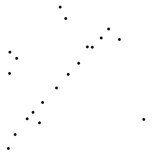
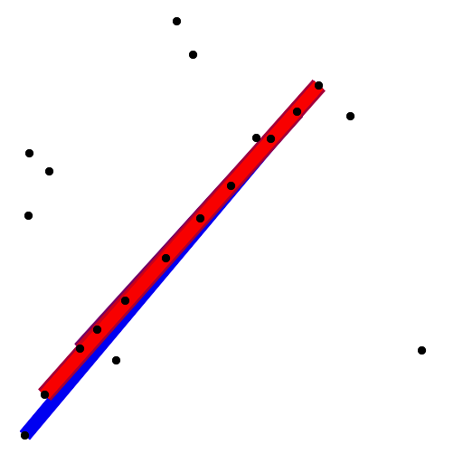
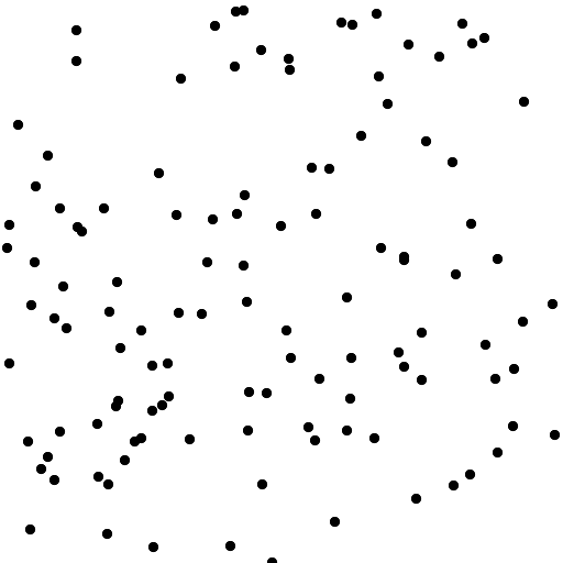
(a)	(b)		(c)	(d)

Figure 3: Results from the basic dot alignment detector. (a) and (c) are the input data, and (b) and (d) are the corresponding results. Each detection is represented by a rectangle and its color indicates the NFA value. In (b) the algorithm correctly detects the obvious alignment. Notice that multiple and redundant rectangles were detected; this problem will be discussed in Sect. 5. The data set (c) contains the same set of points in (a) plus added noise dots, thus the aligned dots are still present. However, the algorithm handles correctly the masking by texture or noise and produces no detection.

Figure 3 shows the results of the basic algorithm in two simple cases. The results are as expected: the visible alignment in the first example is detected, while no detection is produced in the second. Actually, the dots in the first example are also present in the second one, but the addition of random dots masks the alignment, in accordance with human perception. Note that the first example produces many redundant detections; this problem will be handled in Sect. 5.

4 A Refined Dot Alignment Detector

Naturally, the simple model for dot alignment detection presented in the last section does not take into account many situations that can arise and significantly affect the perception of alignments. For example: what happens if there are point clusters inside the alignment? What if the background image has a non uniform density? Should not the algorithm prefer alignments where the points are equally spaced? These questions, among others, arise when subjects play the gestaltic game and try to fool the algorithm with new drawings. There are two ways to fool the algorithm: One is by drawing a particular context that prevents the algorithms from detecting a conspicuous alignment. Inversely, the other sort of counterexample is a drawing inducing detections that remain invisible to the human eye. As more counterexamples are found, more sophisticated versions of the algorithm must be developed, and each new version will become harder to falsify than the previous one.

Using this methodology, we produced several refined versions of the basic algorithm. Here we will present the principal counterexamples that were found, and then describe the last version of the algorithm which takes all of them into account. This algorithm is therefore harder to fool. Ideally, the game should end when the Turing test pinar2000turing is satisfied, namely when a human observer will be unable to distinguish between the detections produced by a machine and by a human.

First, we noticed a deficiency in the detector when zones in the image have higher dots density. This problem arises naturally from the wrong a contrario assumption that the whole image has the same density of points. When it is not the case, the global density estimation can be misleading and produces poor detection results, as illustrated in Fig. 4 (a). The solution for this is to compute a local density estimation with respect to the evaluated rectangle. The algorithm uses a local window with size proportional to the width of the evaluated alignment.

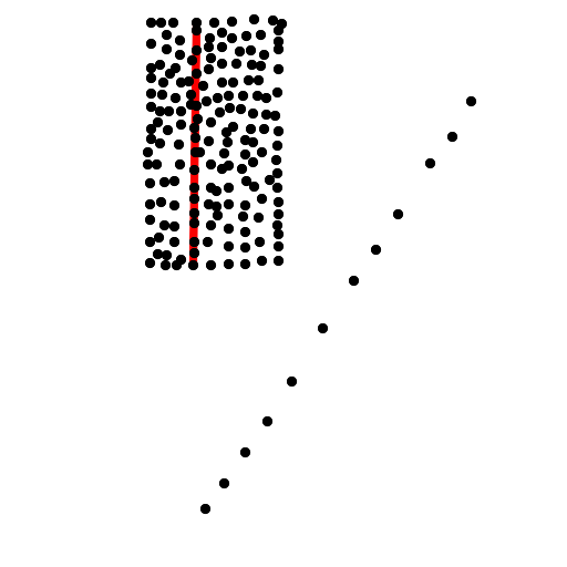
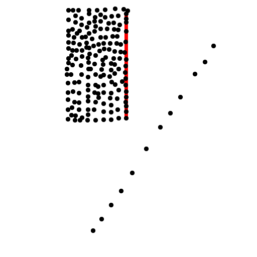
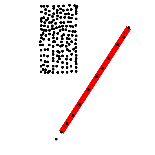
(a)	(b)	(c)

Figure 4: Local vs. global density estimation. In each example, only the most meaningful detected alignment (the one with the lowest NFA) is shown for each algorithm. The algorithms (a), (b), (c) use a background model with growing complexity to avoid wrong detections. (a) global density estimation: the detected segment is not the most meaningful for our perception, but has nevertheless a high dot density compared to the average image density used as background model. (b) here a local density estimation gives the background model, but the local density is lower on the border of the big dot rectangle, hence the detection. (c) this last problem is avoided by computing a local density estimation taking the maximum density on both sides of the alignment.

However, this local density estimation can introduce new problems such as a “border effect”, as shown in Fig. 4 (b). Indeed, the density estimation is lower on the border of the dot rectangle than inside it, because outside the rectangle there are no dots. Thus, the algorithm detects on the border a non-accidental, meaningful excess with respect to the local density.

In order to avoid this effect, the version of the algorithm used in Fig. 4 (c) measures for the background model the maximum of the densities measured on both sides of the alignment. In short, to be detected, an alignment must show a higher dot density than in both regions immediately on its left and right. This local alignment detector is therefore similar to classic second order Gabor filters where an elongated excitatory region is surrounded by two inhibitory regions. The local points estimation is calculated in the following way, see Fig. 5. The local window is divided in three parts. $R_{1}$ is the rectangle formed by the area of the local window on the left of the alignment. $R_{3}$ is the area of the local window on the right of the alignment, and $R_{2}$ is the rectangle which forms the candidate alignment. Note that the length of the local window is the same as the alignment and that we can consider any arbitrary orientation for it. Next, the algorithm counts the numbers of dots $M_{1}$, $M_{2}$, and $M_{3}$ in $R_{1}$, $R_{2}$ and $R_{3}$ respectively. Finally the a contrario model assumes that the number of dots in the local window $R_{1}\cup R_{2}\cup R_{3}$ is

$$n(r,\mathbf{x})=\max(M_{1},M_{3})\times 2+M_{2},$$ (7)

and that these dots are randomly distributed.

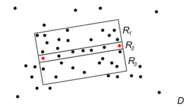
Figure 5: In the refined version of the algorithm, the density of points is measured to each side of the evaluated rectangle. The maximum of the densities in $R_{1}$ and $R_{3}$ is taken and this value is used as an estimation of the dot density in both $R_{1}$ and $R_{3}$.

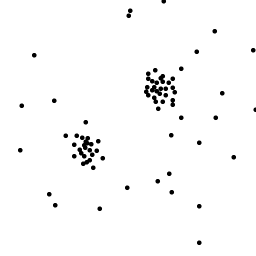
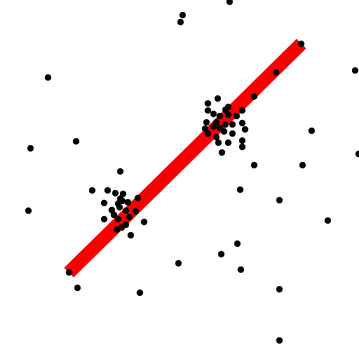
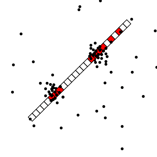
(a)	(b)	(c)

Figure 6: Counting occupied boxes to avoid false detections from the presence of clusters. The dot pattern shown in image (a) presents two dot clusters but no alignment. However, the basic algorithm finds a thin rectangle with a high dot density, hence a false detection, as shown in (b). Dividing the rectangle into boxes and counting the occupied ones, avoids this misleading cluster effect, as seen in (c), where the occupied boxes are marked in red and no alignment is actually detected.

There is still an objection to this new algorithm, obtained in the gestaltic game by introducing small dot clusters, as shown in Fig. 6 (a). The detected alignment in Fig. 6 (b) seems clearly wrong. There is indeed a meaningful dot density excess inside the red rectangle, but this excess is caused by the clusters, not by what could be termed an alignment. While the algorithm counted every point, the human perception seems to group the small clusters into a single entity, and count them only once. Also, as suggested in other studies PreissThesis ; Tripathy99 ; Uttal73 , the density is not the only property that makes an alignment perceptually meaningful; another characteristic to consider is the uniform spacing of the dots in it, which the gestaltists call the principle of constant spacing. These objections have led to a still more sophisticated version of the alignment detector. In order to take into account both issues (avoiding small clusters and favoring regular spacing) a more advanced version of the alignment detector was designed which divides each candidate rectangle into equal boxes. The algorithm counts the number of boxes that are occupied by at least one point, instead of counting the total number of points. In this way, the minimal NFA is attained when the dots are perfectly distributed along the alignment. In addition, a concentrated cluster in the alignment has no more influence on the alignment detection than a single dot in the same position.

The NFA calculation for this refined version of the algorithm is slightly different than for the basic one. The event for which we are estimating an expected number of occurrences in a background model is defined as follows. Given two points and a number of boxes $c$, the question is: What is the probability that the number of occupied boxes among the $c$ is larger than the expected number under the a contrario model? Let us start by computing the probability of one dot falling in one of the boxes:

$$p_{0}=\frac{S_{B}}{S_{L}},$$ (8)

where $S_{B}$ and $S_{L}$ are the areas of the boxes and the local window respectively. Then, the probability of having one box occupied by at least one of the $n(r,\mathbf{x})$ dots (Eq. 7) is:

$$p_{1}=\mathcal{B}\big{(}n(r,\mathbf{x}),1,p_{0}\big{)}.$$ (9)

We call occupied boxes the ones that have at least one dot inside, and we will denote by $b(r,c,\mathbf{x})$ the observed number of occupied boxes in the rectangle $r$ divided into $c$ boxes. Finally, the probability of having at least $b(r,c,\mathbf{x})$ of the $c$ boxes occupied is

$$\mathcal{B}\big{(}c,b(r,c,\mathbf{x}),p_{1}\big{)}.$$ (10)

A set $\mathcal{C}$ of different values are tried for the number of boxes $c$ into which the rectangle is divided. Thus, the number of tests needs to be multiplied by its cardinal $|\mathcal{C}|$. In practice we set $|\mathcal{C}|=\sqrt{N}$ and that leads to

$$N_{tests}=\frac{N(N-1)\times W\times|\mathcal{C}|}{2}=\frac{N(N-1)\times W\times\sqrt{N}}{2}.$$ (11)

The NFA of the new event definition is then:

$$\mathrm{NFA}(r,\mathbf{x})=\frac{N(N-1)\times W\times\sqrt{N}}{2}\cdot\min_{c\in\mathcal{C}}\mathcal{B}\big{(}c,b(r,c,\mathbf{x}),p_{1}\big{)}.$$ (12)

Figs. 4 (c) and 6 (c) show two examples of the resulting algorithm, and we will show some more after discussing the masking problem.

5 Masking

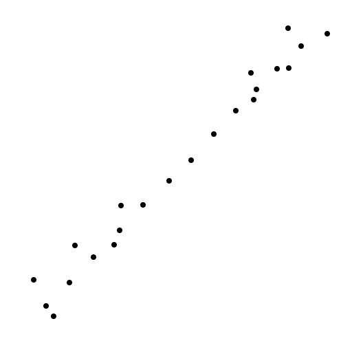
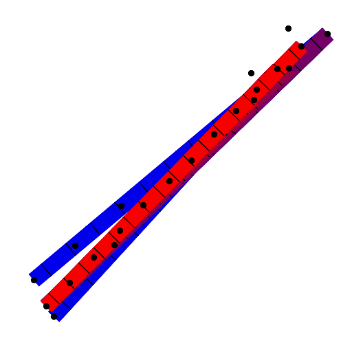
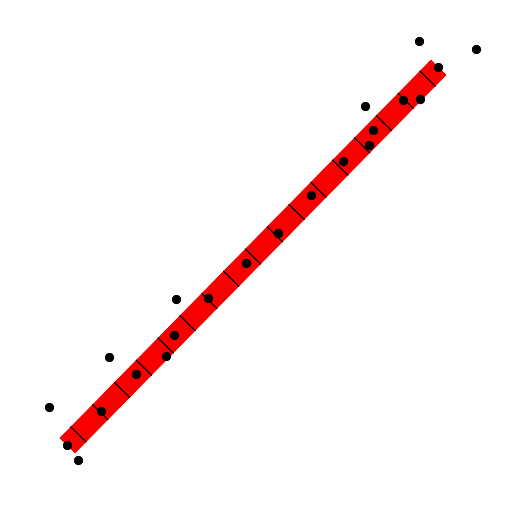
Figure 7: Redundant detections. Left: dot pattern. Center: all significant alignments found by the refined dot alignment detector described in Sect. 4. The color represents the relative NFA value, where red is the most significant (smallest NFA value) and blue the least (highest NFA value). Right: Result of the masking process.

As was observed in Fig. 3, all the described alignment detectors may produce redundant detections. The reason is that a relevant gestalt is generally formed by numerous elements and many subgroups also form relevant gestalts in the sense of the non-accidentalness principle. Every pair of dots defines a rectangle to be tested. Clearly, in a conspicuous alignment there will be many such rectangles that partially cover the main alignment and are therefore also meaningful. This redundancy phenomenon can involve dots that belong to the real alignment as well as background dots near the alignment, that can contribute to a rectangle containing a large number of dots, as illustrated in Fig. 7. However, in such cases humans perceive only one gestalt. Indeed, one could expect that there is only one causal reason leading to redundant detections and it makes sense to select the best rectangle to represent it.

A similar phenomenon is described in the Gestalt literature kanizsa:vedere . Most scenes contain other possible interpretations that are masked by the global interpretation. A simple example is shown in Fig. 8 where subsets of the grid of dots form a huge quantity of gestalts, but are invisible because they are masked by the rectangular matrix of dots. This fact is, after Vicario, called Kanizsa’s paradox DMM_book .

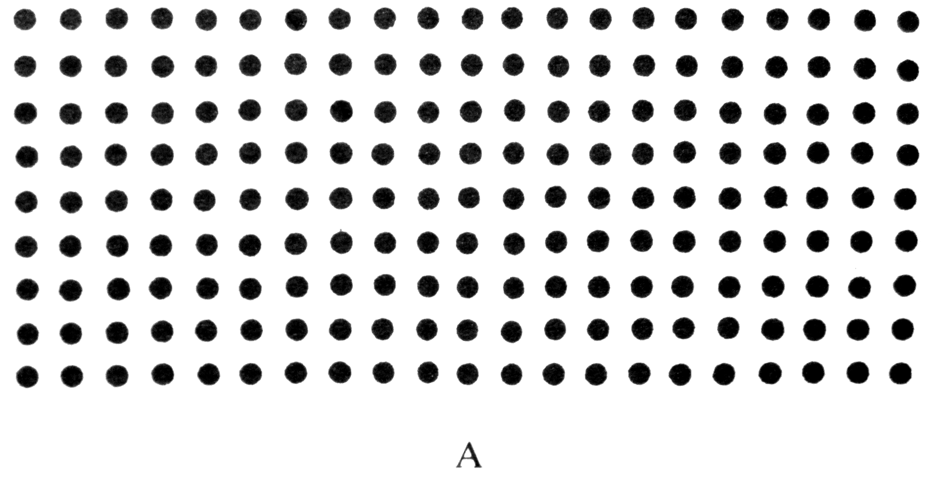
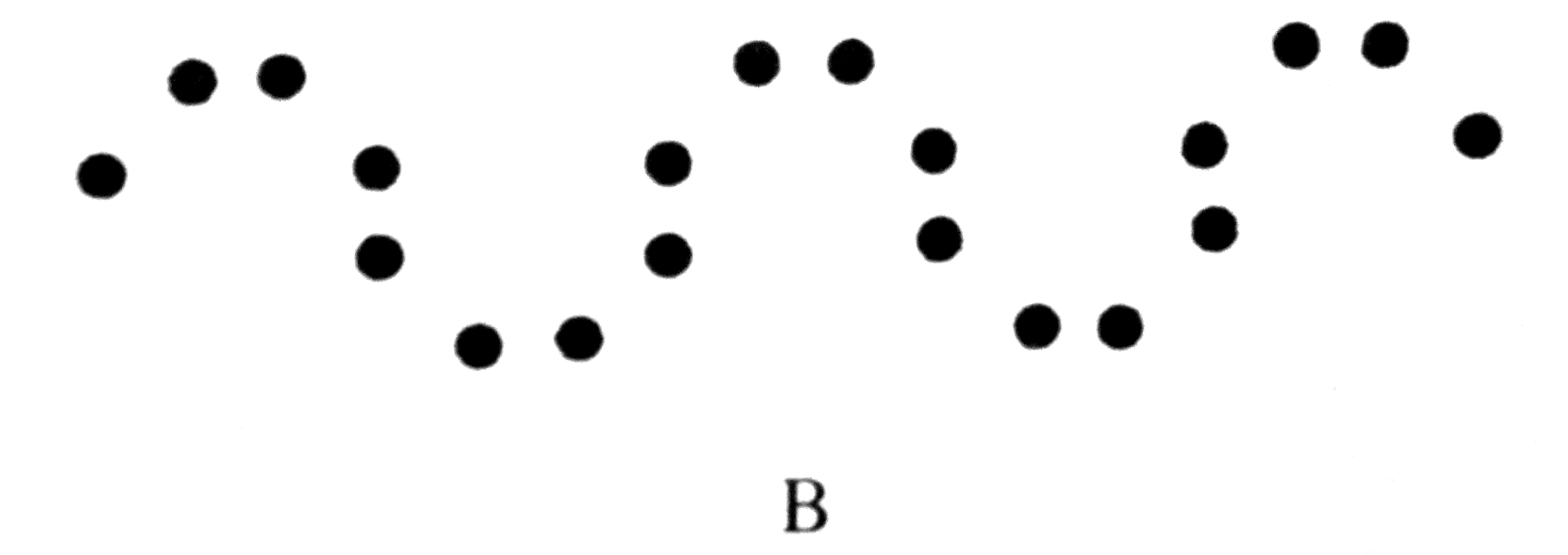
Figure 8: A masking example by Kanizsa (kanizsa:vedere, , p.155): The “curve” in B is also present in the grid of dots A; nevertheless, it is not visible as it is masked by the global matrix configuration.

A simple model for this masking process was proposed by Desolneux et al. DMM_book under the name of “exclusion principle”. The main idea is that each basic element (for example the dots) cannot contribute to more than one perceived group or gestalt. The process is as follows: The most meaningful observed gestalt (the one with smallest NFA) is kept as a valid detection. Then, all the basic elements (the dots in our case) that were part of that validated group are assigned to it and the remaining candidate gestalts cannot use them anymore. The NFA of the remaining candidates is re-computed without counting the excluded elements. In that way redundant gestalts lose most of their supporting elements and are no longer meaningful. On the other hand, a candidate that corresponds to a different gestalt keeps most or all of its supporting basic elements and remains meaningful. The most meaningful candidate among the remaining ones is then validated and the process is iterated until there are no more meaningful candidates.

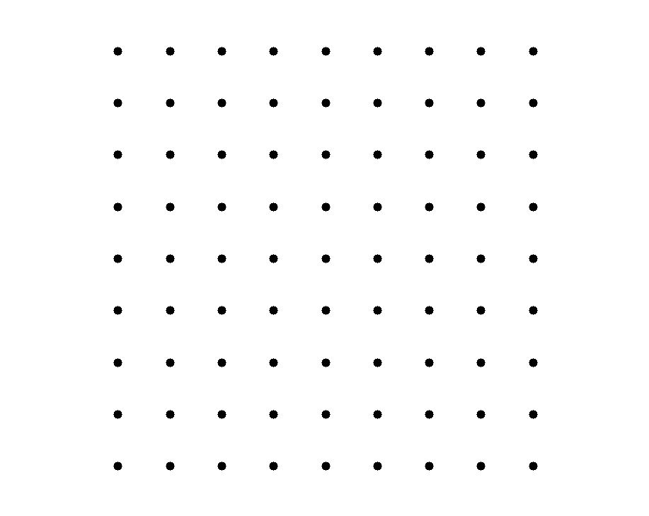
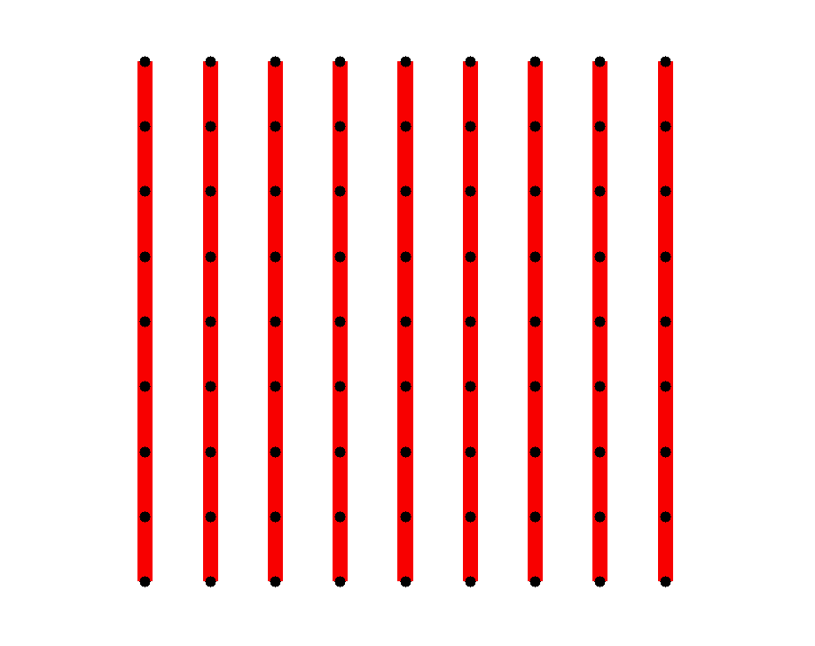
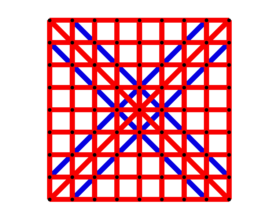
Figure 9: Examples of two alternative formulations of the masking process. Left: Set of dots. Center: The Exclusion Principle as defined in DMM_book , a validated gestalt prevents others from using its dots. The vertical alignments (that were evaluated first) mask almost all the horizontal ones. Right: The Masking Principle, described in the text, which solves the ambiguities without forbidding basic elements to participate of two different gestalts. In this example, no individual alignment can mask an individual one in another direction. Thus we get all oblique, horizontal and vertical meaningful alignments.

This formulation of the masking process often leads to good results, removing redundant detections while keeping the good ones. However, the gestaltic game showed that it may also lead to unsatisfactory results as illustrated in Fig. 9. The problem arises when various gestalts have many elements in common. As one gestalt is evaluated after the other, it may happen that all of its elements have been removed, even if the gestalt is in fact not redundant with any of the other ones. In the example of Fig. 9, individual horizontal and vertical alignments are not redundant, but if all the vertical ones have been detected first, the remaining horizontal ones will be (incorrectly) masked. This example shows a fundamental flaw of the exclusion principle: it is not sound to impose that a basic element belongs to a single perceptually valid gestalt. There must be a global explanation of the organization of the basic elements in visible gestalts which is at the same time coherent with each individual gestalt (eliminating local redundancy) and with the general explanation of the scene in such a way that some basic elements can participate of several gestalts without contradiction. The solution seems to be in a sort of relaxation of the exclusion principle. The following definitions sketch a possible solution.

Definition 2.2 (Building Elements).

We call building element any atomic image component that can be a constituent element of several gestalts. Valid examples of building elements are dots, segments, or even gestalts themselves, that can be recursively grouped in clusters or alignments. From that point of view any gestalt can be used as a building element for higher level gestalts.

Definition 2.3 (Masking Principle).

A meaningful gestalt $B$ will be said “masked by a gestalt $A$” if $B$ is no longer meaningful when evaluated without counting its building elements belonging to $A$. In such a situation, the gestalt is not retained as detected.

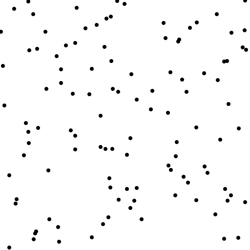
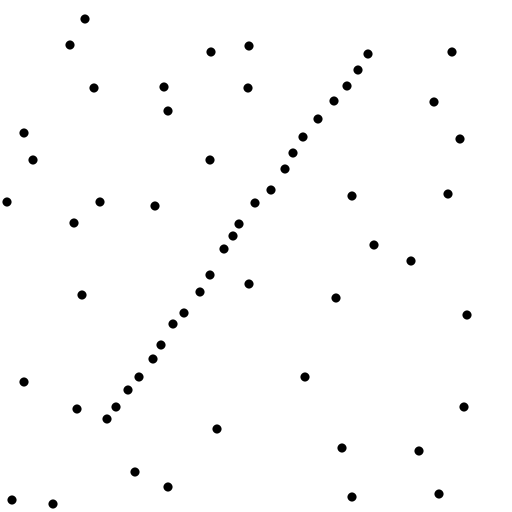
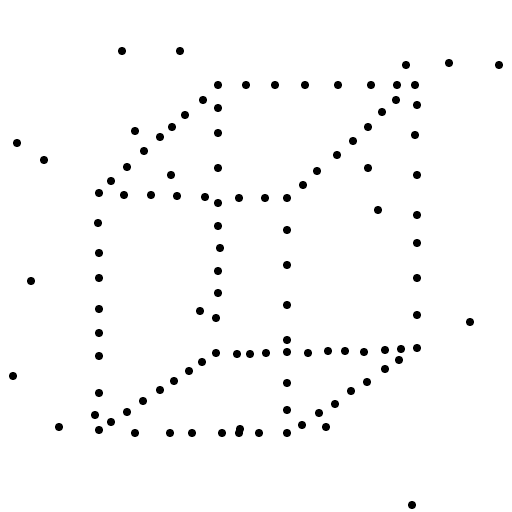
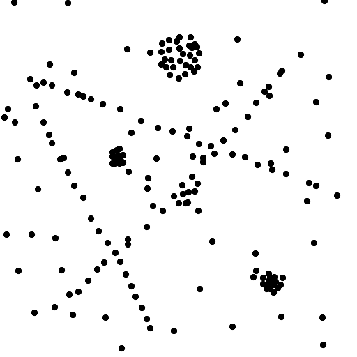
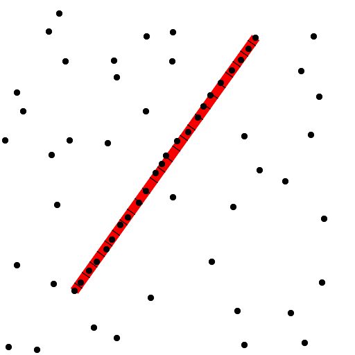
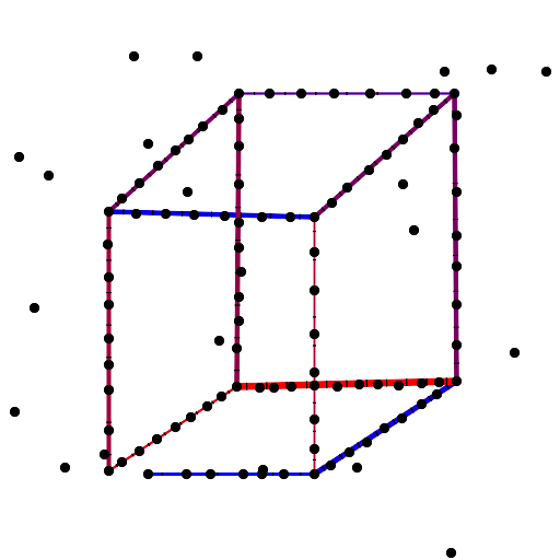
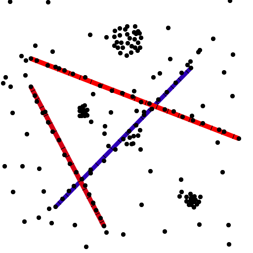
Figure 10: Results of the final dot alignment detector, using the refined method described in Sect. 4 in conjunction with the Masking Principle (Def. 2.3). The top row is the input data; the bottom row shows the results.

In short, a meaningful gestalt will be detected if it is not masked by any other detected gestalt. The difference is that here a gestalt can only be masked by another individual gestalt and not by the union of several gestalts as is possible with the exclusion principle. Thus this masking principle is analogous to a Nash equilibrium, in the sense that every gestalt remains meaningful when separately subtracting from it the building blocks of any other gestalt. A procedural way to attain this result is to validate gestalts one by one, starting by the one with smallest NFA; before accepting a new gestalt, it is checked that it is not masked by any one of the previously detected gestalts. The masking principle applies easily to point alignments.

Fig. 10 shows some dot alignment detection results when combining the method of the previous section and the masking principle. The results obtained in these examples are as expected.

6 Online Gestaltic Game

The gestaltic game allowed us to discover examples of dot arrangements that the current algorithm is not able to handle correctly. The hardest ones we encountered to date belong to the “masking by structure” kind, as those presented in the right hand part of Fig. 1. Surely there are more cases than those discovered so far. To facilitate the search we created an online interface where everyone can easily play the gestaltic game inventing new counterexamples.

Being interactive, the online gestaltic game is designed to be eventually published in the IPOL journal. It allows users to draw their own dot patterns and to see the output of the detection algorithm. Alternatively, the user can upload a set of dots, or modify an existing one by adding or removing individual dots or adding random dots. All the experiments are stored and accessible in the “archive” part of the site and may help improve the theory.

Current work is focused on the conflict between different gestalts with the objective of handling the masking by structure problem.

3 Detection Theory versus Psychophysics

In this second part we leave the question of a quantitative gestaltism and go back to more classic psychophysics. The question is whether a quantitative framework like the a contrario detection theory can also become a useful addition for human contour perception psychophysical experiments.

Arrays of Gabor patches have become a classic tool for the study of the influence of good continuation in perceptual grouping Field93ContourIntegration ; Nygard09orientation_jitter_motion . Gabor functions ensure a control on the stimuli spectral complexity and on the spatial scale of the contours. They give a flexible and easy way for building a great variety of stimuli. It has been verified that the more aligned the Gabor patches are to the contour they lie on, the easier their perceptual grouping into a shape’s outline Field93ContourIntegration ; Nygard09orientation_jitter_motion . Fig. 11 (left), shows an easy example where most subjects recognize a bottle. But the more freedom is left to the Gabor orientation, the harder it is to distinguish such contours from the background. For the influence of other perturbations of the contour such as its motion or its curvature on the object’s identifiability, we refer to a recent study Nygard09orientation_jitter_motion .

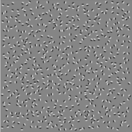
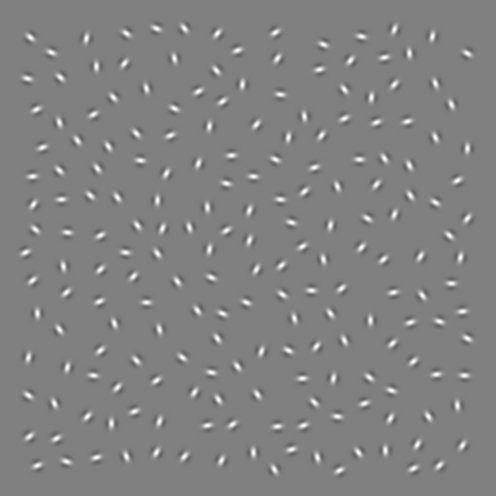
Figure 11: Left: An image extracted from Nygård et al. Nygard09orientation_jitter_motion . Right: Example of an alignment detection experiment to be developed here.

Can we hope for a quantitative interpretation to this experimental framework, namely a function of the stimuli parameters that would predict and explain the evolution of the detection performance? Probabilistic approaches (mainly Bayesian) exist for contour modeling from a perceptual point of view Attneave54InformationalAspects ; Feldman05InfoAlongContours , and have sometimes been compared experimentally to human visual perception Feldman01BayesianContour ; but none of these approaches proposed to compute a priori detection thresholds as functions of the stimuli parameters.

The influence of experimental factors such as the length of the alignment, the density of the patches, and the angular accuracy on human detection is a classic subject of psychophysical inquiry. But the question of whether human performance can be measured with only one adequate quantitative function of the parameters is still open. We shall explore here if the NFA furnished by the a contrario theory can play this role. Indeed, the NFA retains the remarkable property of being a scalar function of the three psychophysical parameters generally used in this kind of detection experiment. In classic experimental settings, these parameters are varied separately and independently, and no synthetic conclusion can be drawn; only separate conclusions on the influence of each parameter can be reached. If a function like the NFA could play the role of generic detectability parameter, the experimental parameters could for example be made to vary simultaneously in the very same experiment. In short, if the hypothesis of a single underlying detection parameter is validated, this would simplify the experimental setups and entail a new sort of quantitative analysis of the results, two stimuli being a priori considered as equivalent in difficulty if their NFA are similar.

The underlying hypothesis, that the reaction of the subjects to varying stimuli might be predicted as a single scalar function of the stimulus’ parameters, is equivalent to the classic hypothesis of a “single mechanism” for contour detection. More precisely, we shall explore if this single mechanism might obey the non-accidentalness principle (the NFA being its probabilistic quantitative expression).

To keep the line of the previous section, this study will again focus on the same simple gestalt: straight contours, that is to say alignments of Gabor elements, as illustrated in Fig. 11 (right). The remainder of this section describes the patterns used, the a contrario method, the experiment performed on humans, and the result of the comparison.

1 The Patterns

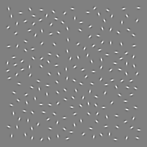
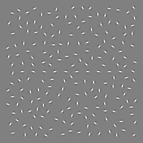
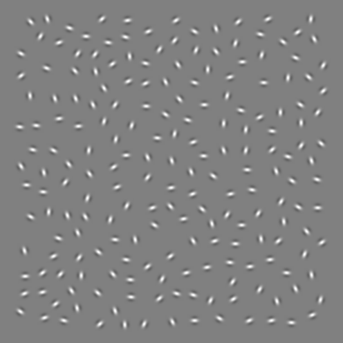
(a)	(b)	(c)

Figure 12: Three examples of stimuli used in our experiments. (a) A jitter-free alignment with 10 elements. (b) A weakly jittered alignment with 10 elements. (c) A stimulus with no alignment, containing only elements with random orientations.

Figure 12 shows three examples of the stimuli used in our experiments. All of them consist of symmetric Gabor elements with varying positions and orientations placed over a gray background. There are two kinds of stimuli: positive stimuli and negative stimuli. Negative stimuli contain elements with random orientations sampled in $[0,\pi)$, e.g. Fig. 12 (c). Positive stimuli, see Fig. 12 (a) and (b), contain a majority of random elements like in negative stimuli but also a small set of foreground elements. The latter lie on a straight line and are uniformly spaced; their orientations are randomly and uniformly sampled from an interval centered on the alignment direction. The size of this interval gives a measure of the angular jitter and will be noted by $J$. When the jitter is zero, the foreground elements have the exact same orientation as their supporting line. Inversely, a jitter of $\pi$ leads to completely isotropic elements.

The experiment is designed to study how angular jitter affects visibility. Yet, a natural question arises about the contribution to the detection of the accuracy of the alignment and of the regular spacing of the aligned elements. All the stimuli presented in this section were generated with the software GERT (v1.1) that includes special algorithms for the generation of random placed and oriented Gabor elements that mask as much as possible the aligned Gabor elements structure Demeyer11displays_using_GERT . Figure 13 shows an example displaying only the elements position; even if there is in fact a set of perfectly regularly aligned dots, it is very hard to spot them. This suggests that the position of the elements carries few useful cues about the alignment.

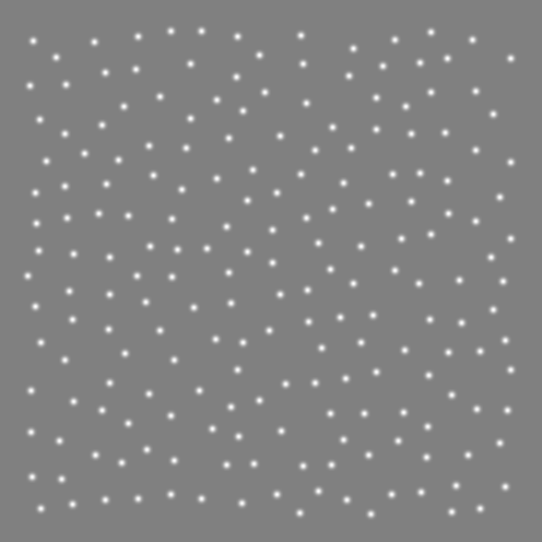
Figure 13: Influence of stimuli position. Each dot represents the position where a Gabor element will be placed. The figure includes a perfectly regular and aligned set of dots, surrounded by random placed elements, all generated by the GERT package. It is very difficult to find the alignment, which shows that the position of the elements by itself conveys few cues about the presence of the alignment. (For a comparison, see the same stimulus with Gabor elements, Fig. 11 (right), where the alignment is easily spotted.)

2 The Detection Algorithm

Let us now present the alignment detection algorithm that will be matched to human perception. The input to the algorithm is a set of Gabor elements $\mathbf{g}=\{(x_{i},\theta_{i})\}_{i=1\ldots N}$, defined by the position and orientation of each element. We will further assume that the total number of elements is a fixed quantity $N$.

A candidate to alignment is defined as a rectangle $r$, see Fig. 14 (left), and the orientation of the Gabor elements inside it will determine whether the candidate is evaluated as a valid alignment or not. The orientation of each Gabor element is compared to the one of the rectangle and when the difference is smaller than a given tolerance threshold $\tau$, the element is said to be $\tau$-aligned, see Fig. 14 (right). Two quantities will be observed for each rectangle $r$: the total number of Gabor elements inside it, $n(r,\mathbf{g})$, and the number among them that are $\tau$-aligned, $k_{\tau}(r,\mathbf{g})$. The a contrario validation is analogue to the one described in Sect. 3.

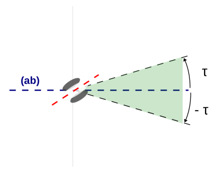
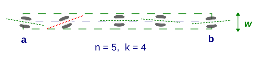
Figure 14: Left: A candidate to alignment, defined by a rectangle $R$. Right-Top: A Gabor element whose angle with $(ab)$ is larger than $\tau$ and thus it is not counted as an aligned point. Right-Bottom: A detailed example where we see a total of five Gabor elements inside the rectangle, $n(r,\mathbf{g})=5$, being $\tau$-aligned with $(ab)$, i.e. $k_{\tau}(r,\mathbf{g})=4$.

Due to the way the patterns are generated, the only relevant information to evaluate in an alignment is the orientation of the Gabor elements. Consequently, the a contrario model $H_{0}$ is defined with $N$ random variables corresponding to the orientation of the elements and satisfying the following two conditions:

• the orientations $\Theta_{i}$ are independent from each other;

• each orientation $\Theta_{i}$ follows a uniform distribution in $[0,\pi)$.

Under these a contrario assumptions, the probability that a Gabor element be $\tau$-aligned to a given rectangle is given by

$$p(\tau)=\frac{2\tau}{\pi}.$$ (13)

Notice that the symmetric Gabor elements are unaltered by a rotation of $\pi$ rads. The independence hypothesis implies that the probability term $\mathds{P}[k_{\tau}(r,\mathbf{G})\geq k_{\tau}(r,\mathbf{g})]$, where $\mathbf{G}$ is a random set of Gabor elements following $H_{0}$, is given by

$$\mathds{P}\big{[}k_{\tau}(r,\mathbf{G})\geq k_{\tau}(r,\mathbf{g})\big{]}=\mathcal{B}\Big{(}n(r,\mathbf{g}),k_{\tau}(r,\mathbf{g}),p(\tau)\Big{)},$$ (14)

where as before $\mathcal{B}(n,k,p)$ is the tail of the binomial distribution.

We still need to specify the family of tests to be performed. Each pair of dots will define a rectangle of fixed width $w$, so the total number of rectangles is $\frac{N(N-1)}{2}$. Also, a finite number of angular precisions $\tau_{i}$ will be tested for each rectangle. Then,

$$N_{tests}=\frac{N(N-1)}{2}\cdot\#\mathcal{T},$$ (15)

where $\#\mathcal{T}$ is the cardinality of the set $\mathcal{T}$ of precisions. The NFA of a candidate is defined by

$$\mathrm{NFA}(r,\mathbf{g})=N_{tests}\cdot\min_{\tau\in\mathcal{T}}\mathcal{B}\Big{(}n(r,\mathbf{g}),k_{\tau}(r,\mathbf{g}),p(\tau)\Big{)}.$$ (16)

A large NFA value corresponds to a likely (and therefore insignificant) configuration in the a contrario model; inversely, a small NFA value indicates a rare and interesting event. The proposed detection method validates a rectangle candidate $r$ whenever $\mathrm{NFA}(r,\mathbf{x})<\varepsilon$. The following theorem shows that it satisfies the non-accidentalness principle.

Theorem 3.1.

$$\mathds{E}\left[\sum_{R\in\mathcal{R}}\mathds{1}_{\mathrm{NFA}(R,\mathbf{G})<\varepsilon}\right]\leq\varepsilon.$$

where $\mathds{E}$ is the expectation operator, $\mathds{1}$ is the indicator function, $\mathcal{R}$ is the set of rectangles considered, and $\mathbf{G}$ is a random set of Gabor elements on $H_{0}$.

Once again we follow Desolneux et al. dmm2000 ; DMM_book and set $\varepsilon=1$. In our experiments, we use the NFA as an indication of the visibility of the gestalt according to the proposed theory; a value considerably smaller than 1 is “non-accidental” and should imply a conspicuous gestalt. A value larger than 1 can occur just by chance and should therefore be associated to an irrelevant gestalt. Figure 15 shows two examples of detection by this method.

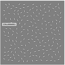
	$\mathrm{NFA}=99.5$	no detection
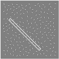
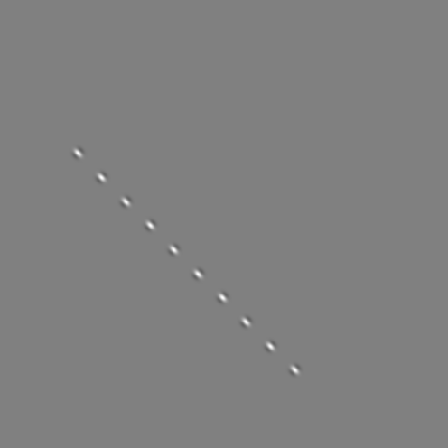
	$\mathrm{NFA}=10^{-5}$	detection

Figure 15: Two examples of the proposed validation method for alignment of Gabor elements. The rectangle in the first row has three elements inside, all of them aligned; that number is nevertheless too small to produce a detection, as its NFA value is larger than one. In the second example, all ten Gabor elements are aligned, giving an NFA of $10^{-5}$ and producing a detection.

3 Experiment

A psychophysical experiment was performed online by voluntary subjects using an interactive web site. Their task was to report on the visibility of the aligned Gabor patterns. The online methodology was necessarily more flexible and less controlled on various aspects than it would be in a laboratory: we had no reliable information about the subjects, their visualization conditions in front of their computers were not controlled, the comprehension of the task by the subjects might vary, etc. Notwithstanding their uncontrolled essence, online experiments give access to a larger number of subjects and bring a great experimental flexibility.

The data set used for this experiment is composed of over 14000 stimuli (negative and positive) as the one described in Sect. 1. Each image has a size of $496\times 496$ pixels and containing $N=200$ elements. For positive stimuli, 9 levels of jitter ($J\in\{0,\frac{\pi}{5},\frac{\pi}{4},\frac{\pi}{3},\frac{\pi}{2},\frac{2\pi}{3},\frac{3\pi}{4},\frac{4\pi}{5},\pi\}$) and 8 different segment lengths were used, between 3 and 10 elements. During each session, the subject saw 35 of these images, one after another. The first five images were training stimuli and no results were recorded at this stage of the experiment. The following 30 images were randomly sampled over the data set, with constraints that ensured a balance between negative, positive, hard and easy stimuli. For each stimulus, the subject was asked to answer whether they saw or not a “straight line”; the answer and response time were recorded. There was no time limit to provide the answer but it was suggested to answer as soon as the subject made up their mind. At the end of the session, a feedback was given on false detections and on the consistency of the subject’s answer through an “attention score”. This score rewarded the fact that the subject answered better on easy stimuli than on hard ones and indicated if the task was well understood or not.

4 Results

In order to compare human and machine perception we precomputed the NFA for each rectangle on all the images of the data set. Each image was associated to its best (smallest) NFA. The hypothesis to be tested was that the NFA value should be related directly to the visibility by humans; if this is true, the average score given to an image by humans, namely the proportion of “Yes”, should be related to the NFA of the most salient structure. In what follows we will analyze the data obtained from 7137 trials.

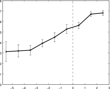
Figure 16: Comparison of the subjects’ responses to the NFA. Left: The average answer rate is plotted relative to $\log_{10}(\mathrm{NFA})$. Each point indicates the proportion of positive answers to stimuli with best NFA in the corresponding bin. Right: The average response times in seconds per bin. In both cases, the abscissa represents the scale of $\log_{10}(\mathrm{NFA})$ divided into 9 bins; the first bin is defined by $\log_{10}(\mathrm{NFA})<-5$, the last one by $\log_{10}(\mathrm{NFA})\geq 2$, and the other 7 bins by $k\leq\log_{10}(\mathrm{NFA})<k+1$ for $k=-5,\dots,1$. The error bars give approximately 95 % confidence about the mean values (each interval is defined as $[\overline{x}-2\frac{s}{\sqrt{n}},\overline{x}+2\frac{s}{\sqrt{n}}]$, where $\overline{x},s$ and $n$ are respectively the mean, standard deviation and number of trials of the bin).

The NFA scale was divided into bins. To each bin were associated statistics on the trials whose NFAs belonged to this bin. Figure 16 shows the average answer rate and response times for nine $\log_{10}(\mathrm{NFA})$ intervals. Note that $\mathrm{NFA}<1$ (or $\log_{10}(\mathrm{NFA})<0$) means detection of the alignment by the algorithm.

The results significantly support the hypothesis that a single scalar function of all parameters predicts the detectability. Indeed, the answer rate follows a sigmoid shape roughly centered at $\log_{10}(\mathrm{NFA})=0$. The second graph, plotting the response time versus the NFA, also agrees with the hypothesis: the less visible the stimuli are, the more time is spent searching for valid gestalts. Statistical tests confirm this average tendency.

The experiment confirms the hypothesis that, at least in this restricted perceptual environment (formed of three parameters, the number of Gabor patches, the length of the alignment and its jitter on orientation), the value of NFA may account for the human “detectability” of an alignment. Surprisingly, the human detection (attentive) threshold is close to the best algorithm in this restricted environment. Indeed, alignments with NFA smaller than 1 were detected by a majority of subjects. Alignments with NFA larger than one, which are likely to occur just by chance, were detected by a minority of subjects. Furthermore, the detection curve is steepest when the NFA crosses 1. The curve is not as steep for the mean response time as a function of NFA. This can be simply explained by the fact that the patience of subjects undergoes a rapid temporal erosion; they are not ready to look long for a needle in a haystack.

5 Consequence: An Online Game

Online experimentation opens new possibilities that need to be explored farther, and in particular the use of computer games as an experimentation tool. A successful game may attract the attention of subjects and if the resulting mass of results is large enough, it could compensate for the lack of control on other aspects of the experimental setting.

The player of a computer game is usually directed toward an objective and faced with obstacles. To be attractive, a game cannot be too easy, but not too hard either; a good balance of this difficulty is the key to the popularity of the game. To use games for psychophysical purposes, the player should be directed to detect some pattern, the obstacles being the conditions that preclude this perception. Motivated players will do their best effort, revealing the limits of human perception.

To go in this direction we created a prototype version of an alignment game. The player is presented with Gabor stimuli as described before. Only positive stimuli with variable difficulties are used. In this way one knows that there is an alignment gestalt; but its position is unknown and the assignment of the player is to spot it. The subject is asked to click in the image on any point of the straight line. The distance between the clicked point and the actual line segment is recorded and a score over 100 is computed as a function of this distance (the closer to the segment, the better the score). When the stimulus is quite visible, all subjects are able to point correctly to it; when it is not, the distance to the alignment becomes random. This rash transition should permit to pinpoint the human detection threshold.

The presentation of the stimuli is divided into several sequences of ten images. The first sequence is always supposed to be very easy (long segments with little jitter). Then the difficulty of the following sequences change according to the performance achieved on the previous one. The collected data will permit us to compare a detection method to human performance in the way described before. The game is still in a prototype phase but readers are invited to try it and provide feedback.

4 Conclusion

Needless to be said, the experimental devices and first results that we just described are not sufficient to make any rash conclusion on the existence of quantitative predictions of human perception. They will need to be extended to other gestalts commonly used in psychophysics, such as for example contours (good continuation), clusters, or symmetries. In the same way, the first described gestaltic game does not furnish an end algorithm modeling what we could call the human notion of alignment. Finally, we did not deliver a detection algorithm directly usable on any image, as required by the computer vision methodology. In short, this is work in progress, and our goal was to raise the attention of psychophysical researchers and computer scientists on the interest of introducing Turing tests in their methodology.

References

- (1) Ahuja, N., Tuceryan, M.: Extraction of early perceptual structure in dot patterns: integrating region, boundary, and component gestalt. Comput. Vision Graph. Image Process. 48(3), 304–356 (1989)
- (2) Attneave, F.: Some informational aspects of visual perception. Psychological Review 61(3), 183–193 (1954)
- (3) Demeyer, M., Machilsen, B.: The construction of perceptual grouping displays using GERT. Behavior Research Methods, online first. pp. 1–8 (2011)
- (4) Desolneux, A., Moisan, L., Morel, J.: Meaningful alignments. International Journal of Computer Vision 40(1), 7–23 (2000)
- (5) Desolneux, A., Moisan, L., Morel, J.: Computational gestalts and perception thresholds. Journal of Physiology - Paris 97, 311–324 (2003)
- (6) Desolneux, A., Moisan, L., Morel, J.: A grouping principle and four applications. IEEE Transactions on Pattern Analysis and Machine Intelligence (2003)
- (7) Desolneux, A., Moisan, L., Morel, J.: From Gestalt Theory to Image Analysis, a Probabilistic Approach, Interdisciplinary Applied Mathematics, vol. 34. Springer (2008)
- (8) Ellis, W. (ed.): A Source Book of Gestalt Psychology. Humanities Press (1967 (originally 1938))
- (9) Feldman, J.: Regularity-based perceptual grouping. Computational Intelligence 13(4), 582–623 (1997)
- (10) Feldman, J.: Bayesian contour integration. Attention, Perception, & Psychophysics 63, 1171–1182 (2001)
- (11) Feldman, J., Singh, M.: Information along contours and object boundaries. Psychological Review 112(1), 243–252 (2005)
- (12) Field, D.J., Hayes, A., Hess, R.F.: Contour integration by the human visual system: Evidence for a local “association field”. Vision Research 33(2), 173 – 193 (1993)
- (13) Fleuret, F., Li, T., Dubout, C., Wampler, E.K., Yantis, S., Geman, D.: Comparing machines and humans on a visual categorization test. Proceedings of the National Academy of Sciences 108(43), 17,621–17,625 (2011)
- (14) Grompone von Gioi, R., Jakubowicz, J.: On computational Gestalt detection thresholds. Journal of Physiology – Paris 103(1-2), 4–17 (2009)
- (15) Grossberg, S., Mingolla, E.: Neural dynamics of perceptual grouping: Textures, boundaries, and emergent segmentations. Attention, Perception, & Psychophysics 38(2), 141–171 (1985)
- (16) Han, F., Zhu, S.C.: Bottom-up/top-down image parsing with attribute grammar. IEEE Transactions on Pattern Analysis and Machine Intelligence 31(1), 59–73 (2009)
- (17) Kanizsa, G.: Organization in vision: Essays on Gestalt perception. Praeger New York: (1979)
- (18) Kanizsa, G.: Grammatica del vedere. Il Mulino (1980)
- (19) Kanizsa, G.: Vedere e pensare. Il Mulino (1991)
- (20) Kersten, D., Mamassian, P., Yuille, A.: Object perception as bayesian inference. Annual Review of Psychology 55(1), 271–304 (2004)
- (21) Köhler, W.: Gestalt Psychology. Liveright (1947)
- (22) Leclerc, Y.: Constructing simple stable descriptions for image partitioning. International journal of computer vision 3(1), 73–102 (1989)
- (23) Lowe, D.: Perceptual Organization and Visual Recognition. Kluwer Academic Publishers (1985)
- (24) Marr, D.: Vision. Freeman and co. (1982)
- (25) Metzger, W.: Gesetze des Sehens, third edn. Verlag Waldemar Kramer, Frankfurt am Main (1975)
- (26) Metzger, W.: Laws of Seeing. The MIT Press (2006 (originally 1936)). English translation of the first edition of metzger .
- (27) Mumford, D.: Pattern theory: the mathematics of perception. Proceedings of the International Congress of Mathematicians, Beijing I, 401–422 (2002)
- (28) Nygård, G., Van Looy, T., Wagemans, J.: The influence of orientation jitter and motion on contour saliency and object identification. Vision Research 49, 2475–2484 (2009)
- (29) Pinar Saygin, A., Cicekli, I., Akman, V.: Turing test: 50 years later. Minds and Machines 10(4), 463–518 (2000)
- (30) Preiss, K.: A theoretical and computational investigation into aspects of human visual perception: Proximity and transformations in pattern detection and discrimination. Ph.D. thesis, University of Adelaide (2006)
- (31) Sarkar, S., Boyer, K.L.: Perceptual organization in computer vision: A review and a proposal for a classificatory structure. IEEE Transactions on Systems, Man, and Cybernetics 23(2), 382–399 (1993)
- (32) Spelke, E.: Principles of object perception. Cognitive science 14(1), 29–56 (1990)
- (33) Stevens, S.: Psychophysics. Transaction Publishers (1986)
- (34) Tripathy, S.P., Mussap, A.J., Barlow, H.B.: Detecting collinear dots in noise. Vision Research 39(25), 4161 – 4171 (1999)
- (35) Turing, A.: Computing machinery and intelligence. Mind 59, 433–460 (1950)
- (36) Uttal, W., Bunnell, L., Corwin, S.: On the detectability of straight lines in visual noise: An extension of french’s paradigm into the millisecond domain. Perception and Psychophysics 8, 385–388 (1970)
- (37) Uttal, W.R.: The effect of deviations from linearity on the detection of dotted line patterns. Vision Res 13(11), 2155–63 (1973)
- (38) Vanegas, M.C., Bloch, I., Inglada, J.: Detection of aligned objects for high resolution image understanding. In: IGARSS, pp. 464–467 (2010)
- (39) Wagemans, J.: Perceptual use of nonaccidental properties. Canadian Journal of Psychology 46(2), 236–279 (1992)
- (40) Wagemans, J., Elder, J.H., Kubovy, M., Palmer, S.E., Peterson, M.A., Singh, M., von der Heydt, R.: A century of Gestalt psychology in visual perception: I. Perceptual grouping and figure–ground organization. Psychological bulletin 138(6), 1172–1217 (2012). 10.1037/a0029333
- (41) Wagemans, J., Feldman, J., Gepshtein, S., Kimchi, R., Pomerantz, J.R., van der Helm, P.A., van Leeuwen, C.: A century of Gestalt psychology in visual perception: II. Conceptual and theoretical foundations. Psychological Bulletin (2012)
- (42) Wertheimer, M.: Untersuchungen zur Lehre von der Gestalt. II. Psychologische Forschung 4(1), 301–350 (1923). An abridged translation to English is included in source-book .
- (43) Witkin, A.P., Tenenbaum, J.M.: On the role of structure in vision. In: J. Beck, B. Hope, A. Rosenfeld (eds.) Human and Machine Vision, pp. 481–543. Academic Press (1983)
- (44) Witkin, A.P., Tenenbaum, J.M.: What is perceptual organization for? IJCAI-83 2, 1023–1026 (1983)
- (45) Zhu, S., Yuille, A.: Region competition: Unifying snakes, region growing, and bayes/mdl for multiband image segmentation. Pattern Analysis and Machine Intelligence, IEEE Transactions on 18(9), 884–900 (1996)
- (46) Zhu, S.C., Mumford, D.: A stochastic grammar of images. Foundations and Trends in Computer Graphics and Vision 2(4), 259–362 (2006)