On the Estimation of Entropy in the FastICA Algorithm

Abstract

The fastICA method is a popular dimension reduction technique used to reveal patterns in data. Here we show both theoretically and in practice that the approximations used in fastICA can result in patterns not being successfully recognised. We demonstrate this problem using a two-dimensional example where a clear structure is immediately visible to the naked eye, but where the projection chosen by fastICA fails to reveal this structure. This implies that care is needed when applying fastICA. We discuss how the problem arises and how it is intrinsically connected to the approximations that form the basis of the computational efficiency of fastICA.

Keywords – Independent component analysis, fastICA, projections, projection pursuit, blind source separation, counterexample, convergence, approximation

2010 AMS subject classification: 62-04, 65C60

1 Introduction

Independent Component Analysis (ICA) is a well-established and popular dimension reduction technique that finds an orthogonal projection of data onto a lower-dimensional space, while preserving some of the original structure. ICA is also used as a method for blind source separation and is closely connected to projection pursuit. We refer the reader to Hyvärinen et al. (2004), Hyvärinen (1999) and Stone (2004) for a comprehensive overview of the mathematical principles underlying ICA and its applications in a wide variety of practical examples.

In ICA, the projections that are determined to be “interesting” are those that maximise the non-Gaussianity of the data, which can be measured in several ways. One quantity for this measurement that is used frequently in the ICA literature is entropy. For distributions with a given variance, the Gaussian distribution is the one which maximises entropy, and all other distributions have strictly smaller entropy. Therefore, our aim is to find projections which minimise the entropy of the projected data. Different methods are available for both the estimation of entropy and the optimisation procedure, and have different speed-accuracy trade-offs.

A widely used method to perform ICA in higher dimensions is fastICA (Hyvärinen and Oja, 2000). This method has found applications in areas as wide ranging as facial recognition (Draper et al., 2003), epileptic seizure detection (Yang et al., 2015) and fault detection in wind turbines (Farhat et al., 2017). Recent works on extensions of the algorithm can be seen in Miettinen et al. (2014), Ghaffarian and Ghaffarian (2014) and He et al. (2017). The fastICA method uses a series of substitutions and approximations of the projected density and its entropy. It then applies an iterative scheme for optimising the resulting contrast function (which is an approximation to negentropy). Because of its popularity in many areas, analysis and evaluation of the strengths and weaknesses of the fastICA algorithm is crucially important. In particular, we need to understand both how well the contrast function estimates entropy and the performance of the optimisation procedure.

The main strength of the fastICA method is its speed, which is considerably higher than many other methods. Furthermore, if the data is a mixture of a small number of underlying factors, fastICA is often able to correctly identify these factors. However, fastICA also has some drawbacks, which have been pointed out in the literature. Learned-Miller and Fisher III (2003) use test problems from Bach and Jordan (2002) with performance measured by the Amari error (Amari et al., 1996) to compare fastICA to other ICA methods. They find that these perform better than fastICA on many examples. Focussing on a different aspect, Wei (2014) investigates issues with the convergence of the iterative scheme employed by fastICA to optimise the contrast function. In Wei (2017) it is shown that the two most common fastICA contrast functions fail to de-mix certain bimodal distributions with Gaussian mixtures, although some other contrast function choices (related to classical kurtosis estimation) may give reliable results within the fastICA framework.

In this article we identify and discuss a more fundamental problem with fastICA. We demonstrate that the approximations used in fastICA can lead to a contrast function where the optimal points no longer correspond to directions of low entropy.

Fig. 1: Scatter plot of original data with densities of the projected data in the direction obtained by $m$-spacing ICA (solid line) and fastICA (dotted line). Kernel density estimation was used to obtain the marginal densities shown.

To illustrate the effect discussed in this paper, we consider the example shown in Figure 1. In this example, two-dimensional samples are generated from a two-dimensional normal distribution, conditioned on avoiding a collection of parallel bands (see Section 5 for details). This procedure produces a pattern which is obvious to the bare eye, and indeed the projection which minimises entropy (solid lines) exposes this pattern. In contrast, the fastICA contrast function seems unable to resolve the pattern of bands and prefers a direction with higher entropy which does not expose the obvious pattern (dotted lines).

We remark that this failure by fastICA to recover the obvious structure is relatively robust in this example. Changing the parameters used in the fastICA method does not significantly change the outcome, and the underlying structure is still lost. It is also worth mentioning here that the example dataset was very simple to obtain and no optimisation was performed to make the fastICA method perform poorly.

To obtain the projection indicated by the solid lines in Figure 1 we used the $m$-spacing method (Beirlant et al., 1997) for entropy estimation, combined with a standard optimisation technique. The $m$-spacing entropy approximation is shown to be consistent in Hall (1984) and converges to true entropy for large sample size. While the $m$-spacing entropy approximation theoretically makes for an excellent contrast function for use in ICA, it is relatively slow to evaluate.

Our main theoretical contribution helps explain why fastICA in the example in Figure 1 performs poorly. To obtain the contrast function in the fastICA method a surrogate to the true density is first obtained, and then it is approximated through several steps to increase computational speed. In Section 4 we show convergence results for the approximation steps, and conclude that the accuracy loss occurs at the initial stage where the real density is replaced by the surrogate one. This is highlighted in Figure 2(a), which shows the estimated density (solid line) along the direction that exposes the pattern (i.e. the solid line in Figure 1). The dotted line shows the surrogate density in this same direction that the fastICA method uses in its approximation to entropy. Figure 2(b) shows the analogue for the direction found by fastICA (i.e. the dotted line in Figure 1). This figure motivates this paper by highlighting the area where the approximations used in fastICA diverge from the true values. The two densities in Figure 2(a) are very different to one-another, and this error propagates through the fastICA method to the approximation used for entropy. Note that the solid lines in Figure 2 show the same estimated densities as given in Figure 1.

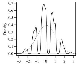
(a) Densities along the optimal direction found using the $m$-spacing method

(b) Densities along the optimal direction found using the fastICA method

Fig. 2: Plots showing an estimate of the density of the projected data (solid line), and the surrogate density $f_{0}$ used in the fastICA method (dotted line), for two different projections of the data. Panel 2(a) corresponds to the direction of highest entropy, found using $m$-spacing, and Panel 2(b) corresponds to the direction found by fastICA. These two directions are shown by the solid line and dotted line respectively in Figure 1.

This paper is structured as follows. In Section 2, entropy and negentropy are introduced alongside associated estimates. In Section 3 we describe the fastICA method. Section 4 contains some proofs which help to understand where errors are introduced in the fastICA method. Section 5 contains details on the example given in Figure 1. Some concluding remarks can be found in Section 6. The code to produce the figures in this paper can be found at https://github.com/pws3141/fastICA_code.

2 Entropy and Negentropy

The aim of the fastICA method is to efficiently find a projection of given data which minimises entropy. Suppose we have a one-dimensional random variable $X$ with density $f\colon\mathbb{R}\rightarrow[0,\infty)$. Then the entropy $H$ of the distribution of $X$ is defined to be

$$H[f]:=-\int_{\mathbb{R}}f(x)\log f(x)\,\text{d}x,$$ (1)

whenever this integral exists. We use square brackets to indicate that $H$ is a functional, taking the function $f$ as its argument. In the special case of a Gaussian random variable with variance $\sigma^{2}$, the entropy can be calculated explicitly and it takes the value $\eta(\sigma^{2})$ given by

$$\eta(\sigma^{2}):=\frac{1}{2}\bigl{(}1+\log(2\pi\sigma^{2})\bigr{)}.$$ (2)

It is known that this is an upper bound for entropy, namely the entropy of any random variable with variance $\sigma^{2}$ will belong to the interval $(-\infty,\eta(\sigma^{2})]$ (see, for example, Cover and Thomas, 2012). The negentropy $J$ is defined as

$$J[f] :=\eta(\sigma^{2})-H[f],$$

where $\eta(\sigma^{2})$ is given by (2). This implies that $J[f]\in[0,\infty)$. Negentropy is zero when the density is Gaussian, and strictly greater than zero otherwise.

As the definition of entropy involves the integral of the density, the estimation of entropy or negentropy from data is non-trivial. For a survey of different methods to estimate entropy from data, see Beirlant et al. (1997). As an example, we consider here the $m$-spacing estimator, originally given in Vasicek (1976). Suppose we have a sample of one-dimensional points, $y_{1},y_{2},\ldots,y_{n}\in\mathbb{R}$, from a distribution with density $f$, and $y_{(1)},y_{(2)},\ldots,y_{(n)}$ is the ordering such that $y_{(1)}\leq y_{(2)}\leq\cdots\leq y_{(n)}$. Define the $m$-spacing difference to be $\Delta_{m}y_{i}=y_{(i+m)}-y_{(i)}$ for $m\in\{3,\ldots,n-1\}$ and $i\in\{1,2,\ldots,n-m\}$. The $m$-spacing approximation for entropy $H[f]$ for the sample $y=(y_{1},y_{2},\ldots,y_{n})$ is given by

$$H_{m,n}(y)=\frac{1}{n}\sum_{i=1}^{n-m}\log\Bigl{(}\frac{n}{m}\,\Delta_{m}y_{i}\Bigr{)}-\digamma(m)+\log(m),$$ (3)

where $\digamma(x)=-\frac{\,\text{d}}{\,\text{d}x}\Gamma(x)$ is the digamma function. This is a realisation of the general $m$-spacing formula given in Hall (1984). This approximation tends to the true value of entropy under certain conditions and so for a “large enough” number of points should be comparable to the true value. This method has been used previously within an ICA method by Learned-Miller and Fisher III (2003). While the methods provides consistent estimates for the entropy, it is computationally expensive. The main contribution to computational cost comes from the need to sort the sample $y$ in increasing order.

The fastICA method provides a more efficient way to estimate negentropy $J[f]$ by using a series of approximations and substitutions both for $f$ and for $J[\cdot]$ to obtain a surrogate for negentropy $J[f]$ which is then subsequently maximised. The reason behind these substitutions is to reduce computational cost, but the drawback is that the resulting approximation may be very different from the true contrast function.

3 The fastICA Algorithm

In this section we describe the fastICA method of Hyvärinen and Oja (2000). The theory behind this method was originally introduced in Hyvärinen (1998), although here we adjust the notation to match the rest of this paper. We will mention explicitly where our notation differs from Hyvärinen (1998) and Hyvärinen and Oja (2000). We will write ‘fastICA’ when we are discussing the theoretical method, and ‘fastICA’ when we are discussing the R implementation from the fastICA CRAN package (Marchini et al., 2013).

The fastICA method to obtain the first loading from data $\tilde{D}\in\mathbb{R}^{n\times\tilde{p}}$ follows the steps given below. Following the usual convention, the rows of $\tilde{D}$ denote observations, the columns denote variables.

1. Whiten the data to obtain $D\in\mathbb{R}^{n\times p}$ with $p=\min(\tilde{p},n-1)$, such that $\frac{1}{n-1}D^{\top}D=I_{p}$ (Hyvärinen and Oja, 2000, Section 5.2);

2. Iteratively find the optimal projection $w^{\ast}$, given by

   $$w^{\ast}=\operatorname*{argmax}_{w\in\mathbb{R}^{p},\,w^{\top}w=1}\hat{J}^{\ast}(Dw),$$ (4)

   where $\hat{J}^{\ast}$ is an approximation to negentropy, given in equation (11) below.

If more than one loading is required, Step ii. is repeated for each subsequent new direction, with the added constraint that $w$ must be orthogonal to the previously found directions. This can be implemented within the fastICA framework using Gram-Schmidt orthogonalisation (Hyvärinen and Oja, 2000, Section 6.2). This is known as the deflation fastICA method. There is also a parallel fastICA method that finds all loadings concurrently, although in this paper we only consider the deflation approach.

In the literature regarding fastICA it is often the convergence of the iterative method to solve (4) that is examined. It can be shown, for example in Wei (2014), that in certain situations this iterative step fails to find a good approximation for $w^{\ast}$. In contrast, here we consider the mathematical substitutions and approximations used in the derivation of $\hat{J}^{\ast}(Dw)$. Assumption 3.1 introduces the technical assumptions given in Hyvärinen (1998, Sections 4 and 6), using slightly adjusted notation.

Assumption 3.1.

Let $G_{i}$, $i=1,2,\ldots,I$ be functions that do not grow faster than quadratically. Let $\varphi(\cdot)$ denote the density of a standard Gaussian random variable and assume that there are $\alpha_{i},\beta_{i},\gamma_{i},\delta_{i}$, $i=1,2,\ldots,I$, such that the functions

$$K_{i}(x):=\frac{G_{i}(x)+\alpha_{i}x^{2}+\beta_{i}x+\gamma_{i}}{\delta_{i}}$$ (5)

satisfy

$$\int_{\mathbb{R}}K_{i}(x)K_{j}(x)\varphi(x)\,\text{d}x =\mathbbm{1}_{\{i=j\}};\text{ and, }$$ (6a)

$$\int_{\mathbb{R}}K_{i}(x)x^{k}\varphi(x)\,\text{d}x =0,\text{ for }k=0,1,2,$$ (6b)

for $i,\,j=1,2,\ldots,I$, where $\mathbbm{1}_{\{i=j\}}=1$ if $i=j$ and zero otherwise.

The functions $G_{i}$ are given as $\bar{G}_{i}$ in Hyvärinen (1998) and as $G_{i}$ in Hyvärinen and Oja (2000). The functions $K_{i}$ are described in Hyvärinen (1998, Section 6) and are called $G_{i}$ there.

The fastICA algorithm only implements the case $I=1$. In this case, the function $G_{1}$ can be chosen nearly arbitrarily so long as it does not grow faster than quadratically: It is easy to show that for every $G$ which is not exactly equal to a second order polynomial, a function $K_{1}$ can be found that satisfies the conditions given in (6) by choosing suitable $\alpha_{1}$, $\beta_{1}$, $\gamma_{1}$ and $\delta_{1}$. For general $I\in\mathbb{N}$, specific $G_{i}$, $i=1,2,\ldots,I$ must be chosen for the conditions (6) to hold. With $I=2$, the functions $G_{1}(x)=x^{3}$ and $G_{2}(x)=x^{4}$ are proposed in the literature (Hyvärinen, 1998, Section $7$) and seem to be useful in practice, even though these functions violate the growth condition from Assumption 3.1. We have not found any examples of specific functions $G_{i}$ that satisfy (6) for $I>2$ in the fastICA literature.

Let $w\in\mathbb{R}^{p}$ with $\|w\|=1$ and let $y=(y_{1},y_{2},\ldots,y_{n})=Dw\in\mathbb{R}^{n}$ be the data projected onto $w$. Since the data has been whitened, $y$ has sample mean $0$ and sample variance $1$. Further, let $f\colon\mathbb{R}\to\mathbb{R}$ be the unknown density of the population-level-whitened and projected data. Then $f$ satisfies $\int f(x)\,dx=1$, $\int x\,f(x)\,dx=0$ and $\int x^{2}\,f(x)\,dx=1$. We need to estimate the negentropy $J[f]$ using the data $y_{1},\ldots,y_{n}$. Define

$$c_{i}:=\mathsf{E}_{f}K_{i}(X)=\int f(x)K_{i}(x)\,\text{d}x$$ (7)

for all $i\in\{1,\ldots I\}$. For $I=1$, setting $K(x):=K_{1}(x)$, $G(x):=G_{1}(x)$ and $c:=c_{1}$, the derivation of the contrast function used in the fastICA method then consists of the following steps:

1. Replace $f$ by a density $f_{0}$ given by

   $$f_{0}(x)=A\exp\Bigl{(}\kappa x+\zeta x^{2}+aK(x)\Bigr{)},$$ (8)

   for all $x\in\mathbb{R}$. The constants $A$, $\kappa$, $\zeta$ and $a$ are chosen to minimise negentropy (and hence maximise entropy) under the constraints $\int f_{0}(x)K(x)\,\text{d}x=c$. In Proposition 4.2 we will show that $J[f_{0}]\leq J[f]$.

2. Approximate $f_{0}$ by $\hat{f}_{0}$ defined as

   $$\hat{f}_{0}(x)=\varphi(x)\bigl{(}1+cK(x)\bigr{)}$$ (9)

   for all $x\in\mathbb{R}$. In Theorem 4.7 we will show $J[\hat{f}_{0}]\approx J[f_{0}]$.

3. Approximate $J[\hat{f}_{0}]$ by second order Taylor expansion,

   $$\hat{J}[\hat{f}_{0}]=\frac{1}{C}\bigl{(}\mathsf{E}_{f}G(Y)-\mathsf{E}_{\varphi}G(Z)\bigr{)}^{2},$$ (10)

   where $Y$ is a random variable with density $f$, $Z\sim\mathcal{N}(0,1)$, and $C$ some constant. Note that, maybe surprisingly, $Y$ has density $f$, not $f_{0}$. In Proposition 4.10 we will show that $\hat{J}[\hat{f}_{0}]\approx J[\hat{f}_{0}]$.

4. Use Monte-Carlo approximation for the expectations in (10), i.e. use

   $$\hat{J}^{\ast}(y)=\Bigl{(}\frac{1}{n}\sum_{j=1}^{n}G(y_{j})-\frac{1}{L}\sum_{j=1}^{L}G(z_{j})\Bigr{)}^{2},$$ (11)

   where $z_{1},\ldots,z_{L}$ are samples from a standard Gaussian and $L$ is large. Here $\hat{J}^{\ast}(y)\approx C\hat{J}[\hat{f}_{0}]$.

The restriction to $I=1$ here removes a summation from Step 1. and Step 2.  therefore simplifying Step 3. and the associated estimations in Step 4. Theoretically these steps can be completed for arbitrary $I\in\mathbb{N}$, although in this case a closed-form version equivalent to Step 3. is much more complicated.

The approximation (11) to the negentropy used in fastICA dramatically decreases the computational time needed to find ICA projections. Unlike the $m$-spacing estimator introduced in Section 2, the approximation $\hat{J}^{\ast}(Dw)$ is a simple Monte-Carlo estimator and does not require sorting of the data. The algorithm to solve (4) also benefits from the fact that an approximate derivative of $w\mapsto\hat{J}^{\ast}(Dw)$ can be derived analytically.

The steps in this chain of approximations are illustrated in Figure 3 and we will investigate the approximation more formally in Section 4. In Step 1. of the procedure, we do not obtain a proper approximation, but have an inequality instead: $f$ is replaced with a density $f_{0}$ such that $J[f_{0}]\leq J[f]$. As a result, the $w$ which maximises $J[f_{0}]$ can be very different from the one which maximises $J[f]$. In contrast, Steps 2. and 3. are proper approximations and in Section 4 we prove convergence of $\hat{f}_{0}$ to $f_{0}$ for Step 2. and of $\hat{J}[\hat{f}_{0}]$ to $J[f_{0}]$ for Step 3. in the limit $\|c\|\to 0$, where $c=(c_{1},\ldots,c_{I})$. Step 4. is a simple Monte-Carlo approximation exhibiting well-understood behaviour. From the above discussion, it seems sensible to surmise that the loss of accuracy in fastICA is due to the surrogate used in Step 1. above.

Fig. 3: Approximations used in fastICA: The fastICA contrast function $\hat{J}^{\ast}(y)$ is used in place of negentropy $J[f]$. Note that the first step involves an inequality rather than an approximation.

We conclude this section with a few simple observations: Using (6), (5) and the fact that $X$ and $Z$ are standardized we find

$$c_{i} =\mathsf{E}_{f}K_{i}(X)$$

$$=\mathsf{E}_{f}K_{i}(X)-\mathsf{E}_{\varphi}K_{i}(Z)$$

$$=\mathsf{E}_{f}\left(\frac{G_{i}(X)+\alpha_{i}X^{2}+\beta_{i}X+\gamma_{i}}{\delta_{i}}\right)-\mathsf{E}_{\varphi}\left(\frac{G_{i}(Z)+\alpha_{i}Z^{2}+\beta_{i}Z+\gamma_{i}}{\delta_{i}}\right)$$

$$=\frac{\mathsf{E}_{f}G_{i}(X)+\alpha_{i}1+\beta_{i}0+\gamma_{i}}{\delta_{i}}-\frac{\mathsf{E}_{\varphi}G_{i}(Z)+\alpha_{i}1+\beta_{i}0+\gamma_{i}}{\delta_{i}}$$

$$=\frac{\mathsf{E}_{f}G_{i}(X)-\mathsf{E}_{\varphi}G_{i}(Z)}{\delta_{i}}.$$

Thus, the fastICA objective function (ignoring the final Monte Carlo approximation) satisfies $\hat{J}[\hat{f}_{0}]\propto c^{2}$ for the case $I=1$, considered above, and $\hat{J}[\hat{f}_{0}]\propto\sum_{i=1}^{I}c_{i}^{2}$ in the general case. Thus, fastICA can only see the data through the $c_{i}$. If the data are approximately Gaussian, we have $\mathsf{E}_{f}G_{i}(X)\approx\mathsf{E}_{\varphi}G_{i}(Z)$ and $c_{i}\approx 0$ for all $i$ and thus $\hat{J}[\hat{f}_{0}]\approx 0$, but the opposite implication does not hold. This is in contrast to the true negentropy, which satisfies $J[f]=0$ if and only if $f$ is Gaussian.

A first consequence of this argument is that projections where the true distribution is Gaussian will look ‘uninteresting’ to fastICA: for these directions $w$ the objective function $\hat{J}^{\ast}(Dw)$ will be small and the search for the maximum in (4) will be driven away from these directions. This is particularly relevant since for high dimensional data, where the search volume is vast, projections along most directions are close to Gaussian (Diaconis and Freedman, 1984; von Weizsäcker, 1997), so fastICA will be able to exclude much of the search volume. Conversely, if $\hat{J}[\hat{f}_{0}]$ and thus $\|c\|$ is large, the projected density $f$ is not Gaussian and by maximising (an approximation to) $\hat{J}[\hat{f}_{0}]$, the fastICA method will find directions which are ‘interesting’. But the above discussion also shows that optima can be missed when $\hat{J}[\hat{f}_{0}]$ is small, but the projected density $f$ is still far from Gaussian. This is the case we are concerned with in this paper and thus we assume $\|c\|\approx 0$ when we consider the fastICA approximations in detail in the next section.

4 Approximations used in the fastICA Method

In this section, we investigate the validity of the approximation given in Section 3. We consider Step 1. in Proposition 4.2, Step 2. in Theorem 4.7, and Step 3. in Proposition 4.10. Throughout this section, we consider arbitrary $I\in\mathbb{N}$ for completeness.

We first introduce some assumptions, in addition to Assumption 3.1, that are required for the mathematics in this section to hold.

Assumption 4.1.

There exists $\varepsilon>0$ such that for all $h\in\mathbb{R}^{I}$ with $h^{\top}h<\varepsilon$, we have

$$h^{\top}K(x)\geq-\frac{1}{2}$$ (12)

for all $x\in\mathbb{R}$, where $K(x)=\bigl{(}K_{1}(x),K_{2}(x),\ldots,K_{I}(x)\bigr{)}$. In addition, there exists a function $M\colon\mathbb{R}\rightarrow\mathbb{R}$ such that

$$\sum_{i=1}^{I}\sum_{j=1}^{I}\sum_{k=1}^{I}\lvert K_{i}(x)K_{j}(x)K_{k}(x)\rvert \leq M(x)\text{ for all }x\in\mathbb{R},\text{ and}$$ (13a)

$$\int_{\mathbb{R}}\varphi(x)M(x)\,\text{d}x =:\tilde{M}<\infty.$$ (13b)

Note that under the condition that each $G_{i}$ does not grow faster than quadratically (given in Assumption 3.1), we can always find some positive constants $B_{i}$, $i=1,2,\ldots,I$ such that

$$\lvert K_{i}(x)\rvert\leq B_{i}(1+x^{2}),$$ (14)

for all $x\in\mathbb{R}$. Note also that for $I=1$ the condition given by (12) that there exists an $\varepsilon>0$ such that for all $h\in[0,\varepsilon)$, we have $hK(x)\geq-1/2$ is satisfied as follows. Let $\alpha,\beta,\gamma,\delta$ be parameters for which (6) holds. Then, (6) holds also for $\alpha,\beta,\gamma,-\delta$. Moreover, since $G$ does not grow faster than quadratically, $\alpha x^{2}$ is the dominant term in $K(x)$ as $x\rightarrow\pm\infty$. Therefore, to ensure that (12) holds it is enough to choose $\delta$ or $-\delta$ such that the sign is the same as that of $\alpha$.

4.1 Step 1.

We start our discussion by considering Step 1. of the approximations described in Section 3. We prove that the distribution which maximises entropy for given values of $c_{1},\ldots,c_{I}$ is indeed of the form (8) and thus that we indeed have $J[f_{0}]\leq J[f]$.

Proposition 4.2.

Let $f$ be the density of the population-level-whitened data projected in some direction (thus with zero mean and unit variance). Recall $c_{i}$ is defined by (7). The density $f_{0}$ that maximises entropy in the set

$$\Bigl{\{}g\colon\mathbb{R}\rightarrow\mathbb{R}\,;\,g\text{ is a density function, and }\int_{\mathbb{R}}g(x)K_{i}(x)\,\text{d}x=c_{i},\,i=1,2,\ldots,I\Bigr{\}},$$

is given by,

$$f_{0}(x)=A\exp\left(\kappa x+\zeta x^{2}+\sum_{i=1}^{I}a_{i}K_{i}(x)\right)$$ (15)

for some constants $\kappa$, $\zeta$, $A$ and $a_{i},\,i=1,2,\ldots,I$ that depend on $c_{i},\,i=1,2,\ldots,I$. It follows from this that $J[f_{0}]\leq J[f]$.

Proof.

We use the method of Lagrange multipliers in the calculus of variations (see, for example, Lawrence, 1998) to find a necessary condition for the density that maximises entropy given the constraints on mean and variance, and in (7). Let $F[\cdot]\colon C^{2}\rightarrow\mathbb{R}$ be a functional of the function $g\colon\mathbb{R}\rightarrow\mathbb{R}$, with $g\in C^{2}$, where $C^{2}$ is the set of all twice continuously differentiable functions. Then, the functional derivative $\delta F/\delta g\colon\mathbb{R}\rightarrow\mathbb{R}$ is explicitly defined by

$$\int_{\mathbb{R}}\frac{\delta F}{\delta g}(x)\phi(x)\,\text{d}x:=\frac{\,\text{d}}{\,\text{d}\varepsilon}F[g+\varepsilon\phi]\Bigr{|}_{\varepsilon=0}=\lim_{\varepsilon\downarrow 0}\Bigl{(}\frac{F[g+\varepsilon\phi]-F[g]}{\varepsilon}\Bigr{)},$$ (16)

for any function $\phi\in C^{2}$. The right-hand side of (16) is known as the Gâteaux differential $\,\text{d}F(g;\phi)$. Define the inner product of two functions by $\langle g,h\rangle:=\int_{\mathbb{R}}g(x)h(x)\,\text{d}x$, with norm $\lVert g\rVert_{\text{L}^{2}}:=\langle g,g\rangle^{\frac{1}{2}}=\bigl{(}\int_{\mathbb{R}}g(x)^{2}\,\text{d}x\bigr{)}^{\frac{1}{2}}$. We want to solve the following system of equations

$$\begin{cases}U[g](x)&:=\frac{\delta}{\delta g}H[g]+\lambda_{1}\frac{\delta}{\delta g}V[g]+\lambda_{2}\frac{\delta}{\delta g}P[g]+\lambda_{3}\frac{\delta}{\delta g}Q[g]+\sum_{i=1}^{I}\nu_{i}\frac{\delta}{\delta g}R_{i}[g]=0;\\ V[g]&=0;\\ P[g]&=0;\\ Q[g]&=0;\\ R_{i}[g]&=0,\end{cases}$$

where $\lambda_{1},\lambda_{2},\lambda_{3},\nu_{i},i=1,\ldots,I$ are some real numbers, $H[g]$ is entropy as given in (1), and

$$V[g] :=\mathrm{Var}[g]-1=\int_{\mathbb{R}}g(x)x^{2}\,\text{d}x-\Bigl{(}\int_{\mathbb{R}}g(x)x\,\text{d}x\Bigr{)}^{2}-1;$$

$$P[g] :=\int_{\mathbb{R}}g(x)\,\text{d}x-1;$$

$$Q[g] :=\int_{\mathbb{R}}g(x)x\,\text{d}x;$$

$$R_{i}[g] :=\int_{\mathbb{R}}g(x)K_{i}(x)\,\text{d}x-c_{i}.$$

Using (1) and (16) the term with $H$ gives,

$$\langle\frac{\delta H}{\delta g},\phi\rangle =-\frac{\,\text{d}}{\,\text{d}\varepsilon}\int\bigl{(}g(x)+\varepsilon\phi(x)\bigr{)}\log\bigl{(}g(x)+\varepsilon\phi(x)\bigr{)}\,\text{d}x\Bigr{|}_{\varepsilon=0}$$

$$=-\int\Bigl{(}g(x)\frac{\phi(x)}{g(x)+\varepsilon\phi(x)}+\phi(x)\log\bigl{(}g(x)+\varepsilon\phi(x)\bigr{)}+\varepsilon\phi(x)\frac{\phi(x)}{g(x)+\varepsilon\phi(x)}\Bigr{)}\,\text{d}x\Bigr{|}_{\varepsilon=0}$$

$$=-\int\bigl{(}1+\log g(x)\bigr{)}\phi(x)\,\text{d}x$$

$$=\langle-1-\log g(x),\phi\rangle.$$

Now, looking at $V[g]$ and using the constraint $Q[g]=0$ we get,

$$\langle\frac{\delta V}{\delta g},\phi\rangle =\frac{\,\text{d}}{\,\text{d}\varepsilon}\biggl{(}\int\bigl{(}g(x)+\varepsilon\phi(x)\bigr{)}x^{2}\,\text{d}x-\Bigl{(}\int\bigl{(}g(x)+\varepsilon\phi(x)\bigr{)}x\,\text{d}x\Bigr{)}^{2}-1\biggr{)}\biggr{|}_{\varepsilon=0}$$

$$=\int\phi(x)x^{2}\,\text{d}x-2\Bigl{(}\int\phi(x)x\,\text{d}x\cdot\int g(x)x\,\text{d}x\Bigr{)}$$

$$=\langle x^{2},\phi\rangle-2\langle x,\phi\rangle\cdot Q[g]$$

$$=\langle x^{2},\phi\rangle.$$

Let $L[\cdot]\colon C^{2}\rightarrow\mathbb{R}$ be of the form $L[g]=\int g(x)l(x)\,\text{d}x-k$ for some function $l\colon\mathbb{R}\rightarrow\mathbb{R}$, and some constant $k\in\mathbb{R}$. Then it is easy to check that $\langle\dfrac{\delta L}{\delta g},\phi\rangle=\langle l,\phi\rangle$ and therefore $\dfrac{\delta P}{\delta g}=1$, $\dfrac{\delta Q}{\delta g}=x$ and $\dfrac{\delta R_{i}}{\delta g}=K_{i}$. Putting this into the equation for $U[g]$, we have

$$U[g](x)=-1-\log g(x)+\lambda_{1}+\lambda_{2}x^{2}+\lambda_{3}x+\sum_{i=1}^{I}\nu_{i}K_{i}(x).$$

Setting $U[g]=0$ and solving for $g$ gives, $g(x)=f_{0}(x)=\exp[\lambda_{1}-1+\lambda_{2}x^{2}+\lambda_{3}x+\sum_{i=1}^{I}\nu_{i}K_{i}(x)]$ which is (15) with $A=\exp(\lambda_{1}-1)$, $\kappa=\lambda_{3}$, $\zeta=\lambda_{2}$ and $a_{i}=\nu_{i}$, $i=1,\ldots,I$. Note that the constants $A,\,\kappa,\,\zeta$, and $a_{i}$ depend on $c_{i}$ indirectly through the constraints on the $K_{i}$ expressed as $R_{i}[g]=0$. ∎

Remark 4.3.

It is possible to specify a density $f$ such that in some limit, $H[f]\rightarrow\infty$ whilst $H[f_{0}]$ remains bounded and thus $\bigl{|}J[f]-J[f_{0}]\bigr{|}\rightarrow\infty$, with $f_{0}$ the density given in (8). That is, in Step 1. of the fastICA method given in Section 3, the difference between the true negentropy and the surrogate negentropy can be arbitrarily large. For example, set the density $f$ to be a mixture of two independent uniform densities, i.e.

$$f(x)=\frac{1}{2}\bigl{(}g(x;\,-1-\varepsilon,-1)+g(x;\,1,1+\varepsilon)\bigr{)}$$

where $\varepsilon\in\mathbb{R}$ and $g(\cdot\,;\,a,b)$ is the density function of a Uniform distribution in the interval $[a,b]$. Then we have expectation and variance given by

$$\mathsf{E}_{f}X=0;\quad\mathrm{Var}_{f}X=1+\varepsilon+\frac{\varepsilon^{2}}{3}.$$

As the support of $g(\cdot\,;\,-1-\varepsilon,-1)$ is disjoint from that of $g(\cdot\,;\,1,1+\varepsilon)$, the entropy is given by,

$$H[f]=\frac{1}{2}\bigl{(}H[g(\cdot\,;\,-1-\varepsilon,-1)]+H[g(\cdot\,;\,1,1+\varepsilon)]\bigr{)}-\log(2).$$

We have $H[f]\rightarrow-\infty$ as $\varepsilon\rightarrow 0$, since $f$ tends to a pair of Dirac deltas. Also,

$$\mathsf{E}_{f}K_{i}(x)=:c_{i}\rightarrow\frac{1}{2}\bigl{(}K_{i}(-1)+K_{i}(1)\bigr{)},$$ (17)

as $\varepsilon\rightarrow 0$. With $f_{0}$ as in (8),

$$c_{i}=\int K_{i}(x)f_{0}(x)\,\text{d}x,$$ (18)

and,

$$H[f_{0}] =\int f_{0}(x)\log(A)\,\text{d}x+\int f_{0}(x)\bigl{(}\eta x+\kappa x^{2}+\sum_{i=1}^{I}a_{i}K_{i}(x)\bigr{)}\,\text{d}x$$

$$=\log(A)+\eta\mathsf{E}_{f_{0}}X+\kappa\mathsf{E}_{f_{0}}X^{2}+\sum_{i=1}^{I}a_{i}\mathsf{E}_{f_{0}}K_{i}(x)$$

$$=\log(A)+\kappa+\sum_{i=1}^{I}a_{i}c_{i}.$$

Therefore, for $H[f_{0}]$ to be unbounded from below as $\varepsilon\rightarrow 0$ we would require some $\kappa\rightarrow-\infty$, $a_{i}\rightarrow-\infty$ or $A\rightarrow 0$, as $c_{i}$ is bounded by (17) and Assumption 4.1. However, this can not occur whilst $f_{0}$ satisfies (18).

4.2 Step 2.

We now switch our attention to Step 2. of the approximations. As discussed in Section 3, we consider the case where $c\rightarrow 0$. The first step of our analysis is to identify the behaviour of the constants in the definition of $f_{0}$ as $c\to 0$. We then prove some auxiliary results before concluding our discussion of Step 2. in Theorem 4.7.

Proposition 4.4.

Suppose Assumption 3.1 is satisfied, and let $A,\kappa,\zeta,a_{1},\dots,a_{I}$ be defined as in Proposition 4.2, as functions of $c$. Then

$$\begin{split}A-\frac{1}{\sqrt{2\pi}}&=\mathcal{O}(\lVert c\rVert^{2})\\ \kappa&=\mathcal{O}(\lVert c\rVert^{2})\\ \zeta+\frac{1}{2}&=\mathcal{O}(\lVert c\rVert^{2})\\ a_{i}-c_{i}&=\mathcal{O}(\lVert c\rVert^{2}),\quad i=1,2,\ldots,I,\end{split}$$

as $\|c\|\rightarrow 0$.

Proof.

Define $x=(c_{1},\ldots,c_{I})^{\top}\in\mathbb{R}^{I}$ and $y=(A,\kappa,\zeta,a_{1},\ldots,a_{I})^{\top}\in\mathbb{R}^{I+3}$. Furthermore, let $F\colon\mathbb{R}^{I}\times\mathbb{R}^{I+3}\rightarrow\mathbb{R}^{I+3}$ be given by

$$F(x,y)=\begin{pmatrix}\int f_{0}(x)\,\text{d}x-1\\ \int f_{0}(x)x\,\text{d}x\\ \int f_{0}(x)x^{2}\,\text{d}x-1\\ \int f_{0}(x)K_{1}(x)\,\text{d}x-c_{1}\\ \vdots\\ \int f_{0}(x)K_{I}(x)\,\text{d}x-c_{I}\end{pmatrix},$$

where $f_{0}$ is given in (15) and $K_{i}$ in (5). Then, for the points $x_{1}=(0,\ldots,0)^{\top}$ and $y_{1}=(\tfrac{1}{\sqrt{2\pi}},0,-\tfrac{1}{2},0,\ldots,0)^{\top}$, we have $F(x_{1},y_{1})=0$.

Assuming $F$ is twice differentiable, we use the Implicit Function Theorem (see, for example, de Oliveira, 2014) around $(x_{1},y_{1})$. First, we need to show $D_{y}F(x_{1},y_{1})$ is invertible. We have

$$D_{y}F(x_{1},y_{1})=\begin{pmatrix}M&0\\ 0&-I_{I}\end{pmatrix},\quad\text{with, }M=\begin{pmatrix}\sqrt{2}&0&1\\ 0&1&0\\ 1&0&4\end{pmatrix}.$$

Therefore, $D_{y}F(x_{1},y_{1})$ is non-singular, and so the Implicit Function Theorem holds. There exist some open set $\mathcal{U}\subset\mathbb{R}^{I}$ and a unique continuously differentiable function $g\colon\mathcal{U}\rightarrow\mathbb{R}^{I+3}$ such that $g(x_{1})=y_{1}$ and $F\bigl{(}x,\,g(x)\bigr{)}=0$ for all $x\in\mathcal{U}$. Then,

$$Dg(x)=-D_{y}F\bigl{(}x,\,g(x)\bigr{)}^{-1}D_{x}F\bigl{(}x,\,g(x)\bigr{)}.$$ (19)

As $g$ is continuous in the set $\mathcal{U}$, there exists some $\varepsilon>0$, such that for all $c\in\mathcal{U}$ with $\lVert c\rVert<\varepsilon$, $g(x_{1}+c)=y_{1}+d$ for some $d\in\mathbb{R}^{I+3}$. Using Taylor series we can expand $g$ around $x_{1}=0\in\mathbb{R}^{I}$ to obtain $g(x_{1}+c)=g(x_{1})+Dg(x_{1})\,c+\mathcal{O}(\lVert c\rVert^{2})$, and

$$Dg(x_{1})=\frac{d+\mathcal{O}(\lVert c\rVert^{2})}{c}.$$

Putting this together with (19) at $x=x_{1}$ and rearranging gives,

$$d=-D_{y}F(x_{1},y_{1})^{-1}D_{x}F(x_{1},y_{1})\,c+\mathcal{O}(\lVert c\rVert^{2}).$$

Now, since

$$D_{x}F(x_{1},y_{1})=\begin{pmatrix}0&\cdots&0\\ 0&\cdots&0\\ 0&\cdots&0\\ &I_{I}&\end{pmatrix}\in\mathbb{R}^{(I+3)\times I},$$

one easily obtains that

$$d=\begin{pmatrix}0&\cdots&0\\ 0&\cdots&0\\ 0&\cdots&0\\ &I_{I}&\end{pmatrix}c+\mathcal{O}(\lVert c\rVert^{2}),$$

and so,

$$y_{1}+d=\begin{pmatrix}\frac{1}{\sqrt{2\pi}}\\ 0\\ -\frac{1}{2}\\ c_{1}\\ \vdots\\ c_{I}\end{pmatrix}+\mathcal{O}(\lVert c\rVert^{2}),\text{ as }c\rightarrow 0.$$

This completes the proof. ∎

We now define the following functions $y(\cdot)$ and $r(\cdot)$ for future use. Let $y\colon\mathbb{R}\rightarrow\mathbb{R}$ be given by

$$y(x):=\kappa x+(\zeta+\frac{1}{2})x^{2}+\sum_{i=1}^{I}a_{i}K_{i}(x),$$ (20)

and $r\colon\mathbb{R}\rightarrow\mathbb{R}$ given by

$$r(x):=e^{x}-1-x.$$ (21)

Using these definitions, we can write $f_{0}$, given in Proposition 4.2, as

$$f_{0}(x)=\varphi(x)\cdot\sqrt{2\pi}Ae^{y(x)}.$$ (22)

The following lemmas are two technical results needed in the proof of Theorem  4.7.

Lemma 4.5.

Let $g\colon\mathbb{R}\rightarrow\mathbb{R}$ and $l\colon\mathbb{R}\rightarrow\mathbb{R}$ be any functions and $h\colon\mathbb{R}\rightarrow\mathbb{R}_{+}$ be convex with $h(0)=0$. Then,

$$\sup_{x\in\mathbb{R}}\bigl{\lvert}l(x)h(\varepsilon g(x))\bigr{\rvert}\leq\varepsilon\,\sup_{x\in\mathbb{R}}\bigl{\lvert}l(x)h(g(x))\bigr{\rvert}$$

for all $\varepsilon\in[0,1]$.

Proof.

As $h$ is convex, for all $\lambda\in[0,1]$ and for all $x,y\in\mathbb{R}$, we have $h\bigl{(}\lambda x+(1-\lambda)y\bigr{)}\leq\lambda h(x)+(1-\lambda)h(y)$. Let $\varepsilon\in[0,1]$. Then, substituting $\lambda=\varepsilon$, $x=g(x)$ and $y=0$, we have $h\bigl{(}\varepsilon\,g(x)\bigr{)}\leq\varepsilon\,h\bigl{(}g(x)\bigr{)}$, for all $g(x)\in\mathbb{R}$, as $h(0)=0$. Noticing that $h$ maps to the positive real line allows to conclude. ∎

Lemma 4.6.

Let $r\colon\mathbb{R}\rightarrow\mathbb{R}_{+}$ be given as in (21). Then,

$$r(\varepsilon\,y)\leq\varepsilon^{2}r(y),\text{ for all $y\geq 0$, and for all $\varepsilon\in[0,1]$.}$$ (23)

Moreover, for any function $l\colon\mathbb{R}\rightarrow\mathbb{R}$, we have

$$\sup_{x\in\mathbb{R}}\Bigl{\lvert}l(x)r\bigl{(}\varepsilon(1+x^{2})\bigr{)}\Bigr{\rvert}\leq\varepsilon^{2}\sup_{x\in\mathbb{R}}\Bigl{\lvert}l(x)r(1+x^{2})\Bigr{\rvert}.$$

Proof.

We will use the Taylor expansion of the exponential around $0$ for both the left-hand and right-hand side of (23). The left-hand side gives,

$$r(\varepsilon\,y) =\exp(\varepsilon\,y)-1-\varepsilon\,y$$

$$=\sum_{n=0}^{\infty}\frac{\varepsilon^{n}}{n!}\,y^{n}-1-\varepsilon\,y,\quad\text{absolutely convergent for all }\varepsilon y\in\mathbb{R}$$

$$=\varepsilon^{2}\,\Bigl{(}\sum_{n=2}^{\infty}\frac{\varepsilon^{n-2}}{n!}y^{n}\Bigl{)}$$

and the right-hand side of (23) gives,

$$\varepsilon^{2}\,r(y) =\varepsilon^{2}\,\Bigl{(}\sum_{n=0}^{\infty}\frac{1}{n!}\,y^{n}-1-y\Bigl{)}=\varepsilon^{2}\,\Bigl{(}\sum_{n=2}^{\infty}\frac{1}{n!}\,y^{n}\Bigr{)}.$$

Putting these two results together,

$$r(\varepsilon\,y)-\varepsilon^{2}\,r(y)=\varepsilon^{2}\Bigl{(}\sum_{n=2}^{\infty}\frac{1}{n!}\,y^{n}(\varepsilon^{n-2}-1)\Bigr{)}\leq 0,$$

as $\varepsilon^{n}-1\leq 0$ for all $\varepsilon\in[0,1]$ and $n\in\mathbb{N}_{+}$. This proves (23).

Let $l\colon\mathbb{R}\to\mathbb{R}$ be some function. Then, as $r$ maps to the positive real line and using (23) with $y=1+x^{2}$, we have $\lvert l(x)r\bigl{(}\varepsilon(1+x^{2})\bigr{)}\rvert\leq\varepsilon^{2}\lvert l(x)r(1+x^{2})\rvert$, for all $x\in\mathbb{R}$. Taking the supremum over the real line we conclude. ∎

We now consider the error term between the density $f_{0}$ that maximises entropy, and its estimate $\hat{f}_{0}$.

Theorem 4.7.

Suppose we have functions $K_{i}$, $i=1,2,\ldots,I$ that satisfy Assumptions 3.1 and 4.1. Let $f_{0}$ be given as in Proposition 4.2, and let $\hat{f}_{0}$ be given by

$$\hat{f}_{0}(x)=\varphi(x)\Bigl{(}1+\sum_{i=1}^{I}c_{i}K_{i}(x)\Bigr{)}.$$

Then,

$$\sup_{x\in\mathbb{R}}\bigl{\lvert}e^{\delta x^{2}}\bigl{(}f_{0}(x)-\hat{f}_{0}(x)\bigr{)}\bigr{\rvert}=\mathcal{O}(\lVert c\rVert^{2})\text{ as }c\rightarrow 0,$$

for all $\delta<1/2$.

Proof.

Let $\varphi(x)=(2\pi)^{1/2}e^{-x^{2}/2}$ be the density of a standard Gaussian random variable and let the function $g\colon\mathbb{R}\rightarrow\mathbb{R}$ be defined by

$$g(x):=\frac{f_{0}(x)-\hat{f}_{0}(x)}{\varphi(x)}.$$

Then, with $y\colon\mathbb{R}\rightarrow\mathbb{R}$ as defined in (20) and using (22) we get,

$$g(x) =\sqrt{2\pi}A\exp\bigl{(}y(x)\bigr{)}-\bigl{(}1+\sum_{i=1}^{I}c_{i}K_{i}(x)\bigr{)}$$

$$=\sqrt{2\pi}A\Bigl{(}\exp\bigl{(}y(x)\bigr{)}-1-y(x)\Bigr{)}+\sqrt{2\pi}A\bigl{(}1+y(x)\bigr{)}-(1+\sum_{i=1}^{I}c_{i}K_{i}(x))$$

$$\quad+\sqrt{2\pi}A\bigl{(}\sum_{i=1}^{I}c_{i}K_{i}(x)-\sum_{i=1}^{I}c_{i}K_{i}(x)\bigr{)}.$$

Rearranging this using the function $r\colon\mathbb{R}\rightarrow\mathbb{R}$ given in  (21) and by expanding $y(x)$ gives,

$$g(x) =\sqrt{2\pi}A\cdot r\bigl{(}y(x)\bigr{)}+\sqrt{2\pi}A\cdot\Bigl{(}\kappa x+\bigl{(}\zeta+\frac{1}{2}\bigr{)}x^{2}\Bigr{)}$$

$$\quad+\bigl{(}\sqrt{2\pi}A-1\bigr{)}\sum_{i=1}^{I}c_{i}K_{i}(x)+\sqrt{2\pi}A\sum_{i=1}^{I}(a_{i}-c_{i})K_{i}(x)+(\sqrt{2\pi}A-1).$$

Note that the absolute value of $g(x)$ can be bounded by the following terms,

$$\lvert g(x)\rvert \leq\sqrt{2\pi}A\,\lvert r\bigl{(}y(x)\bigr{)}\rvert+\sqrt{2\pi}A\,\lvert\kappa x\rvert+\sqrt{2\pi}A\,\lvert\zeta+\frac{1}{2}\rvert x^{2}$$

$$\hskip 28.45274pt+\sqrt{2\pi}A\,\bigl{\lvert}\sum_{i=1}^{I}(a_{i}-c_{i})K_{i}(x)\bigr{\rvert}+\lvert\sqrt{2\pi}A-1\rvert\,\bigl{\lvert}\sum_{i=1}^{I}c_{i}K_{i}(x)\bigr{\rvert}+\lvert\sqrt{2\pi}A-1\rvert.$$

We have,

$$\begin{split}\lvert f_{0}(x)-\hat{f}_{0}(x)\rvert&=\lvert\varphi(x)\cdot g(x)\rvert\\ &=\varphi(x)\Bigl{\lvert}\sqrt{2\pi}Ar\bigl{(}y(x)\bigr{)}+\sqrt{2\pi}A\Bigl{(}\kappa x+\bigl{(}\zeta+\frac{1}{2}\bigr{)}x^{2}\Bigr{)}+(\sqrt{2\pi}A-1)\sum_{i=1}^{I}c_{i}K_{i}(x)\Bigr{.}\\ &\hskip 42.67912pt\Bigl{.}+\sqrt{2\pi}A\sum_{i=1}^{I}(a_{i}-c_{i})K_{i}(x)+(\sqrt{2\pi}A-1)\Bigr{\rvert}.\end{split}$$

We now multiply both sides by $e^{\delta x^{2}}$ and setting $\tilde{\delta}=\frac{1}{2}-\delta$, so that $e^{\delta x^{2}}\varphi(x)=(2\pi)^{-1/2}e^{-\tilde{\delta}x^{2}}$, we have

$$\bigl{\lvert}e^{\delta x^{2}}\bigl{(}f_{0}(x)-\hat{f}_{0}(x)\bigr{)}\bigr{\rvert} =(2\pi)^{-1/2}e^{-\tilde{\delta}x^{2}}\Bigl{\lvert}\sqrt{2\pi}Ar\bigl{(}y(x)\bigr{)}+\sqrt{2\pi}A\Bigl{(}\kappa x+\bigl{(}\zeta+\frac{1}{2}\bigr{)}x^{2}\Bigr{)}$$

$$\hskip 79.6678pt\Bigl{.}+(\sqrt{2\pi}A-1)\sum_{i=1}^{I}c_{i}K_{i}(x)+\sqrt{2\pi}A\sum_{i=1}^{I}(a_{i}-c_{i})K_{i}(x)$$

$$\hskip 79.6678pt+(\sqrt{2\pi}A-1)\Bigr{\rvert}$$

$$\leq T_{1}(x)+T_{2}(x)+\frac{1}{\sqrt{2\pi}}\cdot T_{3}(x)+T_{4}(x)+\frac{1}{\sqrt{2\pi}}\cdot T_{5}(x),$$ (24)

where,

$$T_{1}(x) :=\bigl{\lvert}Ae^{-\tilde{\delta}x^{2}}r\bigl{(}y(x)\bigr{)}\bigr{\rvert};$$

$$T_{2}(x) :=\bigl{\lvert}Ae^{-\tilde{\delta}x^{2}}\bigl{(}\kappa x+(\zeta+\frac{1}{2})x^{2}\bigr{)}\bigr{\rvert};$$

$$T_{3}(x) :=\bigl{\lvert}(\sqrt{2\pi}A-1)e^{-\tilde{\delta}x^{2}}\sum_{i=1}^{I}c_{i}K_{i}(x)\bigr{\rvert};$$

$$T_{4}(x) :=\bigl{\lvert}Ae^{-\tilde{\delta}x^{2}}\sum_{i=1}^{I}(a_{i}-c_{i})K_{i}(x)\bigr{\rvert};$$

$$T_{5}(x) :=\lvert e^{-\tilde{\delta}x^{2}}(\sqrt{2\pi}A-1)\rvert.$$

If we show that $\lVert T_{i}\rVert_{\infty}$ is at least of order $\lVert c\rVert^{2}$ as $c\rightarrow 0$ for $i=1,\ldots,5$, then we can conclude the proof by taking the supremum of (24) over $x\in\mathbb{R}$, which gives,

$$\sup_{x\in\mathbb{R}}\bigl{\lvert}e^{\delta x^{2}}(f_{0}(x)-\hat{f}_{0}(x))\bigr{\rvert}=\mathcal{O}(\lVert c\rVert^{2}),$$

as $c\rightarrow 0$.

Term $\bm{T_{1}}$. First, note that

$$\bigl{\lvert}e^{-\tilde{\delta}x^{2}}r(y(x))\bigr{\rvert}\leq\max_{\sigma\in\{-1,1\}}\bigl{\lvert}e^{-\tilde{\delta}x^{2}}r(\sigma\cdot\lvert y(x)\rvert)\bigr{\rvert},\text{ for all }x\in\mathbb{R},$$

and thus,

$$\sup_{x\in\mathbb{R}}\lvert T_{1}(x)\rvert\leq A\cdot\sup_{{\begin{subarray}{c}x\in\mathbb{R}\\ \sigma\in\{-1,1\}\end{subarray}}}\lvert e^{-\tilde{\delta}x^{2}}r(\sigma\cdot\lvert y(x)\rvert)\rvert.$$ (25)

Next we choose $\gamma$ such that,

$$q_{1}:=\sup_{{\begin{subarray}{c}x\in\mathbb{R}\\ \sigma\in\{-1,1\}\end{subarray}}}\bigl{\lvert}e^{-\tilde{\delta}x^{2}}r\bigl{(}\sigma\cdot\gamma(1+x^{2})\bigr{)}\bigr{\rvert}<\infty.$$ (26)

This is always possible for some $\gamma\in(-\tilde{\delta},\tilde{\delta})$, as $r(0)=0$, and since $e^{-\tilde{\delta}x^{2}}r\bigl{(}\pm\gamma(1+x^{2})\bigr{)}$ is continuous and $r\bigl{(}\pm\gamma(1+x^{2})\bigr{)}$ grows no faster that $e^{\gamma x^{2}}$ as $x\rightarrow\pm\infty$, it is beaten by $e^{-\tilde{\delta}x^{2}}$ in the tails.
For $y(x)$ as given in (20) and using  (14) we can find an upper bound by

$$\lvert y(x)\rvert \leq\lvert\kappa\rvert\cdot\Bigl{(}\frac{1+x^{2}}{2}\Bigr{)}+\lvert\zeta+\frac{1}{2}\rvert\cdot(1+x^{2})+\sum_{i=1}^{I}\lvert a_{i}\rvert B_{i}(1+x^{2})$$

$$=\gamma(1+x^{2})\cdot\frac{1}{\gamma}\Bigl{(}\frac{1}{2}\lvert\kappa\rvert+\lvert\zeta+\frac{1}{2}\rvert+\sum_{i=1}^{I}\lvert a_{i}\rvert B_{i}\Bigr{)}$$

$$=:\gamma(1+x^{2})\cdot\varepsilon_{1},$$ (27)

where $\gamma$ is such that (26) holds. As $c\rightarrow 0$, we have by Proposition 4.4, $\kappa\rightarrow 0$, $\zeta\rightarrow-1/2$ and $a_{i}\rightarrow c_{i}$. Therefore, we can choose $c$ small enough (and depending on $\gamma$) such that $\varepsilon_{1}\in[0,1]$. Now, from (25), (27), the fact that $r$ is convex with a minimum at zero, and by Lemma 4.6 we get

$$\sup_{x\in\mathbb{R}}\bigl{\lvert}T_{1}(x)\bigr{\rvert} \leq A\sup_{{\begin{subarray}{c}x\in\mathbb{R}\\ \sigma\in\{-1,1\}\end{subarray}}}\bigl{\lvert}e^{-\tilde{\delta}x^{2}}r\bigl{(}\sigma\gamma(1+x^{2})\varepsilon_{1}\bigr{)}\bigr{\rvert}$$

$$\leq\varepsilon_{1}^{2}A\sup_{{\begin{subarray}{c}x\in\mathbb{R}\\ \sigma\in\{-1,1\}\end{subarray}}}\bigl{\lvert}e^{-\tilde{\delta}x^{2}}r\bigl{(}\sigma\gamma(1+x^{2})\bigr{)}\bigr{\rvert}$$

$$=\varepsilon_{1}^{2}\,A\,q_{1}.$$

By Proposition 4.4, we have $A\rightarrow 1/\sqrt{2\pi}$ as $c\rightarrow 0$ and,

$$\varepsilon_{1}=\frac{1}{\gamma}\Bigl{(}\frac{1}{2}\lvert\kappa\rvert+\lvert\zeta+\frac{1}{2}\rvert+\sum_{i=1}^{I}\lvert a_{i}\rvert B_{i}\Bigr{)}=\mathcal{O}(\lVert c\rVert),\text{ as }c\rightarrow 0,$$

and therefore $\varepsilon_{1}^{2}=\mathcal{O}(\lVert c\rVert^{2})$ as $c\rightarrow 0$, and $\lVert T_{1}\rVert_{\infty}=\mathcal{O}(\lVert c\rVert^{2})$ as $c\rightarrow 0$.

Term $\bm{T_{2}}$. We proceed similarly as for $T_{1}$, and look for some $\varepsilon_{2}\in[0,1]$ such that $\lvert\kappa x+(\zeta+\frac{1}{2})x^{2}\rvert\leq\varepsilon_{2}(1+x^{2})$. We have,

$$\bigl{\lvert}\kappa x+(\zeta+\frac{1}{2})x^{2}\bigr{\rvert} \leq\lvert\kappa\rvert(\frac{1+x^{2}}{2})+\lvert\zeta+\frac{1}{2}\rvert(1+x^{2})$$

$$=\bigl{(}\frac{1}{2}\lvert\kappa\rvert+\lvert\zeta+\frac{1}{2}\rvert\bigr{)}(1+x^{2}).$$

Setting $\varepsilon_{2}:=(\frac{1}{2}\lvert\kappa\rvert+\lvert\zeta+\frac{1}{2}\rvert)$, by Proposition 4.4, $\varepsilon_{2}=\mathcal{O}(\lVert c\rVert^{2})$ as $c\rightarrow 0$, and thus we can choose $c$ sufficiently small such that $\varepsilon_{2}\leq 1$. Let,

$$q_{2}:=\sup_{x\in\mathbb{R}}\bigl{\lvert}e^{-\tilde{\delta}x^{2}}(1+x^{2})\bigr{\rvert}<\infty,$$

where $q_{2}<\infty$ since $e^{-\tilde{\delta}x^{2}}(1+x^{2})$ is continuous and tends to zero in the tails. From this, for $\varepsilon_{2}\in[0,1]$ as above, we can apply Lemma 4.5 and get

$$\sup_{x\in\mathbb{R}}\bigl{\lvert}e^{-\tilde{\delta}x^{2}}(\kappa x+(\zeta+\frac{1}{2})x^{2})\bigr{\rvert} \leq A\sup_{x\in\mathbb{R}}\bigl{\lvert}e^{\tilde{\delta}x^{2}}\varepsilon_{2}(1+x^{2})\bigr{\rvert}$$

$$\leq\varepsilon_{2}\sup_{x\in\mathbb{R}}\bigl{\lvert}e^{-\tilde{\delta}x^{2}}(1+x^{2})\bigr{\rvert}=\varepsilon_{2}\,q_{2}.$$

Then,

$$\sup_{x\in\mathbb{R}}\bigl{\lvert}T_{2}(x)\bigr{\rvert}=A\sup_{x\in\mathbb{R}}\bigl{\lvert}e^{\tilde{\delta}x^{2}}(\kappa x+(\zeta+\frac{1}{2})x^{2})\bigr{\rvert}\leq A\,\varepsilon_{2}\,q_{2}.$$

Therefore, we have $\lVert T_{2}\rVert_{\infty}=\mathcal{O}(\lVert c\rVert^{2})$, as $c\rightarrow 0$.

Term $\bm{T_{3}}$. As with the $T_{2}$ term, we want an $\varepsilon_{3}\in[0,1]$, such that $\lvert\sum_{i=1}^{I}c_{i}K_{i}(x)\rvert\leq\varepsilon_{3}(1+x^{2})$, so that we can apply Lemma 4.5 to show

$$\sup_{x\in\mathbb{R}}\bigl{\lvert}e^{-\tilde{\delta}x^{2}}\sum_{i=1}^{I}c_{i}K_{i}(x)\bigr{\rvert}\leq\varepsilon_{3}\sup_{x\in\mathbb{R}}\bigl{\lvert}e^{-\tilde{\delta}x^{2}}(1+x^{2})\bigr{\rvert}<\infty.$$

First, note that by (14),

$$\bigl{\lvert}\sum_{i=1}^{I}c_{i}K_{i}(x)\bigr{\rvert} \leq\bigl{\lvert}\sum_{i=1}^{I}c_{i}B_{i}(1+x^{2})\bigr{\rvert},$$

$$=\bigl{\lvert}\sum_{i=1}^{I}c_{i}B_{i}\bigr{\rvert}\cdot(1+x^{2}),$$

and thus we set $\varepsilon_{3}:=\bigl{\lvert}\sum_{i=1}^{I}c_{i}B_{i}\bigr{\rvert}$. Clearly, $\varepsilon_{3}=\mathcal{O}(\lVert c\rVert)$ as $c\rightarrow 0$. Now, with $c$ sufficiently small such that $\varepsilon_{3}\in[0,1]$, we have by Lemma 4.5,

$$\sup_{x\in\mathbb{R}}\bigl{\lvert}e^{-\tilde{\delta}x^{2}}\sum_{i=1}^{I}c_{i}K_{i}(x)\bigr{\rvert} \leq\sup_{x\in\mathbb{R}}\bigl{\lvert}e^{-\tilde{\delta}x^{2}}\bigl{(}\lvert\sum_{i=1}^{I}c_{i}B_{i}\rvert\bigr{)}(1+x^{2})\bigr{\rvert}$$

$$\leq\lvert\sum_{i=1}^{I}c_{i}B_{i}\rvert\cdot\sup_{x\in\mathbb{R}}\bigl{\lvert}e^{-\tilde{\delta}x^{2}}(1+x^{2})\bigr{\rvert}$$

$$\leq\varepsilon_{3}\,q_{2}.$$

Therefore,

$$\sup_{x\in\mathbb{R}}\bigl{\lvert}T_{3}(x)\bigr{\rvert} \leq\lvert\sqrt{2\pi}A-1\rvert\varepsilon_{3}\,q_{2}$$

Thus, $\lVert T_{3}\rVert_{\infty}=\mathcal{O}(\lVert c\rVert^{3})$, as $c\rightarrow 0$, since $\lvert\sqrt{2\pi}A-1\rvert=\mathcal{O}(\lVert c\rVert^{2})$ and $\varepsilon_{3}=\mathcal{O}(\lVert c\rVert)$ as $c\rightarrow 0$.

Term $\bm{T_{4}}$. Similar to the $T_{2}$ and $T_{3}$ terms, we want an $\varepsilon_{4}\in[0,1]$ such that $\sum_{i=1}^{I}(a_{i}-c_{i})K_{i}(x)\leq\varepsilon_{4}(1+x^{2})$. Note that

$$\bigl{\lvert}\sum_{i=1}^{I}(a_{i}-c_{i})K_{i}(x)\bigr{\rvert}\leq\bigl{\lvert}\sum_{i=1}^{I}(a_{i}-c_{i})B_{i}\bigr{\rvert}\cdot(1+x^{2}),$$

by (14) and thus we set $\varepsilon_{4}:=\lvert\sum_{i=1}^{I}(a_{i}-c_{i})B_{i}\rvert$, and by Proposition 4.4, $\varepsilon_{4}=\mathcal{O}(\lVert c\rVert^{2})$ as $c\rightarrow 0$. Choose $c$ small enough such that $\varepsilon_{4}\in[0,1]$. Then, by Lemma 4.5,

$$\sup_{x\in\mathbb{R}}\lvert T_{4}(x)\rvert \leq A\,\sup_{x\in\mathbb{R}}\bigl{\lvert}e^{-\tilde{\delta}x^{2}}\sum_{i=1}^{I}(a_{i}-c_{i})B_{i}(1+x^{2})\bigr{\rvert}$$

$$=\varepsilon_{4}\,A\,q_{2},$$

and since $\varepsilon_{4}=\mathcal{O}(\lVert c\rVert^{2})$ as $c\rightarrow 0$, we have $\lVert T_{4}\rVert_{\infty}=\mathcal{O}(\lVert c\rVert^{2})$, as $c\rightarrow 0$.

Term $\bm{T_{5}}$. Here we can use $e^{\tilde{\delta}x^{2}}\leq 1$ for all $x\in\mathbb{R}$, and from Proposition 4.4 we have

$$T_{5}(x)\leq\lvert\sqrt{2\pi}A-1\rvert=\mathcal{O}(\lVert c\rVert^{2}),\text{ as }c\rightarrow 0.$$

This completes the proof. ∎

We have therefore shown that for sufficiently small $c$, the approximation $\hat{f}_{0}$ for the density that maximises entropy given the constraints in (7) is ‘close to’ $f_{0}$. We have also shown that the speed of convergence is of order $\lVert c\rVert^{2}$.

4.3 Step 3.

We now turn our attention to Step 3. of the approximations, where we find approximations for the entropy and negentropy of $\hat{f}_{0}$. For these proofs we require that $\hat{f}_{0}(x)\geq 0$ for all $x\in\mathbb{R}$, and thus $\hat{f}_{0}$ is a density.

Lemma 4.8 (Approximation of Entropy).

Suppose Assumptions 3.1 and 4.1 hold, and let $\hat{f}_{0}$ be given as in Theorem 4.7. Suppose also that $\hat{f}_{0}(x)\geq 0$ for all $x\in\mathbb{R}$. Then the entropy of $\hat{f}_{0}$ satisfies

$$H[\hat{f}_{0}]=\hat{H}[\hat{f}_{0}]+R(\hat{f}_{0}),$$

where,

$$\hat{H}[\hat{f}_{0}]:=\eta(1)-\frac{1}{2}\lVert c\rVert^{2},$$

with $\eta(\cdot)$ given in (2), $c=(c_{1},c_{2},\ldots,c_{I})^{\top}$, with the $c_{i}$ defined in Proposition 4.2 and the remainder term bounded by

$$\lvert R(\hat{f}_{0})\rvert\leq C\,\tilde{M}\cdot\lVert c\rVert^{3},$$

for some constant $C\in\mathbb{R}$, and $\tilde{M}$ given in Assumption 4.1.

Proof.

Set $K(x)=(K_{1}(x),K_{2}(x),\ldots,K_{I}(x))^{\top}$, for $x\in\mathbb{R}$. Now, with $\hat{f}_{0}$ as in Theorem 4.7, expanding $H[\hat{f}_{0}]$ gives,

$$H[\hat{f}_{0}] =-\int\hat{f}_{0}(x)\log\hat{f}_{0}(x)\,\text{d}x$$

$$=-\int\varphi(x)\Bigl{(}1+c^{\top}K(x)\Bigr{)}\Bigl{(}\log\varphi(x)+\log\bigl{(}1+c^{\top}K(x)\bigr{)}\Bigr{)}$$

$$=-\int\varphi(x)\log\varphi(x)\,\text{d}x-\int\varphi(x)c^{\top}K(x)\log\varphi(x)\,\text{d}x$$

$$\hskip 56.9055pt-\int\varphi(x)\bigl{(}1+c^{\top}K(x)\bigr{)}\log\bigl{(}1+c^{\top}K(x)\bigr{)}\,\text{d}x$$

$$=\eta(1)-\int\varphi(x)c^{\top}K(x)\bigl{(}-\frac{1}{2}\log(2\pi)-\frac{1}{2}x^{2}\bigr{)}\,\text{d}x$$

$$\hskip 56.9055pt-\int\varphi(x)\bigl{(}1+c^{\top}K(x)\bigr{)}\log\bigl{(}1+c^{\top}K(x)\bigr{)}\,\text{d}x$$

$$=\eta(1)-0-\int\varphi(x)\bigl{(}1+c^{\top}K(x)\bigr{)}\log\bigl{(}1+c^{\top}K(x)\bigr{)}\,\text{d}x,$$

using the constraints given in (6). To obtain the approximation $\hat{H}[\hat{f}_{0}]$ and remainder $R(\hat{f}_{0})$ terms, we consider the expansion of $\bigl{(}1+c^{\top}K(x)\bigr{)}\log\bigl{(}1+c^{\top}K(x)\bigr{)}$ around $c=0$ using the Taylor series. Let $q(y)=y\log(y)$, $y\in\mathbb{R}$. Then, we have

$$q^{\prime}(y)=\log(y)+1;\quad q^{\prime\prime}(y)=\frac{1}{y};\quad\text{and }q^{\prime\prime\prime}(y)=-\frac{1}{y^{2}}.$$

and thus using Taylor series around $y_{0}$ gives $q(y_{0}+h)=h+\frac{1}{2}h^{2}+R_{1}(y_{0},h)$, where $R_{1}(y_{0},h)$ is the remainder term given by

$$R_{1}(y_{0},h) =\int_{y_{0}}^{y_{0}+h}\frac{(y_{0}+h-\tau)^{2}}{2}\Bigl{(}\frac{-1}{\tau^{2}}\Bigr{)}\,\text{d}\tau$$

$$=-h^{3}\int_{0}^{1}\frac{(1-t)^{2}}{2(1+th)^{2}}\,\text{d}t$$

with the change of variables $\tau=(y_{0}+th)$.

Now let us pick $y_{0}=1$ and $h=c^{\top}K(x)$ and denote by $R_{2}(x)$ the corresponding remainder $R_{2}(x)=R_{1}(1,\,c^{\top}K(x))$. Then,

$$H[\hat{f}_{0}]=\eta(1)-\int\varphi(x)\Bigl{(}c^{\top}K(x)+\frac{1}{2}\bigl{(}c^{\top}K(x)\bigr{)}^{2}+R_{2}(x)\Bigr{)}\,\text{d}x,$$ (28)

where the remainder term $R_{2}(x)$ is given explicitly by

$$R_{2}(x)=-\bigl{(}c^{\top}K(x)\bigr{)}^{3}\int_{0}^{1}\frac{(1-t)^{2}}{2\bigl{(}1+tc^{\top}K(x)\bigr{)}^{2}}\,\text{d}t.$$

Now using (6) and setting

$$R(\hat{f}_{0}):=-\int_{\mathbb{R}}\varphi(x)\,R_{2}(x)\,\text{d}x$$ (29)

we get from (28),

$$H[\hat{f}_{0}] =\eta(1)+0-\frac{1}{2}\sum_{i=1}^{I}c_{i}^{2}+R(\hat{f}_{0})$$

$$=\hat{H}[\hat{f}_{0}]+R(\hat{f}_{0}),$$

as needed to be shown. It remains to prove the bound for $R(\hat{f}_{0})$.

From Assumption 4.1 there exists some $\varepsilon>0$ such that $c^{\top}K(x)\geq-1/2$ for all $c$ with $c^{\top}c\leq\varepsilon$ for all $x\in\mathbb{R}$, and therefore,

$$\lvert R_{2}(x)\rvert =\Bigl{\lvert}\bigl{(}c^{\top}K(x)\bigr{)}^{3}\int_{0}^{1}\frac{(t-1)^{2}}{2\cdot(1+tc^{\top}K(x))^{2}}\,\text{d}t\Bigr{\rvert}$$

$$\leq\bigl{\lvert}\bigl{(}c^{\top}K(x)\bigr{)}\bigr{\rvert}^{3}\cdot\Bigl{\lvert}\int_{0}^{1}\frac{(t-1)^{2}}{2\cdot(1-t/2)^{2}}\,\text{d}t\Bigr{\rvert}$$

$$=C\cdot\bigl{\lvert}\bigl{(}c^{\top}K(x)\bigr{)}\bigr{\rvert}^{3},$$

where $C\in\mathbb{R}$, as the integral is of a continuous function over a compact set.

Now, there exists some $\delta>0$ such that for all $c^{\top}c\leq\delta$, $c_{i}\leq\lVert c\rVert$ for all $i=1,2,\ldots,I$. Then, with $c^{\top}c\leq\min(\varepsilon,\delta)$, we have

$$\lvert R_{2}(x)\rvert \leq C\sum_{i,j,k=1}^{I}\bigl{\lvert}K_{i}(x)K_{j}(x)K_{k}(x)\bigr{\rvert}\cdot\lVert c\rVert^{3}$$

$$\leq C\cdot M(x)\cdot\lVert c\rVert^{3}$$

having used (13a) from Assumption 4.1. Putting this all together we obtain the bound for $R(\hat{f}_{0})$,

$$\bigl{\lvert}R(\hat{f}_{0})\bigr{\rvert}\leq\int_{\mathbb{R}}\varphi(x)\lvert R_{2}(x)\rvert\,\text{d}x\\ \leq C\tilde{M}\lVert c\rVert^{3},$$

where $\tilde{M}$ is given in (13b), as required. ∎

Remark 4.9.

Note that the density $\hat{f}_{0}$ has unit variance. Indeed, by  (6),

$$\int\hat{f}_{0}(x)x^{2}\,\text{d}x =\int\varphi(x)\bigl{(}1+\sum_{i=1}^{I}c_{i}K_{i}(x)\bigr{)}\,\text{d}x$$

$$=\int\varphi(x)x^{2}\,\text{d}x+\sum_{i=1}^{I}c_{i}\int\varphi(x)K_{i}(x)x^{2}\,\text{d}x=1.$$

Therefore, the negentropy equivalent of the entropy approximation given in Lemma 4.8 is $J[\hat{f}_{0}]=\hat{J}[\hat{f}_{0}]+R(\hat{f}_{0})$ with $R(\hat{f}_{0})$ given as in (29) and

$$\hat{J}[\hat{f}_{0}]=\frac{1}{2}\lVert c\rVert^{2}=\frac{1}{2}\sum_{i=1}^{I}c_{i}^{2}.$$ (30)

Proposition 4.10.

With the same assumptions as in Lemma 4.8. Set $I=1$. Then,

$$\hat{J}[\hat{f}_{0}]\propto\bigl{(}\mathsf{E}_{f}G(Y)-\mathsf{E}_{\varphi}G(Z)\bigr{)}^{2},$$

where $Y$ is a random variable with density $f$ and $Z\sim\mathcal{N}(0,1)$.

Proof.

By the constraints that need to be satisfied by $K$, given in Assumption 4.1, we have $\int\varphi(x)K(x)x^{k}\,\text{d}x=0$ for $k=0,1,2$. Substituting (5) for $K(x)$ in (6) and solving these three equations gives an explicit expression for $\alpha,\beta,\gamma$ in terms of $G$, given by,

$$\alpha =\frac{1}{2}\Bigl{(}\int\varphi(x)G(x)\,\text{d}x-\int\varphi(x)G(x)x^{2}\,\text{d}x\Bigr{)};$$

$$\beta =-\int\varphi(x)G(x)x\,\text{d}x;$$ (31)

$$\gamma =\frac{1}{2}\Bigl{(}\int\varphi(x)G(x)x^{2}\,\text{d}x-3\int\varphi(x)G(x)\,\text{d}x\Bigr{)}.$$

Recall that $c=\mathsf{E}K(Y)=\dfrac{1}{\delta}\bigl{(}\mathsf{E}G(Y)+\alpha\mathsf{E}Y^{2}+\beta\mathsf{E}Y+\gamma\bigr{)}$. Now using (4.3) and the fact that $\mathsf{E}Y=0$ and $\mathsf{E}Y^{2}=1$ (since $Y$ has density $f$), we get $c=\dfrac{1}{\delta}\bigl{(}\mathsf{E}G(Y)-\mathsf{E}G(Z)\bigr{)}$. From (30) with $I=1$, we have $\hat{J}[\hat{f}_{0}]=\dfrac{1}{2}c^{2}$, hence,

$$\hat{J}[\hat{f}_{0}]=\frac{\bigl{(}\mathsf{E}G(Y)-\mathsf{E}G(Z)\bigr{)}^{2}}{2\,\delta^{2}}.$$

This completes the proof, with $C=2\,\delta^{2}$ in Step 3. of Section  3. Note that $\delta$ can be found by solving the additional constraint $\int\varphi(x)K(x)^{2}\,\text{d}x=1$. ∎

This concludes our discussion of the approximations used in fastICA. We have shown that under certain conditions, the approximations given in Steps 2., 3. and 4. in Section 3 are “close” to the true values. We will now give an example where these approximations are indeed close to one-another, but the surrogate density of the projections, $f_{0}$ from Step 1.  is not close to the true density $f$.

5 Example

We now highlight the approximation steps as explained in Section 3 on a toy example. In this section we use example data as illustrated in Figure 1, which was intentionally created in a very simplistic manner to further emphasise the ease at which false optima are found using the contrast function $\hat{J}^{\ast}(y)$. The data was obtained by pre-selecting vertical columns where no data points are allowed. An iterative scheme was then employed, as explained below:

1. Sample $n$ points from a standard two-dimensional Gaussian distribution;

2. Remove all points that lie in the pre-specified columns;

3. Whiten the remaining $\tilde{n}$ points;

4. Sample $n-\tilde{n}$ points from a standard two-dimensional Gaussian distribution.

Repeat 2. - 4. until we have a sample of size $n$ with no points lying in the pre-specified columns. No optimisation was done to the distribution of these points to attempt to force the fastICA contrast function to have a false optimum.

We will use the $m$-spacing approximation (3) to obtain a contrast function that can be compared to the fastICA contrast function (11). Following Learned-Miller and Fisher III (2003), we chose $m=\sqrt{n}$, where $n\in\mathbb{N}$ is the number of observations. This was chosen so that the condition $m/n\rightarrow 0$ as $n\rightarrow\infty$ is satisfied (Vasicek, 1976; Beirlant et al., 1997). This approximation to entropy is a direct approximation to $H[f]$, and therefore does not involve an equivalent Step 1. from Section 3 where $f$ is substituted by a new density $f_{0}$.

Using the $m$-spacing method to find the first independent component loading, we want to obtain the direction $w^{\ast}:=\operatorname*{argmin}_{w\in\mathbb{R}^{p},w^{\top}w=1}H_{m,n}(Dw)$. In the example of this paper, numerical minimisation is used to obtain $w^{\ast}$ and the associated projection $Dw^{\ast}$. The contrast function to compare against the fastICA contrast function (11) is given by the $m$-spacing negentropy approximation, $J_{m,n}(y)=\eta(1)-H_{m,n}(y)$ for directions $w\in\mathbb{R}^{n}$ on the half-sphere. Note that $w^{\ast}=\operatorname*{argmax}_{w\in\mathbb{R}^{p},w^{\top}w=1}J_{m,n}(Dw)$. In general this contrast function is not very smooth, although a method to attempt to overcome this non-smoothness (and the resulting local optima, which can cause numerical optimisation issues) is given in Learned-Miller and Fisher III (2003), and involves replicating the data with some added Gaussian noise.

To illustrate the kind of problems which can occur during the approximation from $f$ to $\hat{f}_{0}$ and from $J[f]$ to $\hat{J}^{\ast}(y)$, we construct an example where the density $f$ in the direction of maximum negentropy is significantly different to $\hat{f}_{0}$ in the same direction. This results in fastICA selecting a sub-optimal projection, as shown below. Here we just consider the case $I=1$ in Assumption 3.1, with one $G=G_{1}$ and thus one $K=K_{1}$. Moreover, in fastICA there is a choice of two functions to use, $G(x):=(1/\alpha)\log\cosh(\alpha x)$, $\alpha\in[1,2]$, and $G(x):=-\exp(-x^{2}/2)$. We have considered these two functions with varying alpha, as well as the fourth moment contrast function given in Miettinen et al. (2015). Here, the function for Step 3. in Section 3 is $\lvert\mathsf{E}_{f}X^{4}-3\rvert$, and the empirical approximation of the expectation is used for Step 4., such that the approximate contrast function is $\lvert\frac{1}{n}\sum_{i=1}^{n}y_{i}^{4}-3\rvert$. In the example of this paper all choices give very similar results and thus we only show the fastICA contrast function resulting from $G(x)=(1/\alpha)\log\cosh(\alpha x)$, with $\alpha=1$ for simplicity.

With the data distributed as in Figure 1, the negentropy over projections in the directions $w_{\theta}=(\sin(\theta),\cos(\theta))$ with $\theta\in[0,\pi)$ found by the $m$-spacing approximation and used in the fastICA method is shown in Figure 4. The contrast function obtained by approximating $J[f_{0}]$ directly is also included as the dashed line. The three contrast functions have been placed below one-another in the order of approximations given in Figure 3 and so the $y$-axis is independent for each. The search is only performed on the half unit circle, as projections in directions $w_{1}=(\sin(\theta),\cos(\theta))$ and $w_{2}=(\sin(\theta+\pi),\cos(\theta+\pi))$ for any $\theta\in[0,\pi)$ have a reflected density with the same entropy. It is clear from Figure 4 that the fastICA result $\hat{J}^{\ast}$ is poor, with the fastICA contrast function missing the peak of negentropy that appears when using $m$-spacing. The contrast function used in the fastICA method clearly differentiates between the direction of the maximum and other directions, and thus in this example it is both confident and wrong (since there is a clear and unique peak). This is also true of the direct approximation to $J[f_{0}]$, showing that issues occur at the first step of approximations, when $J[f_{0}]$ is used instead of $J[f]$.

Fig. 4: Objective functions of $m$-spacing (solid line), $J[f_{0}]$ (dashed line) and fastICA method (dotted line) for projections of the data given in Figure 1 in the directions $\theta\in[0,\pi)$. These correspond to $J[f]$, $J[f_{0}]$ and $\hat{J}^{\ast}(y)$ in Figure 3. The vertical lines give the directions which maximise the contrast functions for $m$-spacing (solid line) and fastICA (dotted line).

As is shown in Section 4, for sufficiently small $c$, the approximation for the density $\hat{f}_{0}$ (given in  (9)) is “close to” $f_{0}$ (given in (8)), and the speed of convergence is of order $c^{2}$ for $c\rightarrow 0$. Therefore, it is our belief (backed up by computational experiments) that the majority of the loss of accuracy occurs in the approximation step where the surrogate $f_{0}$ is used instead of $f$, rather than in the later estimation steps for $J[\hat{f}_{0}]$ and $\hat{J}^{\ast}(y)$. This can be seen by comparing numerically the contrast functions $J[f]$, $J[f_{0}]$ and $\hat{J}^{\ast}(y)$ (shown in Figure 4), and by comparing the densities $f$, $f_{0}$ and $\hat{f}_{0}$. Here, $J[f_{0}]$ and $\hat{J}^{\ast}(y)$ give similar directions for the maximum, and these differ significantly from the location of the maximum of $J[f]$. This is a fundamental theoretical problem with the fastICA method, and is not a result of computational or implementation issues with fastICA. In particular, the fact that the dotted vertical line in Figure 4 is at the maximum of $\hat{J}^{\ast}(y)$ indicates that the effect is not a convergence problem in the fastICA implementation.

6 Conclusions

In this paper we have given an example where the fastICA method misses structure in the data that is obvious to the naked eye. Since this example is very simple, the fastICA result is concerning, and this concern is magnified when working in high dimensions as visual inspection is no longer easy. There is clearly some issue with the contrast function (surrogate negentropy) used in fastICA. Indeed, this surrogate has the property of being an approximation of a lower bound for negentropy, and this does not necessarily capture the actual behaviour of negentropy over varying projections since we want to maximise negentropy. To strengthen the claim that accuracy is lost when substituting the density with the surrogate, we have shown convergence results for all the approximation steps used in the method.

To conclude this paper, we ask the following questions which could make for interesting future work: Is there a way, a priori, to know whether fastICA will work? This is especially pertinent when fastICA is used with high dimensional data. The trade-off in accuracy for the fastICA method comes at the point where the density $f$ is substituted with $f_{0}$. Therefore one could also ask: Are there other methods similar to that of fastICA but that use a different surrogate density which more closely reflects the true projection density?

If these two options are not possible, then potentially a completely different method for “fast” ICA is needed, one that either gives a “good” approximation for all distributions, or where it is known when it breaks down. An initial step in this direction can be found in Smith et al. (2020). In this work the authors propose a new ICA method, known as clusterICA, using the $m$-spacing approximation for entropy discussed in this paper, combined with a clustering procedure.

References

- Amari et al. [1996] S. Amari, A. Cichocki, and H. Yang. A new learning algorithm for blind signal separation. In Advances in neural information processing systems, pages 757–763, 1996.
- Bach and Jordan [2002] F. Bach and M. Jordan. Kernel independent component analysis. Journal of machine learning research, 3(Jul):1–48, 2002.
- Beirlant et al. [1997] J. Beirlant, E. J. Dudewicz, L. Györfi, and E. C. Van der Meulen. Nonparametric entropy estimation: An overview. International Journal of Mathematical and Statistical Sciences, 6(1):17–39, 1997.
- Cover and Thomas [2012] T. Cover and J. Thomas. Elements of information theory. John Wiley & Sons, 2012.
- de Oliveira [2014] O. de Oliveira. The implicit and the inverse function theorems: Easy proofs. Real Analysis Exchange, 39(1):207–218, 2014.
- Diaconis and Freedman [1984] P. Diaconis and D. Freedman. Asymptotics of graphical projection pursuit. The annals of statistics, pages 793–815, 1984.
- Draper et al. [2003] B. Draper, K. Baek, M. Bartlett, and J. Beveridge. Recognizing faces with PCA and ICA. Computer vision and image understanding, 91(1-2):115–137, 2003.
- Farhat et al. [2017] M. Farhat, Y. Gritli, and M. Benrejeb. Fast-ICA for mechanical fault detection and identification in electromechanical systems for wind turbine applications. International Journal of Advanced Computer Science and Applications (IJACSA), 8(7):431–439, 2017.
- Ghaffarian and Ghaffarian [2014] S. Ghaffarian and S. Ghaffarian. Automatic building detection based on purposive fastICA (PFICA) algorithm using monocular high resolution google earth images. ISPRS Journal of Photogrammetry and Remote Sensing, 97:152–159, 2014.
- Hall [1984] P. Hall. Limit theorems for sums of general functions of m-spacings. In Mathematical Proceedings of the Cambridge Philosophical Society, volume 96, pages 517–532. Cambridge University Press, 1984.
- He et al. [2017] X. He, F. He, and T. Zhu. Large-scale super-Gaussian sources separation using fast-ICA with rational nonlinearities. International Journal of Adaptive Control and Signal Processing, 31(3):379–397, 2017.
- Hyvärinen [1998] A. Hyvärinen. New approximations of differential entropy for independent component analysis and projection pursuit. Advances in neural information processing systems, 1998.
- Hyvärinen [1999] A. Hyvärinen. Fast and robust fixed-point algorithms for independent component analysis. IEEE transactions on Neural Networks, 10(3):626–634, 1999.
- Hyvärinen and Oja [2000] A. Hyvärinen and E. Oja. Independent component analysis: algorithms and applications. Neural networks, 13(4):411–430, 2000.
- Hyvärinen et al. [2004] A. Hyvärinen, J. Karhunen, and E. Oja. Independent component analysis, volume 46. John Wiley & Sons, 2004.
- Lawrence [1998] E.C. Lawrence. Partial Differential Equations. American Mathematical Society, 1998.
- Learned-Miller and Fisher III [2003] E. Learned-Miller and J. Fisher III. ICA using spacings estimates of entropy. Journal of machine learning research, 4(Dec):1271–1295, 2003.
- Marchini et al. [2013] J. Marchini, C. Heaton, and B. Ripley. fastICA: FastICA Algorithms to perform ICA and Projection Pursuit, 2013. URL https://CRAN.R-project.org/package=fastICA. R package version 1.2-0.
- Miettinen et al. [2014] J. Miettinen, K. Nordhausen, H. Oja, and S. Taskinen. Deflation-based fastICA with adaptive choices of nonlinearities. IEEE Transactions on Signal Processing, 62(21):5716–5724, 2014.
- Miettinen et al. [2015] Jari Miettinen, Sara Taskinen, Klaus Nordhausen, Hannu Oja, et al. Fourth moments and independent component analysis. Statistical science, 30(3):372–390, 2015.
- Smith et al. [2020] P. Smith, J. Voss, and E. Issoglio. ClusterICA. in preparation, 2020.
- Stone [2004] J. Stone. Independent component analysis: a tutorial introduction. MIT press, 2004.
- Vasicek [1976] O. Vasicek. A test for normality based on sample entropy. Journal of the Royal Statistical Society. Series B (Methodological), pages 54–59, 1976.
- von Weizsäcker [1997] H. von Weizsäcker. Sudakov’s typical marginals, random linear functionals and a conditional central limit theorem. Probability theory and related fields, 107(3):313–324, 1997.
- Wei [2014] T. Wei. On the spurious solutions of the fastICA algorithm. In Statistical Signal Processing (SSP), 2014 IEEE Workshop on, pages 161–164. IEEE, 2014.
- Wei [2017] Tianwen Wei. A study of the fixed points and spurious solutions of the deflation-based fastica algorithm. Neural Computing and Applications, 28(1):13–24, 2017.
- Yang et al. [2015] C-H. Yang, Y-H. Shih, and H. Chiueh. An W fastICA processor for epileptic seizure detection. IEEE transactions on biomedical circuits and systems, 9(1):60–71, 2015.