Surface groups in uniform lattices of some semi-simple groups

Abstract.

We show that uniform lattices in some semi-simple groups (notably complex ones) admit Anosov surface subgroups. This result has a quantitative version: we introduce a notion, called $K$-Sullivan maps, which generalizes the notion of $K$-quasi-circles in hyperbolic geometry, and show in particular that Sullivan maps are Hölder. Using this notion, we show a quantitative version of our surface subgroup theorem and in particular that one can obtain $K$-Sullivan limit maps, as close as one wants to smooth round circles. All these results use the coarse geometry of “path of triangles” in a certain flag manifold and we prove an analogue to the Morse Lemma for quasi-geodesics in that context.

1. Introduction

As a corollary of our main Theorem, we obtain the following easily stated result

Theorem A.

Let $\mathsf{G}$ be a center free, complex semisimple Lie group and $\Gamma$ a uniform lattice in $\mathsf{G}$. Then $\Gamma$ contains a surface group.

However our main result is a quantitative version of this result.

By a surface group, we mean the fundamental group of a closed connected oriented surface of genus at least 2. We shall see later on that the restriction that $\mathsf{G}$ is complex can be relaxed : the theorem holds for a wider class of groups, for instance $\mathsf{PU}(p,q)$ with $q>p>0$. This theorem is a generalization of the celebrated Kahn–Markovic Theorem [14, 3] which deals with the case of $\mathsf{PSL}(2,\mathbb{C})$ and its proof follows a similar scheme: building pairs of pants, gluing them and showing the group is injective, however the details vary greatly, notably in the injectivity part. Let us note that Hamenstädt [13] had followed a similar proof to show the existence of surface subgroups of all rank 1 groups, except $\mathsf{SO}(2n,1)$, while Kahn and Markovic essentially deals with the case $\mathsf{G}=\mathsf{SL}(2,\mathbb{R})\times\mathsf{SL}(2,\mathbb{R})$ in their Ehrenpreis paper [15].

Finally, let us recall that Kahn–Markovic paper was preceded in the context of hyperbolic 3-manifolds by (non quantitative) results of Lackenby [22] for lattices with torsion and Cooper, Long and Reid [9] in the non uniform case, both papers using very different techniques.

Kahn–Markovic Theorem has a quantitative version: the surface group obtained is $K$-quasi-symmetric where $K$ can be chosen arbitrarily close to 1. Our theorem also has a quantitative version that needs some preparation and definitions to be stated properly: in particular, we need to define in this higher rank context what is the analog of a quasi-symmetric (or rather almost-symmetric) map.

1.1. Sullivan maps

We make the choice of an $\mathfrak{sl}_{2}$ triple in $\mathsf{G}$, that is an embedding of the Lie algebra of $\mathsf{SL}_{2}(\mathbb{R})$ with its standard generators $(a,x,y)$ into the Lie algebra of $\mathsf{G}$. For the sake of simplification, in this introduction, we suppose that this triple has a compact centralizer. Such an $\mathfrak{sl}_{2}$ triple defines a flag manifold ${\bf F}$: a compact $\mathsf{G}$-transitive space on which the hyperbolic element $a$ acts with a unique attractive fixed point (see section 2 for details).

Most of the results and techniques of the proof involves the study of the following geometric objects in ${\bf F}$:

1. circles in ${\bf F}$ which are maps from ${\bf P}^{1}(\mathbb{R})$ to ${\bf F}$ equivariant under a representation of $\mathsf{SL}_{2}(\mathbb{R})$ conjugate to the one defined by the $\mathfrak{sl}_{2}$ triple chosen above.

2. tripods which are triple of distinct point on a circle. Such a tripod $\tau$ defines – in a $\mathsf{G}$-equivariant way – a metric $d_{\tau}$ on ${\bf F}$.

We can now define what is the generalization of a $K$-quasi-symmetric map, for $K$-close to 1. Let $\zeta$ be a positive number. A $\zeta$-Sullivan map is a map $\xi$ from ${\bf P}^{1}(\mathbb{R})$ to ${\bf F}$, so that for every triple of pairwise distinct points $T$ in ${\bf P}^{1}(\mathbb{R})$, there is a circle $\eta_{T}:{\bf P}^{1}(\mathbb{R})\to{\bf F}$ so that

$$\forall x\in{\bf P}^{1}(\mathbb{R})\ ,\ \ \ d_{\eta_{T}(T)}(\eta_{T}(x),\xi(x))\leqslant\zeta\ .$$

We remark that circles are $0$-Sullivan map. Also, we insist that this notion is relative to the choice of some $\mathfrak{sl}_{2}$ triple, or more precisely of a conjugacy class of $\mathfrak{sl}_{2}$-triple. This notion is discussed more deeply in Section 8.

Obviously, for this definition to make sense, $\zeta$ has to be small. We do not require any regularity nor continuity of the map $\xi$. Our first result actually guarantees some regularity:

Theorem B.

[Hölder property] There exists some positive numbers $\zeta$ and $\alpha$, so that any $\zeta$-Sullivan map is $\alpha$-Hölder.

If we furthermore assume that the map $\xi$ is equivariant under some representation $\rho$ of a Fuchsian group $\Gamma$ acting on ${\bf P}^{1}(\mathbb{R})$, we have

Theorem C.

[Sullivan implies Anosov] There exists a positive number $\zeta$ such that if $\Gamma$ is a cocompact Fuchsian group, $\rho$ a representation of $\Gamma$ in $\mathsf{G}$ so that there exists a $\rho$ equivariant $\zeta$-Sullivan map $\xi$ from ${\bf P}^{1}(\mathbb{R})$ to ${\bf F}$, then $\rho$ is ${\bf F}$-Anosov and $\xi$ is its limit curve.

When $\mathsf{G}=\mathsf{PSL}(2,\mathbb{C})$, ${\bf F}={\bf P}^{1}(\mathbb{C})=\partial_{\infty}{\bf H}^{3}$, circles are boundaries at infinity of hyperbolic planes, and the theorems above translate into classical properties of quasi-symmetric maps. We refer to [20, 12] for reference on Anosov representations and give a short introduction in paragraph 8.4.1. In particular recall that Anosov representations are faithful

1.2. A quantitative surface subgroup theorem

We can now state what is our quantitative version of the existence of surface subgroup in higher rank lattices.

Theorem D.

Let $\mathsf{G}$ be a center free, semisimple Lie group without compact factor and $\Gamma$ a uniform lattice in $\mathsf{G}$. Let us choose an $\mathfrak{sl}_{2}$-triple in $\mathsf{G}$ with a compact centralizer and satisfying the flip assumption (See below) with associated flag manifold ${\bf F}$.

Let $\zeta$ be a positive number. Then there exists a cocompact Fuchsian group $\Gamma_{0}$ and a ${\bf F}$-Anosov representation $\rho$ of $\Gamma_{0}$ in $\mathsf{G}$ with values in $\Gamma$ and whose limit map is $\zeta$-Sullivan.

The flip assumption is satisfied for all complex groups, all rank 1 group except $\mathsf{SO}(1,2n)$, but not for real split groups. The precise statement is the following. Let $(a,x,y)$ be an $\mathfrak{sl}_{2}$-triple and $\zeta_{0}$ the smallest real positive number so that $\exp(2i\zeta_{0}\cdotp a)=1$. We say the $(a,x,y)$ satisfies the flip assumption if the automorphism of $\mathsf{G}$, ${{\bf J}}_{0}\coloneqq\exp(i\zeta_{0}\cdotp a)$ belongs to the connected component of a compact factor of the centralizer of $a$. Ursula Hamenstädt also used the flip assumption in [13].

We do hope the flip assumption is unnecessary. However removing it is beyond the scope of the present article: it would involve in particular incorporating generalized arguments from [15] which deal with the (non flip) case of $\mathsf{G}=\mathsf{SL}(2,\mathbb{R})\times\mathsf{SL}(2,\mathbb{R})$.

Finally let us notice that Kahn and Wright have announced a quantitative version of the surface subgroup theorem for non uniform lattice in the case of $\mathsf{PSL}(2,\mathbb{C})$, leaving thus open the possibility to extend our theorem also for non uniform lattices.

1.3. A tool: coarse geometry in flag manifolds

A classical tool for Gromov hyperbolic spaces is the Morse Lemma: quasi-geodesics are at uniform distance to geodesics. Higher rank symmetric spaces are not Gromov hyperbolic but they do carry a version of the Morse Lemma: see Kapovich–Leeb–Porti [16] and Bochi–Potrie–Sambarino [4]

Our approach in this paper is however to avoid as much as possible dealing with the (too rich) geometry of the symmetric space. We will only use the geometry of the flag manifolds that we defined above: circles, tripods and metrics assigned to tripods. In this new point of view, the analogs of geodesics will be coplanar path of triangles: roughly speaking a coplanar path of triangles corresponds to a sequence of non overlapping ideal triangles in some hyperbolic space so that two consecutive triangles are adjacent – see figure 6(a). We now have to describe a coarse version of that. First we need to define quasi-tripods which are deformation of tripods: roughly speaking these are tripods with deformed vertices (See Definition 4.1.1 for precisions). Then we want to define almost coplanar sequence of quasi-tripods (See Definition 4.1.6). Finally our main theorem 7.2.1 guarantees some circumstances under which these “quasi-paths” converge “at infinity", that is shrink to a point in ${\bf F}$.

The Morse Lemma by itself is not enough to conclude in the hyperbolic case and we need a refined version. Our Theorem 7.2.1 is used at several points in the paper: to prove the main theorem and to prove the theorems around Sullivan maps. Although, this theorem requires too many definitions to be stated in the introduction, it is one of the main and new contributions of this paper. While this paper was in its last stage, we learned that Ursula Hamenstädt has announced existence results for lattices in higher rank group, without the quantitative part of our results, but with other very interesting features.

We thank Bachir Bekka, Yves Benoist, Nicolas Bergeron, Marc Burger, Mahan Mj, Dennis Sullivan for their help and interest while we were completing this project. Fanny Kassel, Pierre-Louis Blayac and Olivier Glorieux deserve special and extremely warm thanks for comments and crucial corrections on the writing up. Their input was essential in improving the readability of the final version as well as pointing out some crucial mistakes.

1.4. A description of the content of this article

What follows is meant to be a reading guide of this article, while introducing informally the essential ideas. In order to improve readability, an index is produced at the end of this paper.

1. Section 2 sets up the Lie theory background: it describes in more details $\mathfrak{sl}_{2}$-triples, the flip assumption, and the associated parabolic subgroups and flag manifolds.

2. Section 3 introduces the main tools of our paper: tripods. In the simplest case (for instance principal $\mathfrak{sl}_{2}$-triples in complex simple groups), tripods are just preferred triples of points in the associated flag manifold. In the general case, tripods come with some extra decoration. They may be thought of as generalizations of ideal triangles in hyperbolic planar geometry and they reflect our choice of a preferred $\mathfrak{sl}_{2}$-triple. The space of tripods admits several actions that are introduced here and notably a shearing flow. Moreover each tripod defines a metric on the flag manifold itself and we explore the relationships between the shearing flow and these metric assignments.

3. For the hyperbolic plane, (nice) sequences of non overlapping ideal triangles, where two successive ones have a common edge, converges at infinity. This corresponds in our picture to coplanar paths of tripods. Section 4 deals with “coarse deformations” of these paths. First we introduce quasi-tripods, which are deformation of tripods: in the simplest case these are triples of points in the flag manifold which are not far from a tripod, with respect to the metric induced by the tripod. Then we introduce paths of quasi-tripods that we see as deformation of coplanar paths of tripods. Our goal will be in a later section to show that this deformed paths converge under some nice hypotheses.

4. For coplanar paths of tripods (which are sequences of ideal triangles), one see the convergence to infinity as a result of nesting of intervals in the boundary at infinity. This however is the consequence of the order structure on $\partial_{\infty}{\bf H}^{2}$ and very specific to planar geometry. In our case, we need to introduce “coarse deformations” of these intervals, that we call slivers and introduce quantitative versions of the nesting property of intervals called squeezing and controlling. In section 5 and section 6, we define all these objects and prove the confinement Lemma. This lemma tells us that certain deformations of coplanar paths still satisfy our coarse nesting properties. These two sections are preliminary to the next one.

5. In section 7, we prove one of the main results of the papers, the Limit Point Theorem that gives a condition under which a deformed sequence of quasi-tripods converges to a point in the flag manifold as well as some quantitative estimates on the rate of convergence. This theorem will be used several times in the sequel. Special instances of this theorem may be thought of as higher rank versions of the Morse Lemma. Our motto is to use the coarse geometry of path of quasi-tripods in the flag manifolds rather than quasi-geodesics in the symmetric space.

6. In section 8, we introduce Sullivan curves which are analogs of quasi circles. We show extensions of two classical results for Kleinian groups and quasi-circles: Sullivan curves are Hölder and if a Sullivan curve is equivariant under the representation of of a surface group, this surface group is Anosov – the analog of quasi-fuchsian. In the case of deformation of equivariant curves, we prove an Improvement Theorem that needs a Sullivan curve to be only defined on a smaller set.

7. So far, the previous sections were about the geometry of the flag manifolds and did not make use of a lattice or discrete subgroups of $\mathsf{G}$. We now move to the proof of existence of surface groups, that we shall build by gluing pairs of pants together. The next two sections deals with pairs of pants: section 9 introduces the concept of a almost closing pair of pants that generalizes the idea of building a pair of pants out of two ideal triangles. We describe the structure of these pairs of pants in a Structure Theorem using a partially hyperbolic Closing Lemma. In Kahn–Markovic original paper a central role is played by “triconnected pair of tripods” which are (roughly speaking) three homotopy classes of paths joining two points. In section 10, we introduce here the analog in our case (under the same name), then describe weight functions. A triconnected pair of tripods on which the weight function is positive, gives rise to a nearby almost closing pair of pants. We also study an orientation inverting symmetry.

8. We study in the next two sections the boundary data that is needed to describe the gluing of pair of pants. After having introduced biconnected pair of tripods which amounts to forget one of the paths in our triple of paths. In section 11, we introduce spaces and measures for both triconnected and biconnected pairs of tripods and show that the forgetting map almost preserve the measure using the mixing property of our mixing flow. Then in section 12, we move more closely to study the boundary data: we introduce the feet spaces and projections which is the higher rank analog to the normal bundle to geodesics and we prove a Theorem that describes under which circumstances a measure is not perturbed too much by a Kahn–Markovic twist.

9. In section 13, we wrap up the previous two sections in proving the Even Distribution Theorem which essentially roughly says that there are the same number pairs of pants coming from “opposite sides” in the feet space. This makes use of the flip assumption which is discussed there with more details (with examples and counter examples).

10. As in Kahn–Markovic original paper, we use the Measured Marriage Theorem in section 14 to produce straight surface groups which are pair of pants glued nicely along their boundaries. It now remains to prove that these straight surface groups injects and are Sullivan.

11. Before starting that proof, we need to describe in section 15 a little further the $R$-perfect lamination and more importantly the accessible points in the boundary at infinity, which are roughly speaking those points which are limits of nice path of ideal triangles with respect to the lamination. This section is purely hyperbolic planar geometry.

12. We finally make a connexion with the first part of the paper which leads to the Limit Point Theorem. In section 16, we consider the nice paths of tripods converging to accessible points described in the previous section, and show that a straight surface (or more generally an equivariant straight surface) gives rise to a deformation of these paths of tripods into paths of quasi-tripods, these latter paths being well behaved enough to have limit points according to the Limit Point Theorem. Then using the Improvement Theorem of section 8, we show that this gives rive to a Sullivan limit map for our surface.

13. The last section is a wrap-up of the previous results and finally in an Appendix, we present results and constructions dealing with the Levy–Prokhorov distance between measures.

.

Contents

1. 1 Introduction
   1. 1.1 Sullivan maps
   2. 1.2 A quantitative surface subgroup theorem
   3. 1.3 A tool: coarse geometry in flag manifolds
   4. 1.4 A description of the content of this article
2. 2 Preliminaries: $\mathfrak{sl}_{2}$-triples
   1. 2.1 $\mathfrak{sl}_{2}$-triples and the flip assumption
   2. 2.2 Parabolic subgroups and the flag manifold
      1. 2.2.1 Parabolic subgroups, flag manifolds, transverse flags
      2. 2.2.2 Loxodromic elements
      3. 2.2.3 Weyl chamber
3. 3 Tripods and perfect triangles
   1. 3.1 Tripods
      1. 3.1.1 Connected components
      2. 3.1.2 Correct ${\mathfrak{sl}_{2}}$-triples and circles
   2. 3.2 Tripods and perfect triangles of flags
      1. 3.2.1 Space of perfect triangles
   3. 3.3 Structures and actions
      1. 3.3.1 A special map
   4. 3.4 Tripods, measures and metrics
      1. 3.4.1 Totally geodesic hyperbolic planes
      2. 3.4.2 Metrics, cones, and projection on the symmetric space
      3. 3.4.3 Elementary properties
      4. 3.4.4 Aligning tripods
   5. 3.5 The contraction and diffusion constants
4. 4 Quasi-tripods and finite paths of quasi-tripods
   1. 4.1 Quasi-tripods
      1. 4.1.1 A foot map
      2. 4.1.2 Foot map and flow
      3. 4.1.3 Swishing quasi-tripods
   2. 4.2 Paths of quasi-tripods and coplanar paths of tripods
      1. 4.2.1 Swished paths of quasi-tripods and their model
      2. 4.2.2 Coplanar paths of tripods and sequence of chords
      3. 4.2.3 Deformation of coplanar paths of tripods
   3. 4.3 Deformation of coplanar paths of tripods and swished path of quasi-tripods
5. 5 Cones, nested tripods and chords
   1. 5.1 Cones and nested tripods
      1. 5.1.1 Convergent sequence of cones
      2. 5.1.2 Deforming nested cones
      3. 5.1.3 Sliding out
   2. 5.2 Chords and slivers
      1. 5.2.1 Nested, squeezed and controlled pairs of chords
      2. 5.2.2 Squeezing nested pair of chords
      3. 5.2.3 Controlling nested pair of chords
6. 6 The Confinement Lemma
   1. 6.0.1 Controlling deformations from a tripod
   2. 6.0.2 The confinement control
   3. 6.0.3 Proof of the Barrier Proposition 6.0.2
   4. 6.0.4 Proof of the Confinement Lemma 6.0.1
7. 7 Infinite paths of quasi-tripods and their limit points
   1. 7.1 Definitions: $Q$-sequences and their deformations
   2. 7.2 Main result: existence of a limit point
   3. 7.3 Proof of the squeezing chords theorem 7.2.2
      1. 7.3.1 Fixing constants and choosing a threshold
      2. 7.3.2 Cutting into pieces
      3. 7.3.3 Completing the proof
   4. 7.4 Proof of the existence of limit points, Theorem 7.2.1
      1. 7.4.1 Convergence for lacunary subsequences
      2. 7.4.2 Completion of the proof
8. 8 Sullivan limit curves
   1. 8.1 Sullivan curves: definition and main results
      1. 8.1.1 The compact stabilizer hypothesis
   2. 8.2 Paths of quasi tripods and Sullivan maps
      1. 8.2.1 Two paths of tripods for the hyperbolic plane
      2. 8.2.2 Sullivan curves as deformations
      3. 8.2.3 Main result
      4. 8.2.4 Limit points
   3. 8.3 Sullivan curves and the Hölder property
   4. 8.4 Sullivan curves and the Anosov property
      1. 8.4.1 A short introduction to Anosov representations
      2. 8.4.2 A preliminary lemma
      3. 8.4.3 Completion of the proof of Theorem 8.1.3
      4. 8.4.4 Anosov and Sullivan Lemma
   5. 8.5 Improving Hölder derivatives
      1. 8.5.1 Bootstrapping and the proof of Theorem 8.5.1
9. 9 Pair of pants from triangles
   1. 9.1 Almost closing pair of pants
   2. 9.2 Closing Lemma for tripods
   3. 9.3 Preliminaries
   4. 9.4 Proof of Lemma 9.2.1
      1. 9.4.1 A better tripod
      2. 9.4.2 Proof of the closing Lemma 9.2.1
   5. 9.5 Boundary loops
   6. 9.6 Negatively almost closing pair of pants
10. 10 Triconnected tripods and pair of pants
    1. 10.1 Triconnected and biconnected pair of tripods and their lift
    2. 10.2 Weight functions
       1. 10.2.1 Weight functions and mixing
    3. 10.3 Triconnected pair of tripods and almost closing pair of pants
    4. 10.4 Reversing orientation on triconnected and biconnected pair of tripods
    5. 10.5 Definition of negatively almost closing pair of pants
11. 11 Spaces of biconnected tripods and triconnected tripods
    1. 11.1 Biconnected tripods
       1. 11.1.1 An invariant measure
       2. 11.1.2 Biconnected tripods and lattices
    2. 11.2 Triconnected tripods
       1. 11.2.1 Triconnected tripods in $\Gamma\backslash\mathsf{G}$
    3. 11.3 Mixing: From triconnected tripods to biconnected tripods
    4. 11.4 Perfecting pants and varying the boundary holonomies
       1. 11.4.1 Lifting holonomies
       2. 11.4.2 Proof of Theorem 11.4.4
12. 12 Cores and feet projections
    1. 12.1 Feet spaces and their core
       1. 12.1.1 The lattice case
       2. 12.1.2 The core of the feet space
    2. 12.2 Main result
       1. 12.2.1 A 1-dimensional torus
       2. 12.2.2 Averaging measures
       3. 12.2.3 Proof of Theorem 12.2.1
    3. 12.3 Feet projection of biconnected and triconnected tripods
13. 13 Pairs of pants are evenly distributed
    1. 13.1 The main result of this section: even distribution
    2. 13.2 Revisiting the flip assumption
       1. 13.2.1 Relating the flip assumptions
       2. 13.2.2 Groups satisfying (or not) the flip assumptions
    3. 13.3 Proof of the Even Distribution Theorem 13.1.2
14. 14 Building straight surfaces and gluing
    1. 14.1 Straight surfaces
    2. 14.2 Marriage and equidistribution
       1. 14.2.1 Proof of Lemma 14.2.1
    3. 14.3 Proof of the existence of straight surfaces
15. 15 The perfect lamination
    1. 15.1 The $R$-perfect lamination and the hexagonal tiling
       1. 15.1.1 Length, intersection and diameter
       2. 15.1.2 Tilings: connected components, tiling hexagons and tripods
       3. 15.1.3 Cuff groups and graphs
    2. 15.2 Good sequence of cuffs and accessible points
    3. 15.3 Preliminary on acceptable pairs and triples
       1. 15.3.1 Proof of Proposition 15.3.1
       2. 15.3.2 Controlling distances to geodesics
       3. 15.3.3 Proof of Proposition 15.3.2
    4. 15.4 Preliminary on accessible points
    5. 15.5 Proof of the accessibility Lemma 15.2.3
16. 16 Straight surfaces and limit maps
    1. 16.1 Equivariant straight surfaces
       1. 16.1.1 Monodromy of an equivariant straight surface
    2. 16.2 Doubling and deforming equivariant straight surfaces
    3. 16.3 Main result
    4. 16.4 Hexagons and tripods
       1. 16.4.1 labeling hexagons by tripods
    5. 16.5 A first step: extending to accessible points
       1. 16.5.1 A sequence of quasi tripods for an accessible point
       2. 16.5.2 Proof of Lemma 16.5.1 and its corollary
    6. 16.6 Proof of Theorem 16.3.1
17. 17 Wrap up: proof of the main results
    1. 17.1 The case of the non compact stabilizer
18. 18 Appendix: Lévy–Prokhorov distance
    1. 18.0.1 Elementary properties
    2. 18.0.2 Some lemmas
    3. 18.0.3 Proof of Theorem 18.0.1
19. 19 Appendix B: Exponential Mixing

2. Preliminaries: $\mathfrak{sl}_{2}$-triples

In this preliminary section, we recall some facts about $\mathfrak{sl}_{2}$-triples in Lie groups, the hyperbolic plane and discuss the flip assumption that we need to state our result. We also recall the construction of parabolic groups and the flag manifold whose geometry is going to play a fundamental role in this paper.

2.1. $\mathfrak{sl}_{2}$-triples and the flip assumption

Let ${\mathsf{G}}$ be a semisimple center free Lie group without compact factors.

Definition 2.1.1.

An ${\mathfrak{sl}_{2}}$-triple [19] is $\mathfrak{s}\coloneqq(a,x,y)\in\mathfrak{g}^{3}$ so that $[a,x]=2x$, $[a,y]=-2y$ and $[x,y]=a$.

An ${\mathfrak{sl}_{2}}$-triple $(a,x,y)$ is regular, if $a$ is a regular element. The centralizer of a regular ${\mathfrak{sl}_{2}}$-triple is compact.

An ${\mathfrak{sl}_{2}}$-triple $(a,x,y)$ is even if all the eigenvalues of $a$ by the adjoint representation are even.

An ${\mathfrak{sl}_{2}}$-triple $(a,x,y)$ generates a Lie algebra $\mathfrak{a}$ isomorphic to $\mathfrak{sl}(2,\mathbb{R})$ so that

$$a=\left(\begin{array}[]{rl}1&0\cr 0&-1\end{array}\right),\,\,x=\left(\begin{array}[]{rl}0&1\cr 0&0\end{array}\right),\,\,y=\left(\begin{array}[]{rl}0&0\cr 1&0\end{array}\right)\ .$$ (7)

For an even triple, the group whose Lie algebra is $\mathfrak{a}$ is isomorphic to $\mathsf{PSL}_{2}(\mathbb{R})$.

Say an element ${{\bf J}}_{0}$ of $\operatorname{Aut}(\mathsf{G})$ is a reflexion for the $\mathfrak{sl}_{2}$-triple $(a,x,y)$, if

• ${{\bf J}}_{0}$ is an involution and belongs to ${\mathsf{Z}}({\mathsf{Z}}(a))$

• ${{\bf J}}_{0}(a,x,y)=(a,-x,-y)$ and in particular ${{\bf J}}_{0}$ normalizes the group generated by $\mathfrak{sl}_{2}$ isomorphic to $\mathsf{PSL}_{2}(\mathbb{R})$, and acts by conjugation by the matrix $\left(\begin{matrix}1&0\\ 0&-1\end{matrix}\right)$

An example of a reflexion in the case of complex group is ${{\bf J}}_{0}\coloneqq\exp\left(\frac{i\zeta a}{2}\right)\in{\mathsf{G}}$, where $\zeta$ be the smallest non zero real number so that $\exp(i\zeta a)=1$. It follows a reflexion always exists (by passing to the complexified group) but is not necessarily an element of $\mathcal{G}$.

Definition 2.1.2.

[Flip assumption] We say that that the ${\mathfrak{sl}_{2}}$-triple $\mathfrak{s}=(a,x,y)$ in ${\mathsf{G}}$ satisfies the flip assumption if $\mathfrak{s}$ is even and there exists a reflexion ${{\bf J}}_{0}$ which is an inner automorphism, which belongs to the connected component of the identity of ${\mathsf{Z}}({\mathsf{Z}}(a))$ of $a$ in $\mathsf{G}$.

In the regular case, we have a weaker assumption:

Definition 2.1.3.

[Regular flip assumption] If the even ${\mathfrak{sl}_{2}}$-triple $\mathfrak{s}$ is regular, we say that $\mathfrak{s}$ satisfies the regular flip assumption if $\mathfrak{s}$ is even and there exists a reflexion ${{\bf J}}_{0}$ which belongs to the connected component of the identity of ${\mathsf{Z}}(a)$ in $\mathsf{G}$.

The flip assumption for the ${\mathfrak{sl}_{2}}$-triple $(a^{0},x^{0},y^{0})$ in $\mathfrak{g}$ will only be assumed in order to prove the Even Distribution Theorem 13.1.2.

In paragraph 13.2.2, we shall give examples of groups and $\mathfrak{s}$-triples satisfying the flip assumption.

2.2. Parabolic subgroups and the flag manifold

We recall standard facts about parabolic subgroups in real semi-simple Lie groups, for references see [5, Chapter VIII, §3, paragraphs 4 and 5]

2.2.1. Parabolic subgroups, flag manifolds, transverse flags

Let $\mathfrak{s}=(a,x,y)$ be an $\mathfrak{sl}_{2}$-triple. Let $\mathfrak{g}^{\lambda}$ be the eigenspace associated to the eigenvalue $\lambda$ for the adjoint action of $a$ and let $\mathfrak{p}=\bigoplus_{\lambda\geqslant 0}\mathfrak{g}^{\lambda}$. Let $\mathsf{P}$ be the normalizer of $\mathfrak{p}$. By construction, $\mathsf{P}$ is a parabolic subgroup and its Lie algebra is $\mathfrak{p}$.

The associated flag manifold is the set ${\bf F}$ of all Lie subalgebras of $\mathfrak{g}$ conjugate to $\mathfrak{p}$. By construction, the choice of an element of ${\bf F}$ identifies ${\bf F}$ with ${\mathsf{G}}/\mathsf{P}$. The group ${\mathsf{G}}$ acts transitively on ${\bf F}$ and the stabilizer of a point – or flag – $x$ (denoted by $\mathsf{P}_{x}$) is a parabolic subgroup.

Given $a$, let now $\mathfrak{q}=\bigoplus_{\lambda\leqslant 0}\mathfrak{g}^{\lambda}$. By definition, the normalizer $\mathsf{Q}$ of $\mathfrak{q}$ is the opposite parabolic to $\mathsf{P}$ with respect to $a$. Since in $\mathsf{SL}_{2}(\mathbb{R})$, $a$ is conjugate to $-a$, it follows that in this special case opposite parabolic subgroups are conjugate.

Two points $x$ and $y$ of ${\bf F}$ are transverse if their stabilizers are opposite parabolic subgroups. Then the stabilizer $\mathsf{L}$ of the transverse pair of points is the intersection of two opposite parabolic subgroups, in particular its Lie algebra is $\mathfrak{g}_{\lambda_{0}}$, for the eigenvalue $\lambda_{0}=0$. Moreover, $\mathsf{L}$ is the Levi part of $\mathsf{P}$.

Proposition 2.2.1.

The group $\mathsf{L}$ is the centralizer of $a$.

Proof.

Obviously $Z(a)$ and $L$ have the same Lie algebra and $\mathsf{Z}(a)\subset L$. When $\mathsf{G}=\mathsf{SL}(m,\mathbb{R})$ the result follows from the explicit description of $\mathsf{L}$ as block diagonal group. In general, it is enough to consider a faithful linear representation of $\mathsf{G}$ to get the result. ∎

2.2.2. Loxodromic elements

We say that an element in ${\mathsf{G}}$ is $\mathsf{P}$-loxodromic, if it has one attractive fixed point and one repulsive fixed point in ${\bf F}$ and these two points are transverse. We will denote by $\lambda^{-}$ the repulsive fixed point of the loxodromic element $\lambda$ and by $\lambda^{+}$ its attractive fixed point in ${\bf F}$. By construction, for any non zero real number $s$, $\exp(sa)$ is a loxodromic element.

2.2.3. Weyl chamber

Let $\mathsf{C}=\mathsf{Z}(\mathsf{L})$ be the centralizer of $\mathsf{L}$. Since the 1-parameter subgroup generated by $a$ belongs to $\mathsf{L}=\mathsf{Z}(a)$, it follows that $\mathsf{C}\subset\mathsf{L}$ and $\mathsf{C}$ is an abelian group. Let $\mathsf{A}$ be the (connected) split torus in $\mathsf{C}$. We now decompose $\mathfrak{p}^{+}$ and $\mathfrak{p}^{-}$ under the adjoint action of $\mathsf{A}$ as $\mathfrak{p}^{\pm}=\bigoplus_{\lambda\in R^{\pm}}\mathfrak{p}^{\lambda},$ where $R^{+},R^{-}\subset\mathsf{A}^{*}$, and $\mathsf{A}$ acts on $\mathfrak{p}^{\lambda}$ by the weight $\lambda$. The positive Weyl chamber is

$$W=\{b\in\mathsf{A}\mid\lambda(b)>0\hbox{ if }\lambda\in R^{+}\}\subset\mathsf{A}\,.$$

Observe that $W$ is an open cone that contains $a$.

3. Tripods and perfect triangles

We define here tripods which are going to be one of the main tools of the proof. The first definition is not very geometric but we will give more flesh to it.

Namely, we will associate to a tripod a perfect triangle that is a certain type of triple of points in ${\bf F}$. We will define various actions and dynamics on the space of tripods. We will also associate to every tripod two important objects in ${\bf F}$: a circle (a certain class of embedding of $\bf P^{1}(\mathbb{R})$ in ${\bf F}$) as well as a metric on ${\bf F}$.

3.1. Tripods

Let ${\mathsf{G}}$ be a semi-simple Lie group with trivial center and Lie algebra $\mathfrak{g}$. Let us fix a group ${\mathsf{G}}_{0}$ isomorphic to ${\mathsf{G}}$.

Definition 3.1.1.

[Tripod] A tripod is an isomorphism from ${\mathsf{G}}_{0}$ to ${\mathsf{G}}$.

So far the terminology “tripod” is baffling. We will explain in the next section how tripods are related to triples of points in a flag manifolds.

We denote by $\mathcal{G}$ the space of tripods. To be more concrete, when one chooses $G_{0}:=\mathsf{SL}_{n}(\mathbb{R})$ in the case of $G=\mathsf{SL}(V)$, the space of tripods is exactly the set of frames. The space of tripods $\mathcal{G}$ is a left principal ${\operatorname{Aut}(\mathsf{G})}$-torsor as well a right principal $\operatorname{Aut}(\mathsf{G}_{0})$-torsor where the actions are defined respectively by post-composition and pre-composition. These two actions commute.

3.1.1. Connected components

Let us fix a tripod $\xi_{0}\in\mathcal{G}$, that is an isomorphism $\xi_{0}:\mathsf{G}_{0}\to{\mathsf{G}}$. Then the map defined from ${\mathsf{G}}$ to $\mathcal{G}$ defined by $g\mapsto g\cdotp\xi_{0}\cdotp g^{-1}$, realizes an isomorphism from ${\mathsf{G}}$ to the connected component of $\mathcal{G}$ containing $\xi_{0}$. Obviously $\operatorname{Aut}({\mathsf{G}})$ acts transitively on $\mathcal{G}$. We thus obtain

Proposition 3.1.2.

Every connected component of $\mathcal{G}$ is identified (as a ${\mathsf{G}}$-torsor) with ${\mathsf{G}}$. Moreover, the number of connected components of $\mathcal{G}$ is equal to the cardinality of $\operatorname{Out}({\mathsf{G}})$.

3.1.2. Correct ${\mathfrak{sl}_{2}}$-triples and circles

Throughout this paper, we fix an ${\mathfrak{sl}_{2}}$-triple $\mathfrak{s}_{0}=(a_{0},x_{0},y_{0})$ in $\mathfrak{g}_{0}$. Let ${\boldsymbol{i}}_{0}$ be a Cartan involution that extends the standard Cartan involution of $\mathsf{SL}_{2}(\mathbb{R})$, that is so that

$${\boldsymbol{i}}_{0}(a_{0},x_{0},y_{0}) = (-a_{0},y_{0},x_{0})\ .$$ (8)

Let then

• $\mathsf{S}_{0}$ be the connected subgroup of ${\mathsf{G}}_{0}$ whose Lie algebra is generated by $\mathfrak{s}_{0}$. The group $\mathsf{S}_{0}$ is isomorphic either to $\mathsf{SL}_{2}(\mathbb{R})$ or $\mathsf{PSL}_{2}(\mathbb{R})$.

• $\mathsf{Z}_{0}$ be the centralizer of $(a_{0},x_{0},y_{0})$ in ${\mathsf{G}}_{0}$,

• $\mathsf{L}_{0}$ be the centralizer of $a_{0}$,

• $\mathsf{P}^{+}_{0}$ be the parabolic subgroup associated to $a_{0}$ in ${\mathsf{G}}_{0}$ and $\mathsf{P}^{-}_{0}$ the opposite parabolic

• $\mathsf{N}_{0}^{\pm}$ be the respective unipotent radicals of $\mathsf{P}^{\pm}_{0}$.

Definition 3.1.3.

[Correct ${\mathfrak{sl}_{2}}$-triples] A correct ${\mathfrak{sl}_{2}}$-triple –with respect to the choice of $\mathfrak{s}_{0}$ – is the image of $\mathfrak{s}_{0}$ by a tripod $\tau$. The space of correct ${\mathfrak{sl}_{2}}$-triple forms an orbit under the action of $\operatorname{Aut}(\mathsf{G})$ on the space of conjugacy classes of ${\mathfrak{sl}_{2}}$-triples.

A correct ${\mathfrak{sl}_{2}}$-triple $\mathfrak{s}$ is thus identified with an embedding $\xi^{\mathfrak{s}}$ of $\mathfrak{s}_{0}$ in ${\mathsf{G}}$ in a given orbit of $\operatorname{Aut}(\mathsf{G})$.

Definition 3.1.4.

[Circles] The circle map associated to the correct ${\mathfrak{sl}_{2}}$-triple $\mathfrak{s}$ is the unique $\xi^{\mathfrak{s}}$-equivariant map $\phi^{\mathfrak{s}}$ from $\bf{P}^{1}(\mathbb{R})$ to ${\bf F}$. The image of a circle map is a circle.

Since we can associate a correct $\mathfrak{sl}_{2}$-triple to a tripod, we can associate a circle map to a tripod.

We define a right $\mathsf{SL}_{2}(\mathbb{R})$-action on $\mathcal{G}$ by restricting the ${\mathsf{G}}_{0}$ action to $\mathsf{S}_{0}$.

Definition 3.1.5.

[Coplanar] Two tripods are coplanar if they belong to the same $\mathsf{SL}_{2}(\mathbb{R})$-orbit.

3.2. Tripods and perfect triangles of flags

This paragraph will justify our terminology. We introduce perfect triangles which generalize ideal triangles in the hyperbolic plane and relate them to tripods.

Definition 3.2.1.

[Perfect triangle] Let $\mathfrak{s}=(a,x,y)$ be a correct ${\mathfrak{sl}_{2}}$-triple. The associated perfect triangle is the triple of flags $t_{\mathfrak{s}}\coloneqq(t^{-},t^{+},t^{0})$ which are the attractive fixed points of the 1-parameter subgroups generated respectively by $-a$, $a$ and $a+2y$. We denote by $\mathcal{T}$ the space of perfect triangles.

We represent in Figure (1) graphically a perfect triangle $(t^{-},t^{+},t^{0})$ as a triangle whose vertices are $(t^{-},t^{+},t^{0})$ with an arrow from $t^{-}$ to $t^{+}$.

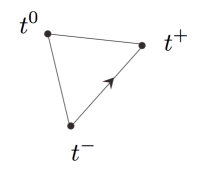
Figure 1. A perfect triangle

If ${\mathsf{G}}=\mathsf{SL}_{2}(\mathbb{R})$, then the perfect triangle associated to the standard ${\mathfrak{sl}_{2}}$-triple $(a_{0},x_{0},y_{0})$ described in equation (7) is $(0,\infty,1)$, the perfect triangle associated to $(a_{0},-x_{0},-y_{0})$ is $(0,\infty,-1)$. As a consequence

Definition 3.2.2.

[Vertices of a tripod] Let $\phi_{\tau}$ be the circle map associated to a tripod. The set of vertices associated to $\tau$ is the perfect triangle $\partial\tau\coloneqq\phi_{\tau}(0,\infty,1)$.

Observe that any triple of distinct points in a circle is a perfect triangle and that, if two tripods are coplanar, their vertices lie in the same circle.

3.2.1. Space of perfect triangles

The group ${\mathsf{G}}$ acts on the space of tripods, the space of ${\mathfrak{sl}_{2}}$-triples and the space of perfect triangles.

Proposition 3.2.3.

[Stabilizer of a perfect triangle] Let $t=(u,v,w)$ be a perfect triangle associated to a correct $\mathfrak{sl}_{2}$-triple $\mathfrak{s}$. Then the stabilizer of $t$ in ${\mathsf{G}}$ is the centralizer $\mathsf{Z}_{\mathfrak{s}}$ of $\mathfrak{s}$.

Proof.

Let $\xi$, $u$, $v$ and $w$ be as above. Denote by $L_{x,y}$ the stabilizer of a pair of transverse points $(x,y)$ in ${\bf F}$. Let also $A_{x,y}=L_{x,y}\cap\mathsf{S}$, where $\mathsf{S}$ is the group generated by $\mathfrak{sl}_{2}$ . Observe that $A_{x,y}$ is a 1-parameter subgroup. By Proposition 2.2.1, $L_{x,y}$ is the centralizer of $A_{x,y}$. Now given three distinct points in the projective line, the group generated by the three diagonal subgroups $A_{u,v}$, $A_{v,w}$ and $A_{u,w}$ is $\mathsf{SL}_{2}(\mathbb{R})$. Thus the stabilizer of a perfect triangle is the centralizer of $\mathfrak{s}$, that is $\mathsf{Z}_{\mathfrak{s}}$. ∎

Corollary 3.2.4.

1. The map $\mathfrak{s}\mapsto t_{\mathfrak{s}}$ defines a ${\mathsf{G}}$-equivariant homeomorphism from the space of correct triples to the space of perfect triangles.

2. We have $\mathcal{T}=\mathcal{G}/\mathsf{Z}_{0}$ and the map $\partial:\mathcal{G}\to\mathcal{T}$ is a (right) $\mathsf{Z}_{0}$-principal bundle.

A perfect triangle $t$, then defines a correct $\mathfrak{sl}_{2}$-triple and thus an homomorphism denoted $\xi^{t}$ from $\mathsf{SL}_{2}(\mathbb{R})$ to ${\mathsf{G}}$.

It will be convenient in the sequel to describe a tripod $\tau$ as a quadruple $(H,t^{-},t^{+},t^{0})$, where $t=(t^{-},t^{+},t^{0})\eqqcolon\partial\tau$ is a perfect triangle and $H$ is the set of all tripods coplanar to $\tau$. We write

$$\partial\tau=(t^{-},t^{+},t^{0}),\ \ \partial^{-}\tau=t^{-},\,\ \partial^{+}\tau=t^{+},\ \partial^{0}\tau=t^{0}.$$

3.3. Structures and actions

We have already described commuting left $\operatorname{Aut}({\mathsf{G}})$ and right $\operatorname{Aut}({\mathsf{G}}_{0})$ actions on $\mathcal{G}$ and in particular of $\mathsf{G}$ and $\mathsf{G}_{0}$.

Since $\mathsf{Z}_{0}$ is the centralizer of $\mathfrak{s}_{0}$, we also obtain a right action of $\mathsf{SL}_{2}(\mathbb{R})$ on $\mathcal{T}$, as well as a left ${\mathsf{G}}$-action, commuting together.

We summarize the properties of the actions (and specify some notation) in the following list.

1. Actions of ${\mathsf{G}}$ and ${\mathsf{G}}_{0}$

   1. the transitive left ${\mathsf{G}}$-action on $\mathcal{T}$ is given – in the interpretation of triangles – by $g(f_{1},f_{2},f_{3})\coloneqq(g(f_{1}),g(f_{2}),g(f_{3}))$. Interpreting, perfect triangles as morphisms $\xi$ from $\mathsf{SL}_{2}(\mathbb{R})$ to ${\mathsf{G}}$ in the class of $\rho$, then $(g\cdotp\xi)(x)=g\cdotp\xi(x)\cdotp g^{-1}$.

   2. The (right)-action of an element $b$ of ${\mathsf{G}}_{0}$ on $\mathcal{G}$ is denoted by $R_{b}$.

   We have the relation $R_{g}\cdotp\tau=\tau(g)\cdotp\tau$.

2. The right $\mathsf{SL}_{2}(\mathbb{R})$-action on $\mathcal{G}$ and $\mathcal{T}$ gives rises to a flow, an involution and an order 3 symmetry as follows;

   1. The shearing flow $\{\varphi_{s}\}_{s\in\mathbb{R}}$ is given by $\varphi_{s}\coloneqq R_{\exp(sa_{0})}$ on $\mathcal{G}$ . – See Figure (2(b)). if we denote by $\xi$ the embedding of $\mathsf{SL}(2,\mathbb{R})$ given by the perfect triangle $t=(t^{-},t^{+},t^{0})$, then

      $$\varphi_{s}(H,t^{-},t^{+},t^{0}) \coloneqq \left(H,t^{-},t^{+},\exp(sa)\cdotp t^{0})\right)\ ,$$

      where $a=\mathsf{T}\xi(a^{0})$ and $\mathsf{T}f$ denote the tangent map to a map $f$. We say that $\varphi_{R}(\tau)$ is $R$-sheared from $\tau$ .

   2. The reflection $\sigma:t\mapsto\overline{t}$ is given on $\mathcal{G}G$ by $\overline{\tau}=\tau\cdotp\sigma$, where $\sigma\in\mathsf{SL}_{2}(\mathbb{R})$ is the involution defined by $\sigma(\infty,0,1)=(0,\infty,-1)$. For the point of view of tripods via perfect triangles

      $$\overline{(H,t^{+},t^{-},t^{0})}=(H,t^{-},t^{+},s^{0})\ ,$$

      where $t^{-},t^{-},t^{0},s^{0}$ form a harmonic division on a circle – See Figure (2(b)). With the same notation the involution on $\mathcal{T}$ is given by $\overline{(t^{+},t^{-},t^{0})}=(t^{-},t^{+},s^{0})$.

   3. The rotation $\omega$ of order 3 – see Figure (2(a)) – is defined on $\mathcal{G}$ by $\omega(\tau)=\tau\cdotp r_{\omega}\ .$ where $r_{\omega}\in\mathsf{PSL}_{2}(\mathbb{R})$ is defined by $r_{\omega}(0,1,\infty)=(1,\infty,0)$. For the point of view of tripods via perfect triangles

      $$\omega(H,t^{-},t^{+},t^{0})=(H,t^{+},t^{0},t^{-})\ ,$$

      Similarly the action of $\omega$ on $\mathsf{T}$ is given by $\omega(t^{-},t^{+},t^{0})=(t^{+},t^{0},t^{-})$.

3. Two foliations ${\mathcal{U}}^{-}$ and ${\mathcal{U}}^{+}$ on $\mathcal{G}$ and $\mathcal{T}$ called respectively the stable and unstable foliations. The leaf of ${\mathcal{U}}^{\pm}$ is defined as the right orbit of respectively $\mathsf{N}^{+}_{0}$ and $\mathsf{N}^{-}_{0}$ (normalized by $Z_{0}$) and alternatively by

   $${\mathcal{U}}^{\pm}_{\tau}:=\mathsf{U}^{\pm}(\tau),$$

   where ${\mathsf{U}}^{\pm}(\tau)$ is the unipotent radical of the stabilizer of $\partial^{\pm}\tau$ under the left action of ${\mathsf{G}}$. We also define the central stable and central unstable foliations by the right actions of respectively $\mathsf{P}^{\pm}_{0}$ or alternatively by

   $${\mathcal{U}}^{\pm,0}_{\tau}:={\mathsf{U}}^{\pm,0}(\tau),$$

   where ${\mathsf{U}}^{\pm,0}(t)$ is the stabilizer of $\partial^{\pm}\tau$ under the left action of ${\mathsf{G}}$. Observe that ${\mathsf{U}}^{\pm,0}(t)$ are both conjugate to $\mathsf{P}_{0}$.

4. A foliation, called the central foliation, $\mathcal{L}^{0}$ whose leaves are the right orbits of $\mathsf{L}_{0}$ on $\mathcal{G}$, naturally invariant under the action of the flow $\{\varphi_{s}\}_{s\in\mathbb{R}}$. Alternatively,

   $${\mathcal{L}}^{0}_{\tau}={\mathsf{L}}^{0}(\tau),$$

   where ${\mathsf{L}}^{0}(\tau)$ is the stabilizer in ${\mathsf{G}}$ of $(\partial^{+}\tau,\partial^{-}\tau)$.

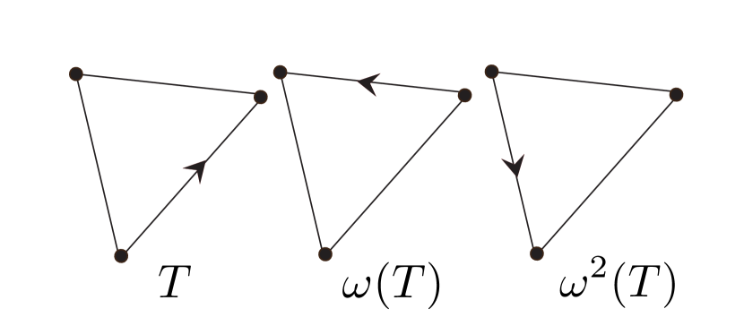
(a) Permutation of order 3

(b) Flow and involution

Figure 2. Some actions

Then we have

Proposition 3.3.1.

The following properties hold:

1. the action of ${\mathsf{G}}$ commutes with the flow $\{\varphi_{s}\}_{s\in\mathbb{R}}$, the involution $\sigma$ and the permutation $\omega$.

2. For any real number $s$ and tripod $\tau$, $\overline{\varphi_{s}(\tau)}=\varphi_{-s}(\overline{\tau})$.

3. The foliations ${\mathcal{U}}^{+}$ and ${\mathcal{U}}^{-}$ are invariant by the left action of ${\mathsf{G}}$.

4. Moreover the leaves of ${\mathcal{U}}^{+}$ and ${\mathcal{U}}^{-}$ on $\mathcal{G}$ are respectively uniformly contracted (with respect to any left ${\mathsf{G}}$-invariant Riemannian metric) and dilated by the action of $\{R_{\exp(tu)}\}_{t\in\mathbb{R}}$ for $u$ in the interior of the positive Weyl chamber and $t>0$.

5. The flow $\{\varphi_{t}\}_{t\in\mathbb{R}}$ acts by isometries along the leaves of $\mathcal{L}_{0}$.

6. We have $\tau\in{\mathcal{U}}^{0,-}_{\eta}$ if and only if $\partial^{-}\tau=\partial^{-}\eta$.

Proof.

The first three assertions are immediate.

Let us choose a tripod $\tau$ so that $\mathcal{G}$ is identified respectively with ${\mathsf{G}}=\mathsf{G}_{0}$ . If $d$ is a left invariant metric associated to a norm $\|\cdotp\|$ on $\mathfrak{g}$, the image of $d$ under the right action of an element $g$ is associated to the norm $\|\cdotp\|_{g}$ so that $\|u\|_{g}=\|\operatorname{ad}(g)\cdotp u\|$. The fourth and fifth assertion follow from that description.

For the last assertion, ${\mathcal{U}}^{0,-}_{\tau}={\mathcal{U}}^{0,-}_{\sigma}$, if and only if the stabilizer of $\partial^{-}\tau$ and $\partial^{-}\sigma$ are the same. The result follows ∎

Corollary 3.3.2.

[Contracting along leaves] For any left invariant Riemannian metric $d$ on $\mathsf{G}$, there exists a constant ${{\bf M}}$ only depending on $\mathsf{G}$ so that if $\varepsilon$ is small enough, then for all positive $R$, the following two properties hold

$$d(u,v)\leqslant\varepsilon\ ,\ d(\varphi_{R}(u),\varphi_{R}(v))\leqslant\varepsilon \implies \forall t\in[0,R],\ d(\varphi_{t}(u),\varphi_{t}(v))\leqslant{{\bf M}}\varepsilon\ ,$$

$$\partial^{-}u=\partial^{-}v,\ d(u,v)\leqslant\varepsilon \implies \forall t<0,\ d(\varphi_{t}(u),\varphi_{t}(v))\leqslant{{\bf M}}\varepsilon\ .$$

3.3.1. A special map

We consider the map $K$ – see Figure (3) – defined from $\mathcal{T}$ or $\mathcal{G}$ to itself by

$$K(x):={\omega(\overline{x})}.$$

Figure 3. The map $K$

Later on, we shall need the following property of this map $K$.

Proposition 3.3.3.

For any $(x,y,z)$ in $\mathcal{T}$, $K(x,y,z)=(x,t,y)$ for some $t$ in ${\bf F}$. The map $K$ preserves each leaf of the foliation ${\mathcal{U}}^{0,-}$.

Proof.

This follows from the point (vi) in Proposition 3.3.1. ∎

3.4. Tripods, measures and metrics

Let us equip once and for all $\mathcal{G}$ with a Riemannian metric $d$ invariant under the left action of $\mathsf{G}$, as well as the action of $\omega$. We will denote by $d_{0}$ the metric on $\mathsf{G}_{0}$ so that $d(\tau\cdotp g,\tau\cdotp h)=d_{0}(g,h)$ for all tripods $\tau$ and observe that $d_{0}$ is left invariant. The associated Lebesgue measure is now both left invariant by $\operatorname{Aut}(\mathsf{G})$ and right invariant by $\operatorname{Aut}(\mathsf{G}_{0})$.

We denote by $\operatorname{Sym}({\mathsf{G}})$ the symmetric space of ${\mathsf{G}}$ seen as the space of Cartan involutions of $\mathfrak{g}$. Let us first recall some facts about the totally geodesic space $\operatorname{Sym}({\mathsf{G}})$.

Let $\mathsf{H}$ be a subgroup of $\mathsf{G}$. The $\mathsf{H}$-orbit of a Cartan involution $i$, so that $i(\mathfrak{h})=\mathfrak{h}$, is a totally geodesic subspace of $\operatorname{Sym}(\mathsf{G})$ isometric to $\operatorname{Sym}(\mathsf{H})$ – we then say of type $\mathsf{H}$.

Any two totally geodesic spaces $H_{1}$ and $H_{2}$ of the same type are parallel: that is for all $x_{i}\in H_{i}$, $\inf(d(x_{i},y)\mid y\in H_{i+1})$ is constant and equal by definition to the distance $h(H_{1},H_{2})$.

The space of parallel totally geodesic subspaces to a given one is isometric to $\operatorname{Sym}(\mathsf{Z})$ if $\mathsf{Z}$ is the centralizer of $\mathsf{H}$, and in particular reduced to a point if $\mathsf{Z}$ is compact.

3.4.1. Totally geodesic hyperbolic planes

By assumption (8), if $\tau$ is a tripod, the Cartan involution

$${\boldsymbol{i}}_{\tau}\coloneqq\tau\circ{\boldsymbol{i}}_{0}\circ\tau^{-1}$$

send the correct ${\mathfrak{sl}_{2}}$-triple $(a,x,y)$ associated to the tripod $\tau$ to $(-a,y,x)$. It follows that the image of a right $\mathsf{SL}_{2}(\mathbb{R})$-orbit gives rise to a totally geodesic embedding of the hyperbolic plane denoted $\eta_{\tau}$ and that we call correct and which is equivariant under the action of a correct $\mathsf{SL}_{2}(\mathbb{R})$.

Observe also that a totally geodesic embedding of ${\bf H}^{2}$ in $\operatorname{Sym}({\mathsf{G}})$ is the same thing as a totally geodesic hyperbolic plane $H$ in $\operatorname{Sym}({\mathsf{G}})$ with three given points in the boundary at infinity in $H$.

Let us consider $\mathcal{H}$ the space of correct totally geodesic maps from ${\bf H}^{2}$ to the symmetric space $\operatorname{Sym}({\mathsf{G}})$.

Proposition 3.4.1.

The space $\mathcal{H}$ is equipped with a transitive action of $\operatorname{Aut}(\mathsf{G})$ and a right action of $\mathsf{SL}_{2}(\mathbb{R})$.

We have also have $\mathsf{SL}_{2}(\mathbb{R})\times{\mathsf{G}}$ equivariant maps

$$\mathcal{G}\to\mathcal{H}\to\mathcal{T},$$ (9)

$$\tau\mapsto\eta_{\tau}\mapsto\partial\tau$$ (10)

so that the composition is the map $\partial$ which associates to a tripod its vertices. Moreover if the centralizer of the correct $\mathfrak{sl}_{2}$-triple is compact then $\mathcal{H}=\mathcal{T}$.

Proof.

We described above that map $\tau\mapsto\eta_{\tau}$. By construction this map is $\mathsf{SL}_{2}(\mathbb{R})\times{\mathsf{G}}$ equivariant.The map $\partial$ from $\mathcal{G}$ to $\mathcal{T}$ obviously factors through this map.

If the centralizer of a correct $\mathsf{SL}_{2}(\mathbb{R})$ in $\mathsf{G}$, is compact then all correct parallel hyperbolic planes are identical. The result follows. ∎

From this point of view, a tripod $\tau$ defines

1. A totally geodesic hyperbolic plane ${\bf H}^{2}_{\tau}$ in $S({\mathsf{G}})$, with three preferred points denoted $\tau(0),\tau(\infty),\tau(1)$ in $\partial_{\infty}{\bf H}^{2}_{\tau}$,

2. An $\mathsf{SL}_{2}(\mathbb{R})$-equivariant map $\phi^{\tau}$ from $\partial_{\infty}{\bf H}^{2}_{\tau}$ to ${\bf F}$, so that

   $$\phi^{\tau}\left((\tau(0),\tau(\infty),\tau(1)\right)=\partial\tau.$$

3.4.2. Metrics, cones, and projection on the symmetric space

Definition 3.4.2.

[Projection and metrics] We define the projection from $\mathcal{G}$ to $\operatorname{Sym}({\mathsf{G}})$ to be the map

$$s:\tau\mapsto s(\tau)\coloneqq\eta_{\tau}(i)\ .$$

In other words, $s(\tau)$ is the orthogonal projection of $\tau(1)$ on the geodesic $]\tau(0),\tau(\infty)[$ – see figure (4).

Figure 4. Projection

The metric on $\mathfrak{g}$ associated to $s(\tau)$ is denoted by $d_{\tau}$ and so are the associated metrics on ${\bf F}$ – seeing ${\bf F}$ as a subset of the Grassmannian of $\mathfrak{g}$ – and the right invariant metric on ${\mathsf{G}}$ defined by

$$d_{\tau}(g,h)=\sup\{d_{\tau}(g(x),h(x))\mid x\in{\bf F}\}.$$ (11)

As a particular case, a triple $\tau$ of three pairwise distinct points in ${\bf P}^{1}(\mathbb{R})$ defines a metric $d_{\tau}$ on ${\bf P}^{1}(\mathbb{R})$ – So that ${\bf P}^{1}(\mathbb{R})$ is isometric to $S^{1}$ – that is called the visual metric of $\tau$. The following properties of the assignment $\tau\mapsto d_{\tau}$, for $d_{\tau}$ a metric on ${\bf F}$ will be crucial

1. For every $g$ in ${\mathsf{G}}$, $d_{g\tau}(g(x),g(y))=d_{\tau}(x,y)$,

2. The circle map associated to any tripod $\tau$ is an isometry from ${\bf P}^{1}(\mathbb{R})$ equipped with the visual metric of $(0,1,\infty)$ to ${\bf F}$ equipped with $d_{\tau}$.

3.4.3. Elementary properties

Proposition 3.4.3.

We have

1. For all tripod $\tau$: $d_{\tau}=d_{\overline{\tau}}$.

2. If the stabilizer of $\mathfrak{s}$ is compact, $d_{\tau}$ only depends on $\partial\tau$.

Proof.

The first item comes from the fact that $d_{\tau}$ only depends on $s(\tau)$. For the second item, in that case the map $\eta_{\tau}\mapsto\partial_{\tau}$ is an isomorphism, by Proposition 3.4.1. ∎

Proposition 3.4.4.

[Metric equivalences] For every positive numbers $A$ and $\varepsilon$, there exists a positive number $B$ so that if $\tau,\tau^{\prime}\in\mathcal{T}$ are tripods and $g\in{\mathsf{G}}$, then

$$d_{\tau}(g,\operatorname{Id})\leqslant\varepsilon\hbox{ and }d(\tau,\tau^{\prime})\leqslant A\implies d_{\tau}(g,\operatorname{Id})\leqslant B\cdotp d_{\tau^{\prime}}(g,\operatorname{Id})\ .$$

Similarly, for all $u,v$ in ${\bf F}$ and $g\in\mathsf{G}$

$$d(\tau,\tau^{\prime})\leqslant A \implies d_{\tau}(u,v)\leqslant B\cdotp d_{\tau^{\prime}}(u,v)\ ,$$ (12)

$$d(\tau,g\tau)\leqslant\varepsilon \implies d_{\tau}(g,\operatorname{Id})\leqslant B\cdotp d(\tau,g\tau)\ ,$$ (13)

Proof.

Let $U(\varepsilon)$ be a compact neighborhood of $\operatorname{Id}$. The ${\mathsf{G}}$-equivariance of the map $d:\tau\mapsto d_{\tau}$ implies the continuity of $d$ seen as a map from $\mathcal{G}$ to $C^{1}(U(\varepsilon)\times U(\varepsilon))$ – equipped with uniform convergence. The first result follows. The second assertion follows by a similar argument. For the inequality (13), let us fix a tripod $\tau_{0}$. The metrics

$$(g,h)\mapsto d_{\tau_{0}}(g,h),\ \ (g,h)\mapsto d(h^{-1}\cdotp\tau_{0},g^{-1}\cdotp\tau_{0})\ ,$$

are both right invariant Riemannian metrics on ${\mathsf{G}}$. In particular, they are locally bilipschitz and thus there exists some $B$ so that

$$d(\tau_{0},g\tau_{0})\leqslant\varepsilon\implies d_{\tau_{0}}(g,\operatorname{Id})\leqslant B\cdotp d(g_{0}^{-1}\cdotp\tau_{0},\tau_{0})=B\cdotp d(\tau_{0},g\cdotp\tau_{0})\ .$$

We now propagate this inequality to any tripod using the equivariance: writing $\tau=h\cdotp\tau_{0}$, we get that assuming $d(\tau,g\cdotp\tau)\leqslant\varepsilon$, then

$$d(\tau_{0},h^{-1}gh\cdotp\tau_{0})=d(h\cdotp\tau_{0},gh\cdotp\tau)=d(\tau,g\cdotp\tau)\leqslant\varepsilon\ .$$

Thus according to the previous implication,

$$d_{\tau_{0}}(h^{-1}gh,\operatorname{Id})\leqslant B\cdotp d(\tau_{0},h^{-1}gh\cdotp\tau_{0})=B\cdotp d(\tau,g\cdotp\tau)\ .$$

The result follows from the equalities $d_{\tau_{0}}(h^{-1}gh,\operatorname{Id})=d_{h\cdotp\tau_{0}}(gh,h)=d_{\tau}(g,\operatorname{Id}).$ ∎

As a corollary

Corollary 3.4.5.

[$\omega$ is uniformly Lipschitz] There exists a constant $C$ so that for all $\tau$

$$\frac{1}{C}d_{\tau}\leqslant d_{\omega(\tau)}\leqslant C\cdot d_{\tau}\ .$$

3.4.4. Aligning tripods

We explain a slightly more sophisticated way to control tripod distances.

Let $\tau_{0}$ and $\tau_{1}$ be two coplanar tripods associated to a totally geodesic hyperbolic plane ${\bf H}^{2}$ and a circle $C$ identified with $\partial_{\infty}{\bf H}^{2}$ so that $z_{1},z_{0}\in C$. We say that $(z_{0},\tau_{0},\tau_{1},z_{1})$ are aligned if there exists a geodesic $\gamma$ in ${\bf H}^{2}$, passing through $s(\tau_{0})$ and $s(\tau_{1})$ starting at $z_{0}$ and ending in $z_{1}$. In the generic case $s(\tau_{0})\not=s(\tau_{1})$, $z_{1}$ and $z_{0}$ are uniquely determined.

We first have the following property which is standard for ${\mathsf{G}}=\mathsf{SL}(2,\mathbb{R})$,

Proposition 3.4.6.

[Aligning tripods] There exist positive constants $\boldsymbol{K}$, $c$ and $\alpha_{0}$ only depending on ${\mathsf{G}}$ so that if $(z_{0},\tau_{0},\tau_{1},z_{1})$ are aligned and associated to a circle $C\subset{\bf F}$ the following holds: Let $w\in C$ satisfying $d_{\tau_{1}}\left(w,z_{1}\right)\leqslant 3\pi/4$, then we have

$$d_{\tau_{1}}(w,u)\leqslant\alpha_{0}\ ,\ d_{\tau_{1}}(w,v)\leqslant\alpha_{0}\implies d_{\tau_{0}}(u,v)\leqslant\frac{\boldsymbol{K}}{4}e^{-cd(\tau_{0},\tau_{1})}\cdot d_{\tau_{1}}(u,v)\ .$$ (14)

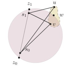
Figure 5. Aligning tripods

Proof.

There exists a correct ${\mathfrak{sl}_{2}}$-triple $s=(a,x,y)$ preserving the totally geodesic plane ${\bf H}^{2}_{\tau_{0}}$ so that the 1-parameter group $\{\lambda_{t}\}_{t\in\mathbb{R}}$ generated by $a$ fixes $C$ and has $z_{1}$ as an attractive fixed point and $z_{0}$ as a repulsive fixed point in ${\bf F}$. Let $t_{1}$ the positive number defined by $\lambda_{t_{1}}(s(\tau_{0}))=s(\tau_{1})$.

Recall that by construction $d_{\tau}$ only depends on $s(\tau)$. Let $B\subset C$ be the closed ball of center $z_{1}$ and radius $3\pi/4$ with respect to $d_{\tau_{1}}$. Observe that $B$ lies in the basin of attraction of $H$ and so does $U$ a closed neighborhood of $B$. In particular, we have that the 1-parameter group $H$ converges $C^{1}$-uniformly to a constant on $U$. Thus,

$$\exists K_{0},d>0,\ \ \forall u,v\in U,\ \ \forall t\geqslant 0, \ d_{\tau_{1}}(\lambda_{t}(u),\lambda_{t}(v))\leqslant K_{0}e^{-dt}\cdotp d_{\tau_{1}}(u,v)\ .$$ (15)

Recall that for all $u,v$ in ${\bf F}$, since $s\left(\lambda_{-t_{1}}(\tau_{1})\right)=s(\tau_{0})$.

$$d_{\tau_{1}}(\lambda_{t_{1}}(u),\lambda_{t_{1}}(u))=d_{\lambda_{-t_{1}}(\tau_{1})}(u,v)=d_{\tau_{0}}(u,v)$$ (16)

Finally, there exists $\alpha>0$, only depending on ${\mathsf{G}}$ so that for any $w$ in $B$, the ball $B_{w}$ of radius $\alpha$ with respect to $d_{\tau_{1}}$ lies in $U$. Thus, combining (15) and (16) we get

$$d_{\tau_{0}}(u,v)\leqslant K_{0}\cdotp e^{-dt}d_{\tau_{1}}(u,v).$$

This concludes the proof of Statement (14) since there exists constants $B$ and $C$ so that $d(\tau_{0},\tau_{1})\leqslant Bt_{1}+C$. ∎

3.5. The contraction and diffusion constants

The constant $\boldsymbol{K}$ defined in Proposition 3.4.6 will be called the diffusion constant and $\boldsymbol{\kappa}:=\boldsymbol{K}^{-1}$ is called the contraction constant.

4. Quasi-tripods and finite paths of quasi-tripods

We now want to describe a coarse geometry in the flag manifold; our main devices will be the following: paths of quasi-tripods and coplanar paths of tripods. Since not all triple of points lie in a circle in ${\bf F}$, we need to introduce a deformation of the notion of tripods. This is achieved through the definition of quasi-tripod 4.1.1.

A coplanar path of tripods is just a sequence of non overlapping ideal triangles in some hyperbolic plane such that any ideal triangle have a common edge with the next one. Then a path of quasi-tripods is a deformation of that, such a path can also be described as a model which is deformed by a sequence of specific elements of ${\mathsf{G}}$.

Our goal is the following. The common edges of a coplanar path of tripods, considered as intervals in the boundary at infinity of the hyperbolic plane, defines a sequence of nested intervals. We want to show that in certain circumstances, the corresponding chords of the deformed path of quasi-tripods are still nested in the deformed sense that we introduced in the following sections.

One of our main result is then the Confinement Lemma 6.0.1 which guarantees squeezing.

4.1. Quasi-tripods

Quasi-tripods will make sense of the notion of a “deformed ideal triangle” . Related notions are defined: swished quasi-tripods, and the foot map.

Definition 4.1.1.

[Quasi-tripods] An $\varepsilon$-quasi tripod is a quadruple $\theta=(\accentset{\mbox{\large.}}{\theta},\theta^{-},\theta^{+},\theta^{0})\in\mathcal{G}\times{\bf F}^{3}$ so that

$$d_{\accentset{\mbox{\large.}}{\theta}}(\partial^{+}\accentset{\mbox{\large.}}{\theta},\theta^{+}))\leqslant\varepsilon\ ,\ d_{\accentset{\mbox{\large.}}{\theta}}(\partial^{-}\accentset{\mbox{\large.}}{\theta},\ \ \theta^{-}))\leqslant\varepsilon\ ,\ \ d_{\accentset{\mbox{\large.}}{\theta}}(\partial^{0}\accentset{\mbox{\large.}}{\theta},\theta^{0})\leqslant\varepsilon\ .$$

The set $\partial\theta\coloneqq\{\theta^{+},\theta^{-},\theta^{0}\}$ is the set of vertices of $\theta$ and $\accentset{\mbox{\large.}}{\theta}$ is the interior of $\theta$ . An $\varepsilon$-quasi tripod $\tau$ is reduced if $\partial^{\pm}\accentset{\mbox{\large.}}{\tau}=\tau^{\pm}$.

Obviously a tripod defines an $\varepsilon$-quasi tripod for all $\varepsilon$. Moreover, some of the actions defined on tripods in paragraph 3.3 extend to $\varepsilon$-quasi tripods, most notably, we have an action of a cyclic permutation $\omega$ of order three on the set of quasi-tripods, given by

$$\omega(\accentset{\mbox{\large.}}{\theta},\theta^{-},\theta^{+},\theta^{0})=(\omega(\accentset{\mbox{\large.}}{\theta}),\theta^{+},\theta^{0},\theta^{-})\ .$$

By Corollary 3.4.5,

Proposition 4.1.2.

There is a constant ${{\bf M}}$ only depending on $\mathsf{G}$, such that if $\theta$ is an $\varepsilon$-quasi tripod then, $\omega(\theta)$ is an ${{\bf M}}\varepsilon$-quasi tripod

4.1.1. A foot map

For any positive $\beta$, let us consider the following $\mathsf{G}$-stable set

$$W_{\beta}\coloneqq\{(\tau,a^{+},a^{-})\mid\tau\in\mathcal{G},a^{\pm}\in{\bf F},\,\,d_{\tau}(a^{\pm},\partial^{\pm}\tau)\leqslant\beta\}\subset\mathcal{G}\times{\bf F}^{2}.$$

Lemma 4.1.3.

There exists positive numbers $\beta$ and ${{\bf M}}_{1}$, a smooth $\mathsf{G}$-equivariant map $\Psi:W_{\beta}\to\mathcal{G}$, so that

1. $\partial^{\pm}\Psi(\tau,a^{+},a^{-})=a^{\pm}$,

2. $d(\tau,\Psi(\tau,a^{+},a^{-}))\leqslant M\cdotp\sup(d_{\tau}(a^{\pm},\partial^{\pm}\tau))$.

3. $\Psi$ is ${{\bf M}}_{1}$-Lipschitz.

Proof.

For a transverse pair $a=(a^{+},a^{-})$ in ${\bf F}$, let $\mathcal{G}_{a}$ be the set of tripods $\tau$ in $\mathcal{G}$ so that $\partial^{\pm}\tau=a^{\pm}$ and $\mathsf{G}_{a}$ the stabilizer of the pair $a^{+}$, $a^{-}$. Let us fix (in a ${\mathsf{G}}$-equivariant way) a small enough tubular neighborhood $N_{a}$ of $\mathcal{G}_{a}$ in $\mathcal{G}$ for all transverse pairs $a=(a^{+},a^{-})$ as well as a ${\mathsf{G}}_{a}$-equivariant projection $\Pi_{a}$ from $N_{a}$ to $\mathcal{G}_{a}$. By continuity one gets that for $\beta$ small enough, if $(\tau,a^{+},a^{-})\in W_{\beta}$ then $\tau\in N_{a}$. We now define

$$\Psi(\tau,a^{+},a^{-})\coloneqq\Pi_{a}(\tau)\ .$$

By $\mathsf{G}$-equivariance, $\Psi$ is uniformly Lipschitz. ∎

Definition 4.1.4.

[Foot map and feet] A map $\Psi$ satisfying the conclusion of the lemma is called a foot map. For $\varepsilon$ small enough, we define the feet $\psi_{1}(\theta)$, $\psi_{2}(\theta)$ and $\psi_{3}(\theta)$ of the $\varepsilon$-quasi tripod $\theta=(\accentset{\mbox{\large.}}{\theta},\theta^{-},\theta^{+},\theta^{0})$ as the three tripods which are respectively defined by

$$\psi_{1}(\theta)\coloneqq\Psi\left(\accentset{\mbox{\large.}}{\theta},\theta^{-},\theta^{+}\right)\ ,\ \psi_{2}(\theta)\coloneqq\psi_{1}(\omega(\theta))\ ,\ \psi_{3}(\theta)\coloneqq\psi_{1}(\omega^{2}(\theta))\ .$$

Where $\Psi$ is the foot map defined in the preceding section.

By the last item of Lemma 4.1.3, for an $\varepsilon$, quasi tripod $\theta$

$$d\left(\psi_{i}(\theta),\omega^{i-1}\left(\accentset{\mbox{\large.}}{\theta}\right)\right)\leqslant{{\bf M}}_{1}\varepsilon\ ,$$ (17)

Observe also that, for $\varepsilon$ small enough there exists a constant ${{\bf M}}_{2}$ only depending on ${\mathsf{G}}$, so that for $\varepsilon$ small enough if $\theta$ is an $\varepsilon$-quasi tripod then

$$d(\omega(\psi_{1}(\theta)),\psi_{2}(\theta))\leqslant{{\bf M}}_{2}\varepsilon\ ,\ d(\omega(\psi_{2}(\theta)),\psi_{3}(\theta))\leqslant{{\bf M}}_{2}\varepsilon\ .$$ (18)

Using the triangle inequality, this is a consequence of the previous inequality and the assumption that $\omega$ is an isometry for $d$.

4.1.2. Foot map and flow

The following property explains how well the foot map behaves with respect to the flow action.

Proposition 4.1.5.

[Foot and flow]

There exists positive constants $\beta_{1}$ and ${{\bf M}}_{3}$ with the following property. Let $\varepsilon\leqslant\beta_{1}$, let $x_{0}$ in $\mathcal{G}$, $x_{1}:=\varphi_{R}(x_{0})$ for some $R$. Let $a=(a^{+},a^{-})$ be a transverse pair of flags ${\bf F}$, so that $d_{x_{i}}(a^{\pm},\partial^{\pm}x_{i})\leqslant\varepsilon$, then

$$d(y_{1},\varphi_{R}(y_{0}))\leqslant{{\bf M}}_{3}\varepsilon\ ,$$

where $y_{i}=\Psi(x_{i},a^{+},a^{-})$.

Proof.

In the proof $M_{i}$ will denote a constant only depending on $\mathsf{G}$.

It is enough to prove the weaker result that there exists $z_{0}$, $z_{1}=\varphi_{R}(z_{0})$ in $\mathcal{G}_{a}$ so that $d(z_{i},x_{i})\leqslant M_{7}\varepsilon$. Indeed, it first follows that $d(z_{i},y_{i})\leqslant M_{8}\varepsilon$ by the triangle inequality. Secondly, $\mathsf{G}_{a}$ is a central leaf of the foliation and the flow acts by isometries on it (see Property (v) of Proposition 3.3.1), it then follows that $d(y_{1},\varphi_{R}(y_{0}))\leqslant M_{9}\varepsilon$ and the result follows

Observe first that $d(x_{i},y_{i})\leqslant M\varepsilon$ by definition of a foot map. Assume $R>0$. Let $x^{\pm}=\partial^{\pm}x_{0}=\partial^{\pm}x_{1}$. Let us first assume that $x^{+}=a^{+}$. Thus by the contraction property

$$d(\varphi_{R}(x_{0}),\varphi_{R}(y_{0}))\leqslant M_{2}\varepsilon\ .$$

It follows by the triangle inequality that

$$d(\varphi_{R}(y_{0}),y_{1})\leqslant M_{3}\varepsilon\ .$$

Thus this works with $z_{0}=y_{0}$, $z_{1}=\varphi_{R}(z_{0})$.

The same results hold symmetrically whenever $x^{-}=a^{-}$ by taking $z_{1}=y_{1}$, $z_{0}=\varphi_{-R}(z_{1})$.

The general case follows by considering intermediate projections. First (as a consequence of our initial argument) we find $w_{0}$ and $w_{1}=\varphi_{R}(w_{0})$ in $\mathcal{G}_{a^{+},x^{-}}$ with $d(w_{i},x_{i})\leqslant M_{3}\varepsilon$.

Applying now the symmetric argument with the pair $w_{0}$, $w_{1}$ and projection on $\mathcal{G}_{a^{+},x^{-}}$ we get $z_{0}$ and $z_{1}:=\varphi_{R}(z_{0})$ so that $d(w_{i},z_{i})\leqslant M_{3}\varepsilon$.

A simple combination of triangle inequalities yield the result. ∎

4.1.3. Swishing quasi-tripods

Definition 4.1.6.

[Swishing quasi-tripods] The $\varepsilon$-quasi-tripod $\theta^{\prime}$ is $(R,\alpha)$-swished from the $\varepsilon$-quasi tripod $\theta$ if

1. $\partial^{\pm}\theta=\partial^{\mp}\theta^{\prime}$.

2. The tripods $\psi_{1}(\theta^{\prime})$ and $\overline{\varphi_{R}(\psi_{1}(\theta))}$ are $\alpha$-close.

Being swished is a reciprocal condition:

Proposition 4.1.7.

If $\theta^{\prime}$ is $(R,\alpha)$-swished from $\theta$, then $\theta$ is $(R,\alpha)$-swished from $\theta^{\prime}$.

Proof.

We have $d(\sigma(\varphi_{R}(\theta)),\theta^{\prime})=d(\varphi_{R}(\theta),\sigma(\theta^{\prime}))$. Since $\partial^{\pm}\theta=\partial^{\mp}\theta^{\prime}$, $\sigma(\theta^{\prime})=(\theta)g$ for some $g\in L_{0}$. Since by Proposition 3.3.1 (v), $\varphi_{R}$ acts by isometries on the orbits of $\mathsf{L}_{0}$, we get

$$d(\sigma(\varphi_{R}(\theta)),\theta^{\prime})=d(\varphi_{R}(\theta),\sigma(\theta^{\prime}))=d\left(\theta,\varphi_{-R}\left(\sigma(\theta^{\prime})\right)\right).$$

But, by Proposition 3.3.1 again, $\varphi_{-R}\circ\sigma=\sigma\circ\varphi_{R}$. The result follows. ∎

4.2. Paths of quasi-tripods and coplanar paths of tripods

(a) coplanar path of tripods

(b) path of reduced quasi-tripods

Figure 6. A deformation of a path of quasi-tripods

4.2.1. Swished paths of quasi-tripods and their model

Let $\underline{R}(N)=(R_{0},\ldots,R_{N})$ be a finite sequence of positive numbers.

Definition 4.2.1.

[coplanar paths of tripods] An $\underline{R}(N)$-swished coplanar path of tripods is a sequence of tripods $\underline{\tau}(N)=(\tau_{0},\ldots\tau_{N})$ such that $\tau_{i+1}$ is $R_{i}$-swished from $\omega^{n_{i}}\tau_{i}$, where $n_{i}\in\{1,2\}$. The sequence $(n_{1},\ldots,n_{N})$ is the combinatorics of the path.

We remark that a coplanar path of tripods consists of pairwise coplanar tripods and is totally determined up to the action of ${\mathsf{G}}$ by $\underline{R}(N)$ and the combinatorics. These coplanar paths of tripods will represent the model situation and we need to deform them.

Definition 4.2.2.

[paths of quasi-tripods] An $(\underline{R}(N),\varepsilon)$-swished path of quasi-tripods is a sequence of $\varepsilon$-quasi tripods $\underline{\theta}(N)=(\theta_{0},\ldots\theta_{N})$, and such that $\theta_{i+1}$ is $(R_{i},\varepsilon)$-swished from $\omega^{n_{i}}\theta_{i}$, where $n_{i}\in\{1,2\}$. The sequence $(n_{1},\ldots,n_{N})$ is the combinatorics of the path.

A model of an $(\underline{R}(N),\varepsilon)$-swished path of quasi-tripods is an $\underline{R}(N)$-swished coplanar path of tripods with the same combinatorics.

Let us introduce some notation and terminology: $\partial\theta_{i}$, $\partial\theta_{i+1}$ and $\partial\theta_{i-1}$ have exactly one point in common denoted $x_{i}$ and called the pivot of $\theta_{i}$. Remarks: Observe that given a path of quasi-tripods,

1. There exists some constant $M$, so that any $(\underline{R}(N),\varepsilon)$-swished path of quasi-tripods give rise to an $(\underline{R}(N),M\varepsilon)$-swished path of quasi-tripods with the same vertices but which are all reduced. In the sequel, we shall mostly consider such reduced paths of quasi-tripods.

2. From the previous items, in the case of reduced path, the sequence of triangles $(\theta_{0},\ldots,\theta_{N})$ is actually determined by the sequence of (not necessarily coplanar) tripods $(\accentset{\mbox{\large.}}{\theta_{0}},\ldots,\accentset{\mbox{\large.}}{\theta_{N}})$.

One immediately have

Proposition 4.2.3.

Any $(\underline{R}(N),\varepsilon)$-swished path of quasi-tripods admits a model which is unique up to the action of ${\mathsf{G}}$.

4.2.2. Coplanar paths of tripods and sequence of chords

To a reduced path of quasi-tripods $\underline{\theta}(N)$ we associate a path of chords

$$\underline{h}(N)=(h_{0},\ldots,h_{N})$$

such that $h_{i}\coloneqq h_{\accentset{\mbox{\large.}}{\theta_{i}}}$ has $x_{i}$ and $x^{i}$ as extremities. Observe, that the subsequence of triangles $(\theta_{0},\ldots,\theta_{N-1})$ is actually determined by the sequence of chords $(h_{0},\ldots,h_{N})$.

In the sequel, by an abuse of language, we shall call the sequence of chords $\underline{h}(N)$ a path of quasi-tripods as well.

Observe that for a coplanar path of tripods the associated path of chords is so that $(h_{i},h_{i+1})$ is nested.

4.2.3. Deformation of coplanar paths of tripods

Let $\underline{\tau}=(\tau_{0},\ldots,\tau_{N})$ be a coplanar path of tripods.

Definition 4.2.4.

[Deformation of paths] A deformation of $\underline{\tau}$ is a sequence $v=(g_{0},\ldots,g_{N_{1}})$ with $g_{i}\in\mathsf{P}_{x_{i}}$, the stabilizer of $x_{i}$ in ${\mathsf{G}}$, where $x_{i}$ is the pivot of $\tau_{i}$. The deformation is an $\varepsilon$-deformation if furthermore $d_{\tau_{i}}(g_{i},\operatorname{Id})\leqslant\varepsilon$.

Given a deformation $v=(g_{0},\ldots,g_{N-1})$, the deformed path of quasi-tripods is the path of quasi-tripods $\underline{\theta}^{v}=(\theta_{0}^{v},\ldots,\theta_{N}^{v})$ where

for $$i<N, \,\theta_{i}^{v}=(b_{i}\tau_{i},b_{i}\tau_{i}^{-},b_{i}\tau_{i}^{+},b_{i+1}\tau_{i}^{0}),$$ (19)

for $$i=N, \,\theta_{N}^{v}=(b_{N}\tau_{N},b_{N}\tau_{N}^{-},b_{N}\tau_{N}^{+},b_{N}\tau_{N}^{0})\ ,$$ (20)

where $b_{0}=\operatorname{Id}$ and $b_{i}=g_{0}\circ\ldots\circ g_{i-1}$.

From the point of view of sequence of chords, the sequence of chords associated to the deformed coplanar path of tripods as above is

$$\underline{h^{v}}\coloneqq(h_{0}^{v},\ldots,h_{N}^{v})\coloneqq(b_{0}\cdotp h_{0},\ldots,b_{N}\cdotp h_{N}),$$

where $(h_{0},\ldots,h_{N})$ is the sequence of chords associated to $\underline{\tau}$.

4.3. Deformation of coplanar paths of tripods and swished path of quasi-tripods

We want to relate our various notions and we have the following two propositions.

Proposition 4.3.1.

There exists a constant ${{\bf M}}$ only depending on ${\mathsf{G}}$, so that given an $(\underline{R}(N),\varepsilon)$-swished path of reduced quasi-tripods $\underline{\theta}$ with model $\underline{\tau}$, there exists a unique ${{\bf M}}\varepsilon$-deformation $v$ so that $\underline{\theta}=g\cdotp\underline{\tau^{v}}$ for some $g$ in ${\mathsf{G}}$.

Proof.

Given any path of quasi-tripods $\underline{\theta}$. Let $x_{i}$ be the pivot of $\theta_{i}$. We know that $\theta_{i+1}$ is $(R_{i},\varepsilon)$-swished from $\omega^{n_{i}}\theta_{i}$.

Let then $\tau_{i}$, so that $\psi_{1}(\theta_{i+1})$ is $R_{i}$-swished from $\tau_{i}$, and symmetrically $\tau_{i+1}$ the tripod $R_{i}$-swished from $\omega^{n_{i}}\psi_{1}(\theta_{i})$.

Since ${\mathsf{G}}$ acts transitively on the space of tripods and commutes with the right $\mathsf{SL}_{2}(\mathbb{R})$-action, there exists a unique $g_{i}\in\mathsf{P}_{x_{i}}$ so

$$g_{i}(\omega^{n_{i}}\psi_{1}(\theta_{i}))=\tau_{i},\ \ g_{i}(\tau_{i+1})=\psi_{1}(\theta_{i+1}),$$

We have thus recovered $\underline{\theta}$ as a $(g_{0},\ldots,g_{N-1})$- deformation of its model. It remains to show that this is an ${{\bf M}}\varepsilon$-deformation, for some ${{\bf M}}$.

$$d(g_{i}(\omega^{n_{i}}\psi_{1}(\theta_{i})),\omega^{n_{i}}\psi_{1}(\theta_{i}))\leqslant d(\tau_{i},\psi_{1}(\omega^{n_{i}}\theta_{i}))+d(\omega^{n_{i}}\psi_{1}(\theta_{i}),\psi_{1}(\omega^{n_{i}}\theta_{i}))\ .$$

Since $\theta_{i+1}$ is $(R_{i},\varepsilon)$-swished from $\omega^{n_{i}}\theta_{i})$, we have $d(\tau_{i},\psi_{1}(\omega^{n_{i}}\theta_{i}))\leqslant\varepsilon$. Moreover, since $\theta_{i}$ is a quasi-tripod, by inequality (18): $d(\omega^{n_{i}}\psi_{1}(\theta_{i}),\psi_{1}(\omega^{n_{i}}\theta_{i}))\leqslant{{\bf M}}_{2}\varepsilon$. Thus

$$d(g_{i}(\omega^{n_{i}}\psi_{1}(\theta_{i}),\omega^{n_{i}}\psi_{1}(\theta_{i}))\leqslant({{\bf M}}_{2}+1)\varepsilon\ .$$

Then inequality (13) and Corollary 3.4.5 yields,

$$d_{\psi_{1}(\theta_{i})}(g_{i},\operatorname{Id})\leqslant C^{2}d_{\omega^{n_{i}}\psi_{1}(\theta_{i})}(g_{i},\operatorname{Id})\leqslant B_{0}\varepsilon.$$

for some constant $B_{0}$ only depending on ${\mathsf{G}}$. Using Proposition 3.4.4, this yields that there exists ${{\bf M}}$ only depending on ${\mathsf{G}}$, so that

$$d_{\accentset{\mbox{\large.}}{\theta_{i}}}(g_{i},\operatorname{Id})\leqslant{{\bf M}}\varepsilon.$$

This yields the result. ∎

5. Cones, nested tripods and chords

We will describe geometric notions that generalize the inclusion of intervals in $\bf P^{1}(\mathbb{R})$ (which corresponds to the case of $\mathsf{SL}_{2}(\mathbb{R})$): we will introduce chords which generalize intervals as well as the notions of squeezing and nesting which replace – in a quantitative way– the notion of being included for intervals. We will study how nesting and squeezing is invariant under perturbations.

Our motto in this paper is that we can phrase all the geometry that we need using the notions of tripods and their associated dynamics, circles and the assignment of a metric to a tripod. These will be the basic geometric objects that we will manipulate throughout all the paper.

5.1. Cones and nested tripods

Definition 5.1.1.

[Cone and nested tripods] Given a tripod $\tau$ and a positive number $\alpha$, the $\alpha$-cone of $\tau$ is the subset of ${\bf F}$ defined by

$$C_{\alpha}(\tau)\coloneqq\{u\in{\bf F}\,|\,d_{\tau}(\partial^{0}\tau,u)\leqslant\alpha\}.$$

Let $\alpha$ and $\kappa$ be positive numbers. A pair of tripods $(\tau_{0},\tau_{1})$ is $(\alpha,\kappa)$-nested if

$$C_{\alpha}(\tau_{1}) \subset C_{\kappa\cdotp\alpha}(\tau_{0})\ ,$$ (21)

$$\forall u,v\in C_{\alpha}(\tau_{1})\ ,\ \ \ d_{\tau_{0}}(u,v) \leqslant \kappa\cdotp d_{\tau_{1}}(u,v)\ .$$ (22)

We write this symbolically as $C_{\alpha}(\tau_{1})\prec\kappa\cdotp C_{\kappa\cdotp\alpha}(\tau_{0})\ .$

The following immediate transitivity property justifies our symbolic notation.

Lemma 5.1.2.

[Composing cones] Assume $(\tau_{0},\tau_{1})$ is $(\alpha\cdotp\kappa_{2},\kappa_{1})$-nested and $(\tau_{1},\tau_{2})$ is $(\alpha,\kappa_{2})$-nested, then $(\tau_{0},\tau_{2})$ is $(\alpha,\kappa_{1}\cdotp\kappa_{2})$-nested. Or in other words

$$C_{\alpha}(\tau_{2})\prec\kappa_{2}C_{\kappa_{2}\alpha}(\tau_{1})\hbox{ and }C_{\kappa_{2}\alpha}(\tau_{1})\prec\kappa_{1}C_{\kappa_{1}\kappa_{2}\alpha}(\tau_{0})\implies C_{\alpha}(\tau_{2})\prec\kappa_{1}\kappa_{2}C_{\kappa_{1}\kappa_{2}\alpha}(\tau_{0})\ .$$

5.1.1. Convergent sequence of cones

We say a sequence of tripods $\{\tau_{i}\}_{i\in\{1,\ldots,N\}}$ – where $N$ is finite of infinite – defines a $(\alpha,\kappa)$-contracting sequence of cones if for all $i$, the pair $(\tau_{i},\tau_{i+1})$ is $(\alpha,\kappa)$-nested and $\kappa<\frac{1}{2}$

As a corollary of Lemma 5.1.2 one gets,

Corollary 5.1.3.

[Convergence Corollary] There exists a positive constant $\alpha_{3}$ so that If $\{\tau_{i}\}_{i\in\mathbb{N}}$ defines an infinite $(\alpha,\kappa)$-contracting sequence of cones, with $\kappa<\frac{1}{2}$ and $\alpha\leqslant\alpha_{3}$, then there exists a point $x\in{\bf F}$ called the limit of the contracting sequence of cones such that

$$\bigcap_{i=1}^{\infty}C_{\alpha}(\tau_{i})=\{x\}.$$

Moreover, for all $n$, for all $q$, for all $u,v$ in $C_{\alpha}(\tau_{n+q})$ we have

$$d_{\tau_{n}}(u,v)\leqslant\frac{1}{2^{q}}d_{\tau_{n+q}}(u,v)\leqslant\frac{1}{2^{q-1}}\alpha.$$ (23)

We then write $x=\lim_{i\to\infty}\tau_{i}$.

Proof.

This follows at once from the fact that $C_{\alpha}(\tau_{n+p})\prec\frac{1}{2^{p}}C_{\frac{1}{2^{p}}\alpha}(\tau_{n})$; ∎

5.1.2. Deforming nested cones

The next proposition will be very helpful in the sequel by proving the notion of being nested is stable under sufficiently small deformations.

Lemma 5.1.4.

[Deforming nested pair of tripods] There exists a constant $\beta_{0}$ only depending on ${\mathsf{G}}$, such that if $\beta\leqslant\beta_{0}$ then if

• The pair of tripod $(\tau_{0},\tau_{1})$ is $(\beta,\kappa/2)$-nested, with $\beta\leqslant\beta_{0}$,

• The element $g$ in ${\mathsf{G}}$ is so that $d_{\tau_{0}}(\operatorname{Id},g)\leqslant\frac{\kappa\cdotp\beta}{2}$,

Then the pair $(\tau_{0},g(\tau_{1}))$ is $(\beta,\kappa)$-nested

Proof.

Let $z=\partial^{0}\tau_{0}$. It is equivalent to prove that $(g^{-1}(\tau_{0}),\tau_{1})$ is $(\beta,\kappa)$-nested. Let $u\in C_{\beta}(\tau_{1})\subset C_{\frac{\kappa\cdotp\beta}{2}}(\tau_{0})$. In particular, $d_{\tau_{0}}(u,z)\leqslant\frac{\kappa\cdotp\beta}{2}$. It follows that

$$d_{g^{-1}(\tau_{0})}(u,g^{-1}(z))=d_{\tau_{0}}(g(u),z)\leqslant d_{\tau_{0}}(g(u),u)+d_{\tau_{0}}(u,z)\leqslant\frac{\kappa\cdotp\beta}{2}+\frac{k\cdotp\beta}{2}=k\cdotp\beta.$$ (24)

Thus

$$C_{\beta}(\tau_{1})\subset C_{\frac{k\cdotp\beta}{2}}(\tau_{0})\subset C_{k\cdotp\beta}(g^{-1}(\tau_{0})).$$

Moreover for $\beta$ small enough, by Proposition 3.4.4, $d_{\tau_{0}}\leqslant 2d_{g^{-1}(\tau_{0})}$ thus for all $(u,v)\in C_{\beta}(\tau_{1})$

$$d_{g^{-1}\tau_{0}}(u,v)\leqslant 2d_{\tau_{0}}(u,v)\leqslant\kappa d_{\tau_{1}}(u,v)\ .$$

Thus $(g^{-1}(\tau_{0}),\tau_{1})$ is $(\beta,k)$-nested. ∎

5.1.3. Sliding out

Lemma 5.1.5.

There exists constants $k$ and $\delta_{0}$ depending only on the group ${\mathsf{G}}$, such that if $\tau_{0}$ is a tripod $R$-swished from $\tau_{1}$ then

$$\forall u,v\in C_{\delta_{0}}(\tau_{1}),\ \ \ d_{\tau_{0}}(u,v)\leqslant k\cdotp d_{\tau_{1}}(u,v)\ .$$

Proof.

This is an immediate consequence of Proposition 3.4.6, with (for $R>0$)

$$z_{0}=\partial^{-}\tau_{1}\ ,\ z_{1}=\partial^{+}\tau_{1}\ ,\ w=\partial^{0}\tau_{1}\ .$$

The case $R<0$ being symmetric. ∎

5.2. Chords and slivers

A chord is an orbit of the shearing flow. We denote by $h_{\tau}$ the chord associated to a tripod $\tau$ and denote $\check{h}_{\tau}\coloneqq h_{\sigma(\tau)}$. Observe that all pairs of tripods in $\check{h}_{\tau}\times h_{\tau}$ are coplanar. We also say that $h_{\tau}$ goes from $\partial^{-}\tau$ to $\partial^{+}\tau$ which are its end points.

The $\alpha$-sliver of a chord $H$ is the subset of ${\bf F}$ defined by

$$S_{\alpha}(H)\coloneqq\bigcup_{\tau\in H}C_{\alpha}(\tau)\subset{\bf F}.$$

In particular, $S_{0}(H)=\{\partial^{0}\tau\mid\tau\in H\}$. Observe that two points $a$ and $b$ in the closure of $S_{0}(H)$ define a unique chord $H_{ab}$ which is coplanar to $H$ so that $S_{0}(H_{a,b})$ is a subinterval of $S_{0}(H)$ with end points $a$ and $b$.

5.2.1. Nested, squeezed and controlled pairs of chords

We shall need the following definitions

1. The pair $(H_{0},H_{1})$ of chords is nested if $H_{0}\not=H_{1}$, $H_{0}$ and $H_{1}$ are coplanar and $S_{0}(H_{1})\subset S_{0}(H_{0})$. Given a nested pair $(H_{0},H_{1})$ – with no end points in common – the projection of $H_{1}$ on $H_{0}$ is the tripod $\tau_{0}\in H_{0}$, so that $s(\tau_{0})$ is the closest point in the geodesic joining the endpoints of $H_{0}$, to the geodesic joining the end points of $H_{1}$. Observe finally that if $(H_{0},H_{1})$ is nested, then every pair of tripods in $H_{0}\cup H_{1}$ is coplanar

2. The pair $(H_{0},H_{1})$ of chords is $(\alpha,k)$-squeezed if

   $$\exists\tau_{0}\in H_{0},\,\forall\tau_{1}\in H_{1},\,\,\,(\tau_{0},\tau_{1})\hbox{ is $(\alpha,k)$-nested.}$$

   The tripod $\tau_{0}$ is called a commanding tripod of the pair.

3. The pair $(H_{0},H_{1})$ of chords is $(\alpha,k)$-controlled if

   $$\forall\tau_{1}\in H_{1},\,\exists\tau_{0}\in H_{0},\,\,(\tau_{0},\tau_{1})\hbox{ is $(\alpha,k)$-nested.}$$

4. The shift of two chords $H_{0}$, $H_{1}$ is

   $$\delta(H_{0},H_{1}))\coloneqq\inf\{d(\tau_{0},\tau_{1})|\tau_{0}\in H_{0},\tau_{1}\in H_{1}\}\ .$$

(a) Squeezed chords

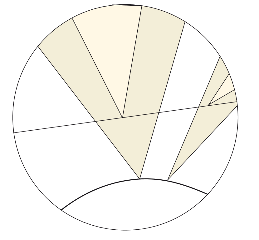
(b) Controlled chords

Figure 7. Controlled and squeezed chords

5.2.2. Squeezing nested pair of chords

In all the sequel $\boldsymbol{K}$ is the diffusion constant defined in Proposition 3.4.6 and $\boldsymbol{\kappa}=\boldsymbol{K}^{-1}$ the contraction constant

The following proposition provides our first example of nested pairs of chords in the coplanar situation.

Proposition 5.2.1.

[Nested pair of chords] There exists $\beta_{1}$ only depending on ${\mathsf{G}}$, and a decreasing function

$$\ell:]0,\beta_{1}]\to\mathbb{R},$$

such that for any positive numbers $\beta$ with $\beta\leqslant\beta_{1}$, any nested pair $(H_{0},H_{1})$ with $\delta(H_{0},H_{1})\geqslant\ell(\beta)$ is $(\boldsymbol{K}\beta,\boldsymbol{\kappa}^{9})$-squeezed. The projection $\tau_{0}$ of $H_{1}$ on $H_{0}$ is a commanding tripod of $(H_{0},H_{1})$

Observe in particular that $S_{0}(H_{1})\subset S_{\boldsymbol{K}\beta}(H_{1})\subset C_{\boldsymbol{\kappa}^{8}\beta}(\tau_{0})$. The choice of $\boldsymbol{\kappa}^{9}$ is rather arbitrary in this proposition but will make our life easier later on.

Proof.

Let $\tau_{1}\in H_{1}$. Let then $\check{\tau}_{0}\in H_{0}$, with $\partial^{0}\check{\tau}_{0}=\partial^{0}\tau_{1}$. Let as in paragraph 3.4.4, $s_{0}$, $s_{1}$, $z_{0}$ and $z_{1}$ be constructed from $\check{\tau}_{0}$ and $\tau_{1}$. One notices that $d_{\tau_{1}}(z,z_{1})\leqslant\pi/2$. Then given $\varepsilon$, for $\delta(H_{0},H_{1})$ large enough the second part of Proposition 3.4.6 yields that $(\check{\tau}_{0},\tau_{1})$ is $(\alpha,\varepsilon)$-nested.

Observe now, that for any $\beta$, there exists $\delta_{1}$ so that $\delta(H_{0},H_{1})>\delta_{1}$ yields $d(\tau_{0},\check{\tau}_{0})\leqslant\beta$, where $\tau_{0}$ is the projection of $H_{1}$ on $H_{0}$ Thus, using Proposition 3.4.4 for $\beta$ small enough, we have that the pair of tripods $(\check{\tau}_{0},\tau_{1})$ is $(\alpha,2\cdotp\varepsilon)$-nested. In other words, since $\tau_{0}$ is independent from the choice of $\tau_{1}$, we have proved that the pair of chords $(H_{0},H_{1})$ is $(\alpha,2\cdotp\varepsilon)$-squeezed for $\delta(H_{0},H_{1})$ large enough.

∎

5.2.3. Controlling nested pair of chords

Our second result about coplanar pair of chords is the following

Lemma 5.2.2.

[Controlling diffusion] There exists a positive numbers $\beta_{2}$, with $\beta_{2}\leqslant\beta_{3}$ only depending on ${\mathsf{G}}$, such that given a positive $\beta\leqslant\beta_{2}$, a nested pair $(H_{0},H_{1})$, then $(H_{0},H_{1})$ is $(\xi\beta,\boldsymbol{K})$ controlled for all $\xi\leqslant 1$.

Assume furthermore that $\ell_{0}\geqslant\delta(H_{0},H_{1})$, where $\ell_{0}\geqslant\ell(\beta)$ Then, given $\tau_{1}\in H_{1}$, there exists $H_{2}$ so that

• $(H_{1},H_{2})$ is nested,

• $0<\delta(H_{0},H_{2})\leqslant\ell_{0}$,

• $(\tau_{0},\tau_{1})$ is $(\boldsymbol{\kappa}^{2}\beta,\boldsymbol{K})$-nested, where $\tau_{0}$ is the projection of $H_{2}$ on $H_{0}$.

Let us first prove

Proposition 5.2.3.

There exists $\alpha_{4}$ with the following property. Let $(H_{0},H_{1})$ be two nested chords and $\tau_{0}\in H_{0}$, $\tau_{1}\in H_{1}$ so that for some $\alpha\leqslant\alpha_{4}$, $C_{\alpha}(\tau_{0})\cap C_{\alpha}(\tau_{1})\not=\emptyset$.

Then $(\tau_{0},\tau_{1})$ are $(\alpha,\boldsymbol{K})$-nested.

Proof.

Observe first that if $(z_{0},\tau_{0},\tau_{1},z_{1})$ are aligned then in that context $d_{\tau_{1}}(\partial^{0}\tau_{1},z_{1})\leqslant\pi/2$ – see figure (8) –.

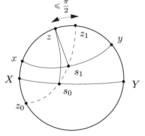
Figure 8. Aligned points and angle

Then Let $u,v\in C_{\alpha}(\tau_{1})$ and $w\in C_{\alpha}(\tau_{0})\cap C_{\alpha}(\tau_{1})$ then by Proposition 3.4.6.

$$d_{\tau_{0}}(u,v) \leqslant \frac{\boldsymbol{K}}{4}d_{\tau_{1}}(u,v)\ ,$$ (25)

$$d_{\tau_{0}}(u,\partial^{0}\tau_{0})\leqslant d_{\tau_{0}}(u,w)+d_{\tau_{0}}(w,\partial^{0}\tau_{0}) \leqslant \frac{\boldsymbol{K}}{4}d_{\tau_{1}}(u,w)+\alpha\leqslant\boldsymbol{K}\alpha\ .$$ (26)

Thus from the second equation $C_{\alpha}(\tau_{1})\leqslant C_{\boldsymbol{K}\alpha}(\tau_{1})$. This concludes the proof of the proposition ∎

Let us now move to the proof of Lemma5.2.2:

Proof.

Let $\tau_{1}\in H_{1}$. Let ${\bf H}^{2}$ be the associated hyperbolic plane to the coplanar pair $(H_{0},H_{1})$. Let $\tau_{0}\in H_{0}$ so that $\partial^{0}\tau_{0}=\partial^{0}\tau_{1}$. Then $\partial^{0}\tau^{0}\in C_{\xi\beta}(\tau_{1})\cap C_{\xi\beta}(\tau_{0})\not=\emptyset$. We conclude proof of the first assertion by Proposition 5.2.3: that $(\tau_{0},\tau_{1})$ is $(\xi\beta,\boldsymbol{K})$-nested.

Assume now that $\delta(H_{0},H_{1})\leqslant\ell_{0}$. Let $H_{3}$ so that $S_{0}(H_{3})=C_{\boldsymbol{\kappa}^{2}\beta}(\tau_{1})\cap\partial_{\infty}{\bf H}^{2}$. We have two cases.

(1)   If $\delta(H_{0},H_{3})\leqslant\ell_{0}$, we can take $H_{2}=H_{3}$, and $\tau_{0}$ the projection of $H_{2}$ on $H_{0}$. Thus $\partial^{0}\tau^{0}\in C_{\boldsymbol{\kappa}^{2}\beta}(\tau_{1})\cap C_{\boldsymbol{\kappa}^{2}\beta}(\tau_{0})\not=\emptyset$ and we conclude by Proposition 5.2.3: $(\tau_{0},\tau_{1})$ is $(\boldsymbol{\kappa}^{2}\beta,\boldsymbol{K})$-nested. (2)   If $\delta(H_{0},H_{3})\geqslant\ell_{0}\geqslant\ell(\beta)$, a continuity argument shows the existence of $H_{2}$ such that the pairs $(H_{1},H_{2})$ and $(H_{2},H_{3})$ are nested and $\delta(H_{0},H_{2})=\ell_{0}$. Let $\tau_{0}$ be the projection of $H_{2}$ on $H_{0}$. Then we have,

$$\left(C_{\boldsymbol{\kappa}^{2}\beta}(\tau_{1})\cap{\bf H}^{2}\right)=S_{0}(H_{3})\subset S_{0}(H_{2})\subset\left(C_{\boldsymbol{\kappa}^{8}\beta}(\tau_{0})\cap{\bf H}^{2}\right)\subset\left(C_{\boldsymbol{\kappa}^{2}\beta}(\tau_{0})\cap{\bf H}^{2}\right)\ ,$$

where the first inclusion follows from the definition of $H_{3}$, the second by the fact of $(H_{2},H_{3})$ is nested, and the previous to last one by Proposition 5.2.1 since $\delta(H_{0},H_{2})\geqslant\ell(\beta)$. In particular $C_{\boldsymbol{\kappa}^{2}\beta}(\tau_{1})\cap C_{\boldsymbol{\kappa}^{2}\beta}(\tau_{0})\not=\emptyset$. Again we conclude by Proposition 5.2.3 : $(\tau_{0},\tau_{1})$ is $(\boldsymbol{\kappa}^{2}\beta,\boldsymbol{K})$-nested.

∎

6. The Confinement Lemma

The main results of this section are the Confinement Lemma and the Weak Confinement Lemma that guarantee that a deformed path of quasi-tripods is squeezed or controlled, provided that the deformation is small enough.

Let us say a coplanar path of tripods associated to a path of chords $(h_{i})_{0\leqslant i\leqslant N}$ is a weak $(\ell,N)$-coplanar path of tripods if

$$\delta(h_{0},h_{i}) \leqslant \ell,\hbox{ for }i<N.$$ (27)

A coplanar path of tripods associated to a sequence of chords $(h_{i})_{0\leqslant i\leqslant N}$ is a strong $(\ell,N)$-coplanar path of tripods if furthermore

$$\delta(h_{0},h_{N}) \geqslant \ell.$$ (28)

.

The main result of this section is the following,

Lemma 6.0.1.

[confinement] There exists $\beta_{3}$ only depending on ${\mathsf{G}}$, such that for every $\alpha$ with $\alpha\leqslant\beta_{3}$ then there exists $\ell_{0}(\alpha)$, so that for all $\ell_{0}\geqslant\ell_{0}(\alpha)$, there is $\eta_{0}$, so that for all $N$

• for all weak $(\ell_{0},N)$-coplanar paths of tripods $\underline{\tau}=(\tau_{0},\ldots,\tau_{N})$, associated to a path of chords $\underline{h}(N)=(h_{0},\ldots,h_{N}),$

• for all $\varepsilon/N$-deformation $v=\left(g_{0},\ldots,g_{N-1}\right)$ with $\varepsilon\leqslant\eta_{0}$

The following holds:

1. the pair $(h_{0}^{v},h_{N}^{v})$ is $(\boldsymbol{\kappa}^{2}\alpha,\boldsymbol{K}^{2})$-controlled,

2. if furthermore $\underline{h}$ is a strong coplanar path of tripods then $(h_{0}^{v},h_{N}^{v})$ is $(\alpha,\boldsymbol{\kappa}^{7})$-squeezed. Moreover $(h_{0}^{v},h_{N}^{v})$ and $(h_{0},h_{N})$ both have the same commanding tripod.

3. If finally, $\underline{h}$ is a strong coplanar path with $\delta(h_{0},h_{N})=\ell_{0}$, then $\check{\tau}_{0}$, the projection of $h_{N}$ on $h_{0}$, is a commanding tripod of $(h_{0}^{v},h_{N}^{v})$.

In the sequel, we shall refer the first case as the Weak Confinement Lemma and the second case as the Strong Confinement Lemma.

6.0.1. Controlling deformations from a tripod

We first prove a proposition that allows us to control the size of deformation from a tripod depending only on the last and first chords.

Proposition 6.0.2.

[Barrier] For any positive $\ell_{0}$, there exists positive constants $k$ and $\eta_{1}$ so that for all integer $N$

• for all weak $(\ell_{0},N)$-coplanar paths of tripods $\underline{\tau}=(\tau_{0},\ldots,\tau_{N})$, associated to a path of chords $\underline{h}(N)=(h_{0},\ldots,h_{N}),$

• for all chord $H$ so that $(h_{N},H)$ is nested with $0<\delta(h_{0},H)\leqslant\ell_{0}$,

• for all $\frac{\varepsilon}{N}$-deformation $v=\left(g_{0},\ldots,g_{N-1}\right)$ with $\varepsilon\leqslant\eta_{1}$,

we have

$$\,\,d_{\check{\tau}_{0}}(\operatorname{Id},b_{N}) \leqslant k\cdotp\varepsilon,$$ (29)

where $b_{N}=g_{0}\cdots g_{N-1}$ and $\check{\tau}_{0}$ is the projection of $H$ on $h_{0}$.

In this proposition, the position of $h_{N}$ plays no role.

6.0.2. The confinement control

We shall use in the sequel the following proposition.

Proposition 6.0.3.

[Confinement control] There exists a positive $\varepsilon_{0}$ so that for every positive $\ell_{0}$, there exists a constant $k$ with the following property;

• Let $(H,h)$ be a pair of nested chords, associated to the circle $C\subset{\bf F}$, so that $0<\delta(h,H)\leqslant\ell_{0}$ and let $\tau_{0}$ be the projection of $h$ on $H$.

• Let $(X,Y)$ and $(x,y)$ be the extremities of $H$ and $h$ respectively.

• Let $u,v,w\in C\subset{\bf F}$ be pairwise distinct so that $(X,u,v,x,y,w,Y)$ is cyclically oriented –possibly with repetition – in $C$ and $\tau$ be the tripod coplanar to $H$ so that $\partial\tau=(u,w,v)$

• Let $g\in\mathsf{P}_{w}$ with $d_{\tau}(g,\operatorname{Id})\leqslant\varepsilon_{0}\ .$

Then

$$d_{\tau_{0}}(g,\operatorname{Id})\leqslant k\cdotp d_{\tau}(g,\operatorname{Id}).$$

Figure (9) illustrates the configuration of this proposition.

Figure 9. Confinement control

Proof.

It is no restriction to assume that $\delta(h,H)=\ell_{0}$. Let $\tau$ and $\tau_{0}$ be as in the statement and $\tau_{1}$ be the tripod coplanar to $H$, so that $\partial\tau_{1}=(u,w,z)$. Observe that, there is a positive $t$ so that $\varphi_{t}(\tau)=\tau_{1}$. Let $a=\mathsf{T}\tau(a_{0})\in\mathfrak{g}$, we have

$$d_{\varphi_{t}(\tau)}(g,\operatorname{Id})=d_{\exp(ta)(\tau)}(g,\operatorname{Id})=d_{\tau}(\exp(-ta)g\exp(ta),\operatorname{Id})\ .$$

Let $\mathfrak{p}_{+}$ be the Lie algebra of $\mathsf{P}_{+}\coloneqq\mathsf{P}_{\partial^{+}\tau}=P_{w}$, that we consider also equipped with the Euclidean norm $\|.\|_{\tau}$. By construction $\mathsf{P}_{+}=\tau(\mathsf{P}^{+}_{0})$, thus

$$\sup_{t>0}\left.\left\|\operatorname{ad}(\exp(-ta))\right\|\right|_{\mathfrak{p}_{+}}<\infty.$$

For $\varepsilon$ small enough and independent of $\partial^{+}\tau$, $\exp$ is $k_{1}$-bilipschitz from the ball of radius $\varepsilon$ in $\mathfrak{p}_{+}$ onto its image in $\mathsf{P}_{+}$ for some constant $k_{1}$ independent of $\partial^{+}\tau$. Thus for $\varepsilon_{0}$-small enough, there exists a constant $k_{1}$ so that

$$d_{\tau_{1}}(g,\operatorname{Id})\leqslant k_{1}d_{\tau}(g,\operatorname{Id}).$$ (30)

Now the set $K$ of tripods $\sigma$ coplanar to $\tau_{0}$, with $\partial\sigma=(u,w,z)$ with $z$ fixed, $u$, $w$ as above, is compact In particular there exists $k_{2}$ only depending on $\ell_{0}$ so that for any tripod $\sigma$ in $K$,

$$d(\tau_{1},\tau_{0})\leqslant k_{3}.$$

Thus by Proposition 3.4.4, there exists $k_{4}$ so that

$$d_{\tau_{1}}(g,\operatorname{Id})\leqslant k_{4}\cdotp d_{\sigma}(g,\operatorname{Id}).$$

The proposition now follows by combining with inequality (30). ∎

6.0.3. Proof of the Barrier Proposition 6.0.2

Let $(x_{i},x^{i})$ be the extremities of $h_{i}$ where $x_{i}$ is the pivot. Let $\widehat{x}_{i+1}$ the vertex of $\tau_{i}$ different from $x_{i}$ and $x^{i}$.

Let $\check{\tau}_{0}$ be the projection of $H$ on $h_{0}$. Observe that $x_{i}$ lies in one of the connected component of $h_{0}\setminus H$, while $x^{i}$ and lie in the other (see Figure (10)).

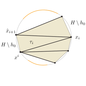
Figure 10.

Thus, according to Proposition 6.0.3 for $\varepsilon$ small enough there exists $k$, only depending on $\ell$ so that

$$d_{\tau_{0}}(g_{i},\operatorname{Id})\leqslant k\cdotp d_{\tau_{i}}(g_{i},\operatorname{Id})\leqslant k\cdotp\frac{\varepsilon}{N}.$$

Thus, using the right invariance of $d_{\tau_{0}}$,

$$d_{\tau_{0}}\left(\operatorname{Id},b_{N}\right)\leqslant\sum_{i=1}^{N}d_{\tau_{0}}\left(\Pi_{j=i}^{N}g_{j},\Pi_{j=i+1}^{N}g_{j}\right)=\sum_{i=1}^{N}d_{\tau_{0}}\left(g_{i},\operatorname{Id}\right)\leqslant k\cdotp\varepsilon.$$

Observe that this proves inequality (29) and concludes the proof of the Barrier Proposition 6.0.2.

6.0.4. Proof of the Confinement Lemma 6.0.1

Let $\beta_{1}$ as in Proposition 5.2.1. Let then $\alpha$ with $\alpha\leqslant\beta_{1}$. According to Proposition 5.2.1, there exists $\ell=\ell_{0}(\alpha)$ so that if $(H_{0},H_{1})$ is a nested pair of chords with $\delta(H_{0},H_{1})\geqslant\ell$, then for any $\sigma_{1}\in H_{1}$, the pair $(\tau_{0},\sigma_{1})$ is $(\boldsymbol{K}\alpha,\boldsymbol{\kappa}^{9})$-nested, where $\tau_{0}$ is the projection of $H_{1}$ on $H_{0}$. Let now fix $\ell_{0}\geqslant\ell_{0}(\alpha)$

First step: strong coplanar

Consider first the case where $\delta(h_{0},h_{N})\geqslant\ell_{0}$. By continuity we may find a chord $\check{h}_{N}$ so that the pairs $(h_{N-1},\check{h}_{N})$ and $(\check{h}_{N},h_{N})$ are nested and so that $\delta(\check{h}_{N},h_{0})=\ell_{0}$.

Let $\check{\tau}_{0}$ be the projection of $\check{h}_{N}$ on $h_{0}$. Then by Proposition 5.2.1 for any $\sigma_{1}$ in $\check{h}_{N}$, $(\check{\tau}_{0},\sigma_{1})$ is $(\boldsymbol{K}\alpha,\boldsymbol{\kappa}^{9})$-nested

By Lemma 5.2.2, for any $\sigma_{N}$ in $h_{N}$, there exist $\sigma_{1}$ in $\check{h}_{N}$ so that $(\sigma_{1},\sigma_{N})$ is $(\alpha,\boldsymbol{K})$-nested and thus $(\check{\tau}_{0},\sigma_{N})$ is $(\alpha,\boldsymbol{\kappa}^{8})$-nested.

By the Barrier Proposition 6.0.2 applied to $\underline{h}(N)$ and $H=\check{h}_{N},$ we get that

$$d_{\check{\tau}_{0}}(\operatorname{Id},b_{N})\leqslant k\cdotp\varepsilon\,.$$

for $k$ only depending on ${\mathsf{G}}$ and where $\ell$ and $b_{N}$ are defined in the Barrier Proposition.

We now furthermore assume that $\alpha\leqslant\beta_{0}$, where $\beta_{0}$ comes from Proposition 5.1.4. For $\varepsilon$ is small enough, Proposition 5.1.4 shows that for any $\sigma_{1}$ in $h_{N}$; $(\check{\tau}_{0},b_{N}(\sigma_{1}))$ is $(\alpha,2\boldsymbol{\kappa}^{8})$-nested. Thus $(h_{0},b_{N}(h_{N}))$ is $(\alpha,2\boldsymbol{\kappa}^{8})$-squeezed hence $(\alpha,\boldsymbol{\kappa}^{7})$-since $2\boldsymbol{\kappa}\leqslant 1$, with $\check{\tau}_{0}$ as a commanding tripod.

This applies of course if the deformation is trivial and we see that $(h_{0},h_{N})$ and $(h_{0}^{v},h_{N}^{v})$ both have $\check{\tau}_{0}$ as a commanding tripod.

This concludes this first step and the proof of the second item and the third item in Lemma 6.0.1.

Second step

Let us consider the remaining case when $\delta(h_{0},h_{N})\leqslant\ell$. Let us apply Proposition 5.2.2 to $(H_{0},H_{1})=(h_{0},h_{N})$ and $\tau_{1}$ in $h_{N}$. Thus there exists $H_{2}$ so that $(h_{N},H_{2})$ is nested, $0<\delta(H_{0},H_{2})\leqslant\ell$, and $(\tau_{0},\tau_{1})$ is $(\boldsymbol{\kappa}^{2}\alpha,\boldsymbol{K})$ nested where $\tau_{0}$ is the projection of $H_{2}$ on $h_{0}$.

Applying the Barrier Proposition 6.0.2 to $h=H_{2}$ and $H=H_{0}$, yields that $d_{\tau_{0}}(\operatorname{Id},b_{N})\leqslant k\cdotp\varepsilon$. Thus for $\varepsilon$ small enough, then Proposition 5.1.4 yields that $(\tau_{0},b_{N}(\tau_{1})$ is $(\boldsymbol{\kappa}^{2}\alpha,2\boldsymbol{K})$ nested, hence $(\boldsymbol{\kappa}^{2}\alpha,\boldsymbol{K}^{2})$ nested.

This shows that $(h_{0},b_{N}(h_{N}))$ is $(\boldsymbol{\kappa}^{2}\alpha,\boldsymbol{K}^{2})$-controlled. This concludes the proof of Lemma 6.0.1.

7. Infinite paths of quasi-tripods and their limit points

The goal of this section is to make sense of the limit point of an infinite sequence of quasi-tripods and to give a condition under which such a limit point exists. The ad hoc definitions are motivated by the last section of this paper as well as by the discussion of Sullivan maps.

One mays think of our main Theorem 7.2.1 as a refined version of a Morse Lemma in higher rank: instead of working with quasi-geodesic paths in the symmetric space, we work with sequence of quasi-tripods in the flag manifold; instead of making the quasi-geodesic converge to a point at infinity, we make the sequence of quasi-tripods shrink to a point in the flag manifold. This is guaranteed by some local conditions that will allow us to use our nesting and squeezing concepts defined in the preceding section.

Theorem 7.2.1 is the goal of our efforts in this first part and will be used several times in the future.

7.1. Definitions: $Q$-sequences and their deformations

Definition 7.1.1.

1. A $Q$ coplanar sequence of tripods is an infinite sequence of tripods $\underline{T}=\{{T}_{m}\}_{m\in\mathbb{N}}$ so that the associated sequence of coplanar chords $\underline{c}=\{c_{i}\}_{i\in\mathbb{N}}$ satisfies: for all integers $m$ and $p$ we have

   $$|m-p|\leqslant Q\delta(c_{m},c_{p})+Q$$

   where $\delta(\cdot,\cdot)$ is the shift defined in 5.2.1.

2. A sequence of quasi-tripod $\underline{\tau}=\{{\tau}_{m}\}_{m\in\mathbb{N}}$ is a $(Q,\varepsilon)$-sequence of quasi-tripods if there exists a a coplanar $Q$ coplanar sequence of tripods $T=\{{T}_{m}\}_{m\in\mathbb{N}}$, so that for every $n$, $\{\tau_{m}\}_{m\in[0,n]}$ is an $\varepsilon$-deformation of $\{T_{m}\}_{m\in[0,n]}$.

3. The associated sequence of chords to a $(Q,\varepsilon)$-sequence of quasi-tripods is called a $(Q,\varepsilon)$-sequence of chords

7.2. Main result: existence of a limit point

Our main theorem asserts the existence of limit points for some deformed $(Q,\varepsilon)$- sequence and their quantitative properties.

Theorem 7.2.1.

[Limit point] There exist some positive constants ${\rm A}$ and ${\rm q}$ only depending on ${\mathsf{G}}$, with ${\rm q}<1$, such that for every positive number $\beta$ and $\ell_{0}$ with $\beta\leqslant{\rm A}$, there exist a positive constant $\varepsilon>0$, so that for any $R>1$:

For any $(\ell_{0}R,\frac{\varepsilon}{R})$-deformed sequence of quasi tripods $\underline{\theta}=\{{\theta}_{m}\}_{m\in\mathbb{N}}$, with associated sequence of chords $\underline{\Gamma}=\{{\Gamma}_{m}\}_{m\in\mathbb{N}}$ there exists some $\delta>0$ so that

$$\bigcap_{m}^{\infty}S_{\delta}(\Gamma_{m}):=\{\xi(\underline{\theta})\}\ ,\hbox{ with }\xi(\underline{\theta})=\lim_{m\to\infty}(\partial^{j}\theta_{m})\ \ \hbox{ for }j\in\{+,-,0\}\ ,$$ (31)

moreover we have the following quantitative estimates:

1. for any $\tau$ in $\Gamma_{0}$, and $m>(\ell_{0}+1)^{2}R$,

   $$d_{\tau}(\xi(\underline{\theta}),\partial^{j}\theta_{m}))\leqslant{\rm q}^{m}\beta\ \ \hbox{ for }j\in\{+,-,0\}\ .$$ (32)

2. Let $\tau$ in $\Gamma_{0}$. Assume $\{{\theta}_{m}\}_{m\in\mathbb{N}}$ is the deformation of a sequence of coplanar tripods $\underline{\tau}=\{{\tau}_{m}\}_{m\in\mathbb{N}}$ with $\tau_{0}=\accentset{\mbox{\large.}}{\theta_{0}}$, then

   $$d_{\tau}(\xi(\underline{\theta}),\xi(\underline{\tau}))\leqslant\beta\,.$$ (33)

3. Finally, let $\{{\theta^{\prime}}_{m}\}_{m\in\mathbb{N}}$ be another $(\ell_{0}R,\frac{\varepsilon}{R})$-deformed sequence of quasi tripods. Assume that $\{{\theta^{\prime}}_{m}\}_{m\in\mathbb{N}}$ and $\{{\theta}_{m}\}_{m\in\mathbb{N}}$ coincides up to the $n$-th chord with $n>(\ell_{0}+1)^{2}R$, then for all $\tau\in\Gamma_{0}$,

   $$d_{\tau}(\xi(\underline{\theta^{\prime}}),\xi(\underline{\theta}))\leqslant{\rm q}^{n}\beta\ .$$ (34)

The limit point theorem will be the consequence of a more technical one:

Theorem 7.2.2.

[Squeezing chords] There exists some constant ${\rm A}$, only depending on ${\mathsf{G}}$, such that for every positive number $\delta$ with $\delta\leqslant{\rm A}$, there exists positive constants $R_{0}$, $\ell_{0}$ and $\varepsilon$ with the following property:

If $\underline{\Gamma}$ is an $(\ell_{0}R,\frac{\varepsilon}{R})$-deformed sequence of chords of the coplanar sequence of chords $\underline{c}$ with $R\geqslant R_{0}$, if $j>i$ are so that $\delta(c_{i},c_{j})\geqslant\ell_{0}$ then $(\Gamma_{i},\Gamma_{j})$ is $(\delta,\boldsymbol{\kappa})$-squeezed.

7.3. Proof of the squeezing chords theorem 7.2.2

As a preliminary, we make the choice of constants, then we cut a sequence of chords into small more manageable pieces. Finally we use the Confinement Lemma to obtain the proof.

7.3.1. Fixing constants and choosing a threshold

Let $\alpha_{3}$ as in Corollary 5.1.3, let $\beta_{3}$ as in the Confinement Lemma 6.0.1. We now choose $\alpha$ so that

$$\alpha\leqslant\inf(\beta_{3},\alpha_{3}).$$ (35)

Then $\ell_{0}=\ell_{0}(\alpha)$ be the threshold, and $\eta_{0}$ be obtained by the Confinement Lemma 6.0.1. Let finally

$$\varepsilon\leqslant\frac{\eta_{0}}{\ell_{0}\cdotp(\ell_{0}+1)}\ .$$ (36)

7.3.2. Cutting into pieces

Let $\underline{c}$ be a sequence of coplanar chords admitting an $\ell_{0}R$-coplanar path of tripods.

Lemma 7.3.1.

We can cut $\underline{\tau}$ into successive pieces $\underline{\tau}^{n}:=\{\tau_{p}\}_{p_{n}\leqslant p<p_{n+1}}$ for $n\in\{0,M\}$ so that

1. for $n\in\{0,M-1\}$, $\underline{\tau}^{n}$ is a strong $(\ell_{0},N)$ coplanar path of tripods

2. $\underline{\tau}^{M}$ is a weak $(\ell_{0},N)$ coplanar path of tripods.

where in both cases, $N\leqslant L\coloneqq\lfloor(\ell_{0}+1)(\ell_{0}R)\rfloor+1$, where $\lfloor x\rfloor$ denotes the integer value of the real number $x$.

Proof.

Let $\underline{c}$ be the corresponding sequence of chords. Recall that the function $q\mapsto\delta(c_{p},c_{q})$ is increasing for $q>p$. Thus we can further cut into (maximal) pieces so that

$$\delta(c_{p_{n}},c_{p_{n+1}-1}))\leqslant\ell_{0},\ \ \delta(c_{p_{n}},c_{p_{n+1}}))\geqslant\ell_{0}.$$

This gives the lemma: the bound on $N$ comes from the fact that $\underline{\tau}$ is a $\ell_{0}R$-sequence. In particular, since $\delta(c_{p_{n}},c_{p_{n+1}-1})\leqslant\ell_{0}$, then $|p_{n+1}-p_{n}|-1\leqslant(\ell_{0}R)(\ell_{0}+1)$.∎

7.3.3. Completing the proof

Let $\underline{\theta}$ be an $(\ell_{0}R,\frac{\varepsilon}{R})$-sequence of quasi-tripods, with $R>R_{0}$. Let $\underline{\Gamma}$ be the associated sequence of chords. Assume $\underline{\theta}$ is the deformation of an $\ell_{0}R$- coplanar sequence of tripods $\underline{\tau}$, cut in smaller sub-pieces as in Lemma 7.3.1.

Proposition 7.3.2.

for all $n$

1. for $n<M$, $(\Gamma_{p_{n}},\Gamma_{p_{n+1}})$ is $(\alpha,\boldsymbol{\kappa}^{7})$-squeezed,

2. Moreover $(\Gamma_{p_{M}},\Gamma_{p_{M+1}})$ is $(\boldsymbol{\kappa}^{2}\alpha,\boldsymbol{K}^{2})$-controlled.

Proof.

If $n<M$, $\underline{\tau^{n}}$ is a strong $(\ell_{0},L)$-path. Then according to the Confinement Lemma 6.0.1 and the choice of our constants $(\Gamma_{p_{n}},\Gamma_{p_{n+1}})$ is $(\alpha,\boldsymbol{\kappa}^{7})$-squeezed.

Since $\underline{\tau}^{M}$ is a weak $(\ell_{0},L)$-path, it follows by our choice of constants and the Confinement Lemma 6.0.1 that $(\Gamma_{p_{M}},\Gamma_{p_{M+1}})$ is $(\boldsymbol{\kappa}^{2}\alpha,\boldsymbol{K}^{2})$ controlled.∎

We now prove the Squeezing Chord Theorem 7.2.2 with $\delta=\boldsymbol{\kappa}^{2}\alpha$:

Proposition 7.3.3.

Assuming, $\delta(c_{i},c_{j})>\ell_{0}$ and $j>i$, the pair $(\Gamma_{i},\Gamma_{j})$ is $(\boldsymbol{\kappa}^{2}\alpha,\boldsymbol{\kappa})$-squeezed.

Proof.

We will use freely the observation that $(\alpha,\boldsymbol{\kappa}^{n})$-nesting implies $(\boldsymbol{\kappa}^{p}\alpha,\boldsymbol{\kappa}^{q})$-nesting for $p,q\geqslant 0$ with $p+q\leqslant n$.

Recall that thanks to the Composition Proposition 5.1.2, if the pairs of chords $(H_{0},H_{1})$ and $(H_{1},H_{2})$ which are both $(\alpha,\boldsymbol{\kappa}^{7})$-squeezed. (in particular $(H_{1},H_{2})$ is $(\alpha,\boldsymbol{\kappa}^{5})$-squeezed), then $(H_{0},H_{2})$ is $(\alpha,\boldsymbol{\kappa}^{7})$-squeezed.

We cut $\underline{\tau}$ as above in pieces and control every sub-piece using Proposition 7.3.2.

Thus, by induction, $(\Gamma_{p_{0}},\Gamma_{p_{M}})$ is $(\alpha,\boldsymbol{\kappa}^{7})$-squeezed and thus $(\boldsymbol{K}^{2}(\boldsymbol{\kappa}^{2}\alpha),\boldsymbol{\kappa}^{7})$-squeezed since $\boldsymbol{\kappa}\boldsymbol{K}=1$.

Finally since $(\Gamma_{p_{M}},\Gamma_{p_{M+1}})$ is $(\boldsymbol{\kappa}^{2}\alpha,\boldsymbol{K}^{2})$-controlled, the Composition Proposition 5.1.2 yields that $(\Gamma_{p_{0}},\Gamma_{p_{M+1}})$ is $(\boldsymbol{\kappa}^{2}\alpha,\boldsymbol{\kappa}^{7}\boldsymbol{K}^{2})$-squeezed and thus $(\boldsymbol{\kappa}^{2}\alpha,\boldsymbol{\kappa})$-squeezed. This finishes the proof. ∎

7.4. Proof of the existence of limit points, Theorem 7.2.1

Let $\{{\theta}_{m}\}_{m\in\mathbb{N}}$ and $\{{\tau}_{m}\}_{m\in\mathbb{N}}$ be sequences of quasi tripods and tripods as in Theorem 7.2.1.

Let $\underline{\Gamma}$ be the sequence of chords associated to $\{{\theta}_{m}\}_{m\in\mathbb{N}}$ and similarly $\underline{c}$ associated to $\{{\tau}_{m}\}_{m\in\mathbb{N}}$ as in Theorem 7.2.1, then according to Theorem 7.2.2 if $j>i$ are so that if $\delta(c_{i},c_{j})\geqslant\ell_{0}$ then $(\Gamma_{i},\Gamma_{j})$ is $(\delta,\boldsymbol{\kappa})$-squeezed. Since $\underline{c}$ is $Q_{0}$-controlled (with $Q_{0}=\ell_{0}R$) we have

$$\delta(c_{i},c_{j})\geqslant\frac{|i-j|}{\ell_{0}R}-1,$$

Thus

$$j-i\geqslant L\implies\delta(c_{i},c_{j})\geqslant\ell_{0},$$

We can summarize this discussion in the following statement

$$j-i\geqslant L\implies S_{\delta}(\Gamma_{j})\subset S_{\boldsymbol{\kappa}\delta}(\Gamma_{i})\,,$$ (37)

7.4.1. Convergence for lacunary subsequences

We first prove an intermediate result.

Corollary 7.4.1.

There exists a constant ${\rm M}$ only depending on ${\mathsf{G}}$, with ${\rm q}<1$, such that for $\delta$ small enough, if $\underline{l}=\{{l}_{m}\}_{m\in\mathbb{N}}$ is a sequence so that $l_{m+1}\geqslant l_{m}+L$ and $l_{0}=0$, then

$$S_{\delta}(\Gamma_{l_{m+1}})\subset S_{\boldsymbol{\kappa}\delta}(\Gamma_{l_{m}}),$$ (38)

and furthermore there exists a unique point $\xi(\underline{l})\in{\bf F}$ so that

$$\bigcap_{m=1}^{\infty}S_{\delta}\left(\Gamma_{l_{m}}\right)=\left\{\xi(\underline{l})\right\}\subset C_{\delta}(\check{\tau}_{0}).$$ (39)

where $\check{\tau}_{0}$ is a commanding tripod for $(\Gamma_{0},\Gamma_{l_{1}})$.

Finally, if $\tau\in\Gamma_{0}$ then for all $u$ in $S_{\delta}(\Gamma_{l_{m}})$ with $m\geqslant 1$ we have

$$d_{\tau}(u,\xi(\underline{l}))\leqslant 2^{-m}{{\bf M}}\delta.$$ (40)

Proof.

From the squeezed condition for chords, we obtain that there exists $\check{\tau}_{m}\in\Gamma_{l_{m}}$ so that

$$S_{\delta}(\Gamma_{l_{m+1}})\subset C_{\boldsymbol{\kappa}\delta}(\check{\tau}_{m})\subset S_{\boldsymbol{\kappa}\delta}(\Gamma_{l_{m}}).$$

This proves the first assertion. As a consequence, $C_{\delta}(\check{\tau}_{m+1})\subset C_{\boldsymbol{\kappa}\delta}(\check{\tau}_{m})$. Combining with the Convergence Corollary 5.1.3, we get the second assertion, with

$$\{\xi(\underline{l})\}:=\bigcap_{m=1}^{\infty}C_{\delta}(\check{\tau}_{m})=\bigcap_{m=1}^{\infty}S_{\delta}(\check{\tau}_{m})$$

Using the second assertion of the Convergence Corollary 5.1.3, we obtain that if $u,v\in S_{\delta}(\Gamma_{l_{m}})\subset C_{\delta}(\check{\tau}_{m-1})$, then

$$d_{\tau_{0}}(u,v)\leqslant 2^{2-m}\delta.$$

and in particular $u,\xi(\underline{l})\in C_{\delta}(\check{\tau}_{0})$ and

$$d_{\tau_{0}}(u,\xi(\underline{l}))\leqslant 2^{2-m}\delta.$$ (41)

We now extend the previous inequality when we replace $\tau_{0}$ by any $\tau\in C_{n}$. We use Lemma 5.1.5 which produces constant $\delta_{0}$ and $k$ only depending on ${\mathsf{G}}$ so that if $\delta$ is smaller than $\delta_{0}$ then since $u,\xi(\underline{l})\in C_{\delta}(\check{\tau}_{0})$,

$$d_{\tau}(u,\xi(\underline{l}))\leqslant k.d_{\tau_{0}}(u,\xi(\underline{l})).$$ (42)

This concludes the proof of the corollary since we now get from inequalities (42) and (41)

$$d_{\tau}(u,\xi(\underline{l}))\leqslant k.2^{2-m}\delta.$$

∎

7.4.2. Completion of the proof

Let $\{{l}_{m}\}_{m\in\mathbb{N}}$ and $\{{l^{\prime}}_{m}\}_{m\in\mathbb{N}}$ be two subsequences. It follows from inclusion (37), that

$$\bigcap_{m=1}^{\infty}S_{\delta}\left(\Gamma_{l_{m}}\right)=\bigcap_{m=1}^{\infty}S_{\delta}\left(\Gamma_{l^{\prime}_{m}}\right).$$

As an immediate consequence, we get that

$$\bigcap_{m=1}^{\infty}S_{\delta}\left(\Gamma_{m}\right)=\left\{\xi\left(\underline{\lambda}\right)\right\},$$

where $\underline{\lambda}=\{{\lambda}_{m}\}_{m\in\mathbb{N}}$, with $\lambda_{m}=m.L$. Thus we may write $\xi\left(\underline{\lambda}\right)\eqqcolon\xi\left(\underline{\Gamma}\right)$. The existence of $\xi(\underline{c})$ follows form the fact that $\underline{c}$ is also a $(\ell_{0}R,\frac{\varepsilon}{R})$-deformed sequence of cuffs.

By construction – and see the second item in the Confinement Lemma 6.0.1 – the commanding tripod $\check{\tau}_{0}$ of $(\Gamma_{0},\Gamma_{L})$ is the commanding tripod of $(c_{0},c_{L})$.

It follows that both $\xi(\underline{l})$ and $\xi(\underline{\lambda})$ belong to $C_{\delta}(\check{\tau}_{0})$. Thus using the triangle inequality and Lemma 5.1.5, for all $\tau\in\Gamma_{0}$,

$$d_{\tau}(\xi(\underline{l}),\xi(\underline{\lambda}))\leqslant k\delta\ ,$$ (43)

where $k$ only depends on $\mathsf{G}$. By inequality (40), if $\{{l}_{m}\}_{m\in\mathbb{N}}$ is a lacunary subsequence, for any $\tau\in\gamma_{0}$, for $u\in S_{\delta}(\Gamma_{l_{m}})$ with $m\geqslant 1$,

$$d_{\tau}(\xi(\underline{\lambda}),u)\leqslant 2^{-m}{{\bf M}}\delta\ .$$ (44)

In particular taking $l_{m}=mL$, one gets

$$d_{\tau}(\xi(\underline{\lambda}),\theta^{j}_{m.L})\leqslant 2^{-m}{{\bf M}}\delta.$$ (45)

Let now $n=(m+1)L+p$, with $p\in[0,L]$. The inclusion (37), gives the first inclusion below, whereas the second is a consequence of the fact that $\boldsymbol{\kappa}<1$

$$S_{\delta}(\Gamma_{n})\subset S_{\boldsymbol{\kappa}\delta}(\Gamma_{m.L})\subset S_{\boldsymbol{\kappa}\delta}(\Gamma_{m.L})\ .$$ (46)

Thus combining the previous assertion with assertion (44) for all $u\in S_{\delta}(\Gamma_{n})$, with $n>L$ we have

$$d_{\tau}(\xi(\underline{\lambda}),u)\leqslant 2^{-m}{{\bf M}}\delta\leqslant(2^{-\frac{1}{L}})^{n}4{{\bf M}}\delta\ .$$ (47)

Taking ${\rm q}=2^{-\frac{1}{L}}$ and $\beta=4{{\bf M}}\delta$, and $u=\theta^{j}_{n}$ yields the inequality

$$d_{\tau}(\xi(\underline{\lambda}),\theta^{j}_{n})\leqslant{\rm q}^{n}\beta\ .$$ (48)

This completes the proof of inequality (32) for $n>L$.

The second item comes from inequality (43) after possibly changing $\beta$.

The third item comes form the first and the triangle inequality, again after changing $\beta$.

8. Sullivan limit curves

The purpose of this section is to define and describe some properties of an analog of the Kleinian property: being a $K$-quasi-circle with $K$ close to 1.

This is achieved in Definition 8.1.1. We then show, under the hypothesis of a compact centralizer for the $\mathfrak{sl}_{2}$, three main theorems of independent interest: Sullivan maps are Hölder (Theorem 8.1.2), a representation with a Sullivan limit map is Anosov (Theorem 8.1.3), and finally one can weaken the notion of being Sullivan under some circumstances (Theorem 8.5.1).

In this paragraph, as usual, $\mathsf{G}$ will be a semisimple group, $\mathfrak{s}$ an $\mathfrak{sl}_{2}$-triple, ${\bf F}$ the associate flag manifold. We will furthermore assume in this section that

The centralizer of $\mathfrak{s}$ is compact

We will comment on the case of non compact centralizer later.

Let us start with a comment on our earlier definition of circle maps 3.1.4. Let $T=(x^{-},x^{+},x_{0})$ be a triple of pairwise distinct points in ${\bf P}^{1}(\mathbb{R})$ – also known as a tripod for $\mathsf{SL}_{2}(\mathbb{R})$ – and $\tau$ a tripod in $\mathcal{G}$. Such a pair $(T,\tau)$ defines uniquely

• an associated circle map $\eta$ from ${\bf P}^{1}(\mathbb{R})$ to ${\bf F}$ so that $\eta(T)=\partial\tau$,

• an associated extended circle map which is a map $\nu$ from the space of triples of pairwise distinct points $(x,y,z)$ in ${\bf P}^{1}(\mathbb{R})$ to $\mathcal{G}$ whose image consists of coplanar tripods and so that

  $$\partial\nu(x,y,z)=(\eta(x),\eta(y),\eta(z))\ ,\ \ \ \nu(x^{-},x^{+},x_{0})=\tau\ .$$

8.1. Sullivan curves: definition and main results

Definition 8.1.1.

[Sullivan curve] We say a map $\xi$ from ${\bf P^{1}}(\mathbb{R})$ to ${\bf F}$ is a $\zeta$-Sullivan curve with respect to $\mathfrak{s}$ if the following property holds:

Let $T=(x^{-},x^{+},x^{0})$ be any triple of pairwise distinct point in ${\bf P}^{1}(\mathbb{R})$. Then there exists a tripod $\tau$ – called a compatible tripod – a circle map $\eta$, with $\eta(T)=\partial\tau$, so that for all $y\in{\bf P^{1}}(\mathbb{R})$,

$$d_{\tau}(\xi(y),\eta(y)) \leqslant \zeta\,.$$ (49)

Obviously if $\zeta$ is large, for instance greater than $\operatorname{diam}({\bf F})$, the definition is pointless: every map is a $\zeta$-Sullivan. We will however show that the definition makes sense for $\zeta$ small enough.

We also leave to the reader to check that in the case of ${\mathsf{G}}=\mathsf{PSL}_{2}(\mathbb{C})$ – so that ${\bf F}$ is ${\bf P}^{1}(\mathbb{C})$ – the following holds: for $K>1$ and any compact interval $C$ containing $-1$, there exists a positive $\varepsilon$ such that if $\xi$ is $\varepsilon$-Sullivan, then for all $(x,y,z,t)$ in ${\bf P}^{1}(\mathbb{R})$ so that $[x,y,z,t]$ belongs to $C$, then

$$\frac{1}{K}\leqslant\left|\frac{[\xi(x),\xi(y),\xi(z),\xi(t)]}{[x,y,z,t]}\right|\leqslant K.$$

This readily implies that $\xi$ is a quasicircle. Thus in that case, an $\varepsilon$-Sullivan map is quasi-symmetric for $\varepsilon$-small enough. The following results of independent interest justify our interest of $\zeta$-Sullivan maps.

Theorem 8.1.2.

[Hölder property] There exists some positive numbers $\zeta$ and $\alpha$, so that any $\zeta$-Sullivan map is $\alpha$-Hölder.

We prove a more quantitative version of this theorem with an explicit modulus of continuity in paragraph 8.3.This modulus of continuity will be needed in other proofs.

The existence of $\zeta$-Sullivan limit maps implies some strong dynamical properties. We refer to [20, 12] for background and references on Anosov representations.

Theorem 8.1.3.

[Sullivan implies Anosov] There exists some positive $\zeta_{1}$ with the following property. Assume $S$ is a closed hyperbolic surface and $\rho$ a representation of $\pi_{1}(S)$ in ${\mathsf{G}}$. Assume there exists a $\rho$-equivariant $\zeta_{1}$-Sullivan map

$$\xi:\partial_{\infty}\pi_{1}(S)={\bf P}^{1}(\mathbb{R})\to{\bf F}\ .$$

Then $\rho$ is $\mathsf{P}$-Anosov and $\xi$ is its limit curve.

Recall that $\mathsf{P}$ is the stabilizer of a point in ${\bf F}$. We recall that a $\mathsf{P}$-Anosov representation is in particular faithful and a quasi-isometric embedding and that all its elements are loxodromic [20, 12] . Recall also that in that context, the parabolic is isomorphic to its opposite. We prove this theorem in paragraph 8.4.

During the proof we shall also prove the following lemma of independent interest

Lemma 8.1.4.

Let $\rho_{0}$ be an Anosov representation of a Fuchsian group $\Gamma$. Assume that the limit map $\xi_{0}$ is $\zeta$-Sullivan, then, for any positive $\varepsilon$, any nearby (i.e., sufficiently close to $\rho_{0}$) representation $\rho$ is Anosov with a $(\zeta+\varepsilon)$-Sullivan limit map.

The following result is is worth stating, although we will not use it in the proof.

Proposition 8.1.5.

Let $\rho_{n}$ be a family of $\mathsf{P}$-Anosov representations of a Fuchsian group, whose limit maps are $\zeta_{n}$-Sullivan, with $\zeta_{n}$ converging to zero. Then, after conjugation, $\rho_{n}$ converges to a representation whose limit curve is a circle.

Proof.

Let $\xi_{n}$ be the limit curve of $\rho_{n}$. By definition, there exists a tripod $\tau_{n}$ and and associated circle map $\eta_{n}$ so that

$$\eta_{n}(0,1,\infty) = \partial\tau_{n}$$

$$d_{\tau_{n}}(\eta_{n},\xi_{n}) \leqslant \zeta_{n}\ .$$

After conjugating $\rho_{n}$ by an element $g_{n}$, we may assume that $\tau_{n}$ and $\eta_{n}$ are constant equal to $\tau$ and $\eta$ respectively. Thus we have

$$\eta(0,1,\infty) = \partial\tau$$

$$d_{\tau}(\eta,\xi_{n}) \leqslant \zeta_{n}\ .$$

In particular, it follows that $\xi_{n}$ converges uniformly to $\eta$. Let $\rho_{0}$ be the Fuchsian representation associated to $\eta$. Let now $\gamma^{i}$ be generators of $\Gamma$. The same argument as above show that $\xi_{n}\circ\gamma_{i}=\rho_{n}(\gamma^{i})\circ\xi_{n}$ converges to $\eta\circ\gamma_{i}=\rho_{0}(\gamma_{i})$. It follows that, using the fact that the centralizer of a circle is compact, that we may extract a subsequence so that $\rho_{n}(\gamma_{i})$ converges for all $i$ to $\rho(\gamma^{i})$, where $\rho$ is a representation in $\mathsf{H}\times\mathsf{K}$ of the form $(\rho_{0},\rho_{1})$, where $\mathsf{H}$ the group isomorphic to $\mathsf{SL}_{2}(\mathbb{R})$ associated to $\eta$, and $\mathsf{K}$ its centralizer.. ∎

In the first paragraph of this section, we single out the consequence of the “compact stabilizer hypothesis” that we shall use.

8.1.1. The compact stabilizer hypothesis

Our standing hypothesis will have the following consequence

Lemma 8.1.6.

The following holds

1. There exists a positive constant $\boldsymbol{\zeta}$, so that for every positive real number $M$, there exists a positive real number $N$, such that if $\xi$ is a $\boldsymbol{\zeta}$-Sullivan map, if $T_{1}$ and $T_{2}$ are two triples of distinct points in ${\bf P}^{1}(\mathbb{R})$ with $d(T_{1},T_{2})\leqslant M$, if $\tau_{1}$ and $\tau_{2}$ are the respective compatible tripods with respect to $\xi$, then

   $$d(\tau_{1},\tau_{2})\leqslant N.$$

2. For any positive $\varepsilon$ and $M$, then for $\zeta$ small enough, for any $\zeta$-Sullivan map $\xi$, if $T_{1}$ and $T_{2}$ are two triples of distinct points in ${\bf P}^{1}(\mathbb{R})$ with $d(T_{1},T_{2})\leqslant M$, if $\tau_{1},\nu_{1}$ are the compatible tripods and extended circle maps of $T_{1}$ with respect to $\xi$, then we may choose a compatible tripod $\tau_{2}$ for $T_{2}$ so that

   $$d(\tau_{2},\nu_{1}(T_{2}))\leqslant\varepsilon.$$

Actually this lemma will be the unique consequence of our standard hypothesis which will be used in the proof. This lemma is itself a corollary of the following proposition.

Proposition 8.1.7.

1. There exists positive constants $\boldsymbol{A}$ and $\boldsymbol{\zeta}_{0}$, such that if $\tau_{1}$ and $\tau_{2}$ are two tripods and $X$ is a triple of points in ${\bf F}$, we have the implication

   $$d_{\tau_{1}}(X,\partial\tau_{1})\leqslant\boldsymbol{\zeta}_{0},\ \ d_{\tau_{2}}(X,\partial\tau_{2})\leqslant\boldsymbol{\zeta}_{0}\implies d(\tau_{1},\tau_{2})\leqslant\boldsymbol{A}\ .$$

2. Moreover, given $\alpha>0$, there exist $\varepsilon>0$ so that

   $$d_{\tau_{1}}(X,\partial\tau_{1})\leqslant\varepsilon,\ \ d_{\tau_{2}}(X,\partial\tau_{2})\leqslant\varepsilon\implies\exists\tau_{3}\ ,\hbox{ with }\partial\tau_{3}=\partial\tau_{2}\hbox{ and }d(\tau_{1},\tau_{3})\leqslant\alpha\ .$$

We first prove Lemma 8.1.6 from Proposition 8.1.7.

Proof.

Let $\boldsymbol{\zeta}_{0}$ and $\bf A$ be as in Proposition 8.1.7. Let first $\nu_{0}$ be an extended circle map with associated map $\eta_{0}$. By continuity of $\eta_{0}$ there exists $M$,

$$d(T_{1},T_{2})\leqslant M\implies d_{\nu_{0}(T_{1})}(\eta_{0}(T_{1}),\eta_{0}(T_{2}))\leqslant\frac{1}{2}\boldsymbol{\zeta}_{0}.$$

The equivariance under the action of $\mathsf{G}$ then shows that the previous inequality holds for all $\nu=g\nu_{0}$.

Let $\boldsymbol{\zeta}=\frac{1}{2}\boldsymbol{\zeta}_{0}$ and $\xi$ be a $\boldsymbol{\zeta}$-Sullivan map. Proof of the first assertion: Let $T_{1}$ and $T_{2}$ be two tripods with $d(T_{1},T_{2})<M$. Let us denote $\eta_{1}$ and $\eta_{2}$ the corresponding compatible circle maps, $\tau_{1}$ and $\tau_{2}$ the corresponding compatible tripods, $\nu_{1}$ and $\nu_{2}$ the corresponding extended circle maps so that $\tau_{i}=\nu_{i}(T_{i})$. Let $X=\xi(T_{2})$.

Then the $\boldsymbol{\zeta}$-Sullivan property implies that $d_{\tau_{1}}(X,\eta_{1}(T_{2}))\leqslant\boldsymbol{\zeta}$. Then

$$d_{\tau_{1}}(X,\partial\tau_{1})\leqslant d_{\tau_{1}}(X,\eta_{1}(T_{2}))+d_{\nu_{1}(T_{1})}(\eta_{1}(T_{2}),\eta_{1}(T_{1}))\leqslant 2\boldsymbol{\zeta}=\boldsymbol{\zeta_{0}}\ .$$

From the $\boldsymbol{\zeta}$-Sullivan condition, we get

$$d_{\tau_{2}}(X,\partial\tau_{2})=d_{\tau_{2}}(\xi(T_{2}),\nu_{2}(T_{2}))\leqslant\boldsymbol{\zeta}\leqslant\boldsymbol{\zeta_{0}}\ .$$

Thus Proposition 8.1.7 implies $d(\tau_{2},\tau_{1})\leqslant\boldsymbol{A}$. This proves the first assertion with $N=\boldsymbol{A}$. Proof of the second assertion: Let $\xi$ be a $\zeta$-Sullivan map, $T_{i}$, $\eta_{i}$ and $\tau_{i}$ as above. Let again $X=\xi(T_{2})\in{\bf F}^{3}$ and $\tau_{0}=\eta_{1}(T_{2})$. Using the definition of a $\zeta$-Sullivan map

$$d_{\tau_{1}}(X,\partial\tau_{0})\leqslant\zeta\ ,\ d_{\tau_{2}}(X,\partial\tau_{2})\leqslant\zeta\ .$$

Moreover $d(\tau_{0},\tau_{1})=d(T_{1},T_{2})\leqslant M$. Thus by Proposition 3.4.4, $d_{\tau_{0}}$ and $d_{\tau_{1}}$ are uniformly equivalent. It follows that, for any positive $\beta$, for $\zeta$ small enough we have

$$d_{\tau_{0}}(X,\partial\tau_{0})\leqslant\beta\ ,\ d_{\tau_{2}}(X,\partial\tau_{2})\leqslant\beta.$$

The second part of Lemma 8.1.7 guarantees us that for any positive $\alpha$, then for $\zeta$ small enough, we may choose $\tau_{3}$ with the same vertices as $\tau_{2}$, so that

$$d(\tau_{3},\eta_{1}(T_{2}))=d(\tau_{3},\tau_{0})\leqslant\alpha\ .$$

Observe finally that $\tau_{3}$ is a compatible tripod, recalling that in the case of the compact stabilizer hypothesis $d_{\tau}$ and the circle maps associated to $\tau$, only depends on $\partial\tau$ by Proposition 3.4.3. Thus choosing $\tau_{3}$ concludes the proof of the lemma. ∎

Next we prove Proposition 8.1.7.

Proof.

Let us first prove that ${\mathsf{G}}$ acts properly on some open subset of ${\bf F}^{3}$ containing the set $V$ of vertices of tripods.

We shall use the geometry of the associated symmetric space $\mathsf{S}(\mathsf{G})$. Let $x$ be an element of ${\bf F}$, let $A_{x}$ be the family of hyperbolic elements conjugate to $a$ fixing $x$ ; observe that $A_{x}$ is a $\operatorname{Stab}(x)$-orbit under conjugacy.

The family of hyperbolic elements in $A_{x}$ corresponds in the symmetric space to an asymptotic class of geodesics at $+\infty$. Thus $A_{x}$ defines a Busemann function $h_{x}$ well defined up to a constant. Each gradient line of $h_{x}$ is one of the above described geodesic. The function $h_{x}$ is convex on every geodesic $\gamma$, or in other words ${\rm D}_{w}^{2}h_{x}(u,u)\geqslant 0$ for all tangent vectors $u$. Moreover ${\rm D}_{w}^{2}h_{x}(u,u)=0$ if and only if the one parameter subgroup associated to the geodesic $\gamma$ in the direction of $u$ commutes with the one-parameter group associated to the gradient line of $H_{x}$ though the point $w$. If now $(x,y,z)$ are three point on a circle $C$, the function $C:=h_{x}+h_{y}+h_{z}$ is geodesically convex. Let ${\bf H}^{2}_{C}$ be the hyperbolic geodesic plane associated to the circle $C$, then $x$, $y$ and $z$ correspond to three point at infinity in ${\bf H}^{2}_{C}$ and all gradient lines of $h_{x}$, $h_{y}$ and $h_{z}$ along ${\bf H}^{2}_{C}$ are tangent to ${\bf H}^{2}_{C}$. There is a unique point $M$ in ${\bf H}^{2}_{C}$ which is a critical point of $H$ restricted to ${\bf H}^{2}$. Every vector $u$ normal to ${\bf H}^{2}$ at $M$, is then also normal to the gradient lines of of $h_{x}$, $h_{y}$ and $h_{z}$ which are tangent to ${\bf H}^{2}$, and as a consequence ${\rm D}_{M}H(u)=0$. Thus $M$ is a critical point of $H$. By the above discussion, ${\rm D}^{2}H(v,v)=0$, if and only if the one parameter subgroup generated by $u$ commutes with the $\mathsf{SL}_{2}(\mathbb{R})$ associated to ${\bf H}^{2}_{C}$. Since, by hypothesis, this $\mathsf{SL}_{2}(\mathbb{R})$ has a compact centralizer, $M$ is a non degenerate critical point.

The map $G:(x,y,z)\mapsto M$ is $\mathsf{G}$ equivariant and extends continuously to some $\mathsf{G}$-invariant neighborhood $U$ of $V$ in ${\bf F}^{3}$ with values in $\mathsf{S}(\mathsf{G})$: to have a non degenerate minimum is an open condition on convex functions of class $C^{2}$. It follows that the action of $\mathsf{G}$ on $U$ is proper since the action of $\mathsf{G}$ on the symmetric space $\mathsf{S}(\mathsf{G})$ is proper.

We now prove the first assertion of the proposition. Let’s work by contradiction, and assume that for all $n$ there exists tripods $\tau_{1}^{n}$ and $\tau_{2}^{n}$, triple of points $X_{n}$ so that

$$d_{\tau_{1}^{n}}(X_{n},\partial\tau_{1}^{n})<\frac{1}{n},\ \ d_{\tau_{2}^{n}}(X_{n},\partial\tau_{2}^{n})<\frac{1}{n},\ \ n<d(\tau_{1}^{n},\tau_{2}^{n})\ .$$

We may as well assume $\tau^{1}_{n}$ is constant and equal to $\tau$ and consider $g_{n}\in G$ so that $g_{n}(\tau^{n}_{1})=\tau^{2}_{n}$. Thus we have,

$$d_{\tau}(X_{n},\partial\tau)\rightarrow 0,\ \ d_{\tau}(g_{n}(X_{n}),\partial\tau)\rightarrow 0,\ \ d(\tau,g_{n}(\tau))\rightarrow\infty.$$

However this last assertion contradicts the properness of the action of ${\mathsf{G}}$ on a neighborhood of $\partial\tau\in{\bf F}^{3}$.

For the second assertion, working by contradiction again and taking limits as in the proof of the first part, we obtain two tripods $\tau_{1}$ and $\tau_{2}$ so that $d_{\tau_{1}}(\partial\tau_{1},\partial\tau_{2})=0$ and for all $\tau_{3}$ with $\partial\tau_{3}=\partial\tau_{2}$, then $d(\tau_{1},\tau_{3})>0$. This is obviously a contradiction. ∎

8.2. Paths of quasi tripods and Sullivan maps

Let in this paragraph $\xi$ be a $\zeta$-Sullivan map from a dense set $W$ of ${\bf P}^{1}(\mathbb{R})$ to ${\bf F}$. To make life simpler, assuming the axiom of choice, we may extend $\xi$ – a priori non continuously – to a $\zeta$-Sullivan map defined on all of ${\bf P}^{1}(\mathbb{R})$: We choose for every element $z$ of ${\bf P}^{1}(\mathbb{R})\setminus W$ a sequence $\left(w_{n}\right)_{n\in\mathbb{N}}$ in $W$ converging to $z$ so that $\xi(w_{n})$ converges, and for $\xi(z)$ the limit of $\left(\xi(w_{n})\right)_{n\in\mathbb{N}}$.

Our technical goal is, given a point $z_{0}$ in ${\bf H}^{2}$ and two (possibly equal) close points $x_{1}$, $x_{2}$ with respect to $z_{0}$ in ${\bf P}^{1}(\mathbb{R})$ we construct, paths of quasi-tripods “converging” to $\xi(x_{i})$. This is achieved in Proposition 8.2.3 and its consequence Lemma 8.2.4. This preliminary construction will be used for the main results of this section: Theorem 8.1.2 and Theorem 8.1.3

8.2.1. Two paths of tripods for the hyperbolic plane

We start with the model situation in ${\bf H}^{2}$ and prove the following lemma which only uses hyperbolic geometry and concerns tripods for $\mathsf{SL}_{2}(\mathbb{R})$, which in that case are triple of pairwise distinct points in ${\bf P}^{1}(\mathbb{R})$.

Lemma 8.2.1.

There exist universal positive constants $\boldsymbol{\kappa}_{1}$ and $\boldsymbol{\kappa}_{2}$ with the following property:

Let $z_{0}$ be a point in ${\bf H}^{2}$, $x_{1}$ and $x_{2}$ be two points in ${\bf P}^{1}(\mathbb{R})$, so that $d_{z_{0}}(x_{1},x_{2})$ is small enough (and possibly zero), then there exists two 2-sequences of tripods $\underline{T}^{1}$ and $\underline{T}^{2}$, where $z_{0}$ belongs to the geodesic arc corresponding to the initial chord of both $\underline{T}^{1}$ and $\underline{T}^{2}$, with the following properties – see Figure (11)

1. we have that $\lim\underline{T}_{i}=x_{i}$.

2. the sequences $\underline{T}_{1}$ and $\underline{T}_{2}$ coincide for the first $n$ tripods, for $n$ greater than $-\boldsymbol{\kappa}_{1}\log d_{z_{0}}(x_{1},x_{2})$,

3. Two successive tripods $T^{i}_{m}$ and $T^{i}_{m+1}$ are at most $\boldsymbol{\kappa}_{2}$-swished.

4. Defining the $\mathsf{SL}_{2}(\mathbb{R})$-tripods $x^{i}_{m}\coloneqq(\partial^{-}T^{i}_{m},\partial^{+}T^{i}_{m},x^{i})$ then $d(x^{i}_{m},T^{i}_{m})\leqslant\boldsymbol{\kappa}_{2}$. ,

In item (iii) of this lemma, we use a slight abuse of language by saying $T$ and $T^{\prime}$ are swished whenever actually $\omega^{p}\tau$ and $\omega^{q}T^{\prime}$ are swished for some integers $p$ and $q$.

In the the proof of the Anosov property for equivariant Sullivan curve, we will use the “degenerate construction”, when $x_{1}=x_{2}\eqqcolon x_{0}$, in which case $\underline{T}^{1}=\underline{T}^{2}\eqqcolon\underline{\tau}$, whereas we shall use the full case for the proof of the Hölder property.

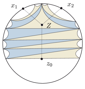
Figure 11. Two paths of tripods

Proof.

The process is clear from Picture (11). Let us make it formal. Let $x_{1}$ and $x_{2}$ be two points in ${\bf P}^{1}(\mathbb{R})$ and assume that $d_{z_{0}}(x_{1},x_{2})$ is small enough. If $x_{1}\not=x_{2}$, we can now find three geodesic arcs $\gamma_{0}$, $\gamma_{1}$ and $\gamma_{2}$ joining in a point $Z$ in ${\bf H}^{2}$ with angles $2\pi/3$ so that their other extremities are respectively $z_{0}$, $x_{1}$ and $x_{2}$. The arc $\gamma_{0}$ is oriented from $z_{0}$ to $Z$, whilst the others are from $Z$ to $x_{i}$ respectively. The tripod $\tau^{0}$ orthogonal to all three geodesic arcs $\gamma_{0}$, $\gamma_{1}$, and $\gamma_{2}$ will be referred in this proof as the forking tripod and the point of intersection of $\gamma_{i}$ with $\tau^{0}$ is denoted $y_{i}$.

Observe now that there exists a universal positive constant $\boldsymbol{\kappa}_{1}$ so that

$${\operatorname{length}}(\gamma_{0})=d_{{\bf H}^{2}}(z_{0},Z)\geqslant-2\boldsymbol{\kappa}_{1}\log\left(d_{z_{0}}(x_{1},x_{2})\right)\ ,$$ (50)

where $d_{{\bf H}^{2}}$ is the hyperbolic distance. We now construct a (discrete) lamination $\Gamma$ with the following properties

1. $\Gamma$ contains the three sides of the forking tripod, and $z_{0}$ is in the support of $\Gamma$.

2. All geodesics in $\Gamma$ intersect orthogonally, either $\gamma_{0}$, $\gamma_{1}$ or $\gamma_{2}$. Let $X$ be the set of these intersection points.

3. The distance between any two successive points in $X$ (for the natural ordering of $\gamma_{0}$, $\gamma_{1}$ and $\gamma_{2}$) is greater than 1 and less than 2.

We orient each geodesic in $\Gamma$ so that its intersection with $\gamma_{0}$, $\gamma_{1}$ or $\gamma_{2}$ is positive. We may now construct two sequences of geodesics $\Gamma^{1}$ and $\Gamma^{2}$ so that $\Gamma^{i}$ contains all the geodesics in $\Gamma$ that are encountered successively when going from $z_{0}$ to $x_{i}$.

For two successive geodesics $\gamma_{i}$ and $\gamma_{i+1}$ – in either $\Gamma^{1}$ or $\Gamma^{2}$ – we consider the associated finite paths of tripods given by the following construction:

1. In the case $\gamma_{i}$ and $\gamma_{i+1}$ are both sides of the forking tripod:, the path consists of just one tripod: the forking tripod

2. In the other case: we consider the path of tripods with two elements $\tau_{i}$ and $\hat{\tau}_{i}$ where

   $$\tau_{i} = (\gamma_{i}(-\infty),\gamma_{i}(+\infty),\gamma_{i+1}(+\infty))\ ,$$

   $$\tau_{i+1} = (\gamma_{i}(-\infty),\gamma_{i+1}(+\infty),\gamma_{i+1}(-\infty))\ .$$

Combining these finite paths of tripods in infinite sequences one obtains two sequences of tripods $\underline{T}^{i}=\{T^{i}_{m}\}_{m\in\mathbb{N}}$, with $i\in\{1,2\}$ which coincides up to the first $-\boldsymbol{\kappa}_{1}\log\left(d_{z_{0}}(x_{1},x_{2})\right)$ tripods. Moreover the swish between $T_{m}^{i}$ and $T^{i}_{m+1}$ is bounded by a universal constant $\boldsymbol{\kappa}_{2}$ – of which actual value we do not care, since obviously the set of configurations $(T_{m}^{i},T^{i}_{m+1})$ is compact (up to the action of $\mathsf{SL}_{2}(\mathbb{R})$).

An easy check shows that these sequences of tripods are 3-sequences. The last condition is immediate after possibly enlarging the value of $\boldsymbol{\kappa}_{2}$ obtained previously. ∎

8.2.2. Sullivan curves as deformations

Let $z_{0}$, $x_{1}$, $x_{2}$, $\underline{T}^{1}$ and $\underline{T}^{2}$ be as in Lemma 8.2.1. Let $\xi$ be an $\zeta$-Sullivan map. The main idea is that $\xi$ will define a deformation of the sequences of tripods. Our first step is the following lemma

Lemma 8.2.2.

For every positive $\varepsilon$, there exists $\zeta$, so that for every $i\in\{1,2\}$ and $m\in\mathbb{N}$ there exist a compatible tripod $\tau^{i}_{m}$ for $T^{i}_{m}$ with respect to $\xi$, with associated circle maps $\eta^{i}_{m}$ and extended circle maps $\nu^{i}_{m}$, so that denoting by $d_{m}^{i}$ the metric $d_{\tau^{i}_{m}}$ we have

$$\partial^{\pm}\tau^{i}_{m} = \xi(\partial^{\pm}T^{i}_{m})\ ,$$ (51)

$$d_{m}^{i}(\xi,\eta^{i}_{m}) \leqslant \varepsilon\ ,$$ (52)

$$d(\tau^{i}_{m},\nu^{i}_{m-1}(T^{i}_{m})) \leqslant \varepsilon\ .$$ (53)

Moreover for all $m$ smaller than $-\boldsymbol{\kappa}_{1}\log d_{z_{0}}(x_{1},x_{2})$, we have $\tau^{1}_{m}=\tau^{2}_{m}$.

Proof.

Let us construct inductively the sequence $\underline{\tau}_{i}$ . Let us first construct $\tau^{1}_{0}=\tau^{2}_{0}$. We first choose a compatible tripod for $T_{0}$, with associated circle maps $\eta^{1}_{0}=\eta^{2}_{0}$ and extended circle maps $\nu^{1}_{0}=\nu^{2}_{0}$. Let $\tau_{0}^{i}=\eta_{0}^{i}(T_{0})$ so that denoting by $d_{0}^{i}$ the metric $d_{\tau^{i}_{0}}$, we have the inequality

$$d^{i}_{0}(\xi,\eta^{i}_{0})\leqslant\zeta\ .$$ (54)

In particular

$$d_{0}^{i}(\partial^{\pm}\tau^{i}_{0},\xi(\partial^{\pm}T^{i}_{0}))\leqslant\zeta\,.$$

we may thus slightly deform $\eta^{i}_{0}$ (with respect to the metric $d^{i}_{0}$) so that assertion (51) holds. Then for $\zeta$ small enough, the relation (52) holds for $m=0$, where $\varepsilon=2\zeta$

Assume now that we have built the sequence up to $\tau^{i}_{m-1}$. Let then

$$\tau_{1}=\tau^{i}_{m-1}\ ,\ \ T_{1}=T^{i}_{m-1}\ ,\ \ T_{2}=T^{i}_{m}\ ,$$

and finally $\nu_{1}=\nu^{i}_{m-1}$. Recall that by the construction of $T_{1}$ and $T_{2}$,

$$d(T_{1},T_{2})\leqslant\boldsymbol{\kappa}_{2}\eqqcolon M\ ,\ \ d(\nu_{1}(T_{1}),\tau_{1})\leqslant\varepsilon\ .$$

We may now apply the second part of Lemma 8.1.6, which shows that given $\varepsilon$ and $\zeta$ small enough, we may choose a compatible tripod $\tau_{2}$ for $T_{2}$ with respect to $\xi$ so that,

$$d(\tau_{2},\nu_{1}(T_{2}))\leqslant\frac{1}{2}\varepsilon\ .$$

We now set $\tau^{i}_{m}\eqqcolon\tau_{2}$, possibly deforming it a little so that assertion (51) holds. Then by the definition of compatibility assertion (52) holds, while assertion (53) is by construction. The last part of the lemma follows from the inductive nature of our construction and some bookkeeping. ∎

8.2.3. Main result

Let $\xi$ be a $\zeta$-Sullivan curve. We use the notation of the two previous lemmas. Our main result is

Proposition 8.2.3.

For all positive $\varepsilon$, for $\zeta$ small enough,

1. the quadruples $\theta_{m}^{i}\coloneqq\left(\tau^{i}_{m},\xi(\partial T^{i}_{m})\right)$ are reduced $\varepsilon$-quasi-tripods.

2. If $T^{i}_{m}$ and $T^{i}_{m+1}$ are $R^{i}_{m}$-swished then $\theta^{i}_{m}$ and $\theta^{i}_{m+1}$ are $(R^{i}_{m},\varepsilon)$-swished.

3. The sequences $\underline{\theta}^{1}$ and $\underline{\theta}^{2}$ are $\varepsilon$-deformations of the sequence $\nu_{0}(\underline{T}^{1})$ and $\nu_{0}(\underline{T}^{2})$ respectively.

4. The $n$ first elements of $\underline{\theta}^{1}$ and $\underline{\theta}^{2}$ coincide for $n$ equal $-\boldsymbol{\kappa}_{1}\log(d_{z_{0}}(x_{1},x_{2}))$.

5. For all $m$, $\xi(x_{i})$ belongs to the sliver $S_{\varepsilon}(\tau^{i}_{m})$.

Proof.

Equation (54) guarantees that $\theta^{i}_{m}$ is a $\zeta$-quasi tripod and reduced by condition (51). Furthermore since $T^{i}_{m}$ is at most $\boldsymbol{\kappa}_{2}$ swished from $T^{i}_{m-1}$ by Proposition 8.2.1, inequality (53) implies that $\theta^{i}_{m+1}$ is at most $(R^{i}_{m},\varepsilon)$-swished from $\theta^{i}_{m}$, and thus $\underline{\tau}^{i}$ is a model for $\underline{\theta}^{i}$. Statement (iii) then follows from Proposition 4.3.1. The coincidence up to $-\boldsymbol{\kappa}_{1}\log(d_{z_{0}}(x_{1},x_{2}))$. follows from the last part of Lemma 8.2.2. Let us prove the last item in the proposition. By the $\zeta$-Sullivan condition

$$d^{i}_{m}(\xi(x^{i}),\eta^{i}_{m}(x^{i}))\leqslant\zeta.$$

Let $x^{i}_{m}$ be the $\mathsf{SL}_{2}(\mathbb{R})$-tripod as in Proposition 8.2.1, let $\sigma^{i}_{m}=\nu^{i}_{m}(x^{i}_{m})$ and $\underline{d}^{i}_{m}\coloneqq d_{\sigma^{i}_{m}}.$. By construction, $\sigma^{i}_{m}$ and $\tau_{i}^{m}$ are coplanar By statement (iv) of Lemma 8.2.1 , $d(x^{i}_{m},T^{i}_{m})$ is bounded by a constant $\boldsymbol{\kappa}_{2}$, thus by Proposition 3.4.4 $d^{i}_{m}$ and $\underline{d}^{i}_{m}$ are uniformly equivalent by constants only depending on ${\mathsf{G}}$ and $\boldsymbol{\kappa}_{2}$. Thus for $\zeta$ small enough we have

$$\underline{d}^{i}_{m}(\xi(x^{i}),\partial^{0}\sigma^{i}_{m})=\underline{d}^{i}_{m}(\xi(x^{i}),\eta^{i}_{m}(x^{i}))\leqslant\varepsilon\ .$$

In other words, $\xi(x^{i})$ belongs to the cone $C_{\varepsilon}(\sigma^{i}_{m})$ hence to the sliver $S_{\varepsilon}(\hat{\tau}^{i}_{m})$ as required, since $\sigma^{i}_{m}$ and $\tau_{i}^{m}$ are coplanar and $\partial^{\pm}\sigma^{i}_{m}=\partial^{\pm}\tau^{i}_{m}$. ∎

8.2.4. Limit points

Let then $\Gamma^{i}_{m}$ be the chords generated by the tripods $\hat{\theta}^{i}_{2m}$, and let us consider the sequences of chords $\underline{\Gamma}_{i}\coloneqq\{\Gamma^{i}_{m}\}_{m\in\mathbb{N}}$. The final part of our construction is the following lemma

Lemma 8.2.4.

The sequence of chords $\underline{\Gamma}^{i}$ are $(1,\varepsilon)$-deformed sequences of cuffs for $\zeta$ small enough. Furthermore these two sequences coincides up to $N>-\boldsymbol{\kappa}_{1}d_{\tau}(z_{1},z_{2})$. Finally

$$\bigcap_{m=0}^{\infty}\underline{\Gamma}^{i}=\{\xi(x_{i})\}$$ (55)

Proof.

The first two items of Proposition 8.2.3, together with Proposition 4.3.1 implies that for $\zeta$ small enough the sequence $\underline{\theta}^{i}$ are $\varepsilon$-deformations of the model sequences $\nu_{0}\left(\underline{T}^{i}\right)$. This implies the first two assertions. Equation (55) follows by Theorem 7.2.1 (taking $\ell_{0}=R=1$ and $\beta={\rm A}$), and the last item of Proposition 8.2.3. ∎

8.3. Sullivan curves and the Hölder property

We prove a more precise version of Theorem 8.1.2 that we state now

Theorem 8.3.1.

[Hölder modulus of continuity] There exists positive constants ${\rm M}$, $\zeta_{0}$ and $\alpha$ so that given a $\zeta_{0}$-Sullivan map $\xi$ from ${\bf P}^{1}(\mathbb{R})$ to ${\bf F}$, then for every tripod $T$ in ${\bf P}^{1}(\mathbb{R})$, with associated $\mathsf{G}$-tripod $\tau$, with respect to $\xi$, we have

$$d_{\tau}(\xi(x),\xi(y))\leqslant{\rm M}\cdotp d_{T}(x,y)^{\alpha}\ ,$$

Proof.

Since $d_{\tau}$ has uniformly bounded diameter, It is enough to prove this inequality, for $T$ so that $d_{T}(x,y)$ is small enough. Let then $x_{1}=x$, $x_{2}=x$ be in ${\bf P}^{1}(\mathbb{R})$ and $z_{0}=s(T)$, $\xi$ a $\zeta$-Sullivan map (for $\zeta$ small enough) and ${\underline{T}}^{i}$, $\underline{\tau}_{i}$, the sequences of $\mathsf{SL}_{2}(\mathbb{R})$-tripods and ${\mathsf{G}}$-tripods constructed in the preceding section, let $\underline{\Gamma}_{i}$ the sequence of chords satisfying Lemma 8.2.4. Let

$$\tau_{0}\coloneqq\tau^{1}_{0}=\tau^{2}_{0},\ \ \nu_{0}\coloneqq\nu^{1}_{0}=\nu^{2}_{0}\ ,\ T_{0}\coloneqq T^{1}_{0}=T^{2}_{0}$$

Let $N>-\boldsymbol{\kappa}_{1}\log(d_{T_{0}}(x_{1},x_{2}))$ so that $\underline{\tau}^{1}$ and $\underline{\tau}^{2}$ coincide up to the first $N$ tripods. By Theorem 7.2.1 using Lemma 8.2.4, we have

$$d_{\tau_{0}}(\xi(x_{1}),\xi(x_{2}))\leqslant{\rm q}^{N}\cdotp{\rm A}\leqslant{\rm B}\cdotp d_{z_{0}}(x_{1},x_{2})^{\boldsymbol{\alpha}}={\rm B}\cdotp d_{T_{0}}(x_{1},x_{2})^{\boldsymbol{\alpha}}\,$$ (56)

for some positive constants ${\rm B}$ and ${\boldsymbol{\alpha}}$ only depending on ${\rm q}$, ${\rm A}$ and $\boldsymbol{\kappa}_{1}$.

Here $\tau_{0}$ is associated to $T_{0}$. But since $d(T_{0},T)$ is uniformly bounded, by the first assertion in Lemma 8.1.6, $d(\tau_{0},\tau)$ is uniformly bounded (for $\zeta$ small enough), thus by Proposition 3.4.4, $d_{\tau}$ and $d_{\tau_{0}}$ are uniformly equivalent. In particular,

$$d_{\tau}(\xi(x),\xi(y))\leqslant{\rm F}\cdotp d_{\tau_{0}}(\xi(x),\xi(y))\leqslant{\rm M}\cdotp d_{T}(x,y)^{\alpha}\ .$$

This concludes the proof.∎

8.4. Sullivan curves and the Anosov property

In this section, let $\xi$ be a $\zeta$-Sullivan map equivariant under the action of a cocompact Fuchsian group $\Gamma$ for a representation $\rho$ of $\Gamma$ in ${\mathsf{G}}$.

8.4.1. A short introduction to Anosov representations

Intuitively, a hyperbolic group is $\mathsf{P}$-Anosov if every element is $\mathsf{P}$-loxodromic, with “contraction constant” comparable with the word length of the the group.

Let us be more precise, let $\mathsf{P}^{+}$ be a parabolic and $\mathsf{P}^{-}$ its opposite associated to the decomposition

$$\mathfrak{g}=\mathfrak{n}^{+}\oplus\mathfrak{l}\oplus\mathfrak{n}^{-}\ ,\ \ \mathfrak{p}^{\pm}=\mathfrak{n}^{\pm}\oplus\mathfrak{l}$$

For a hyperbolic surface $S$, let $\mathsf{U}S$ be its unit tangent bundle equipped with its geodesic flow $h_{t}$. Let $\rho$ be a representation of $\pi_{1}(S)$ into $\mathsf{G}$. Let $\mathfrak{G}_{\rho}$ be the flat Lie algebra bundle over $S$ with monodromy $\operatorname{Ad}\circ\rho$. The action of $h_{t}$ lifts by parallel transport the action of a flow $H_{t}$ on $\mathfrak{g}_{\rho}$. We say that the action is Anosov if we can find a continuous splitting into vector sub-bundles, invariant under the action of $H_{t}$

$$\mathfrak{G}_{\rho}=\mathfrak{N}^{+}\oplus\mathfrak{l}\oplus\mathfrak{N}^{-},$$

such that

• at each point $x\in\mathsf{U}S$, the splitting is conjugate to the splitting $\mathfrak{g}=\mathfrak{p}^{+}\oplus\mathfrak{l}\oplus\mathfrak{p}^{-}$,

• The action of $H_{t}$ is contracting towards the future on $\mathfrak{N}^{+}$ and contracting towards the past on $\mathfrak{N}^{-}$

Equivalently let $\mathsf{F}^{\pm}_{\rho}$ be the associated flat bundles to $\rho$ with fibers $\mathsf{G}/\mathsf{P}^{\pm}$. The action of $h_{t}$ lifts to an action denoted $H_{t}$ by parallel transport. Then, the representation $\rho$ is Anosov, if we can find continuous $\rho$-equivariant maps $\xi^{\pm}$ from $\partial_{\infty}\pi_{1}(S)$ into $\mathsf{G}/\mathsf{P}^{\pm}$ so that

• for $x\not=y$, $\xi^{+}(x)$ is transverse to $\xi^{-}(y)$,

• the associated sections $\Xi^{\pm}$ of $\mathsf{F}^{\pm}$ over $\mathsf{U}S$ by $\rho$ are attracting points, respectively towards the future and the past, for the action of $H_{t}$ on the space of sections endowed with the uniform topology.

8.4.2. A preliminary lemma

For a tripod $\tau$, let $\tau^{\perp}$ be the coplanar tripod to $\tau$ so that $\tau^{\perp}$ is obtained after a $\pi/2$ rotation of $\tau$ with respect to $s(\tau)$. In other words, $\partial\tau^{\perp}=(\partial^{0}\tau,x,\partial^{+}\tau)$ where $x$ is the symmetric of $\partial^{0}\tau$ with respect to the geodesic whose endpoints are $\partial^{-}\tau$ and $\partial^{+}\tau$. Observe that $s(\tau)=s(\tau^{\perp})$ and thus $d_{\tau}=d_{\tau^{\perp}}$.

Our key lemma is the following

Lemma 8.4.1.

There exists $\boldsymbol{\zeta}$ with such that if $\xi$ is a $\boldsymbol{\zeta}$-Sullivan map, then there exists positive constants $R$ and $c$ so that if $T$ is a tripod in $\mathsf{SL}_{2}(\mathbb{R})$, then for any $\tau$ and $\sigma$ compatible tripods (with respect to $\xi$) to $T$ and $\varphi_{R}(T)$ satisfying

$$\partial^{+}\sigma=\partial^{+}\tau=\xi(\partial^{+}T)\ ,$$

we have

$$\forall x,y\in C_{c}(\sigma^{\perp}),\ \ d_{\tau^{\perp}}(x,y)\leqslant\frac{1}{2}\cdotp d_{\sigma^{\perp}}(x,y)\ .$$

In this lemma, $\xi$ does not have to be equivariant. Observe also, that with the notation of the lemma $\partial^{0}(\sigma^{\perp})=\xi(\partial^{+}T)$.

Proof.

We will use the Confinement Lemma 6.0.1. Let then, using the notation of the Confinement Lemma, $b\coloneqq\beta_{3}$, and $\ell_{0}$ an integer greater than $\ell(\beta_{3})$, and $\eta_{0}$ as in the conclusion of the lemma.

Let $z_{0}\coloneqq s(T)$ be the orthogonal projection of $\partial^{0}T$ on the geodesic joining $\partial^{-}T$ to $\partial^{+}T$. Let $x_{1}=x_{2}\coloneqq\partial^{+}T$. Let us now construct, for $\varepsilon\leqslant\frac{\eta_{0}}{2\ell_{0}}$ and $\boldsymbol{\zeta}$ small enough as in paragraphs 8.2 and 8.2.2

• The sequence of $\mathsf{SL}_{2}(\mathbb{R})$-tripods $\underline{T}\coloneqq\underline{T}^{1}=\underline{T}^{2}$ with $T_{0}=T^{\perp}$, associated to the coplanar sequence of chords $\underline{h}$,

• The tripods $\tau_{m}\coloneqq\tau^{1}_{m}=\tau^{2}_{m}$, and the corresponding sequence of reduced $\varepsilon$-quasi tripods $\underline{\theta}\coloneqq\underline{\theta}^{1}=\underline{\theta}^{2}$, which is an $\varepsilon$-deformation of $\nu_{0}(\underline{\tau})$ – according to Proposition 8.2.3 – and associated to the deformed sequence of chords $\underline{\Gamma}$,

• we also denote by $\nu_{i}$ the extended circle map associated to $T_{i}$ that satisfies $\nu(T_{i})=\tau_{i}$. Let us also denote by $\mu_{i}$ the $\mathsf{SL}_{2}(\mathbb{R})$-tripods which is the projection of $h_{2(i+1)}$ on $h_{2i}$, and

  $$\lambda_{i}\coloneqq\nu_{2i\ell_{0}}(\mu_{i\ell_{0}}).$$

It follows that $T_{2\ell_{0}m},\ldots,T_{2\ell_{0}(m+1)}$ is a strong $(\ell_{0},2\ell_{0})$-coplanar path of tripods. And thus according to the Confinement Lemma 6.0.1 and our choice of constants, $(\Gamma_{2\ell_{0}m},\Gamma_{2\ell_{0}(m+1)})$ is $(b,\boldsymbol{\kappa}^{7})$-squeezed and its commanding tripod is the projection of $\nu_{2\ell_{0}m}(h_{2\ell_{0}{m+1}})$ on $\nu_{2\ell_{0}m}(h_{2\ell_{0}m})$ that is $\lambda_{m}$. In other words, since $\lambda_{m+1}\in S_{0}(\nu_{2\ell_{0}m}(h_{2\ell_{0}m}))$ we have for all $m$

$$C_{b}(\lambda_{m})\prec\boldsymbol{\kappa}^{7}C_{\boldsymbol{\kappa}^{7}b}(\lambda_{m+1})$$

Thus by Corollary 5.1.3, using the fact that $\beta_{3}\leqslant\alpha_{3}$, where $\alpha_{3}$ is the constant in Proposition, we have

$$\forall u,v\in C_{b}(\lambda_{n}),\ d_{\lambda_{0}}(u,v)\leqslant\frac{1}{2^{n}}d_{\lambda_{n}}(u,v)\ .$$ (57)

We now make the following claim

Claim1: there exists a constant $N$ only depending in ${\mathsf{G}}$ so that for any tripod $\beta$ compatible with $\varphi_{2n\ell_{0}}(T)$ then

$$d(\beta^{\perp},\lambda_{n})\leqslant N\,.$$ (58)

Elementary hyperbolic geometry first shows that there exist positive constants $N_{1}$ and $M_{2}$ so that

$$d(\lambda_{n},\tau_{2n\ell_{0}})=d(\mu_{n\ell_{0}},T_{2n\ell_{0}}) \leqslant N_{1}\ ,$$

$$d(\varphi_{2n\ell_{0}}(T),T_{2n\ell_{0}}) \leqslant M_{2}.$$

By Lemma 8.1.6, there exists a constant $N_{2}$ so that

$$d(\beta,\tau_{2n\ell_{0}})\leqslant N_{2}\ ,$$

Since there exists a constant $N_{3}$ so that $d(\beta,\beta^{\perp})\leqslant N_{3}$, The triangle inequality yields the claim. inequality (58) and Proposition 3.4.4 yields that there exists a constant $C$ so that if $\sigma_{n}$ is compatible with $\varphi_{n\ell_{0}}(T)$, then

$$\frac{1}{C}d_{\sigma^{\perp}_{n}}\leqslant d_{\lambda_{n}}\leqslant Cd_{\sigma^{\perp}_{n}}\ .$$ (59)

Then taking $n_{0}$ so that $2^{n_{0}-1}>C^{2}$, $R=n_{0}\ell_{0}$, we get from inequality (57)

$$\forall x,y\in C_{b}(\lambda_{n_{0}}),\ \ d_{\tau^{\perp}}(x,y)\leqslant\frac{1}{2}\cdotp d_{\sigma^{\perp}}(x,y)\ .$$

To conclude, it is therefore enough to prove that

Final Claim : There exists a constant $c$ only depending on ${\mathsf{G}}$ so that

$$C_{c}(\sigma^{\perp})\subset C_{b}(\lambda_{n_{0}})\ .$$

Recall that by hypothesis, $\partial^{+}(\sigma)=\xi(x)$. By the last item in Proposition 8.2.3, for $\zeta$ small enough

$$\partial^{0}(\sigma^{\perp})=\xi(x)\in S_{b/2}(h_{n})\ ,$$

for all $n$. By the squeezing property, it follows that $\xi(x)\in C_{b/2}(\lambda_{m})$ for all $m$.

Since $d_{\lambda_{n_{0}}}$ and $d_{\sigma^{\perp}}$ are uniformly equivalent by inequality (59), we obtain, taking$c=b(2C)^{-1}$,

$$C_{c}(\sigma^{\perp})=\{u\in{\bf F},d_{\sigma^{\perp}}(u,\xi(x))\leqslant c\}\subset\{u\in{\bf F},d_{\lambda_{n_{0}}}(u,\xi(x))\leqslant b/2\}=C_{b}(\lambda_{n_{0}})\ .$$

This concludes the proof of the final claim, hence of the lemma. ∎

8.4.3. Completion of the proof of Theorem 8.1.3

The proof is now standard. Let $\rho$ be a representation of a cocompact torsion free Fuchsian group $\Gamma$. Let $\mathcal{S}$ be the space of $\mathsf{SL}_{2}(\mathbb{R})$ tripods, $U=\Gamma\backslash\mathcal{S}$ the space of tripods in the quotient equipped with the flow $\varphi$. The space $U$ with its flow $U$ is naturally conjugate to the geodesic flow of the underlying hyperbolic surface. Let finally $\mathcal{F}$ be the $\rho$-associated flat bundle over $U$ with fiber ${\bf F}$. This fiber bundle is equipped with a flow $\{\Phi_{t}\}_{t\in\mathbb{R}}$ lifting the flow $\{\varphi_{t}\}_{t\in\mathbb{R}}$ by parallel transport along the orbit.

Let $\xi$ be a $\rho$-equivariant $\zeta$-Sullivan map for $\zeta$ small enough so that Lemma 8.4.1 holds. Observe that $\xi$ give now rise to two transverse $\Phi_{t}$-invariant sections of ${\bf F}$:

$$\sigma^{+}(T)\coloneqq\xi(\partial^{+}T)\ , \sigma^{-}(T)\coloneqq\xi(\partial^{-}T)\$$

These sections are transverse for $\zeta$ small enough: more precisely for $\zeta<k/2$, where $k=d_{\tau}(\partial^{+}\tau,\partial^{-}\tau)$ for any tripod $\tau$.

We now choose a fiberwise metric $d$ on $\mathcal{F}$ as follows: for every $T\in\mathcal{S}$, let $\tau(T)$ be a compatible tripod. We may choose the assignment $T\mapsto\tau(T)$ to be $\Gamma$-invariant. We define our fiberwise metric at $T$ to be $d_{T}\coloneqq d_{\tau(T)}$. This metric may not be continuous transversely to the fibers, but it is locally bounded: locally at a finite distance to a continuous metric since the set of compatible tripods has a uniformly bounded diameter by Lemma 8.1.6.

Now, lemma 8.4.1 exactly tells us that $\sigma^{+}$ is a attracting fixed section of $\{\phi_{t}\}_{t\in\mathbb{R}}$ towards the future, and by symmetry that $\sigma^{-}$ is a attracting fixed section of $\{\phi_{t}\}_{t\in\mathbb{R}}$ towards the past. By definition, $\rho$ is ${\bf F}$-Anosov and this concludes the proof of Theorem 8.1.3

8.4.4. Anosov and Sullivan Lemma

As an another relation of the Anosov property and Sullivan curves, let us prove the following

Lemma 8.4.2.

Let $\rho_{0}$ be an Anosov representation of a Fuchsian group $\Gamma$. Assume that the limit map $\xi_{0}$ is $\zeta$-Sullivan, then, for any positive $\varepsilon$, any nearby representation to $\rho$ is Anosov with a $(\zeta+\varepsilon)$-Sullivan limit map.

Proof.

By the stability property of Anosov representations [20, 12] any nearby representation $\rho$ is Anosov. Let $\xi_{\rho}$ be its limit map.

By Guichard–Wienhard [12] – see also [6] – $\xi_{\rho}$ depends continuously on $\rho$ in the uniform topology. More precisely, for any positive $\varepsilon$, for any tripod $\tau$ for $\mathsf{G}$, there exists a neighborhood $U$ of $\rho_{0}$, so that for all $\rho$ in $U$, for all $x\in\partial_{\infty}{\bf H}^{2}$,

$$d_{\tau}(\xi_{\rho}(x),\xi_{\rho_{0}}(x))\leqslant\varepsilon\ .$$ (60)

Instead of fixing $\tau$, we may as well assume that $\tau$ belongs to a bounded set $K$ of $\mathcal{G}$, using for instance Proposition 3.4.4.

Let us consider a compact fundamental domain $D$ for the action of $\Gamma$ on the space of tripods with respect to ${\bf H}^{2}$. For every tripod $T$ in $D$, we have a compatible $\mathsf{G}$-tripod $\tau_{\mathsf{T}}$ with circle map $\nu_{T}$ with respect to $\xi_{0}$. Then by Lemma 8.1.6, the set

$$D_{\mathsf{G}}:=\{\tau_{T}\mid T\in D\}\ ,$$

is bounded. Thus inequality (60) holds for all $\tau$ in $D_{\mathsf{G}}$ . It follows that for all $T\in D$,

$$d_{\tau_{T}}(\xi_{\rho}(x),\eta_{T}(x))\leqslant\zeta+\varepsilon\ .$$ (61)

Using the equivariance under $\Gamma$, the inequality (61) now holds for all tripods $T$ for ${\bf H}^{2}$. In other words, $\xi_{\rho}$ is $(\zeta+\varepsilon)$-Sullivan. ∎

8.5. Improving Hölder derivatives

Our goal is to explain that under certain hypothesis we can can promote a Sullivan curve with respect to a smaller subset to a full Sullivan curve. We need a series of technical definitions before actually stating our theorem

1. For every tripod $T$ for ${\bf H}^{2}$, let $d_{T}$ be the visual distance on $\partial_{\infty}{\bf H}^{2}$ associated to $T$. We say a subset $W$ of $\partial_{\infty}{\bf H}^{2}$ is $(a,T)$-dense if

   $$\forall x\in\partial_{\infty}{\bf H}^{2},\ \exists y\in W,\ d_{T}(x,y)\leqslant a$$ (62)

2. Let $a$ and $\zeta$ be a positive number, $Z$ a dense subset of $\partial_{\infty}{\bf H}^{2}$. Let us say a map $\xi$ from $\partial_{\infty}{\bf H}^{2}$ to ${\bf F}$ is $(a,\zeta)$-Sullivan if given any tripod $T$ in ${\bf H}^{2}$, there exists

   • a circle map $\xi_{T}$,

   • an $(a,T)$-dense subset $W_{T}$ of $Z$,

   so that, writing $\tau\coloneqq\xi_{T}(T)$, we have for all $x$ in $W_{T}$, $d_{\tau}(\xi_{T}(x),\xi(x))\leqslant\zeta$.

3. Let $\Gamma$ a be cocompact Fuchsian group and $\rho$ a representation of $\Gamma$ in $\mathsf{G}$. Let $\xi$ be a $\rho$-equivariant map from $\partial_{\infty}{\bf H}^{2}$ to $F$. We say $\xi$ is attractively coherent if given any $y$ point in $\partial_{\infty}{\bf H}^{2}$, there exists a sequence $\{{\gamma}_{m}\}_{m\in\mathbb{N}}$ of elements of $\Gamma$ such that

   • the limit of $\{\gamma^{+}_{m}\}_{m\in\mathbb{N}}$ is $y$,

   • $\xi(y)$ is the limit of $\{{z}_{m}\}_{m\in\mathbb{N}}$, where $z_{m}$ is an attractive fixed point for $\rho(\gamma_{m})$.

Our Improvement Theorem is the following

Theorem 8.5.1.

[Improvement Theorem] Let $\Gamma$ be a cocompact Fuchsian group. Then there exists a positive constant $\zeta_{2}$ and there exists a positive $a_{0}$ such that given

1. a continuous family of representations $\{\rho_{t}\}_{t\in[0,1]}$ of $\Gamma$ in $\mathsf{G}$,

2. an $(a_{0},\zeta$)-Sullivan map $\xi_{t}$, with $\zeta\leqslant\zeta_{2}$, attractively coherent, and $\rho_{t}$ equivariant for each $t\in[0,1]$. Assume also that $\xi_{0}$ is $2\zeta$-Sullivan,

Then for all $t$, $\xi_{t}$ is a $2\zeta$-Sullivan map.

8.5.1. Bootstrapping and the proof of Theorem 8.5.1

Let us first start with a preliminary lemma

Lemma 8.5.2.

Let $\rho$ be an Anosov representation of a Fuchsian group. Let $\xi$ be an attractively coherent map from $\partial_{\infty}{\bf H}^{2}$ to ${\bf F}$. Then $\xi$ is the limit map of $\rho$.

Proof.

Let $\eta$ be the limit map of $\rho$. Let $y\in\partial_{\infty}{\bf H}^{2}$. Let $\{{\gamma}_{m}\}_{m\in\mathbb{N}}$ be as in the definition of attractively continuous. Since $\gamma^{+}_{m}$ is the attractive fixed point of $\gamma$, it follows that $\eta(\gamma^{+}_{m})=z_{m}$. The continuity of $\eta$ shows that $\eta(y)=\xi(y)$. ∎

We may now proceed to the proof. Let $\{\xi_{t}\}_{t\in[0,1]}$, $\{\rho_{t}\}_{t\in[0,1]}$, and $\Gamma$ as in the hypothesis of the theorem that we want to prove. Let $\zeta_{0}$, ₀, $\alpha$ be as in Theorem 8.3.1. Let $\zeta_{1}$ so that Theorem 8.1.3 holds. Let finally $\zeta_{2}=\frac{1}{4}\min(\zeta_{1},\zeta_{0})$ and $\zeta\leqslant\zeta_{2}$.

Let us consider the subset $K$ of $[0,1]$ of those parameters $t$ so that $\xi_{t}$ is $2\zeta$-Sullivan.

Lemma 8.5.3.

The set $K$ is closed.

Proof.

Let $\{{t}_{m}\}_{m\in\mathbb{N}}$ be a sequence of elements of $K$ converging to $s$. For all $n$, $\{\xi_{t_{m}}\}_{m\in\mathbb{N}}$ forms an equicontinuous family by Theorem 8.3.1 since $2\zeta_{2}\leqslant\zeta_{0}$. We may extract a subsequence converging to a map $\hat{\xi}$ which is $\rho_{s}$ equivariant and $\zeta_{2}$-Sullivan. In particular since $2\zeta_{2}\leqslant\zeta_{1}$, it follows that $\rho_{s}$ is Anosov and $\hat{\xi}$ is the limit map of $\rho_{s}$. By hypothesis, $\xi_{s}$ is attractively continuous and thus $\xi_{s}=\hat{\xi}$ by Lemma 8.5.2. This proves that $s\in K$. ∎

We prove that $K$ is open in two steps:

Lemma 8.5.4.

Assume $\xi_{t}$ is $2\zeta$-Sullivan. Then there exists a neighborhood $U$ of $t$ so that for $s\in U$, $\xi_{s}$ is $\zeta_{0}$-Sullivan.

Proof.

Our assumptions guarantee that $\rho_{t}$ is Anosov and by the stability condition for Anosov representations [20, 12] the representation $\rho_{s}$ is Anosov for $s$ close to $t$. Lemma 8.5.2 implies that $\xi_{s}$ is the limit curve of $\rho_{s}$. Lemma 8.1.4 then shows that for $s$ close enough to $t$, $\xi_{s}$ is $\zeta_{0}$-Sullivan since $2\zeta<2\zeta_{2}<\zeta_{0}$. ∎

We now prove a bootstrap lemma:

Lemma 8.5.5.

[Bootstrap] There exists some constant $A$ so that for $a_{0}<A$, if $\xi_{s}$ is $\zeta_{0}$-Sullivan, then $\xi_{s}$ is $2\zeta$-Sullivan

Proof.

This is an easy consequence of the triangle inequality. Since $\xi_{s}$ is $(a_{0},\zeta)$-Sullivan, for every tripod $T$ for ${\bf H}^{2}$, there exists an $a_{0}$-dense subset $W$, a circle map $\eta$ so that for all $y\in W$, $d_{\tau}(\xi_{s}(y),\eta(y))\leqslant\zeta$, where $\tau=\eta(T)$. Let then $x\in\partial_{\infty}{\bf H}^{2}$ and $y\in W$ so that $d_{T}(x,y)\leqslant a_{0}$. Then

$$d_{\tau}(\xi_{s}(x),\eta(x))\leqslant d_{\tau}(\xi(x),\xi(y))+d_{\tau}(\eta(x),\eta(y))+d_{\tau}(\xi(y),\eta(y)\leqslant M_{0}a_{0}^{\alpha_{0}}+a_{0}+\zeta\ .$$

The last quantity is less than $2\zeta$ for $a_{0}$ small enough. This concludes the proof. ∎

Thus $K$ is open: let $t\in K$, then by Lemma 8.5.4, for any nearby $s$ in $K$, $\xi_{s}$ is $\zeta_{0}$-Sullivan hence $2\zeta$ Sullivan by the Bootstrap Lemma 8.5.5. Since $K$ is non empty, closed and open, $K=[0,1]$ and this concludes the proof of the theorem.

9. Pair of pants from triangles

The purpose of this section is to define almost closing pairs of pants. These almost closing pairs of pants will play the role of almost Fuchsian pair of pants in [14]. Section 13 will reveal they are ubiquitous in $\Gamma\backslash\mathcal{G}$.

These almost closing pair of pants are the building blocks for the construction of surfaces whose fundamental group injects. Themselves are built out of two tripods using symmetries, a construction reminiscent of building hyperbolic pair of pants using ideal triangles.

Our main results here will be a result describing the structure of a pair of pantsTheorem 9.2.2 whose proof relies on the Closing Lemma 9.2.1; We will also prove proposition 9.5.1 that gives information onf the boundary loops.

In all this section, $\varepsilon$ and $R$ are positive constants.

9.1. Almost closing pair of pants

Let $\Gamma$ be a subgroup of $\mathsf{G}$. We will consider not only the case of a discrete $\Gamma$ but also the case $\Gamma=\mathsf{G}$.

Given a tripod $\tau_{0}$, the $R$-perfect pair of pants associated to $\tau_{0}$ is the quintuple $(\alpha,\beta,\gamma,\tau_{0},\tau_{1})$ so that $\tau_{0}$ and $\tau_{1}$ are tripods, $\alpha$, $\beta$ and $\gamma$ are elements of $\mathsf{G}$ so that $\alpha\gamma\beta=\operatorname{Id}$, and moreover the pairs $(\tau_{0},\omega^{2}\tau_{1})$, $(\omega(\tau_{0}),\omega\beta(\tau_{1}))$ and $(\omega^{2}(\tau_{0}),\alpha^{-1}\tau_{1})$ are all $R$-sheared.

We also consider alternatively an $R$-perfect pair of pants to be a quadruple $(T,S_{0},S_{1},S_{2})$ so that

$$S_{0}=K\varphi_{R}T\ ,S_{2}=\omega K\phi_{R}(\omega T)\ ,S_{1}=\omega^{2}K\phi_{R}(\omega^{2}T)\ .$$

with the boundary loops $\alpha$, $\beta$ and $\gamma$ so that $S_{0}=\alpha S_{1}$, $S_{2}=\beta S_{0}$ and $S_{1}=\gamma S_{2}$, so that $(\alpha,\beta,\gamma,T,S_{0})$ is a perfect pair of pants with respect to the previous definition.

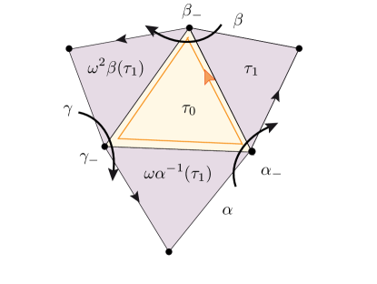
Figure 12. Pair of pants from triangles

More generally we will navigate freely between quadruple of tripods $(T,S_{0},S_{1},S_{2})$ with boundary loops $\alpha$, $\beta$ and $\gamma$ so that $S_{0}=\alpha S_{1}$, $S_{2}=\beta S_{0}$ and $S_{1}=\gamma S_{2}$, and quintuple $(\alpha,\beta,\gamma,T,S_{0})$ where $\alpha$, $\beta$ and $\gamma$ are elements of $\mathsf{G}$ so that $\alpha\gamma\beta=\operatorname{Id}$ using the construction described above in the particular case of $R$-perfect pair of pants.

We now wish to deform that perfect situation.

Let $K$ be the map $x\to\omega(\overline{x})$ defined in paragraph 3.3.1.

Definition 9.1.1.

[Almost closing]

1. Let $T$ and $S$ be two tripods in $\mathcal{G}$, $\alpha$ an element in $\mathsf{G}$ and $\mu$ a positive constant. We say $T$, $S$ are $(\mu,R)$-almost closing for $\alpha$ if there exist tripods $u$ and $v$ so that

   $$d(u,T)\leqslant\mu\ \ d(v,S)\leqslant\mu\ ,$$ , (63)

   $$d(K\circ\varphi_{R}(u),S)\leqslant\mu\ \ d(K\circ\varphi_{R}(v),\alpha(T))\leqslant\mu\ .$$ , (64)

2. Let $P=(\alpha,\beta,\gamma,\tau_{0},\tau_{1})$ so that $\alpha,\beta,\gamma\in\mathsf{G}$ with $\alpha\gamma\beta=1$, and $\tau_{0},\tau_{1}$ are tripods, we say $P$ is a $(\mu,R)$ almost closing pair of pants if

   1. $\tau_{0},$ and $\tau_{1}$ are $(\mu,R)$-almost closing for $\alpha$,

   2. $\omega^{2}\tau_{0},$ and $\omega\alpha^{-1}(\tau_{1})$ are $(\mu,R)$-almost closing for $\gamma$,

   3. $\omega\tau_{0}$ and $\omega^{2}\beta(\tau_{1})$ are $(\mu,R)$-almost closing for $\beta$.

Let us first make immediate remarks:

Proposition 9.1.2.

if $(T,S)$ are $(\mu,R)$ almost closing for $\alpha$, then $(S,\alpha(T))$ (and then $(\alpha^{-1}(S),T)$) are also almost closing for $\alpha$.

Proof.

For the first item observe that if $(u,v)$ is the pair of tripods working in the definition for $(T,S)$, then $(v,\alpha(u))$ works for $(S,\alpha(T))$. For the second item observe that the pair $(\alpha^{-1}\tau_{1},\tau_{0})$ is $(\mu,R)$-almost closing for $\alpha$: we use $(\alpha_{*}^{-1}\tau^{*}_{1},\tau^{*}_{0})$ for $(u,v)$ in the definition. We apply the first item to get that $(\tau_{0},\tau_{1})$ is $(\mu,R)$-almost closing. The other results for other pairs follows from symmetric considerations. ∎

We observe also the following symmetries

Proposition 9.1.3.

[Symmetries] If $(\alpha,\beta,\gamma,\tau_{0},\tau_{1})$ is an $(\mu,R)$-almost closing of pants, then both

$$\omega\left(\alpha,\beta,\gamma,\tau_{0},\tau_{1}\right)\coloneqq\left(\beta,\gamma,\alpha,\omega(\tau_{0}),\omega^{2}(\beta\tau_{1})\right)\ ,$$

$$(\alpha,\beta^{-1}\alpha^{-1},\beta,\tau_{1},\alpha(\tau_{0}))$$

are also $(\mu,R)$ almost closing.

Proof.

We have that, using the definition of almost closing that

1. $\tau_{1},$ and $\alpha(\tau_{0})$ are $(\mu,R)$-almost closing for $\alpha$, from the first item in the previous proposition.

2. After taking the image by $\alpha$, $\omega^{2}\alpha(\tau_{0}),$ and $\omega(\tau_{1})$ are $(\mu,R)$-almost closing for $\alpha\gamma\alpha^{-1}=\beta^{-1}\alpha^{-1}$, and thus from from the first item in the previous proposition, $\omega(\tau_{1})$ and $\omega^{2}\beta^{-1}(\tau_{0})$ are also $(\mu,R)$-almost closing for $\beta^{-1}\alpha^{-1}$,

3. $\omega\tau_{0}$ and $\omega^{2}\beta(\tau_{1})$ are $(\frac{\varepsilon}{R},R)$-almost closing for $\beta$ and thus from the first item in the previous proposition, $\omega^{2}\tau_{1}$ and $\omega\tau_{0}$ are $(\frac{\varepsilon}{R},R)$-almost closing for $\beta$

This proves the result. ∎

9.2. Closing Lemma for tripods

The first step in the proof of the Closing Pant Theorem is the following lemma

Lemma 9.2.1.

[Closing lemma] There exists constants ${{\bf M}}_{2}$, $\varepsilon_{2}$ and $R_{2}$, so that assuming $T$, $S$ are $(\mu,R)$ almost closing for $\alpha$ for $R>R_{2}$, $\mu\leqslant\varepsilon_{2}$, then

1. $\alpha$ is $\mathsf{P}$-loxodromic,

2. $d_{T}(T^{\pm},\alpha^{\pm})\leqslant{{\bf M}}_{2}(\mu+\exp(-R))$

3. Moreover, if $\tau_{\alpha}=\psi(T,\alpha^{-},\alpha^{+})$, $\sigma_{\alpha}=\Psi(S,\alpha^{-},\alpha^{+})$ then

   $$d(\varphi_{2R}(\tau_{\alpha}),\alpha(\tau_{\alpha})) \leqslant {{\bf M}}_{2}(\mu+\exp(-R))\ ,$$ (65)

   $$d(\varphi_{R}(\tau_{\alpha}),\sigma_{\alpha}) \leqslant {{\bf M}}_{2}(\mu+\exp(-R))\ .$$ (66)

4. $d(T,S)\leqslant 2R$.

In the sequel ${{\bf M}}_{i}$, $R_{i}$ and $\varepsilon_{i}$ will denote positive constants only depending on $\mathsf{G}$.

As an immediate consequence and using Proposition 9.1.3, we get the following structure theorem for almost closing pair of pants:

Theorem 9.2.2.

[Structure of pair of pants] There exist positive constants ${{\bf M}}_{0}$, $\varepsilon_{0}$ and $R_{0}$ only depending on ${\mathsf{G}}$ with the following property. Let $\varepsilon\leqslant\varepsilon_{0}$ and $R\geqslant R_{0}$. Then for any $(\varepsilon,R)$-almost closing pair of pants $(\alpha,\beta,\gamma,\tau_{0},\tau_{1})$, we have that

1. $\alpha$, $\beta$ and $\gamma$ are all $\mathsf{P}$-loxodromic.

2. the quadruples $(\tau_{0},x,y,z)$, with $x\in\{\alpha^{-},\gamma^{+}\}$, $y\in\{\alpha^{+},\beta^{-}\}$ and $z\in\{\gamma^{-},\beta^{+}\}$ and $(\tau_{1},u,v,w),$ with $u\in\{\alpha^{-},\beta^{+}\}$, $v\in\{\alpha^{+},\beta^{-1}(\gamma^{-})\}$ and $w\in\{\beta^{-},\beta^{-1}(\gamma^{+})\}$, are all ${{\bf M}}_{0}(\varepsilon+\exp(-R))$-quasi tripod,

3. Moreover, if $\tau_{\alpha}=\Psi(\tau_{0},\alpha^{-},\alpha^{+})$ and $\sigma_{\alpha}=\Psi(\tau_{1},\alpha^{-},\alpha^{+})$ then

   $$d(\varphi_{2R}(\tau_{\alpha}),\alpha(\tau_{\alpha})) \leqslant {{\bf M}}_{0}(\varepsilon+\exp(-R))\ ,$$ (67)

   $$d(\varphi_{R}(\tau_{\alpha}),\sigma_{\alpha}) \leqslant {{\bf M}}_{0}(\varepsilon+\exp(-R))\ .$$ (68)

Proposition 9.5.1 will give further information on the boundary loops.

9.3. Preliminaries

Our first lemma is essentially a result on hyperbolic plane geometry.

Lemma 9.3.1.

There exists constants $R_{3}$ and ${{\bf M}}_{3}$ so that for $R\geqslant R_{3}$ the following holds. Let $u$ be any tripod. Then $v\coloneqq\varphi_{-2R}\left(\left(K\circ\varphi_{R}\right)^{2}(u)\right)$ satisfies

$$d(v,u) \leqslant {{\bf M}}_{3}\exp{\left(-R\right)}\,$$ (69)

$$d(\varphi_{R}(v),K\circ\varphi_{R}(u)) \leqslant {{\bf M}}_{3}\exp{\left(-R\right)}\,$$ (70)

$$\partial^{-}v = \partial^{-}u$$ (71)

Proof.

There exist a constant $M$, so that for all $w$,

$$d(w,K(w))\leqslant M.$$ (72)

Recall that $w$ and $K(w)$ are coplanar. In the upper half plane model where $\partial^{-}w=\partial^{-}K(w)=\infty$, $K(w)$ is obtained from $w$ by an horizontal translation. Thus, for $R$ large enough,

$$d(\varphi_{-R}(w),\varphi_{-R}(K(w)))\leqslant{{\bf M}}_{3}\exp{\left(-R\right)}.$$

Applying this inequality to $w=\varphi_{R}(K\circ\varphi_{R}(u))$, gives

$$d\left(K\circ\varphi_{R}(u),\varphi_{R}(v)\right)=d\left(K\circ\varphi_{R}(u),\varphi_{-R}(K\circ\varphi_{R})^{2}(u)\right)\leqslant{{\bf M}}_{3}\exp{\left(-R\right)}\ ,$$

and thus the second assertion. Proceeding further, for $R$ large enough, the previous inequality and inequality (72) gives, together with the triangle inequality

$$d(\varphi_{R}(u),\varphi_{-R}(K\circ\varphi_{R})^{2}(u))\leqslant 2M\ .$$

Then, for $R$ large enough,

$$d(u,\varphi_{-2R}(K\circ\varphi_{R})^{2}(u))\leqslant{{\bf M}}_{3}\exp{\left(-R\right)}\ .$$

This concludes the proof. ∎

The second lemma gives a way to prove an element is loxodromic

Lemma 9.3.2.

There exist constants ${{\bf M}}_{4}$, $R_{4}$, $\varepsilon_{4}$ only depending on $\mathsf{G}$, so that for any $\varepsilon\leqslant\varepsilon_{4}$ and $R\geqslant R_{4}$, then given $\alpha\in\mathsf{G}$, assuming that there exists a tripod $v$ so that

$$d(\varphi_{2R}(v),\alpha(v))\leqslant\varepsilon\ ,$$

then $\alpha$ is loxodromic.

Proof.

Let $\xi$ be the isomorphism from $\mathsf{G}_{0}$ to $\mathsf{G}$ associated to $v$, it follows that for some constant $B$ only depending on $\mathsf{G}$, by inequality (13),

$$d_{0}(\xi^{-1}(\alpha),\exp(2Ra_{0}))\leqslant B\varepsilon.$$

Thus $\alpha$ is $\mathsf{P}$-loxodromic and $d_{v}(\alpha^{\pm},\partial^{\pm}v)\leqslant\varepsilon$ for $R$ large enough.

∎

9.4. Proof of Lemma 9.2.1

We now start the proof of the Closing Lemma 9.2.1, referring to “$T$, $S$ are $(\mu,R)$ almost closing for $\alpha$ ” as assumption $(*)$.

9.4.1. A better tripod

Proposition 9.4.1.

There exist constants ${{\bf M}}_{2}$, $\varepsilon_{2}$ and $R_{1}$, so that assuming $(*)$, $\mu\leqslant\varepsilon_{1}$ and $R>R_{1}$, then there exist

1. a tripod $u_{0}$ so that $u_{0}$, $K\circ\varphi_{R}(u_{0})$ and $(K\circ\varphi_{R})^{2}(u_{0})$ are respectively ${{\bf M}}_{2}\mu$-close to $T$, $S$ and $\alpha(T)$,

2. a tripod $u_{1}$ so that $u_{1}$, $\varphi_{R}(u_{1})$ and $\varphi_{2R}(u_{1})$ are ${{\bf M}}_{2}(\mu+\exp(-R))$-close respectively to $T$, $S$ and $\alpha(T)$.

Proof.

Let $u$ and $v$ associated to $S$ and $T$ by assumption $(*)$. Recall that that $K\circ\varphi_{t}$ is contracting on $\mathcal{U}^{+}$ for positive $t$ (large enough) – See Proposition 3.3.1. Similarly, by Proposition 3.3.3 $K$ preserves each leaf of $\mathcal{U}^{0,-}$, and thus $\varphi_{-t}\circ K^{-1}$ is uniformly $\kappa$-Lipschitz (for some $\kappa$) along $\mathcal{U}^{0,-}$ for all positive $t$.

By hypothesis (64), (63) and the triangle inequality

$$d(K\circ\varphi_{R}(u),v)\leqslant 2\mu\ .$$

Thus if $\mu$ is small enough, $\mathcal{U}^{0,-}_{K(\varphi_{R}(u))}$ intersects ${\mathcal{U}}^{+}_{v}$ in a unique point $w$ which is $4\mu$-close to both $v$ and $K\circ\varphi_{R}(u)$ – Hence $5\mu$ close to $S$ – as in Figure (13).

Figure 13. Closing quasi orbits

Recall that $K$ preserves each leaf of $\mathcal{U}^{0,-}$ by Proposition 3.3.3. Thus

$${\mathcal{U}}^{0,-}_{K\varphi_{R}(u)}=K\left(\mathcal{U}^{0,-}_{\varphi_{R}(u)}\right)\ .$$

Let now $u_{0}$ be so that $K\circ\varphi_{R}(u_{0})=w$. According to our initial remark $\varphi_{-R}\circ K^{-1}$ is $\kappa$-Lipschitz, since

$$d(K\circ\varphi_{R}(u_{0}),K\circ\varphi_{R}(u))\leqslant 2\mu\ ,$$ (73)

we get that

$$d(u_{0},u)\leqslant\kappa\left(2\mu\right)\ \ d(u_{0},T)\leqslant(2\kappa+1)\mu\ ,$$ ,

where the second inequality used hypothesis (63).

Symmetrically, using now that $K\circ\varphi_{R}$ is contracting for $R$ large enough along the leaves of ${\mathcal{U}}^{+}$, it follows that

$$d\left((K\circ\varphi_{R})^{2}(u_{0}),(K\circ\varphi_{R})(v)\right) \leqslant \mu\ .$$ (74)

Combining with hypothesis (64), this yields

$$d\left((K\circ\varphi_{R})^{2}(u_{0}),\alpha(T)\right) \leqslant 2\mu\ .$$ (75)

Thus with $M=2\kappa+1$, we obtain a tripod $u_{0}$ so that so that $u_{0}$, $K\circ\varphi_{R}(u_{0})$ and $(K\circ\varphi_{R})^{2}(u_{0})$ are respectively ${{\bf M}}_{1}\mu$-close to $T$, $S$ and $\alpha(T)$.

Now, according to Lemma 9.3.1, it is enough to take $u_{1}=\varphi_{-2R}(K\circ\varphi_{R})^{2}(u_{0})$, then applies the triangle inequality. ∎

9.4.2. Proof of the closing Lemma 9.2.1

Combining Proposition 9.4.1 and Lemma 9.3.2, we obtain that for $\varepsilon$ small enough and $R$ large enough, $\alpha$ is loxodromic and moreover

$$d_{u_{1}}(\partial^{-}u_{1},\alpha^{-})\leqslant M_{3}(\mu+\exp(-R))\ .$$

Since $u_{1}$ is ${{\bf M}}_{2}(\mu+\exp(-R))$-close to $T$, applications of Proposition 3.4.4 yields

$$d_{T}(\partial^{-}T,\alpha^{-})\leqslant M_{4}(\mu+\exp(-R))\ .$$ (76)

Observe that $\overline{T}$, $\overline{S}$ are $(\mu,-R)$ almost closed with respect to $\alpha$. Thus, reversing the signs in the proof, on gets symmetrically that

$$d_{\overline{T}}(\partial^{+}T,\alpha^{+})\leqslant M_{4}(\mu+\exp(-R))\ ,$$

and thus

$$d_{T}(\partial^{+}T,\alpha^{+})\leqslant M_{5}(\mu+\exp(-R))\ .$$ (77)

It remains to prove the last statement in the lemma. Since

$$d(T,u_{1})\leqslant{{\bf M}}_{2}(\mu+\exp(-R)),\ \ d(\alpha(T),\varphi_{2R}(u_{1})\leqslant{{\bf M}}_{2}(\mu+\exp(-R))\ ,$$ (78)

it follows that $u_{1}$, $\alpha^{\pm}$ satisfies the hypothesis of Proposition 4.1.5. Thus, setting $u_{\alpha}:=\Psi(u_{1},\alpha^{-},\alpha^{+})$,

$$d\left(\Psi(\varphi_{2R}(u_{1}),\alpha^{-},\alpha^{+}),\varphi_{2R}\left(u_{\alpha})\right)\right)\leqslant M_{6}(\mu+\exp(-R))\ .$$ (79)

Using inequalities (78) a second time and Lemma 4.1.3, we obtain that

$$d(\Psi(\varphi_{2R}(u_{1}),\alpha^{-},\alpha^{+}),\alpha(\tau_{\alpha})) \leqslant M_{6}(\mu+\exp(-R))\ ,$$ (80)

$$d\left(\varphi_{2R}(\tau_{\alpha}),\varphi_{2R}(u_{\alpha})\right)=d(\tau_{\alpha},u_{\alpha}) \leqslant M_{7}(\mu+\exp(-R))\ ,$$ (81)

where the equality in the line (81) comes from the fact that the flow acts by isometry on the leaves of the central foliation (cf. Property (v)). The triangle inequality yields from inequalities (79) and (80)

$$d(\varphi_{2R}(u_{\alpha}),\alpha(\tau_{\alpha})) \leqslant M_{8}(\mu+\exp(-R))\ .$$

Combining finally with (81), we get

$$d(\varphi_{2R}(\tau_{\alpha}),\alpha(\tau_{\alpha})) \leqslant M_{9}(\mu+\exp(-R))\ .$$ (82)

This proves inequality (65). A similar argument shows inequality (66). The other assertions of the lemma were proved as inequalities (76), (77) and (82).

The last statement is an obvious consequence of the previous ones.

9.5. Boundary loops

We show that the boundary loops of an almost closing pair of pants are close to be perfect in a precise sense.

Let $W=(T,S_{0},S_{1},S_{2})$ be an $(\varepsilon,R)$-almost closing pair of pants with boundary loops $\alpha$, $\beta$ and $\gamma$.

Let us say a triple of tripods $(S^{*}_{1},T^{*},S^{*}_{0})$ is $R$-perfect for $\alpha^{*}$. If $S^{*}_{0}=\alpha_{*}(S_{1}^{*})$, $T^{*}=K\phi_{R}(S_{1})$, $S_{0}^{*}=K\phi_{R}T^{*}$.

We finally say $\alpha$ is $R$-perfect if it is conjugate to $\exp(Ra_{0})$.

Proposition 9.5.1.

[Boundary loop] There exists a constant $C$ so that given $\varepsilon$ small enough then $R$ large enough, and an $(\varepsilon,R)$-almost closing pair of pants, there exists an $R$- perfect triple $(S^{*}_{1},T^{*},S^{*}_{0})$ for $\alpha^{*}$ so that

$$d(S_{0}^{*},S_{0})\leqslant C\frac{\varepsilon}{R}\ ,d(S_{1}^{*},S_{1})\leqslant C\frac{\varepsilon}{R}\ ,d(T^{*},T)\leqslant C\frac{\varepsilon}{R}\ .$$

Moreover $\alpha=\cdotp\alpha_{*}\cdotp k$, with $k\in\mathsf{L}_{\alpha_{*}}$ and

$$\sup\left(d_{S^{*}_{0}}(k,\operatorname{Id}),d_{T^{*}}(k,\operatorname{Id}),d_{S^{*}_{1}}(k,\operatorname{Id})\right) \leqslant C\frac{\varepsilon}{R}\$$ (83)

If furthermore $\alpha$ is $R$-perfect then $k=\operatorname{Id}$. Similar results holds for $\beta$ and $\gamma$, for different $R$-perfect triples.

In the next proofs, $C_{i}$ will denote constants only depending on $\mathsf{G}$.

Proof.

Since $W$ is an $({\bf M}\frac{\varepsilon}{R},R)$-almost closing pair of pants, let $(S^{*}_{0},T^{*},S_{1}^{*})$ be the perfect triple obtained by the first item in Proposition 9.4.1 and $\alpha^{*}$ so that $S_{0}^{*}=\alpha^{*}S_{1}$. Let then

$$\tau=\Psi(S_{0},\alpha^{-},\alpha^{+})\ ,\ \sigma=\Psi(S_{1},\alpha^{-},\alpha^{+})\ , u=\Psi(T,\alpha^{-},\alpha^{+})$$

$$\tau_{*}=\Psi(S^{*}_{0},\alpha_{*}^{-},\alpha_{*}^{+})\ ,\ \sigma^{*}=\Psi(S_{1}^{*},\alpha_{*}^{-},\alpha_{*}^{+})\ , u^{*}=\Psi(T^{*},\alpha_{*}^{-},\alpha_{*}^{+})\ .$$

Recall that $\alpha(\sigma)=\tau$ and $\alpha^{*}(\sigma^{*})=\tau^{*}$. For $\varepsilon$ small enough then $R$ large enough, by the Structure Theorem 9.2.2, we obtain that the four points $\sigma,\sigma^{*},S_{1},S_{1}^{*}$ are all $C_{1}\frac{\varepsilon}{R}$ close and thus $d_{\sigma}$, $d_{\sigma^{*}}$, $d_{S_{1}},d_{S_{1}^{*}}$ are all 2-Lipschitz equivalent, for $\frac{\varepsilon}{R}$ small enough. The same holds for $\tau,\tau^{*},S_{0},S_{0}^{*}$ as well as for $u,u^{*},T,T^{*}$.

Let $g$ in $\mathsf{G}$ so that $\sigma=g\cdotp\sigma^{*}$. Since $\sigma$ and $\sigma^{*}$ are $C_{1}\frac{\varepsilon}{R}$ close, it follows that

$$d_{S_{1}^{*}}(g,\operatorname{Id})\leqslant 2d_{\sigma}(g,\operatorname{Id})\leqslant C_{2}\frac{\varepsilon}{R}\ .$$ (84)

Applying the third item of Theorem 9.2.2 and then the first, we obtain that for some constant $C_{3}$ only depending on $\mathsf{G}$.

$$d(\varphi_{2R}(\sigma),\alpha(\sigma))\leqslant C_{3}\frac{\varepsilon}{R}\ \ \ d(\varphi_{2R}(\sigma^{*}),\alpha^{*}(\sigma^{*}))\leqslant C_{3}\frac{\varepsilon}{R}\ ,$$ ,

$$d(\varphi_{R}(\sigma),u)\leqslant C_{3}\frac{\varepsilon}{R}\ d(\varphi_{R}(\sigma^{*}),u^{*})\leqslant C_{3}\frac{\varepsilon}{R}\ .$$ ,

Since $\varphi_{2R}(\sigma)=g\cdotp\varphi_{2R}(\sigma^{*})$, we have

$$d(g\tau,\tau) \leqslant d(g(\tau),g\varphi_{2R}(\sigma))+d(g\varphi_{2R}(\sigma),\tau^{*})+d(\tau^{*},\tau)$$

$$\leqslant d(\tau,\varphi_{2R}(\sigma))+d(\varphi_{2R}(\sigma^{*}),\tau^{*})+d(\tau^{*},\tau)\leqslant(2C_{3}+C_{1})\frac{\varepsilon}{R}\ ,$$

thus as above

$$d_{S_{0}^{*}}(g,\operatorname{Id})\leqslant 2d_{\tau}(g,\operatorname{Id})\leqslant C_{4}\frac{\varepsilon}{R}\ .$$ (85)

Similarly

$$d(gu,u) \leqslant d(g(u),g\varphi_{R}(\sigma))+d(g\varphi_{R}(\sigma),u^{*})+d(u^{*},u)$$

$$\leqslant d(u,\varphi_{R}(\sigma))+d(\varphi_{R}(\sigma^{*}),u^{*})+d(u^{*},u)\leqslant(2C_{3}+C_{1})\frac{\varepsilon}{R}\ ,$$

thus as above

$$d_{T^{*}}(g,\operatorname{Id})\leqslant 2d_{u}(g,\operatorname{Id})\leqslant C_{4}\frac{\varepsilon}{R}\ .$$ (86)

Inequalities (84), (85) and (84) prove the inequality

$$\sup\left(d_{S^{*}_{0}}(g,\operatorname{Id}),d_{T^{*}}(g,\operatorname{Id}),d_{S^{*}_{1}}(g,\operatorname{Id})\right)\leqslant C\frac{\varepsilon}{R}\$$

We can thus replace $S_{0}^{*},T^{*},S_{1}^{*}$ with $g^{-1}S_{0}^{*},g^{-1}T^{*},g^{-1}S_{1}^{*}$ so that for this new perfect triple $g=1$. Let us write now $k=\alpha_{*}^{-1}\alpha$. Then

$$d(k\sigma^{*},\sigma^{*})=d(\alpha(\sigma),\alpha_{*}(\sigma^{*}))=d(\tau,\tau^{*})\leqslant\leqslant(2C_{3}+2C_{1})\frac{\varepsilon}{R}\ .$$

This implies that

$$d_{S_{1}^{*}}(k,\operatorname{Id})\leqslant 2d_{\sigma^{*}}(k,\operatorname{Id})\leqslant 2C_{5}\frac{\varepsilon}{R}\ .$$ (87)

Finally since $\sigma^{*}=\sigma$, then $\alpha_{*}^{\pm}=\alpha^{\pm}$. Thus $k(\alpha_{*}^{\pm})=\alpha_{*}^{\pm}$ and in particular $k$ commutes with $\alpha_{*}$. We deduce

$$d_{S_{1}^{*}}(k,\operatorname{Id})=d_{S_{1}^{*}}(k\alpha_{*}^{-1},\alpha_{*}^{-1})=d_{S_{1}^{*}}(\alpha_{*}^{-1}k,\alpha_{*}^{-1})=d_{\alpha_{*}(S_{1}^{*})}(k,\operatorname{Id})=d_{S_{0}^{*}}(k,\operatorname{Id})\leqslant 2C_{5}\frac{\varepsilon}{R}\ .$$ (88)

We deduce then that

$$d_{\sigma^{*}}(k,\operatorname{Id})\leqslant C_{6}\frac{\varepsilon}{R}\ ,d_{\tau^{*}}(k,\operatorname{Id})\leqslant C_{6}\frac{\varepsilon}{R}\$$

Since $k$ belongs to $\mathsf{L}_{\alpha^{*}}$, $k$ commutes with $\alpha_{*}^{1/2}$. But $u^{*}=\alpha_{*}^{1/2}(tau^{*})$ and thus the equation above yields

$$d_{u^{*}}(k,\operatorname{Id})\leqslant C_{6}\frac{\varepsilon}{R}\ \ ,$$

From which we deduce

$$d_{T}(k,\operatorname{Id})\leqslant C_{7}\frac{\varepsilon}{R}\ \ .$$ (89)

Inequalities (87), (88), (88), prove inequalities (83). Assume finally that $\alpha$ is perfect, so that $\alpha=f\alpha^{*}f^{-1}$. Then,

$$\alpha^{*}k=h\alpha^{*}f^{-1}\ .$$

Since $k$ is small, $\alpha^{*}k$ is $\mathsf{P}$-loxodromic. Since $k$ fixes $\alpha_{*}^{\pm}$ and $\alpha^{*}k$ has $\alpha^{+}$ as unique attracting fixed point and $\alpha^{-}$ as unique repulsive fixed point, $\alpha^{*}k$ also has $\alpha^{+}$ as unique attracting fixed point and $\alpha^{-}$ as unique repulsive fixed point. It follows that $f(\alpha_{*}^{\pm})=\alpha_{*}^{\pm}$. Thus $f$ belongs to $\mathsf{L}_{\alpha_{*}}$ and as such commutes with $\alpha_{*}$. It follows that $k=\operatorname{Id}$. ∎

9.6. Negatively almost closing pair of pants

In this section, we have only dealt with positively almost closing pair of pants. Perfectly symmetric results are obtained for negatively almost closing pair of pants, once they have been defined correctly – which we have not done yet. We postpone this discussion to paragraph 10.5 after the discussion of the "inversion".

10. Triconnected tripods and pair of pants

We define in this section triconnected pairs of tripods. These objects consist of a pair of tripods together with three homotopy classes of path between them. One may think of them as a very loosely almost closing pair of pants.

We them define weights for these tripods, and show that when the weight of a triconnected pair of tripod is non zero, then this triconnected pair of tripods actually defines a almost closing pair of pants.

Apart from important definitions, and in particular the inversion of tripods discussed in the last section, the main result of this section is the Closing up Tripod Theorem 10.3.1.

This section will make use of a discrete subgroup $\Gamma$ of $\mathsf{G}$, with non zero injectivity radius – or more precisely so that $\Gamma\backslash\operatorname{Sym}({\mathsf{G}})$ has a non zero injectivity radius. When $\Gamma$ is a lattice this is equivalent to the lattice being uniform.

10.1. Triconnected and biconnected pair of tripods and their lift

Definition 10.1.1.

[triconnected and biconnected pair of tripods]

1. A triconnected pair of tripods in $\Gamma\backslash\mathsf{G}$ – see Figure (14(a)) – is a quintuple

   $$W=(t,s,c_{0},c_{1},c_{2}),$$

   where $t$ and $s$ are two tripods in $\Gamma\backslash\mathcal{G}$ and $c_{0}$, $c_{1}$ and $c_{2}$ are three homotopy classes of paths from $t$ to $s$, $\omega^{2}(t)$ to $\omega(s)$, and $\omega(t)$ to $\omega^{2}(s)$ respectively , up to loops defined in a $\mathsf{K}_{0}$-orbit. The associated boundary loops are the elements of $\pi_{1}(\Gamma\backslash\mathcal{G}/\mathsf{K}_{0},s)\simeq\Gamma$

   $$\alpha=c_{0}\bullet c_{1}^{-1}\ ,\ \beta=c_{2}\bullet c_{0}^{-1}\ ,\ \gamma=c_{1}\bullet c_{2}^{-1}\ .$$

   The associated pair of pants is the triple $P=(\alpha,\beta,\gamma)$. Observe that $\alpha\cdotp\gamma\cdotp\beta=1$.

2. A triconnected pair of tripods in the universal cover is a quadruple $(T,S_{0},S_{1},S_{2})$ so that $T$,$S_{0}$, $S_{1}$, and $S_{2}$ are tripods in the same connected component of $\mathcal{G}$. The boundary loops of $(T,S_{0},S_{1},S_{2})$ are the elements $\alpha$, $\beta$ and $\gamma$ of $\mathsf{G}$ so that $S_{0}=\alpha(S_{1})$, $S_{2}=\beta(S_{1})$, $S_{1}=\gamma(S_{2})$.

Similarly we have

1. A biconnected pair of tripods is a quadruple $b=(t,s,c_{0},c_{1})$, where $t$ and $s$ are tripods and $c_{0}$, $c_{1}$ are homotopy classes of paths from $t$ to $s$ and $\omega^{2}t$ to $\omega s$, respectively, in $\Gamma\backslash\mathcal{G}$ (up to loops in $\mathsf{K}^{m}_{0}$-orbits). Its boundary loop is $\alpha=c_{0}\bullet c_{1}^{-1}.$

2. A biconnected pair of tripods in the universal cover is a triple $(T,S_{0},S_{1})$ so that $T$,$S_{0}$ and $S_{1}$ are tripods in the same connected component of $\mathcal{G}$. The boundary loop of $(T,S_{0},S_{1})$ is the element $\alpha$ of $\mathsf{G}$ so that $S_{0}=\alpha(S_{1})$.

A triconnected pair of tripods $q=(t,s,c_{0},c_{1},c_{2})$ defines a triconnected pair of tripods $(T,S_{0},S_{1},S_{2})$ in the universal cover up to the diagonal action of $\Gamma$, called the lift of a triconnected pair of tripods, where $T$ is a lift of $t$ in $\mathcal{G}$, and $S_{0}$, $S_{1}$, $S_{2}$ are the three lifts of $s$, so that $S_{0}$, $\omega S_{1}$, $\omega^{2}S_{2}$ which are the end points of the paths lifting respectively $c_{0}$, $c_{1}$ and $c_{2}$ starting respectively at $T$, $\omega^{2}T$ and $\omega T$ as in Figure (14(b)). Observe that $S_{0}=\alpha(S_{1})$, $S_{1}=\gamma(S_{2})$ and $S_{2}=\beta(S_{0})$, where $\alpha$, $\beta$ and $\gamma$ are the three boundary loops of $q$.

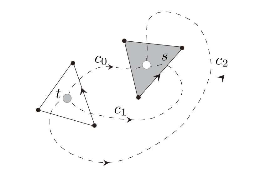
(a) A triconnected pair of tripods

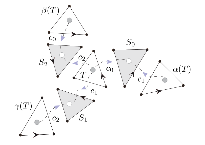
(b) Triconnected tripods in the universal cover

Figure 14. Triconnected tripods and their lifts

Conversely, since $\mathcal{G}/\mathsf{K}_{0}$ is contractible, we may think of a triconnected pair of tripods as a quadruple of tripods $(T,S_{0},S_{1},S_{2})$ in the same connected component of $\mathsf{G}$ well defined up to the diagonal action of $\Gamma$, so that $S_{i}$ all lie in the same $\Gamma$ orbit. In particular, we define an action of $\omega$ on the space of triconnected tripod by

$$\omega(T,S_{0},S_{1},S_{2})\coloneqq(\omega T,\omega^{2}S_{2},\omega^{2}S_{0},\omega^{2}S_{1})\ .$$ (90)

On triconnected pair of tripods the corresponding rotation is

$$\omega(t,s,c_{0},c_{1},c_{2})=(\omega(t),\omega^{2}(s),c_{2},c_{0},c_{1})$$

10.2. Weight functions

We fix a positive $\varepsilon_{0}$ less than half the injectivity radius of $\Gamma\backslash\mathcal{G}$. Let us fix a smooth positive function $\Xi$ from $\mathbb{R}$ to $\mathbb{R}$, with support in $]-1,1[$ and define for every tripod $\tau$ and real $\varepsilon$ the bell function $\Theta_{\tau,x}$ by

$$\Theta_{\tau,\varepsilon}(x)=\frac{1}{\int_{B(\tau,\varepsilon)}\Xi\left(\frac{1}{\varepsilon}d(y,\tau)\right)\ {\rm d}\mu(y)}\Xi\left(\frac{1}{\varepsilon}d(x,\tau)\right)$$

The following proposition is immediate.

Proposition 10.2.1.

The function $\Theta_{\tau,\varepsilon}$ has its support in an $\varepsilon$ neighborhood of $\tau$, is positive and of integral 1. For any isometry $g$ of $\mathcal{G}$,

$$\Theta_{g(\tau),\varepsilon}\circ g=\Theta_{\tau,\varepsilon}\ .$$

Finally, there exists a constant $D$ independent of $\varepsilon$ and $\tau$, so that

$$\|\Theta_{\tau,\varepsilon}\|_{C^{k}}\leqslant D\varepsilon^{-k-D}\ .$$ (91)

Proof.

The technical part is to prove the inequality (91). Let $G_{\lambda}(x)=\Xi\left(\lambda d(x,\tau)\right)$, for $\lambda>1$. An induction shows that for an auxiliary connection $\nabla$ on $\Gamma\backslash\mathcal{G}$ the $k^{\tiny th}$-derivatives of $G_{\lambda}$, $\nabla^{(k)}G_{\lambda}\ ,$ is a polynomial of degree at most $k$ in $\lambda$, the derivatives of $d(x,\tau)$ and the derivatives of $\Xi$, and whose coefficients only depend on $\mathcal{G}/\Gamma$. Since moreover, this polynomial vanishes when $d(x,\tau)>1$, we obtain that

$$\|\nabla^{(k)}G_{\lambda}\|\leqslant K\cdotp\lambda^{k}\ ,$$ (92)

where $K$ only depends on $\Gamma\backslash\mathcal{G}$. Let us also consider the function

$$f(\lambda)=\int_{\Gamma\backslash\mathcal{G}}\Xi\left(\frac{1}{\varepsilon}d(y,\tau)\right)\ {\rm d}\mu(y)=\int_{\Gamma\backslash\mathcal{G}}\Xi\left(\frac{1}{\varepsilon}d(y,\tau)\right){\rm d}\mu(y)\ .$$

Taking a lower bound of the function $\Xi$ be a step function equal to $A$ on the interval $]-C,C[$ and zero elsewhere. Then

$$f(\lambda)\geqslant A\int_{B(\tau,\frac{C}{\lambda})}{\rm d}\mu(y)\geqslant K\left(\frac{1}{\lambda}\right)^{\dim(\mathcal{G})}\ ,$$ (93)

where $K$ only depends on $\mathcal{G}$ and $\Xi$. The proposition now follows at once from inequalities (92) and (93). ∎

As a consequence, the family of functions $\Theta_{\tau,\varepsilon}$ also makes sense on $\Gamma\backslash\mathcal{G}$ and the same property holds: notice that this is the point where we make use of the fact that the lattice is uniform.

Definition 10.2.2.

[Weight Functions] Let $\varepsilon<\varepsilon_{0}$ and $R$ a positive real of absolute value greater than 1. The upstairs weight function is defined on the space of pairs of tripods $(T,S)$ in $\mathcal{G}$ by

$${\rm A}_{\varepsilon,R}(T,S)\coloneqq\int_{\mathcal{G}}\Theta_{T,\frac{\varepsilon}{|R|}}(x)\cdotp\Theta_{S,\frac{\varepsilon}{|R|}}(K\circ\varphi_{R}(x))\,{\rm d}x\ .$$ (94)

The downstairs weight function is defined on the space of pairs of tripods $(t,s)$ in $\Gamma\backslash\mathcal{G}$ by

$${\rm a}_{\varepsilon,R}(t,s):=\int_{\Gamma\backslash\mathcal{G}}\Theta_{t,\frac{\varepsilon}{|R|}}(x)\cdotp\Theta_{s,\frac{\varepsilon}{|R|}}(K\circ\varphi_{R}(x))\,{\rm d}x$$

Let $t$ and $s$ be tripods in $\Gamma\backslash\mathcal{G}$. Let $c_{0}$ be a path from $t$ to $s$. The connected tripod weight function is defined by

$${\rm a}_{\varepsilon,R}(t,s,c_{0}):={{\rm A}}_{\varepsilon,R}(T,S_{0}),$$

where $T$ is any lift of $t$ in $\mathcal{G}$, and $S_{0}$ the lift of $s$ which is the end point of the lift of $c_{0}$ starting at $T$.

Remarks:

1. For $R$ negative, we define

   $${\rm A}_{\varepsilon,R}(T,S)\coloneqq\int_{\mathcal{G}}\Theta_{T,\frac{\varepsilon}{|R|}}(x)\cdotp\Theta_{S,\frac{\varepsilon}{|R|}}(K^{-}\circ\varphi_{R}(x))\,{\rm d}x\ ,$$ (95)

   where $K^{-}(x)=\omega\circ K(x)=\omega^{2}(\bar{x})$. Similarly we define $\rm a_{\varepsilon,R}$.

2. By construction, for any $g\in{\mathsf{G}}$ we have ${\rm A}_{\varepsilon,R}(gT,gS)={\rm A}_{\varepsilon,R}(T,S)$

3. the value of ${\rm a}_{\varepsilon,R}(t,s,c)$ only depends on $t$, $s$ and the homotopy class of $c$.

4. Let $\pi(t,s)$ be the set of homotopy classes of paths from $t$ to $s$, then

   $$\sum_{c\in\pi(t,s)}{\rm a}_{\varepsilon,R}(t,s,c)=\int_{\Gamma\backslash\mathcal{G}}\Theta_{t,\frac{\varepsilon}{|R|}}(x).\Theta_{s,\frac{\varepsilon}{|R|}}(K\circ\varphi_{R}(x)){\rm d}x={{\rm a}}_{\varepsilon,R}(t,s)\,.$$ (96)

Definition 10.2.3.

[Weight of a triconnected pair of tripods] Let $R$ be a positive real. Let $W=(T,S_{0},S_{1},S_{2})$ be a triconnected pair of tripods in the universal cover The weight of $W$ is defined by

$${\rm B}_{\varepsilon,R}(W) = {{\rm A}}_{\varepsilon,R}\left(T,S_{0}\right)\cdotp{{\rm A}}_{\varepsilon,R}\left(\omega^{2}T,\omega S_{1}\right)\cdotp{{\rm A}}_{\varepsilon,R}\left(\omega T,\omega^{2}S_{2}\right)\ .$$ (97)

Similarly, the weight of of a biconnected pair of tripods $B=(T,S_{0},S_{1})$ is defined by

$${\rm D}_{\varepsilon,R}(B)\coloneqq{{\rm A}}_{\varepsilon,R}\left(T,S_{0}\right)\cdotp{\rm A}_{\varepsilon,R}\left(\omega^{2}T,\omega S_{1}\right)\ .$$ (98)

The functions ${\rm B}_{\varepsilon,R}$ and ${\rm D}_{\varepsilon,R}$ are $\Gamma$ invariant and thus descends to functions ${\rm b}_{\varepsilon,R}$ and ${\rm d}_{\varepsilon,R}$ for respectively triconnected tripods and biconnected tripods in $\Gamma\backslash\mathcal{G}$. Using the definition of ${\rm b}_{\varepsilon,R}$ and equation (90)

$${\rm b}_{\varepsilon,R}\circ\omega = {\rm b}_{\varepsilon,R}\ .$$ (99)

$$\sum_{c_{0},c_{1},c_{2}}{\rm b}_{\varepsilon,R}(t,s,c_{0},c_{1},c_{2}) = {\rm a}_{\varepsilon,R}(t,s).{\rm a}_{\varepsilon,R}(\omega^{2}(t),\omega(s)).{\rm a}_{\varepsilon,R}(\omega(t),\omega^{2}(s))\,.$$ (100)

where the last equation used equations (97) and (96),

As an immediate consequence of the definitions of the weight functions we have

Proposition 10.2.4.

Let $(\alpha,\beta,\gamma,\tau_{0},\tau_{1})$ be an $(\frac{\varepsilon}{R},R)$-almost closing pair of pants, let $W\coloneqq(\tau_{0},\tau_{1},\gamma(\tau_{1}),\beta(\tau_{1}))$, Then ${\rm B}_{\varepsilon,R}(W)$ is non zero.

One of our main goal is to prove the converse.

For $R<0$, for reasons that will become clear in Proposition 10.4.3, we define

$${\rm B}_{\varepsilon,R}(W) \coloneqq {{\rm A}}_{\varepsilon,R}(T,\omega^{2}S_{1})\cdotp{{\rm A}}_{\varepsilon,R}(\omega T,\omega S_{0})\cdotp{{\rm A}}_{\varepsilon,R}(\omega^{2}T,S_{2})\ ,$$ (101)

$${\rm D}_{\varepsilon,R}(W) \coloneqq {{\rm A}}_{\varepsilon,R}(T,\omega^{2}S_{1})\cdotp{{\rm A}}_{\varepsilon,R}(\omega T,\omega S_{0})\ .$$ (102)

We have

Proposition 10.2.5.

[Symmetry] We have for $R>0$,

$${\rm A}_{\varepsilon,R}(S,T) = {\rm A}_{\varepsilon,R}(\omega^{2}T,\omega S)$$ (103)

$${\rm D}_{\varepsilon,R}(B) = {\rm A}_{\varepsilon,R}\left(T,S_{0}\right)\cdotp{\rm A}_{\varepsilon,R}\left(S_{1},T\right)\ .$$ (104)

Proof.

By definition, we have

$${\rm A}_{\varepsilon,R}(S,T) = \int_{\mathcal{G}}\Theta_{S,\frac{\varepsilon}{|R|}}(x)\cdotp\Theta_{T,\frac{\varepsilon}{|R|}}(K\circ\varphi_{R}(x))\,{\rm d}x$$ (105)

$$= \int_{\mathcal{G}}\Theta_{S,\frac{\varepsilon}{|R|}}(\varphi_{-R}\circ K^{-1}(x))\cdotp\Theta_{T,\frac{\varepsilon}{|R|}}(x))\,{\rm d}x$$ (106)

$$= \int_{\mathcal{G}}\Theta_{S,\frac{\varepsilon}{|R|}}(\varphi_{-R}(\overline{\omega^{2}(x)}))\cdotp\Theta_{T,\frac{\varepsilon}{|R|}}(x))\,{\rm d}x$$ (107)

$$= \int_{\mathcal{G}}\Theta_{S,\frac{\varepsilon}{|R|}}(\overline{\varphi_{R}\omega^{2}(x)})\cdotp\Theta_{T,\frac{\varepsilon}{|R|}}(x))\,{\rm d}x$$ (108)

$$= \int_{\mathcal{G}}\Theta_{S,\frac{\varepsilon}{|R|}}(\overline{\varphi_{R}(x)})\cdotp\Theta_{T,\frac{\varepsilon}{|R|}}(\omega(x))\,{\rm d}x$$ (109)

$$= \int_{\mathcal{G}}\Theta_{\omega S,\frac{\varepsilon}{|R|}}(K\circ\varphi_{R}(x))\cdotp\Theta_{\omega^{2}T,\frac{\varepsilon}{|R|}}(x)\,{\rm d}x$$ (110)

$$= {\rm A}_{\varepsilon,R}(\omega^{2}T,\omega S).$$ (111)

Where we used the following facts

1. in the first equation, $K$ and $\varphi_{R}$ preserves the volume form,

2. in the second that $K(x)=\omega(\overline{x})$

3. in the third that $\varphi_{R}(\overline{x})=\overline{\varphi_{-R}}$

4. in the fourth the change of variable $y=\omega^{2}(x)$,

5. for the fifth that $\omega$ is an isometry.

The second equation in the proposition is an immediate consequence of the first. ∎

10.2.1. Weight functions and mixing

Recall that a flow $\{\varphi_{t}\}_{t\in\mathbb{R}}$ is exponential mixing if there exists some integer $k$, positive constants $C$ and $a$ so that given two smooth $C^{k}$ functions $f$ and $g$, then for all positive $t$,

$$\left|\int_{X}f.g\circ\varphi_{t}\ {\rm d}\mu-\int_{X}f\ {\rm d}\mu.\int_{X}g\ {\rm d}\mu\right|\leqslant Ce^{-at}\|f\|_{C^{k}}\cdotp\|g\|_{C^{k}}.$$ (112)

In the Appendix 19, we recall the fact that the action of $\{\varphi_{t}\}_{t\in\mathbb{R}}$ on $\Gamma\backslash\mathcal{G}$ is exponentially mixing when $\Gamma$ is a lattice. As an immediate corollary:

Proposition 10.2.6.

[Weight function and mixing] Assume $\Gamma$ is a uniform lattice, there exists a positive constant $q=q(\Gamma)$ depending only on $\Gamma$, a positive constant $K=K(\varepsilon,\Gamma)$ only depending on $\varepsilon$ and $\Gamma$ so that, for $R$ large enough and every $t$, $s$ in $\Gamma\backslash\mathcal{G}$, we have

$$|{\rm a}_{\varepsilon,R}(t,s)-1|\leqslant\exp(-q|R|)\cdotp K.$$ (113)

Proof.

This follows from the definition of exponential mixing and the definition of the function ${\rm a}_{\varepsilon,R}$ by equation (96) and equation (91). ∎

Here is an easy corollary

Corollary 10.2.7.

For any positive $\varepsilon$ then for $R$ large enough, the function ${\rm a}_{\varepsilon,R}$ never vanishes. Moreover, given any $t$ and $s$, there exists $(c_{0},c_{1},c_{2})$ so that ${\rm b}_{\varepsilon,R}(t,s,c_{0},c_{1},c_{2})$ is not zero.

Proof.

The first part follows from the previous proposition (10.2.6), the second part from equation (100). ∎

10.3. Triconnected pair of tripods and almost closing pair of pants

The main theorem of this section is to relate triconnected tripods to a almost closing pair of pants and to prove the converse of Proposition 10.2.4

Theorem 10.3.1.

[Closing up tripods] There exists a constant ${{\bf M}}$ only depending on $\mathsf{G}$, so that the following holds. For any $\varepsilon>0$, there exists $R_{0}$ so that for any triconnected pair of of tripods $W=(T,S_{0},S_{1},S_{2})$ with boundary loops $\alpha$, $\beta$, and $\gamma$, so that ${\rm B}_{\varepsilon,R}(W)\not=0$ with $R>R_{0}$, then $(\alpha,\beta,\gamma,T,S_{0})$ is an $({{\bf M}}\frac{\varepsilon}{R},R)$–positively almost closing pair of pants.

The proof of Theorem 10.3.1 is an immediate consequence of the following proposition.

Proposition 10.3.2.

For $\mu$ small enough and then $R$ large enough. Assuming $B=(T,S_{0},S_{1})$ is a biconnected tripod with boundary loop $\alpha$ so that that ${{\rm D}}_{\mu,R}(B)\not=0$. Then $T$ and $S_{0}$ are $(\frac{\mu}{R},R)$-almost closing for $\alpha$.

Proof.

We have $S_{0}=\alpha(S_{1})$. Since ${\rm{\rm A}}_{R,\mu}(T,S_{0})\not=0$, there exists $u$ so that

$$\Theta_{T,\frac{\mu}{R}}(u).\Theta_{S_{0},\frac{\mu}{R}}(K\circ\varphi_{R}(u))\not=0.$$

Thus, from the definition of $\Theta$,

$$d(u,T)\leqslant\frac{\mu}{R}\ ,\ \ d(K\circ\varphi_{R}(u),S_{0})\leqslant\frac{\mu}{R}.$$ (114)

Similarly, since ${\rm{\rm A}}_{R,\mu}(\omega^{2}(T),\omega(S_{1}))\not=0$, there exists a tripod $z$ so that

$$d(\omega(z),T)\leqslant d(z,\omega^{2}(T))\leqslant\frac{\mu}{R} d(K\circ\varphi_{R}(z),\omega(S_{1}))\leqslant\frac{\mu}{R}\ .$$ , (115)

here we used that $\omega$ is an isometry for $d$ (see beginning of paragraph 3.4). Let

$$v\coloneqq\alpha(\omega^{2}\circ K\circ\varphi_{R}(z))=\alpha(\overline{\varphi_{R}(z)}).$$

Then using the fact the metric on $\mathcal{G}$ is invariant by ${\mathsf{G}}$ and $\omega$ and using Corollary 3.4.5

$$d(v,S_{0})=d(v,\alpha(S_{1}))=d(\omega^{2}\circ K\circ\varphi_{R}(z),S_{1})=d(K\circ\varphi_{R}(z),\omega(S_{1}))\leqslant\frac{\mu}{R},$$ (116)

Moreover, using the commutations properties (3.3.1), we have

$$K\circ\varphi_{R}(v)=\omega(\overline{\varphi_{R}(\alpha(\overline{\varphi_{R}(z)})})=\alpha\circ\omega(\varphi_{-R}(\varphi_{R}(z)))=\alpha(\omega(z)).$$

Thus, first inequality (115) and combining with inequality (116)

$$d(K\circ\varphi_{R}(v),\alpha(T))\leqslant\frac{\mu}{R} d(v,S_{0})\leqslant\frac{\mu}{R}\ \ .$$ , (117)

The result now follows from inequality (117) and (114). ∎

10.4. Reversing orientation on triconnected and biconnected pair of tripods

We need an analogue of the transformation that reverse the orientation on pair of pants. Let ${{\bf J}}_{0}$ in $\operatorname{Aut}(\mathsf{G}_{0})$ be a reflexion for $\mathfrak{s}_{0}$ (see 2.1). Let $\sigma$ be the involution $x\mapsto\overline{x}$ defined in paragraph 3.3. For an even $\mathfrak{sl}_{2}$-triple, ${{\bf J}}_{0}$ and $\sigma$ commute: this follows from a direct matrix computation. Recall also that the automorphism ${{\bf J}}_{0}$ fixes $\mathsf{L}_{0}$ pointwise since by definition ${{\bf J}}_{0}\in\mathsf{Z}(\mathsf{L}_{0})$.

Definition 10.4.1.

[Reverting orientation on $\mathcal{G}$] The reverting orientation involution ${{\bf I}}_{0}$ is the automorphism of $\mathsf{G}_{0}$ defined by ${{\bf I}}_{0}\coloneqq{{\bf J}}_{0}\circ\sigma$.

We use the same notation to define its action on the space of tripods $\mathcal{G}=\operatorname{Hom}(\mathsf{G}_{0},\mathsf{G})$ by precomposition.

Remarks:

1. ${{\bf I}}_{0}$ commutes with $\sigma$, and if $\mathfrak{s}_{0}=(a_{0},x_{0},y_{0})$ is the fundamental ${\mathfrak{sl}_{2}}$-triple, then

   $${{\bf I}}_{0}(a_{0},x_{0},y_{0})=(-a_{0},y_{0},x_{0})\ .$$ (118)

2. we have ${{\bf I}}_{0}\circ\varphi_{R}=\varphi_{-R}\circ{{{\bf I}}}_{0}$, similarly $\omega\circ{{\bf I}}_{0}={{\bf I}}_{0}\circ\omega^{2}$ and ${{\bf I}}_{0}\circ K\circ{{\bf I}}_{0}=\omega\circ K$

3. for any tripod $\tau$, $\delta^{\pm}{{\bf I}}_{0}(\tau)=\delta^{\mp}\tau$ and $\delta^{0}({{\bf I}}_{0}(\tau))=\delta^{0}(\tau)$.

4. Since the action of ${{{\bf I}}_{0}}$ commutes with the action of ${\mathsf{G}}$ and generates together with $\omega$ a finite group, we may assume that it preserves the left invariant metric on $\mathcal{G}$.

5. When ${\mathsf{G}}$ is isomorphic to $\mathsf{PSL}_{2}(\mathbb{C})$, ${{\bf I}}_{0}$ corresponds to the symmetry $J$ with respect to a geodesic.

Definition 10.4.2.

[Reverting orientation and rotation on $\mathcal{Q}$] The reverting involution ${{\bf I}}_{0}$ – see Figure 15 – on the set of triconnected pairs of tripods $\mathcal{Q}$, given by

$${{\bf I}}_{0}(t,s,c_{0},c_{1},c_{2}) \coloneqq ({{\bf I}}_{0}(t),\omega{{\bf I}}_{0}(s)),\omega^{2}{{\bf I}}_{0}(c_{1}),\omega^{2}{{\bf I}}_{0}(c_{0}),\omega^{2}{{\bf I}}_{0}(c_{2}))\ .$$ (119)

On the set $\mathcal{B}$ of biconnected pairs of tripods, it is given by

$${{\bf I}}_{0}(t,s,c_{0},c_{1})\coloneqq({{\bf I}}_{0}(t),\omega{{\bf I}}_{0}(s),\omega^{2}{{\bf I}}_{0}(c_{1}),\omega^{2}{{\bf I}}_{0}(c_{0}))\ .$$ (120)

In order for this definition to make sense, we need to check that ${{\bf I}}_{0}$ sends a triconnected pairs of tripods to a triconnected pairs of tripods

Proof.

Recall that a triconnected pair of tripods is a quintuple $(t,s,c_{0},c_{1},c_{2})$,

• $c_{0}$ goes from $t$ to $s$,

• $c_{1}$ goes from $\omega^{2}t$ to $\omega s$

• $c_{2}$ goes from $\omega t$ to $\omega^{2}s$

Let us check that $({{\bf I}}_{0}(t),\omega{{\bf I}}_{0}(s)),\omega^{2}{{\bf I}}_{0}(c_{1}),\omega^{2}{{\bf I}}_{0}(c_{0}),\omega{{\bf I}}_{0}(c_{2}))$ is a triconnected pair of tripods. Indeed, denoting $u={{\bf I}}_{0}(t)$ and $v=\omega{{\bf I}}_{0}(s)$, we have

1. $\omega^{2}{{\bf I}}_{0}(c_{1})$ goes from $\omega^{2}{{\bf I}}_{0}\omega^{2}(t)={{\bf I}}_{0}(t)=u$ to $\omega^{2}{{\bf I}}_{0}\omega(s)=\omega{{\bf I}}_{0}(s)=v$,

2. $\omega^{2}{{\bf I}}_{0}(c_{0})$ goes from $\omega^{2}{{\bf I}}_{0}(t)=\omega^{2}(u)$ to $\omega^{2}{{\bf I}}_{0}(s)=\omega(v)$,

3. $\omega^{2}{{\bf I}}_{0}(c_{2})$ goes from $\omega^{2}{{\bf I}}_{0}\omega(t)=\omega{{\bf I}}_{0}(t)=\omega(u)$ to $\omega^{2}{{\bf I}}_{0}\omega^{2}(s)={{\bf I}}_{0}(s)=\omega^{2}(v)$,

Thus, indeed, ${{\bf I}}_{0}$ sends triconnected pairs of tripods to triconnected pairs of tripods. ∎

(a) Before

(b) After

Figure 15. Reverting orientation on triconnected tripods: here ${{\bf I}}=\omega{{\bf I}}_{0}$.

Reverting orientation plays well with the weight functions and boundary loops:

Proposition 10.4.3.

Let $q=(t,s,c_{0},c_{1},c_{2})$ be a triconnected pair of tripods

1. If the lift of $q$ is $W=(T,S_{0},S_{1},S_{2})$ then the lift of ${{\bf I}}_{0}(q)$ is

   $${{\bf I}}_{0}(W)\coloneqq\left({{\bf I}}_{0}(T),\omega{{\bf I}}_{0}(S_{1}),\omega{{\bf I}}_{0}(S_{0}),\omega{{\bf I}}_{0}(S_{2})\right)$$

2. If the boundary loops of $q$ are $(\alpha,\beta,\gamma)$ then those of ${{\bf I}}_{0}(q)$ are $(\alpha^{-1},\gamma^{-1},\beta^{-1})$. In particular ${{\bf I}}_{0}$ sends $\mathcal{Q}_{[\alpha]}$ to $\mathcal{Q}_{[\alpha^{-1}]}$.

3. Finally,

   $${{\bf I}}_{0}\circ\omega=\omega^{2}\circ{{\bf I}}_{0}\ \ ,\ \ {\rm b}_{\varepsilon,R}\circ{{\bf I}}_{0}={\rm b}_{\varepsilon,-R} {\rm d}_{\varepsilon,R}\circ{{\bf I}}_{0}={\rm d}_{\varepsilon,-R}\ .$$ , (121)

Proof.

This follows either from squinting at symmetries in Figure (15) or from tedious computations that we officiate now.

For the first item, observe that

• the lift of $\omega^{2}{{\bf I}}_{0}(c_{1})$ goes from $\omega^{2}{{\bf I}}_{0}\omega^{2}(T)={{\bf I}}_{0}(T)$ to $\omega^{2}{{\bf I}}_{0}\omega(S_{1})=\omega{{\bf I}}_{0}(S_{1})$,

• the lift of $\omega^{2}{{\bf I}}_{0}(c_{0})$ goes from $\omega^{2}{{\bf I}}_{0}(T)$ to $\omega^{2}{{\bf I}}_{0}(S_{0})=\omega\left(\omega{{\bf I}}_{0}(S_{0})\right)$,

• the lift of $\omega^{2}{{\bf I}}_{0}(c_{2})$ goes from $\omega^{2}{{\bf I}}_{0}\omega(T)={{\bf I}}_{0}(T)$ to $\omega^{2}{{\bf I}}_{0}\omega^{2}(S_{2})=\omega^{2}\left(\omega{{\bf I}}_{0}(S_{2})\right)$.

The second item now follows from the first and the fact that $\Gamma$ commutes with ${{\bf I}}_{0}$ and $\omega$.

Let us now check the third item. For the sake of convenience, we use the abusive notation $\Theta_{t,\frac{\varepsilon}{|R|}}=\Theta_{t}$. Thus for $R>0$,

$${\rm A}_{\varepsilon,R}({{\bf I}}_{0}(T),{{\bf I}}_{0}(S)) = \int_{\mathcal{G}}\Theta_{{{\bf I}}_{0}(T)}(x)\cdot\Theta_{{{\bf I}}_{0}(S)}(K\circ\varphi_{R}(x))\,{\rm d}x$$

$$= \int_{\mathcal{G}}\Theta_{T}({{\bf I}}_{0}(x))\cdotp\Theta_{S}({{\bf I}}_{0}\circ K\circ\varphi_{R}(x))\,{\rm d}x$$

$$= \int_{\mathcal{G}}\Theta_{T}(x)\cdotp\Theta_{S}({{\bf I}}_{0}\circ K\circ\varphi_{R}\circ{{\bf I}}_{0}(x))\,{\rm d}x$$

$$= \int_{\mathcal{G}}\Theta_{T}(x)\cdotp\Theta_{S}(\omega\circ K\circ\varphi_{-R}(x))\,{\rm d}x$$

$$= {\rm A}_{\varepsilon,-R}(T,S)\ ,$$

where for equation (10.4) we used the equivariance of $\Theta$, for equation (10.4) a change of variables in $\mathcal{G}$ and in equation (10.4) the commuting relations ((ii)) following definition 10.4.2. Let $q=(t,s,c_{0},c_{1},c_{2})$ with lift $W=(T,S_{0},S_{1},S_{2})$. Recall that

$${{\rm B}}_{\varepsilon,R}(W) = {\rm A}_{\varepsilon,R}(T,S_{0}).{\rm A}_{\varepsilon,R}(\omega^{2}T,\omega S_{1}).{\rm A}_{\varepsilon,R}(\omega T,\omega^{2}S_{2})\ ,$$

$${\rm B}_{\varepsilon-R}(W) = {\rm A}_{\varepsilon,R}(\omega T,\omega S_{0}).{\rm A}_{\varepsilon,R}(T,\omega^{2}S_{1}).{\rm A}_{\varepsilon,R}(\omega^{2}T,S_{2})\ .$$

Thus

$${\rm b}_{\varepsilon,R}({{\bf I}}_{0}(W)) = {{\rm A}}_{\varepsilon,R}({{\bf I}}_{0}(T),\omega{{\bf I}}_{0}(S_{1})\cdotp{{\rm A}}_{\varepsilon,R}(\omega^{2}{{\bf I}}_{0}(T),\omega^{2}{{\bf I}}_{0}(S_{0}))\cdotp{{\rm A}}_{\varepsilon,R}(\omega{{\bf I}}_{0}(T),{{\bf I}}_{0}(S_{2}))$$

$$= {{\rm A}}_{\varepsilon,R}({{\bf I}}_{0}(T),{{\bf I}}_{0}(\omega^{2}S_{1}))\cdotp{{\rm A}}_{\varepsilon,R}({{\bf I}}_{0}(\omega T),{{\bf I}}_{0}(\omega S_{0}))\cdotp{{\rm A}}_{\varepsilon,R}({{\bf I}}_{0}(\omega^{2}T),{{\bf I}}_{0}(S_{2}))$$

$$= {{\rm A}}_{\varepsilon,-R}(T,\omega^{2}S_{1})\cdotp{{\rm A}}_{\varepsilon,-R}(\omega T,\omega S_{0})\cdotp{{\rm A}}_{\varepsilon,R}(\omega^{2}T,S_{2})$$

$$= {{\rm B}}_{\varepsilon,-R}(T,S_{0},S_{1},S_{2})$$

$$= {\rm b}_{\varepsilon,-R}(q)\ .$$

The commutations properties between $\omega$ and ${{\bf I}}_{0}$ are straightforward. And the relations for $\rm d_{\varepsilon,R}$ are obtained in the same way. ∎

10.5. Definition of negatively almost closing pair of pants

Assume $\varepsilon$ and $R$ are positive constants. If $p=(\alpha,\beta,\gamma,\tau_{0},\tau_{1})$ is an $(\varepsilon,R)$- (positively) almost closing pair of pants. Then by definition

$${{\bf I}}_{0}(p)\coloneqq(\alpha^{-1},\gamma^{-1},\beta^{-1},{{\bf I}}_{0}(\tau_{0}),\omega{{\bf I}}_{0}(\tau_{1}))$$

is an $(\varepsilon,-R)$- (negatively)-almost closing pair of pants.

Then Theorem 10.3.1 holds for $R<0$, as an immediate symmetry consequence of the properties of ${{\bf I}}_{0}$.

11. Spaces of biconnected tripods and triconnected tripods

We present in this section the spaces of biconnected and triconnected tripods that we shall discuss in the next sections. Our goal in this section are

1. The definition of the various spaces involved

2. The Equidistribution and Mixing Proposition 11.3.1

3. Some local connectedness properties of the space of almost closing pair of pants.

Throughout this section, $\Gamma$ will be a uniform lattice in $\mathsf{G}$. Let $\alpha\in\Gamma$ be a $\mathsf{P}$-loxodromic element. Recall that (see for instance [11, Proposition 3.5]) the centralizer

$$\Gamma_{\alpha}\coloneqq\mathsf{Z}_{\Gamma}(\alpha),$$

of $\alpha$ in $\Gamma$ is a uniform lattice in the centralizer $\mathsf{Z}_{\mathsf{G}}(\alpha)$ of $\alpha$ in $\mathsf{G}$.

11.1. Biconnected tripods

Let $\alpha$ be a $\mathsf{P}$-loxodromic element and $\Lambda$ be a uniform lattice in $\mathsf{Z}_{\mathsf{G}}(\alpha)$. We define the upstairs space of biconnected tripods $\mathcal{B}_{\alpha}$ as

$$\mathcal{B}_{\alpha}\coloneqq\{(T,S_{0},S_{1})\hbox{ biconnected tripods in the universal cover}\mid S_{0}=\alpha S_{1}\}$$

and the downstairs space of biconnected tripods as

$$\mathcal{B}^{\Lambda}_{\alpha}\coloneqq\Lambda\backslash\mathcal{B}_{\alpha}\ .$$

We shall also denote by $[\Gamma]$ be the set of conjugacy classes of elements in $\Gamma$, that we also interpret as the set of free homotopy classes in $\Gamma\backslash\mathsf{G}/\mathsf{K}_{0}$, where $K_{0}$ is the maximal compact of $\mathsf{G}_{0}$.

11.1.1. An invariant measure

Observe that $\mathcal{B}_{\alpha}$ can be identified with $(\mathcal{G}\times\mathcal{G})^{*}$ (that is the space of pairs of tripods in the same connected component). From the covering map from $\mathcal{B}^{\Lambda}_{\alpha}$ to $\Lambda\backslash\mathsf{G}\times\Lambda\backslash\mathsf{G}$, we deduce a invariant form $\lambda$ in the Lebesgue measure class of $\mathcal{B}_{\alpha}$ and $\mathcal{B}^{\Lambda}_{\alpha}$.

Let also ${\rm D}_{\varepsilon,R}$ and ${\rm d}_{\varepsilon,R}$ the weight functions defined in Definition 10.2.3 (with respect to $\Gamma=\Lambda$) By construction ${\rm D}_{\varepsilon,R}$ is a function on $\mathcal{B}_{\alpha}$, while ${\rm d}_{\varepsilon,R}$ is a function on $\mathcal{B}^{\Lambda}_{\alpha}$. We now consider the measures

$$\tilde{\nu}_{\varepsilon,R}={\rm D}_{\varepsilon,R}\cdotp\lambda\ ,\ \nu_{\varepsilon,R}={\rm d}_{\varepsilon,R}\cdotp\lambda\ ,$$

on $\mathcal{B}^{u}_{\alpha}$ and $\mathcal{B}^{\Lambda}_{\alpha}$ respectively. The following are obvious

Proposition 11.1.1.

The measure $\nu_{\varepsilon,R}$ is locally finite and invariant under $\mathsf{C}_{\alpha}\coloneqq{\bf Z}^{\circ}_{\mathsf{G}}(\Lambda)$.

We finally consider $\mathcal{B}_{\varepsilon,R}(\alpha)$ and $\mathcal{B}^{\Lambda}_{\varepsilon,R}(\alpha)$ the supports of the functions ${\rm D}_{\varepsilon,R}$ and ${\rm d}_{\varepsilon,R}$. It will be convenient in the sequel to distinguish between positive and negative and we introduce for $R>0$,

$$\mathcal{B}^{+}_{\varepsilon,R}(\alpha)=\{B\in\mathcal{B}_{\alpha}\mid{\rm D}_{\varepsilon,R}(B)>0\} \mathcal{B}^{\Lambda,+}_{\varepsilon,R}(\alpha)=\{B\in\mathcal{B}^{\Lambda}_{\alpha}\mid{\rm d}_{\varepsilon,R}(B)>0\}\ ,$$ ,

$$\mathcal{B}^{-}_{\varepsilon,R}(\alpha)=\{B\in\mathcal{B}_{\alpha}\mid{\rm D}_{\varepsilon,-R}(B)>0\} \mathcal{B}^{\Lambda,-}_{\varepsilon,R}(\alpha)=\{B\in\mathcal{B}^{\Lambda}_{\alpha}\mid{\rm d}_{\varepsilon,-R}(B)>0\}\ .$$ ,

Recall that by Proposition 10.3.2, if $(T,S_{0},\alpha(S_{0}))$ belong to $\mathcal{B}_{\varepsilon,R}(\alpha)$, then $T$ and $S_{0}$ are $(\frac{\varepsilon}{R},R)$-almost closing for $\alpha$.

11.1.2. Biconnected tripods and lattices

Let $\Gamma$ be a uniform lattice in $\mathsf{G}$ and $\alpha$ a $\mathsf{P}$-loxodromic element in $\Gamma$. We may now consider the set of biconnected tripods in $\Gamma\backslash\mathsf{G}$ whose loop is in the homotopy class defined by $\alpha$.

$$\mathcal{B}^{\Gamma}_{[\alpha]}\coloneqq\{(t,s,c_{0},c_{1})\hbox{ biconnected tripods in }\Gamma\backslash\mathsf{G}\mid c_{0}\bullet c_{1}^{-1}\in[\alpha]\}$$

We have the following interpretation.

Proposition 11.1.2.

The projection from $\mathcal{B}^{\Gamma_{\alpha}}_{\alpha}$ to $\mathcal{B}^{\Gamma}_{[\alpha]}$ is an isomorphism.

In the sequel we will use the following abuse of language: $\mathcal{B}^{\Gamma}_{\alpha}\coloneqq\mathcal{B}^{\Gamma_{\alpha}}_{\alpha}$.

11.2. Triconnected tripods

We need to give names to various spaces of triconnected tripods, including their “boundary related” versions. Let as above $\Gamma$ be a uniform lattice, $\alpha$ be an element in $\Gamma$ and $\Lambda$ a lattice in $\mathsf{Z}_{\mathsf{G}}(\alpha)$. We introduce the following spaces

$$\mathcal{Q} \coloneqq \{(T,S_{0},S_{1},S_{2})\in\mathcal{G}^{4}\mid S_{1},S_{2}\in\Gamma\cdotp S_{0}\}\ ,$$

$$\mathcal{Q}^{\Gamma} \coloneqq \{(t,s,c_{0},c_{1},c_{2})\hbox{ triconnected tripods in }\Gamma\backslash\mathsf{G}\}\ ,$$

$$\mathcal{Q}_{\alpha} \coloneqq \{(T,S_{0},S_{1},S_{2})\in\mathcal{Q}\mid S_{1}=\alpha S_{0}\}\ ,$$

$$\mathcal{Q}^{\Lambda}_{\alpha} \coloneqq \Lambda\backslash\mathcal{Q}_{\alpha}\ ,$$

$$\mathcal{Q}^{\Gamma}_{[\alpha]} \coloneqq \{(t,s,c_{0},c_{1},c_{2})\in\mathcal{Q}^{\Gamma}\mid c_{0}\bullet c_{1}^{-1}\in[\alpha]\}\ .$$

The following identifications are obvious

Proposition 11.2.1.

We have that $\mathcal{Q}^{\Gamma}$ is isomorphic to $\Gamma\backslash\mathcal{Q}$. Similarly $\mathcal{Q}^{\Gamma}_{[\alpha]}$ is isomorphic to $\mathcal{Q}^{\Gamma_{\alpha}}_{\alpha}$. Finally

$$\mathcal{Q}^{\Gamma}=\bigsqcup_{[\alpha]\in[\Gamma]}\mathcal{Q}^{\Gamma}_{[\alpha]}.$$

By a slight abuse of language we shall write $\mathcal{Q}^{\Gamma}_{\alpha}\coloneqq\mathcal{Q}^{\Gamma_{\alpha}}_{\alpha}$.

11.2.1. Triconnected tripods in $\Gamma\backslash\mathsf{G}$

Parallel to what we did for biconnected tripods, let us introduce the following spaces. First Let $\mathcal{Q}^{\Gamma}$ be the set of triconnected pairs of tripods in $\Gamma\backslash\mathcal{G}$ and let

$$\mathcal{Q}^{\Gamma}_{\varepsilon,R}=\{w\in\mathcal{Q}^{\Gamma}\mid{\rm b}_{\varepsilon,R}(w)>0\}.$$

We will assume $R>0$ and write accordingly $\mathcal{Q}^{\Gamma,+}_{\varepsilon,R}=\mathcal{Q}^{\Gamma}_{\varepsilon,R}$ and $\mathcal{Q}^{\Gamma,-}_{\varepsilon,R}=\mathcal{Q}^{\Gamma}_{\varepsilon,-R}$. Let $(\Gamma\backslash\mathcal{G}\times\Gamma\backslash\mathcal{G})^{*}$ be the set of pairs of points in $\Gamma\backslash\mathcal{G}$ in the same connected component. We first observe

Proposition 11.2.2.

The (forgetting) map $p$ from $\mathcal{Q}^{\Gamma}$ to $(\Gamma\backslash\mathcal{G}\times\Gamma\backslash\mathcal{G})^{*}$ sending $(t,s,c_{0},c_{1},c_{2})$ to $t,s)$ is a covering.

Proof.

Let ${\mathcal{Q}}_{u}$ be the space of quadruples $(T,S_{0},S_{1},S_{2})$ where all $S_{i}$ lie in the same $\Gamma$ orbit. The map $\pi:(T,S_{0},S_{1},S_{2})\mapsto(T,S_{0})$ is a covering. Let $\Gamma\times\Gamma$ be acting on ${\mathcal{Q}}_{u}$ by $(\gamma,\eta)\cdotp(T,S_{0},S_{1},S_{2})=(\gamma T,\eta S_{0},\eta S_{1},\eta S_{2})$. Then $(\Gamma\times\Gamma)\backslash{\mathcal{Q}}_{u}=\mathcal{Q}$ and $\pi$ being equivariant gives rise to $p$. Thus $p$ is a covering. ∎

Definition 11.2.3.

[Measures] The Lebesgue measure $\Lambda$ is the locally finite measure on $\mathcal{Q}$ associated to the pullback of the $\mathsf{G}$-invariant volume form on $\Gamma\backslash\mathcal{G}$.

Given positive $R$ and $\varepsilon$, the weighted measure $\mu_{\varepsilon,R}$ on $\mathcal{Q}$ is the measure supported on $\mathcal{Q}_{\varepsilon,R}$ given by $\mu_{\varepsilon,R}\coloneqq{\rm b}_{\varepsilon,R}\Lambda$.

For the sake of convenience, we will assume that $R>0$ and write $\mu^{+}_{\varepsilon,R}\coloneqq\mu_{\varepsilon,R}$ and $\mu^{-}_{\varepsilon,R}\coloneqq\mu_{\varepsilon,-R}$

Proposition 11.2.4.

For any positive $\varepsilon$, then $R$ large enough, $\mathcal{Q}^{\Gamma}_{\varepsilon,R}$ is non empty, relatively compact and $\mu_{\varepsilon,R}$ is finite. Moreover

$$\omega_{*}\mu^{\pm}_{\varepsilon,R}=\mu^{\pm}_{\varepsilon,R}\ \ ,\ \ {{{\bf I}}_{0}}_{*}\mu^{\pm}_{\varepsilon,R}=\mu^{\mp}_{\varepsilon,R}\ .$$

Proof.

By Corollary 10.2.7, ${\rm b}_{\varepsilon,R}$ is not always zero, thus $\mathcal{Q}^{\Gamma}_{\varepsilon,R}$ is non empty. Let $(T,S_{0},S_{1},S_{2})$ be a lift of a triconnected tripod $w=(t,s,c_{0},c_{1},c_{2})$ satisfying ${\rm b}_{\varepsilon,R}(w)\not=0$. Then, by Proposition 10.3.2, $d(T,S_{i})\leqslant R+\varepsilon$. This implies that $\mathcal{Q}_{\varepsilon,R}$ is relatively compact and thus $\mu_{\varepsilon,R}$ is finite. The invariance by $\omega$ comes from the invariance of ${\rm b}_{\varepsilon,R}$ by $\omega$ (Equation (99)) and the invariance of the metric by $\omega$. The last assertion comes from the fact that ${\rm b}_{\varepsilon,R}={\rm b}_{\varepsilon,-R}\circ I$ by Proposition 10.4.3 and that $\Lambda$ is invariant by $I$, since the invariant measure on $\mathcal{G}$ is invariant by $\operatorname{Aut}(\mathsf{G}_{0})$ (see beginning of paragraph 3.4). ∎

Let’s finally define $\mathcal{Q}^{\Gamma}_{\varepsilon,R}(\alpha)\coloneqq\mathcal{Q}^{\Gamma}_{\varepsilon,R}\cap\mathcal{Q}^{\Gamma}_{\alpha}$.

11.3. Mixing: From triconnected tripods to biconnected tripods

We have a natural forgetful map $\pi$ from $\mathcal{Q}^{\Gamma}_{\alpha}$ to $\mathcal{B}^{\Gamma}_{\alpha}$: $\pi(T,S_{0},S_{1},S_{2})\coloneqq(T,S_{0},S_{1})$. We then have the following proposition which says that adding a third path is probabilistically independent for large $R$.

Proposition 11.3.1.

[Equidistribution and mixing] We have the inclusion $\pi(\mathcal{Q}_{\varepsilon,R}(\alpha))\subset\mathcal{B}_{\varepsilon,R}(\alpha)$. Moreover, there exists a function $C_{\varepsilon,R}$ depending on $R$ and $\varepsilon$, a constant $q$ and a constant $K(\varepsilon,\Gamma)$ so that $\pi_{*}\left(\mu_{\varepsilon,R}\right)=C_{\varepsilon,R}\cdotp\nu_{\varepsilon,R}$. The function ${\rm C}_{\varepsilon,R}$ is a smooth almost constant function: there exists a constant $q$ and a constant $K(\varepsilon,\Gamma)$ so that

$$\left\|{\rm C_{\varepsilon,R}}-1\right\|_{C^{0}}\leqslant K(\varepsilon,\Gamma)\exp(-q|R|)\ .$$ (122)

In particular, given $\varepsilon$, for $R$ large enough, the measure $\nu_{\varepsilon,R}$ is finite with relatively compact support.

Proof.

By construction for the second equality, and assertion (96) for the third

$$\pi_{*}\left({\mu}_{\varepsilon,R}\right)=\pi_{*}\left({\rm b}_{\varepsilon,R}\Lambda\right)=\left(\sum_{c_{2}}{\rm a}_{\varepsilon,R}(\omega(t),\omega^{2}(s),c_{2})\right)\cdotp{\rm d}_{\varepsilon,R}\Lambda=a_{\varepsilon,R}(\omega(t),\omega^{2}(s))\Lambda\ .$$

Thus the result follows from exponential mixing: Proposition 10.2.6 and taking

$${\rm C}_{\varepsilon,R}(t,s)\coloneqq\sum_{c_{2}}{\rm a}_{\varepsilon,R}(\omega(t),\omega^{2}(s),c_{2})\ =a_{\varepsilon,R}(\omega(t),\omega^{2}(s).$$

Observe that ${\rm C}_{\varepsilon,R}$ is smooth since only finitely many terms in the sum are non zero: there are only finitely many homotopy classes of arcs of bounded length. ∎

11.4. Perfecting pants and varying the boundary holonomies

By a slight abuse of language we will say that $(T,S_{0},S_{1},S_{2})$ with boundary loops $(\alpha,\beta,\gamma)$ is $(\frac{\varepsilon}{R},R)$-almost closing if $(\alpha,\beta,\gamma,T,S_{0})$, where $S_{2}=\beta(\omega^{2}S_{0})$ and $S_{0}=\alpha(\omega^{2}S_{1})$ is $(\frac{\varepsilon}{R},R)$-almost closing.

Let us denote by $P_{\varepsilon,R}$ the space of $(\varepsilon,R)$-almost closing pair of pants.

We say a boundary loop of a triconnected pair of pants is $T$-perfect if it is conjugate to $\exp(2Ta)$. Given $R$, recall that the boundary loops of an $R$-perfect pair of pants are $R$-perfect (See [21, Proposition 5.2.2]).

Recall that if $\alpha$ is a $\mathsf{P}$-loxodromic element, we denote by $\mathsf{L}_{\alpha}$ the stabilizer in $\mathsf{G}$ of the attractive and repulsive points $\alpha^{+}$ and $\alpha^{-}$.

Our main result is the following

Theorem 11.4.1.

[Varying the boundary holonomies] Let $B$ be a positive number. Then there exists positive constants $\varepsilon_{0}$ and $C$, so that given $\varepsilon<\varepsilon_{0}$, then for $R$ large enough the following assertion holds:

Let $W_{0}=(T,S_{0},S_{1},S_{2})$ be a pair of pants in $P_{\varepsilon,R}$ with boundary loops $\alpha_{0}$, $\beta_{0}$ and $\gamma_{0}$.

Let $\{k_{t}\}_{t\in[0,1]}$ be a smooth path in $\mathsf{L}_{\alpha_{0}}$ in the ball of radius of length less than $B\frac{\varepsilon}{R}$ with respect to $d_{T}$.

Then there exists a a continuous family $\{W_{t}\}_{t\in[0,1]}$ in $P_{C\varepsilon,R}$ with boundary loops $\alpha_{t}$, $\beta_{t}$, $\gamma_{t}$ so that $W_{0}=W$ and

1. for all $t$, $\beta_{t}$ and $\gamma_{t}$ are conjugate to $\beta_{0}$ and $\gamma_{0}$ respectively,

2. $\alpha_{t}$ is conjugate to $\alpha_{0}\cdotp k_{t}$.

11.4.1. Lifting holonomies

Let $W=(T,S_{0},S_{1},S_{2})$. For any $h$ in $\mathsf{G}$ let

$$W_{h}=(T,S_{0},hS_{1},S_{2})\ .$$

Observe that if $h$ belongs to the ball of radius $\frac{\varepsilon}{R}$ with respect to $d_{T}$ then $W$ is $(M\frac{\varepsilon}{R},R)$ almost closing for some uniform $M$.

The boundary loops of $W_{h}$ are now $\alpha_{h}\coloneqq\alpha\cdotp h^{-1}$, $\beta_{h}=\beta$ and $\gamma_{h}\coloneqq h\cdotp\gamma$.

Let $\mathsf{G}_{\varepsilon,R}$, respectively $\mathsf{L}_{\varepsilon,R}$, the ball of radius $\frac{\varepsilon}{R}$ in $\mathsf{G}$, respectively $\mathsf{L}_{0}$.

Let us consider, for this section,

1. the map $A$ from the ball $\mathsf{G}_{\varepsilon,R}$ of radius $\frac{\varepsilon}{R}$ in $\mathsf{G}$ to the ball $\mathsf{L}_{M\varepsilon,R}$ so that $\alpha_{h}$ is conjugate to $\exp(Ra_{0})\cdotp A(h)$.

2. Similarly let $C$ the map from $\mathsf{G}_{\varepsilon,R}$ to $\mathsf{L}_{M\varepsilon,R}$ so that $\gamma_{h}$ is conjugate to $\exp(Ra_{0})\cdotp C(h)$.

For $\varepsilon$ small enough and $M$ large enough, so these maps are well defined by the Boundary Loop proposition.

We need a succession of technical result

Lemma 11.4.2.

[Horizontal distribution] There exists constant $K_{0}$ and $\varepsilon_{0}$ so that for $\varepsilon$ less than $\varepsilon_{0}$ For any $h$ in $\mathsf{G}_{\varepsilon,R}$, there exists a linear subspace $H_{h}$ in $\mathsf{T}_{h}\mathsf{G}$, depending smoothly on $h$, so that

1. $\mathsf{T}_{h}C$ is zero restricted to $H_{h}$

2. $\mathsf{T}_{h}A$ is uniformly $K_{0}$ bilipschitz from $H_{h}$ to $T_{A(h)}\mathsf{L}_{0}$.

We will refer to $H$ as the horizontal distribution.

Proof.

Let us linearize the problem. Given a deformation $\{k_{t}\}_{t\in[0,1]}$, we are looking for $\{h_{t}\}_{t\in[0,1]}$, $\{f_{t}\}_{t\in[0,1]}$ and $\{g_{t}\}_{t\in[0,1]}$ so that

$$\alpha\cdotp h_{t}^{-1}=f_{t}\cdotp\alpha\cdotp k_{t}\cdotp f_{t}^{-1}\ \ ,\ \ h_{t}\cdotp\gamma=g_{t}\cdotp\gamma\cdotp g_{t}^{-1}\ .$$

Writing $\accentset{\mbox{\large.}}{v}=\left.\frac{{\rm d}v}{{\rm d}t}\right|\mid_{t=0}$, we get the linearized equation

$$\accentset{\mbox{\large.}}{h}=(\operatorname{Ad}(\alpha)-1)\cdotp\accentset{\mbox{\large.}}{f}+\accentset{\mbox{\large.}}{k}\ \ ,\ \ \accentset{\mbox{\large.}}{h}=(1-\operatorname{Ad}(\gamma))\cdotp\accentset{\mbox{\large.}}{g}\ .$$ (123)

Given $\accentset{\mbox{\large.}}{k}$ in the Lie algebra $\mathfrak{l}_{\alpha}$ of $\mathsf{L}_{\alpha}$, we want to find $\accentset{\mbox{\large.}}{h}$, $\accentset{\mbox{\large.}}{f}$, $\accentset{\mbox{\large.}}{g}$ depending linearly on $\accentset{\mbox{\large.}}{k}$ with

$$\frac{1}{K}\|\accentset{\mbox{\large.}}{k}\|\leqslant\|\accentset{\mbox{\large.}}{h}\|\leqslant{\rm K}\ \|\accentset{\mbox{\large.}}{k}\|\ ,$$

for some constant ${\rm K}$ only depending on $\mathsf{G}$, $\varepsilon$ and $R$, and where the norm comes from $d_{T}$ such that furthermore the choice of $\accentset{\mbox{\large.}}{h}$ is smooth in $h$.

For $p\in{\bf F}$, let $\mathsf{M}_{p}$ be the stabilizer of $p$ and $\mathsf{N}_{p}$ be its nilpotent radical.

As a consequence of the Boundary Loop Proposition 9.5.1 for $R$ large enough both $\operatorname{Ad}(\alpha)$ contracts $\mathsf{N}_{\alpha}^{-}$ by a factor less than $1/2$, dilates $\mathsf{N}_{\alpha}^{-}$ by a factor at least $2$. A similar statement holds for $\operatorname{Ad}(\gamma)$ since the same holds for $\alpha_{*}$ and $\gamma_{*}$

Moreover, since by the Structure Pant Theorem, $(T,\alpha^{-},\alpha^{+},\gamma^{-})$ is an $\frac{\varepsilon}{R}$-quasitripod, there exists a positive constant $C$, for $\varepsilon$ small enough and $R$ large enough, that

$$d_{T}(\alpha^{-},\alpha^{+})>C,\ \ d_{T}(\gamma^{-},\alpha^{+})>C,\ \ d_{T}(\gamma^{-},\alpha^{-})>C\ .$$

Indeed, noting that $D:=d_{\tau}(\partial^{+}\tau,\partial^{-}\tau)$ is a positive constant only depending on $\mathsf{G}$, it follows that if $\theta^{-}$ is an $\mu$ quasi tripod, then for $i\not=j$

$$d_{\accentset{\mbox{\large.}}{\theta}}(\partial^{i}\theta,\partial^{j}\theta)\geqslant d_{\accentset{\mbox{\large.}}{\theta}}(\partial^{i}\tau,\partial^{j}\tau)-d_{\accentset{\mbox{\large.}}{\theta}}(\partial^{i}\theta,\partial^{i}\tau)-d_{\accentset{\mbox{\large.}}{\theta}}(\partial^{j}\theta,\partial^{j}\tau)\geqslant D-2\mu\ .$$

Thus $\alpha^{-}$, $\alpha^{+}$, $\gamma^{-}$ are $D-2\mu$ apart using $d_{S_{1}}$. Thus $\mathfrak{g}=\mathfrak{n}_{\gamma^{-}}+\mathfrak{n}_{\alpha^{-}}+\mathfrak{n}_{\alpha^{+}}$. Then denoting $\mathfrak{n}^{\circ}_{\gamma^{-}}$ the orthogonal in $\mathfrak{n}_{\gamma^{-}}$ to $(\mathfrak{n}_{\alpha^{-}}\oplus\mathfrak{n}_{\alpha^{+}})\cap\mathfrak{n}_{\gamma^{-}}$ , we have

$$\mathfrak{g}=\mathfrak{n}^{\circ}_{\gamma^{-}}\oplus\mathfrak{n}_{\alpha^{-}}\oplus\mathfrak{n}_{\alpha^{+}}\ .$$ (124)

Observe now that $\dim{\mathsf{L}_{\alpha}}=\dim\mathfrak{n}^{\circ}_{\gamma^{-}}$ and that the projection from $\mathsf{L}_{\alpha}$ to $\mathfrak{n}^{\circ}_{\gamma^{-}}$ using the above projection is uniformly bilipschitz by a function that depends only on $h$.

We now claim that $H_{h}=\mathfrak{n}^{\circ}_{\gamma^{-}}$ solves our problem. Indeed for $\accentset{\mbox{\large.}}{k}$ in $\mathsf{G}$ let us consider the decomposition of $\accentset{\mbox{\large.}}{k}$ using the above decomposition of $\mathfrak{g}$ as

$$\accentset{\mbox{\large.}}{k}=k^{\circ}_{\gamma^{-}}+k_{\alpha^{-}}+k_{\alpha^{+}}\ ,\hbox{where }\ k^{\circ}_{\gamma^{-}},k_{\alpha^{-}},k_{\alpha^{+}}\ \ \hbox{belong to }\ \ \mathfrak{n}^{\circ}_{\gamma^{-}},\ \mathfrak{n}_{\alpha^{-}},\ \mathfrak{n}_{\alpha^{+}}\hbox{respectively. }$$

We now define $\accentset{\mbox{\large.}}{f}$, $\accentset{\mbox{\large.}}{h}$ and $\accentset{\mbox{\large.}}{g}$ by

$$\accentset{\mbox{\large.}}{f}=-(\operatorname{Ad}(\alpha)-1)^{-1}(k_{\alpha^{-}}+k_{\alpha^{+}})\ ,\ \ \accentset{\mbox{\large.}}{h}=k^{\circ}_{\gamma^{-}}\ ,\ \ \accentset{\mbox{\large.}}{g}=(\operatorname{Ad}(\gamma)-1)^{-1}(k^{\circ}_{\gamma^{-}})\ .$$

Observe that $\accentset{\mbox{\large.}}{h}$ belongs to $H_{h}$ and $\accentset{\mbox{\large.}}{f}$, $\accentset{\mbox{\large.}}{g}$ and $\accentset{\mbox{\large.}}{h}$ solve equation (123). In particular $\mathsf{T}_{h}A(\accentset{\mbox{\large.}}{h})=\accentset{\mbox{\large.}}{k}$ and $T_{h}C(\accentset{\mbox{\large.}}{h})=0$. ∎

An horizontal distribution (here $H$) for a submersion (here $A$) provides a way to lift paths from $\mathsf{L}_{0}$ to $\mathsf{G}$ starting from any point in the fiber above the origin of the path. Using this classical idea form differential geometry we now prove the following result that complete the proof of Theorem 11.4.1.

Lemma 11.4.3.

[Existence of a section] Let $\varepsilon_{0}$ and $K_{0}$ as in the previous lemma. For $\varepsilon$ less than $\varepsilon_{0}(2K_{0})^{-2}$, then $R$, large enough, given $h^{0}$ in $\mathsf{G}_{\varepsilon,R}$ and $k^{0}\coloneqq A(h^{0})$, there exists a continuous map $\Xi$ from $\mathsf{L}_{(2K_{0}\varepsilon,R)}$ to $\mathsf{G}_{(4K_{0}^{2}\varepsilon,R)}$, so that

1. $\Xi(k^{0})=h^{0}$

2. Letting $h=\Xi(k)$, we have $\alpha_{h}$ is conjugate to $\alpha\cdotp k$, while $\beta_{h}$ and $\gamma_{h}$ are respectively conjugate to $\beta$ and $\gamma$.

Proof.

Let $h^{0}$ in $\mathsf{G}_{\varepsilon,R}$. Let us write $k^{0}=\exp(u)$ and $k^{0}_{t}=\exp((1-t)u)$. Observe that the path $\{{k^{0}}_{t}\}_{t\in[0,1]}$ has length less than $K_{0}\frac{\varepsilon}{R}$. Let $\{{h^{0}}_{t}\}_{t\in[0,1]}$ be the path lifting $\{{k^{0}}_{t}\}_{t\in[0,1]}$ using the horizontal distribution $H$ and starting from $h^{0}$. In particular $A(h^{0}_{1})=k^{0}_{1}=\operatorname{Id}$. Since $\{{h^{0}}_{t}\}_{t\in[0,1]}$ has length less than $K_{0}^{2}(\frac{\varepsilon}{R})$, it follows that $h_{1}$ belongs to the ball of radius $2K_{0}^{2}\frac{\varepsilon}{R}$.

For any $k$ in $\mathsf{L}_{(2K_{0}\varepsilon,R)}$, let us write $k=\exp(v)$ and $k_{t}=\exp(tv)$. Let us lift $\{{k}_{t}\}_{t\in[0,1]}$ to a path $\{{h}_{t}\}_{t\in[0,1]}$ starting from $h^{0}_{1}$ and define $\Xi(k)\coloneqq h_{1}$. The map $\Xi$ satisfies all the conditions of the lemma:

1. By uniqueness of the lift $\Xi(k^{0})=h^{0}$

2. Since all paths are tangent to the horizontal distribution, the holonomy around $\gamma$ are all conjugate (Since the horizontal distribution lies in the kernel of $\mathsf{T}C$). By construction the holonomy around $\beta$ is fixed..

Observe that the path $\{{k}_{t}\}_{t\in[0,1]}$ has length less than $2K_{0}\frac{\varepsilon}{R}$, thus $\{{h}_{t}\}_{t\in[0,1]}$ has length less than $2K^{2}_{0}\frac{\varepsilon}{R}$, and thus $\Xi(k)$ is in the ball of radius $4K_{0}^{2}\frac{\varepsilon}{R}$ ∎

Theorem 11.4.4.

[Deforming into perfect pair of pants] There exists a positive constant $K$, so that for $\varepsilon$ small enough, then $R$ large enough the following holds. Let $W_{0}=(T,S_{0},S_{1},S_{2})$ is an $(\varepsilon,R)$-almost closing pair of pants. Then there exists a deformation path $\{W_{t}\}_{t\in[0,1]}$ with $W_{0}=W$ so that for each $t$, $W_{t}$ is a $(K\varepsilon,R)$-pair of pants and $W_{1}$ is $R$-perfect.

Moreover if one of the boundary is perfect, we may choose the deformation so that this boundary stays perfect.

Let $W=(T,S_{0},S_{1},S_{2})$ be an $(\varepsilon,R)$-almost closing pair of pants. Let $W^{*}=(T,S^{*}_{0},S_{1}^{*},S_{2}^{*})$ be the $R$-perfect pair of pants based at $T$. Let $\zeta^{*}_{i}$ be the elements of $\mathsf{G}$ so that

$$S^{*}_{0}=\zeta^{*}_{0}T\ ,\ \ \omega^{2}S^{*}_{2}=\zeta^{*}_{2}\omega T\ ,\ \ \omega S_{1}=\zeta^{*}_{1}\omega^{2}T_{2}\ .$$

Then the above theorem is the consequence of the following lemma

Lemma 11.4.5.

The quadruple $W$ is an $(\varepsilon,R)$-almost closing pair of pants, if and only if there exist $f_{i}$ and $g_{i}$ in $\mathsf{G}$, for $i\in\{0,1,2\}$ which are $K\frac{\varepsilon}{R}$ close to the identity so that

$$S_{0}=\zeta_{0}T\ ,\ \ \omega^{2}S_{2}=\zeta_{2}\omega T\ ,\ \ \omega S_{1}=\zeta_{1}\omega^{2}T_{2}\ ,$$ (125)

where $\zeta_{i}=f_{i}\zeta_{i}^{*}g_{i}$.

Proof.

Say a pair $(T,S)$ is $(\mu,R)$ almost closing if there exists a tripod $u$ so that $u$ is $\mu$ close to $T$ and $K\varphi_{R}(u)$ is close to $S$. Thus $u=gT$ and $K\varphi_{R}(u)=g^{\prime}S$ where $g$ and $g^{\prime}$ are $\mu$ close to the identity with respect to $d_{T}$ and $d_{S}$ respectively.

Let us consider $\zeta$ and $\zeta^{*}$ in $\mathsf{G}$, so that

$$S=\zeta T\ ,S^{*}\coloneqq K\varphi_{R}T=\zeta^{*}T\ ,$$

Let us consider $h$ so that $g^{\prime}\zeta=\zeta h$. Then $h$ is $\mu$ close to the identity with respect to $d_{T}$ since

$$d_{T}(h,\operatorname{Id})=d(T,hT)=d(\zeta T,\zeta hT)=d(S,g^{\prime}S)=d_{S}(g,g^{\prime})\ .$$

Since

$$\zeta h^{-1}T=g^{\prime-1}\zeta T=g^{\prime-1}S=K\varphi_{R}(u)=K\varphi(gT)=g\zeta^{*}T$$

Thus

$$\zeta=g\zeta^{*}h\ .$$

It follows (using the notation above) that $(T,S)$ is almost closing if and only if $\zeta=g\zeta^{*}h$ with $h$ and $g$, $\mu$-close to the identity with respect to $d_{T}$.

Repeating this argument for all the pairs described in the lemma proves this lemma. ∎

11.4.2. Proof of Theorem 11.4.4

Assume now that one of the boundary of $W=(T,S_{0},S_{1},S_{2})$ –say $\alpha$– is perfect. Let us use the Boundary Loop Proposition 9.5.1 and let $(S_{1}^{*},T^{*},S_{0}^{*})$ be the perfect triple associated to $\alpha^{*}=\alpha$.

Let $g$ so that $S_{1}=gS_{1}^{*}$, it follows that $S_{0}=\alpha g\alpha^{-1}S_{0}^{*}$. Then $g$ is close to the identity with respect to $d_{S_{1}}$, let then $\{g_{t}\}_{t\in[0,1]}$ be a path from $g$ to $\operatorname{Id}$, so that $g_{t}$ and is close to the identity with respect to $d_{S_{1}}$. Let $S_{1}^{t}=g_{t}S^{*}_{1}$ and $S_{0}^{t}=\alpha g_{t}\alpha^{-1}S^{*}_{0}=\alpha S_{1}^{t}$. Observe that $d(S_{0}^{t},S_{0})=d(\alpha S_{1}^{t},\alpha S_{1})=d(S_{1}^{t},S_{1})=d_{S_{1}}(g_{t},\operatorname{Id})$. As a first step in the deformation, we consider

$$W^{(1)}_{t}=(T,S_{0}^{t},S_{1}^{t},S_{2})\hbox{ so that }W^{(1)}_{1}=(T,S_{0}^{*},S_{1}^{*},S_{2})\hbox{ and }W^{(1)}_{0}=(T,S_{0},S_{1},S_{2})\ .$$

We remark that the first boundary loop does not change. As a second step, we choose a small path $\{T^{t}\}_{t\in[0,1]}$ joining $T$ to $T^{*}$, and define

$$W^{(2)}_{t}=(T^{t},S_{0}^{*},S_{1}^{*},S_{2})\hbox{ so that }W^{(2)}_{1}=(T^{*},S_{0}^{*},S_{1}^{*},S_{2})\hbox{ and }W^{(2)}_{0}=(T,S^{*}_{0},S^{*}_{1},S_{2})\ .$$

Again, we remark that the first boundary loop does not change. Let $S_{2}^{*}$ so that $(T^{*},S_{0}^{*},S_{1}^{*},S^{*}_{2})$ is perfect. Finally, we write as in Lemma 11.4.5, $S_{2}=f\zeta_{2}^{*}hT^{*}$ with $f$ and $h$ close to the identity with respect to $d_{T^{*}}$, we find paths $\{f^{t}\}_{t\in[0,1]}$ and $\{h^{t}\}_{t\in[0,1]}$ joining respectively $f$ and $h$ to $\operatorname{Id}$. We finally write $S^{t}_{2}=f^{t}\zeta_{2}^{*}h^{t}T^{*}$, and choose the final step as

$$W^{(3)}_{t}=(T^{*},S_{0}^{*},S_{1}^{*},S^{t}_{2})\hbox{ so that }W^{(3)}_{1}=(T^{*},S_{0}^{*},S_{1}^{*},S^{*}_{2})\hbox{ and }W^{(3)}_{0}=(T^{*},S^{*}_{0},S^{*}_{1},S_{2})\ .$$

Again, we remark that the first boundary loop does not change.

12. Cores and feet projections

In this section we concentrate on discussing the analogues of the normal bundle to closed geodesics for hyperbolic 3-manifolds in our higher rank situation. Ultimately, in the next situation we want to show that pair of pants with having a “boundary component” in common are nicely distributed in this “normal bundle”. For now we need to investigate and define the objects that we shall need for this study.

More precisely, we define the feet space which is a higher rank version of the normal space to a geodesic in the hyperbolic space of dimension 3. We also explain how biconnected tripods and triconnected tripods project to this feet space.

We will also introduce an important subspace of this feet space, called the core. The main result of this section is Theorem 12.2.1 about measures on the feet space.

In all this section $\alpha$ will be a semisimple ${\mathsf{P}}$-loxodromic element in $\mathsf{G}$ and $\Lambda$ a uniform lattice in $\mathsf{Z}_{\mathsf{G}}(\alpha)$, the centralizer of $\alpha$ in $\mathsf{G}$, so that $\alpha\in\Lambda$.

12.1. Feet spaces and their core

Definition 12.1.1.

[Feet spaces for $\alpha$] The upstairs feet space of $\alpha$ and downstairs feet space of $\alpha$ denoted respectively $\mathcal{F}_{\alpha}$ and $\mathcal{F}^{\Lambda}_{\alpha}$ are respectively

$$\mathcal{F}_{\alpha} \coloneqq \{\tau\in\mathcal{G}\mid\partial^{\pm}\tau=\alpha^{\pm}\}\ ,$$ (126)

$${\mathcal{F}}^{\Lambda}_{\alpha} \coloneqq {\Lambda}\backslash{\mathcal{F}}_{\alpha}\ .$$ (127)

We denote by ${\rm p}$ the projection from $\mathcal{F}_{\alpha}$ to ${\mathcal{F}}^{\Lambda}_{\alpha}$.

If $g\in\mathsf{G}$, the map $F_{g}:\tau\mapsto g\tau$, defines a natural map $f_{g}$ from $\mathcal{F}_{\alpha}$ to $\mathcal{F}_{g\alpha g^{-1}}$ which gives rise to

$$f_{g}:\mathcal{F}^{\Lambda}_{\alpha}\to\mathcal{F}^{g\Lambda g^{-1}}_{g\alpha g^{-1}}\hbox{ so that }p\circ F_{g}=f_{g}\circ p\ ,$$

which is the identity if $g\in\Lambda$. We also introduce the groups

$$\mathsf{C}_{\alpha} \coloneqq \mathsf{Z}^{\circ}_{\mathsf{G}}(\Lambda)\ ,$$ (128)

$$\mathsf{L}_{\alpha} \coloneqq \{g\in\mathsf{G}\mid g(\alpha^{\pm})=\alpha^{\pm}\}\ .$$ (129)

Let also consider $\mathsf{K}_{\alpha}$ the maximal compact factor of $\mathsf{L}_{\alpha}$. Below are some elementary remarks

1. Any tripod in ${\mathcal{F}}_{\alpha}$, gives an isomorphism of $\mathsf{L}_{\alpha}$ with $\mathsf{L}_{0}$, and the space ${\mathcal{F}}_{\alpha}$ is a principal left $\mathsf{L}_{\alpha}$ torsor, as well as a principal right $\mathsf{L}_{0}$ torsor. It follows that $\tau^{-1}(\exp(ta_{0}))$ does not depend on $\tau$ in $\mathcal{F}_{\alpha}$. Let then $a\in\mathfrak{g}$ so that $\tau^{-1}(\exp(ta_{0}))=\exp(ta)$. As a consequence, for all $\tau$ in $\mathcal{F}_{\alpha}$, $\varphi_{t}(\tau)=\exp(ta)\tau$.

2. The group $\mathsf{C}_{\alpha}$ acts by isometries on $\mathcal{F}_{\alpha}$ and $\mathsf{C}_{\alpha}\subset L_{\alpha}$.

12.1.1. The lattice case

When $\Gamma$ is a lattice in $\mathsf{G}$, we write by a slight abuse of language $\mathcal{F}^{\Gamma}_{\alpha}\coloneqq\mathcal{F}^{\Gamma_{\alpha}}_{\alpha}$, where we recall that $\Gamma_{\alpha}=\mathsf{Z}_{\Gamma}(\alpha)$. In that case, we define for $[\alpha]$ a conjugacy class in $\Gamma$, $\mathcal{F}^{\Gamma}_{[\alpha]}$ as the set of equivalence in $\bigsqcup_{\beta\in[\alpha]}\mathcal{F}^{\Gamma}_{\beta}$ under the action of $\Gamma$ given by the maps $f_{g}$. Since for $g\in\Gamma_{\alpha}$, $f_{g}$ gives the identity on $\mathcal{F}_{\alpha}^{\Gamma}$, the space $\mathcal{F}^{\Gamma}_{[\alpha]}$ is canonically identified with $\mathcal{F}^{\Gamma}_{\beta}$ for all $\beta\in[\alpha]$.

12.1.2. The core of the feet space

A (possibly empty) special subset of the space of feet requires consideration.

Definition 12.1.2.

[Core] Given $(\varepsilon,R)$, the $(\varepsilon,R)$-core of the space of feet is the closed subset ${\mathcal{X}}_{\alpha}$ of ${\mathcal{F}}_{\alpha}$, defined by

$${\mathcal{X}}_{\alpha}=\left\{\tau\in\mathcal{F}_{\alpha}\mid d(\varphi_{2R}(\tau),\alpha(\tau))\leqslant\frac{\varepsilon}{R}\right\},$$

We denote by $\mathcal{X}^{\Lambda}_{\alpha}$ be the projection of ${\mathcal{X}}_{\alpha}$ on ${\mathcal{F}}^{\Lambda}_{\alpha}$

We immediately have

Proposition 12.1.3.

The sets $\mathcal{X}_{\alpha}$ and $\mathcal{X}^{\Lambda}_{\alpha}$, are invariant under the action of $\mathsf{C}_{\alpha}$. Moreover, ${\rm p}^{-1}\mathcal{X}^{\Lambda}_{\alpha}={\mathcal{X}}_{\alpha}$. Finally, when non empty, $\mathcal{X}^{\Lambda}_{\alpha}$ is compact.

Proof.

The first statement follows from the fact that $\mathsf{Z}_{\mathsf{G}}(\alpha)$ acts by isometries on $\mathcal{F}_{\alpha}$ commuting both with $\alpha$ and the flow $\{\varphi_{t}\}_{t\in\mathbb{R}}$. The second statement comes from the fact that $\mathcal{X}_{\alpha}$ is in particular invariant under the action of $\mathsf{Z}_{\mathsf{G}}(\alpha)$. Let us finally prove the compactness assertion, the action of the flow $\{\varphi_{t}\}_{t\in\mathbb{R}}$on ${\mathcal{F}}_{\alpha}$ is given by the left action of the one parameter subgroup generated by $a$. Indeed, let $\tau\in\mathcal{F}_{\alpha}$, Thus

$$d(\varphi_{2R}(\tau),\alpha(\tau))=d(\tau,\exp(-2Ra)\alpha(\tau))\ .$$

Let $\beta\coloneqq\exp(-2Ra)\alpha$. Let $\tau_{0}$ be an element of $\mathcal{F}_{\alpha}$. Then the core $\mathcal{X}_{\alpha}$ is the set of those elements $g\tau_{0}$, where $g\in\mathsf{L}_{\alpha}$ satisfies

$$d(\tau_{0},g^{-1}\beta g\cdotp\tau_{0})\leqslant\frac{\varepsilon}{R}\ .$$

Since $\alpha$ is semisimple and centralizes $a$, $\beta$ is semisimple as well. Thus the orbit map

$$\mathsf{L}_{\alpha}/\mathsf{Z}_{\mathsf{L}_{\alpha}}(\beta)\to\mathcal{G},\ \ g\mapsto g^{-1}\beta g\cdotp\tau_{0}\ ,$$

is proper. It follows that the set

$$\left\{h\in{\mathsf{L}}_{\alpha}/\mathsf{Z}_{\mathsf{L}_{\alpha}}(\beta),\ \ d(\tau_{0},g^{-1}\beta g\cdotp\tau_{0})\leqslant\frac{\varepsilon}{R}\right\}\ ,$$

is compact. The result now follows from the fact that $\mathsf{Z}_{\mathsf{G}}(\alpha)=\mathsf{Z}_{\mathsf{G}}(\beta)$ and $\Lambda$ is uniform lattice in $\mathsf{Z}_{\mathsf{G}}(\alpha)$ by hypothesis. ∎

12.2. Main result

The result uses the Levy–Prokhorov distance as described in the Appendix 18.

Theorem 12.2.1.

For $\varepsilon$ small enough, then $R$ large enough, there exists a constant ${{\bf M}}$ only depending on $\mathsf{G}$, with the following property. Let $\alpha$ be a loxodromic element. Let ${\boldsymbol{\mu}}$ be a measure supported on the core $\mathcal{X}^{\Lambda}_{\alpha}$.

Let $\mathsf{T}_{0}$ be a compact torus in $\mathsf{C}_{\alpha}\cap\mathsf{K}_{\alpha}$. Let ${\boldsymbol{\nu}}$ be a measure on $\mathcal{F}^{\Lambda}_{\alpha}$ which is invariant under $\mathsf{C}_{\alpha}$ and supported on $\mathcal{X}^{\Lambda}_{\alpha}$. Assume that we have a function $C$ so that

$${\boldsymbol{\mu}}=C{\boldsymbol{\nu}},\hbox{ with }\ \|C-1\|_{\infty}\leqslant\frac{\varepsilon}{R^{2}}\ .$$ (130)

Then for all ${\bf j}$ in $\mathsf{T}_{0}$, denoting by $d_{L}$ the Levy–Prokhorov distance between measures on $\mathcal{F}_{\alpha}$.

$$d_{L}({\bf j}_{*}(\varphi_{1})_{*}({\boldsymbol{\mu}}),{\boldsymbol{\mu}})\leqslant{{\bf M}}\frac{\varepsilon}{R}\ .$$ (131)

The difficulty here is that $\varphi_{1}$ is not an element of $\mathsf{C}_{\alpha}$, however, on the core, it behaves pretty much like an element of $\mathsf{C}_{\alpha}$ (see Lemma 12.2.2). The fact that the core might not be connected add more difficulties.

In the specific case of $\mathsf{SL}(n,\mathbb{C})$, or more generally complex groups, and the principal $\mathfrak{sl}_{2}$, this difficulty disappears: the foot space is a torus isomorphic to $\mathsf{C}_{\alpha}$ and the action of the flow (which is a right action) is interpreted as an element of $\mathsf{C}_{\alpha}$. In this situation, this whole section becomes trivial and the theorem follows from Theorem 18.0.1

After some preliminaries, we prove this theorem in paragraph 12.2.3. We then describe an example where some of the hypothesis of the theorem are satisfied in the last paragraph 12.3 of this section.

12.2.1. A 1-dimensional torus

A critical point in the proof is to find a 1-dimensional parameter subgroup containing $\alpha$.

Lemma 12.2.2.

We assume $\varepsilon$ small enough, then $R$ large enough. There exists a constant ${{\bf M}}_{1}$ only depending on $\mathsf{G}$ so that the following holds. Let $\alpha$ be a loxodromic element. Let $\mathcal{A}$ be a non empty connected component of $\mathcal{X}^{\Lambda}_{\alpha}$. Then there exists a 1-parameter subgroup $\mathsf{T}_{\alpha}\subset\mathsf{Z}(\mathsf{Z}(\alpha))$ containing $\alpha$ as well as an element $f\in\mathsf{T}_{\alpha}$ such that for any $\tau\in\mathcal{A}$

$$\operatorname{diam}(\mathsf{T}_{\alpha}.\tau) \leqslant {{\bf M}}_{1}\cdotp R\ ,$$ (132)

$$d(\varphi_{1}(\tau),f(\tau)) \leqslant {{\bf M}}_{1}\frac{\varepsilon}{R}\ .$$ (133)

A first step in the proof of this lemma is the following proposition where we use the same notation

Proposition 12.2.3.

We assume $\varepsilon$ small enough, then $R$ large enough. There exists a constant ${{\bf M}}_{2}$ so that the following holds. Let $\alpha$ be a $\mathsf{P}$-loxodromic element. Let $\mathcal{A}^{u}$ be a non empty connected component of $\mathcal{X}_{\alpha}$, then there exists $u_{\alpha}\in\mathfrak{g}$ invariant by $\mathsf{Z}(\alpha)$, with $\exp(2Ru_{\alpha})=\alpha$ so that for all $\tau\in\mathcal{A}^{u}$

$$\forall 0\leqslant t\leqslant 2R,\ \ d(\varphi_{t}(\tau),\exp(tu_{\alpha})(\tau)) \leqslant {{\bf M}}_{2}\cdotp\frac{\varepsilon}{R}\,,$$ (134)

$$\forall 0\leqslant t\leqslant 2R,\ \ d(\tau,\exp(tu_{\alpha})(\tau)) \leqslant {{\bf M}}_{2}\cdotp R\,.$$ (135)

Proof.

If $\tau$ belongs to the $(\varepsilon,R)$ core of $\alpha$, then

$$d_{0}(\tau^{-1}(\alpha),\exp(2Ra_{0}))\leqslant\frac{\varepsilon}{R}\ .$$

Since $d_{0}$ is right invariant, we obtain that letting $b\coloneqq\tau^{-1}(\alpha)\exp(-Ra_{0})$ ,

$$d_{0}\left(b,\operatorname{Id}\right)\leqslant\frac{\varepsilon}{R}\ .$$

Thus for $\frac{\varepsilon}{R}$ small enough, there a exists $v_{\alpha}$ unique (of smallest norm) in $\mathfrak{l}_{0}$ so that

$$b=\exp(2Rv_{\alpha})\ \ \ \forall t\in[0,2R],\ \ d_{0}(\exp(tv_{\alpha}),\operatorname{Id})\leqslant\frac{\varepsilon}{R}\ .$$ , (136)

Let $u_{\alpha}\coloneqq\mathsf{T}\xi_{\tau}(a_{0}+v_{\alpha})$. Since $a_{0}$ is in the center of $\mathfrak{l}_{0}$, we get from the first equation that

$$\alpha=\xi_{\tau}\left(\exp(2R(a_{0}+v_{\alpha})\right)=\exp(2Ru_{\alpha})\ .\$$

The second inequality in assertion (136) now yields that for all $\tau$ in $\mathcal{X}_{\alpha}$

$$d(\varphi_{t}(\tau),\exp(tu_{\alpha})\tau)=d_{0}(\exp(tv_{\alpha}),\operatorname{Id})\leqslant\frac{\varepsilon}{R}\ .$$

This proves inequality (134). Finally inequality (135) follows from the fact that there exists a constant $A$ only depending on ${\mathsf{G}}$ so that $d(\varphi_{t}(\tau),\tau)\leqslant A.t$, for all $t$ and $\tau$.

If $\frac{\varepsilon}{R}$ is small enough, $\exp$ is a diffeomorphism in the neighborhood of $v_{\alpha}$, hence of $u_{\alpha}$. It follows that $u_{\alpha}$ only depends on the connected component of $\mathcal{X}^{u}_{\alpha}$ containing $\tau$.

Similarly since $u_{\alpha}$ is a regular point of $\exp$, it commutes with the Lie algebra $\mathfrak{z}(\alpha)$ of $\mathsf{Z}(\alpha)$. After complexification, it commutes with $\mathfrak{z}_{\mathbb{C}}(\alpha)$, hence is fixed by $\mathsf{Z}_{\mathbb{C}}(\alpha)=\exp(\mathfrak{z}_{\mathbb{C}}(\alpha))$ (since centralizers are connected in complex semisimple groups) and in particular with $\mathsf{Z}(\alpha)$. ∎

We now prove Lemma 12.2.2 as an application:

Proof.

Let $\mathcal{A}^{u}$ be a connected component of the lift of $\mathcal{A}$ to $\mathcal{F}_{\alpha}$. The hypothesis of proposition 12.2.3 are satisfied for $\mathcal{A}$ and let $u_{\alpha}\in\mathfrak{l}_{\alpha}$ as in the conclusion of this proposition. Let $\mathsf{T}_{\alpha}\coloneqq\{\exp(tu_{\alpha})\}_{t}$. Since $u_{\alpha}$ is fixed by $\mathsf{Z}(\alpha)$, $\mathsf{T}_{\alpha}\subset\mathsf{Z}(\mathsf{Z}(\alpha))$.

Let $V_{\alpha}=\exp([0,2R]u_{\alpha})$ be a fundamental domain for the action of $\alpha$ on $V_{\alpha}$. By inequality (135), for all $\tau\in\mathcal{A}$

$$\operatorname{diam}\left(V_{\alpha}\tau\right)\leqslant{{\bf M}}_{2}\cdotp R,$$

for some constant ${{\bf M}}_{3}$ only depending on ${\mathsf{G}}$. Since $\alpha$ acts trivially on $\mathcal{F}^{\Lambda}_{\alpha}$, we obtain that

$$V_{\alpha}\tau=\mathsf{T}_{\alpha}\tau\ .$$

This concludes the proof of the first assertion of Proposition 12.2.2. The second assertion follows at once from inequality (134). ∎

12.2.2. Averaging measures

Let $\mu$ and $\nu$ as in the hypothesis of Theorem 12.2.1.

Let $\{\mathcal{X}_{\alpha}^{i}\}_{i\in I}$ be the collection of connected components of $\mathcal{X}^{\Lambda}_{\alpha}$. Let us denote by ${\boldsymbol{1}}_{A}$ the characteristic function of a subset $A$. Let

$${\boldsymbol{\mu}}_{i} \coloneqq {\boldsymbol{1}}_{\mathcal{X}_{\alpha}^{i}}{\boldsymbol{\mu}}\ ,$$ (137)

$${\boldsymbol{\nu}}_{i} \coloneqq {\boldsymbol{1}}_{\mathcal{X}_{\alpha}^{i}}{\boldsymbol{\nu}}\ ,$$ (138)

so that ${\boldsymbol{\mu}}=\sum_{i\in I}{\boldsymbol{\mu}}_{i}$ and ${\boldsymbol{\nu}}=\sum_{i\in I}{\boldsymbol{\nu}}_{i}$. Let $\mathsf{T}^{i}_{\alpha}\coloneqq\mathsf{T}^{0}_{\alpha,\mathcal{X}_{\alpha}^{i}}$ associated to $\mathcal{A}_{0}=\mathcal{X}_{\alpha}^{i}$ as a consequence of Lemma 12.2.2. Let finally consider the tori $\mathsf{Q}^{i}_{\alpha}=\mathsf{T}_{0}\times\mathsf{T}^{i}_{\alpha}$.

We first state and prove the following:

Proposition 12.2.4.

For a constant ${{\bf M}}_{5}$ only depending on ${\mathsf{G}}$, and $R$ large enough,

$$\forall g\in\mathsf{T}_{0},\ \ d_{L}({\boldsymbol{\mu}}_{i},g_{*}{\boldsymbol{\mu}}_{i}) \leqslant {{\bf M}}_{5}\cdotp\frac{\varepsilon}{R}\ ,$$ (139)

$$d_{L}({\boldsymbol{\mu}}_{i},{\varphi_{1}}_{*}{\boldsymbol{\mu}}_{i}) \leqslant {{\bf M}}_{5}\cdotp\frac{\varepsilon}{R}\,\ .$$ (140)

Proof.

In the proof $M_{i}$ will be constants only depending on $\mathsf{G}$. Let $\hat{\boldsymbol{\mu}}_{i}$ be the average of ${\boldsymbol{\mu}}_{i}$ with respect to $\mathsf{Q}^{i}_{\alpha}$. By hypothesis, ${\boldsymbol{\mu}}_{i}=C{\boldsymbol{\nu}}_{i}$, where $\|C-1\|\leqslant\frac{\varepsilon}{R^{2}}$. Since $\mathsf{Q}^{i}_{\alpha}\subset\mathsf{C}_{\alpha}$, and $\mathsf{C}_{\alpha}$ preserves ${\boldsymbol{\nu}}_{i}$, it follows that

$${\boldsymbol{\mu}}_{i}=D\cdotp\hat{\boldsymbol{\mu}}_{i},$$ (141)

where $\|D-1\|\leqslant 2\frac{\varepsilon}{R^{2}}$. We now apply Theorem 18.0.1 to get that

$$d_{L}({\boldsymbol{\mu}}_{i},\hat{\boldsymbol{\mu}}_{i})\leqslant B\cdotp M_{1}\frac{\varepsilon}{R^{2}}\ ,$$ (142)

where $M_{1}$ only depends on the dimension of $\mathsf{T}_{0}$ and

$$B:=\sup(\operatorname{diam}(\mathsf{Q}^{i}_{\alpha}.\tau\mid\tau\in\mathcal{X}^{i}_{\alpha})\ .$$

By inequality 133, $\operatorname{diam}(\mathsf{T}^{i}_{\alpha}\tau)\leqslant{{\bf M}}_{1}\cdotp R$, for $\tau\in\mathcal{X}_{\alpha}$. Moreover since $\mathsf{T}_{0}\subset\mathsf{K}_{0}$, we have that

$$\operatorname{diam}(\mathsf{T}_{0}.\tau)\leqslant\operatorname{diam}\mathsf{K}_{0}\ .$$

and thus $B\leqslant M_{2}R$. Thus

$$d_{L}({\boldsymbol{\mu}}_{i},\hat{\boldsymbol{\mu}}_{i})\leqslant\cdotp M_{3}\frac{\varepsilon}{R}\ ,$$ (143)

Observe now that $g\in\mathsf{Q}^{i}_{\alpha}$ acts by isometry on $\mathcal{F}_{\alpha}$ and thus for any measure $\lambda_{1}$ and $\lambda_{0}$ we have

$$d_{L}(g_{*}\lambda_{0},g_{*}\lambda_{1})=d_{L}(\lambda_{0},\lambda_{1}).$$

Using the fact that $g_{*}\hat{\boldsymbol{\mu}}_{i}=\hat{\boldsymbol{\mu}}_{i}$ it then follows that

$$d_{L}({\boldsymbol{\mu}}_{i},g_{*}{\boldsymbol{\mu}}_{i})\leqslant d_{L}({\boldsymbol{\mu}}_{i},\hat{\boldsymbol{\mu}}_{i})+d_{L}(\hat{\boldsymbol{\mu}}_{i},g_{*}{\boldsymbol{\mu}}_{i})=2d_{L}({\boldsymbol{\mu}}_{i},\hat{\boldsymbol{\mu}}_{i})\leqslant 2M_{3}\frac{\varepsilon}{R}\ .$$ (144)

This proves the first assertion.

For the second inequality, by inequality (134), there exists $f\in\mathsf{Q}^{i}_{\alpha}$, so that for any $\tau$ in $\mathcal{X}^{i}_{\alpha}$ then

$$d(f(\tau),\varphi_{1}(\tau))\leqslant{{\bf M}}_{1}\frac{\varepsilon}{R}.$$

Thus from Proposition 18.0.4,

$$d_{L}(f_{*}{\boldsymbol{\mu}}_{i},(\varphi_{1})_{*}{\boldsymbol{\mu}}_{i})\leqslant{{\bf M}}_{0}\frac{\varepsilon}{R}.$$

Thus

$$d_{L}({\boldsymbol{\mu}}_{i},(\varphi_{1})_{*}{\boldsymbol{\mu}}_{i})\leqslant d_{L}(f_{*}{\boldsymbol{\mu}}_{i},(\varphi_{1})_{*}{\boldsymbol{\mu}}_{i})+d_{L}(f_{*}{\boldsymbol{\mu}}_{i},{\boldsymbol{\mu}}_{i})\leqslant{{\bf M}}_{5}\frac{\varepsilon}{R}\ .$$

The last assertion of Proposition 12.2.4 now follows. ∎

12.2.3. Proof of Theorem 12.2.1

From Proposition 12.2.4

$$d_{L}({\boldsymbol{\mu}}_{i},{\varphi_{1}}_{*}{\boldsymbol{\mu}}_{i})\leqslant{{\bf M}}_{5}\cdotp\frac{\varepsilon}{R}\, \forall g\in\mathsf{T}_{0},\ \ d_{L}({\boldsymbol{\mu}}_{i},g_{*}{\boldsymbol{\mu}}_{i})\leqslant{{\bf M}}_{5}\cdotp\frac{\varepsilon}{R}.$$ ,

Thus by Proposition 18.0.2

$$d_{L}({\boldsymbol{\mu}},{\varphi_{1}}_{*}{\boldsymbol{\mu}})\leqslant{{\bf M}}_{5}\cdotp\frac{\varepsilon}{R}\, \forall g\in\mathsf{T}_{0},\ \ d_{L}({\boldsymbol{\mu}},g_{*}{\boldsymbol{\mu}})\leqslant{{\bf M}}_{5}\cdotp\frac{\varepsilon}{R}.$$ ,

Then, if $g\in\mathsf{T}_{0}$, using again that $g$ acts by isometry on $\mathcal{F}^{\Lambda}_{\alpha}$ hence on it space of measures

$$d_{L}({\boldsymbol{\mu}},g_{*}{\varphi_{1}}_{*}{\boldsymbol{\mu}})\leqslant d_{L}(g_{*}{\boldsymbol{\mu}},g_{*}{\varphi_{1}}_{*}{\boldsymbol{\mu}})+d_{L}(g_{*}{\boldsymbol{\mu}},{\boldsymbol{\mu}})=d_{L}({\boldsymbol{\mu}},{\varphi_{1}}_{*}{\boldsymbol{\mu}})+d_{L}(g_{*}{\boldsymbol{\mu}},{\boldsymbol{\mu}})\leqslant 2{{\bf M}}_{5}\frac{\varepsilon}{R}\ .$$

12.3. Feet projection of biconnected and triconnected tripods

For $\varepsilon$ small enough, then $R$-large enough, thanks to item (ii) of Lemma 9.2.1, we can define the feet projection ${\boldsymbol{\Psi}}$ from $\mathcal{B}_{\varepsilon,R}(\alpha)$ to $\mathcal{F}_{\alpha}$ by

$${\boldsymbol{\Psi}}(T,S_{0},\alpha(S_{0}))=\Psi(T,\alpha^{+};\alpha^{-})\ ,$$

Similarly we define the feet projection ${\boldsymbol{\Psi}}$ from $\mathcal{Q}_{\varepsilon,R}(\alpha)$ to $\mathcal{F}_{\alpha}$ by

$${\boldsymbol{\Psi}}(T,S_{0},S_{1},S_{2}))=\Psi(T,\alpha^{+};\alpha^{-})\ ,$$

Let then $\nu_{\varepsilon,R}$ and $\mu_{\varepsilon,R}$ defined in paragraphs 11.2.3 and 11.1.1 respectively.

$${\boldsymbol{\nu}}_{\varepsilon,R}={\boldsymbol{\Psi}}^{*}\nu_{\varepsilon,R}\ \ ,\ \ {\boldsymbol{\mu}}_{\varepsilon,R}={\boldsymbol{\Psi}}^{*}\mu_{\varepsilon,R}\ ,$$

We summarize some properties of the projection now.

Proposition 12.3.1.

First we have

$${\boldsymbol{\Psi}}\circ{{\bf I}}_{0}={{\bf I}}_{0}\circ{\boldsymbol{\Psi}}\ .$$

Moreover, assume $\varepsilon$ small enough then $R$ large enough. The feet projection ${\boldsymbol{\Psi}}$ is proper. The measure ${\boldsymbol{\nu}}_{\varepsilon,R}$ is supported on $\mathcal{X}^{\Lambda}_{\alpha}$ and is finite. Finally ${\boldsymbol{\mu}}_{\varepsilon,R}=C_{\varepsilon,R}{\boldsymbol{\nu}}_{\varepsilon,R}$ with $\|1-C_{\varepsilon,R}\|_{\infty}\leqslant\frac{\varepsilon}{R^{2}}$.

Proof.

By construction

$${\boldsymbol{\Psi}}\circ{{\bf I}}_{0}(t,s,c_{0},c_{1},c_{2}) = {\boldsymbol{\Psi}}({{\bf I}}_{0}(t),{{\bf I}}_{0}(s),{{\bf I}}_{0}(c_{1}),{{\bf I}}_{0}(c_{0}),{{\bf I}}_{0}(c_{2}))$$

$$= \Psi({{\bf I}}_{0}(T),\alpha^{-},\alpha^{+})$$

$$= {{\bf I}}_{0}(\Psi(T,\alpha^{+},\alpha^{-}))\ ,$$

where the last equality comes from the fact that ${{\bf I}}_{0}$ exchanges the vertices $\partial^{+}\tau$ and $\partial^{+}\tau$ of the tripod and that ${{\bf I}}_{0}$ preserves the metric on $\mathcal{G}$.

By Lemma 9.2.1 and Proposition 10.3.2, if $B\coloneqq(T,S_{0},\alpha(S_{0}))$ is in the support of ${\rm D}_{\varepsilon,R}$ and $\tau_{\alpha}\coloneqq{\boldsymbol{\Psi}}(B)$, then $d(T,\tau_{\alpha})+d(S_{0},\tau_{\alpha})\leqslant M(\varepsilon+R)\ ,$ for some universal constant $M$. This implies the properness of ${\boldsymbol{\Psi}}$.

Moreover, by Proposition 10.3.2, $(T,S_{0})$-is almost closing for $\alpha$. Thus by the last assertion of the Closing Lemma 9.2.1, $\tau_{\alpha}$ belongs to the $(M\varepsilon,R)$-core $\mathcal{X}_{\alpha}$. Thus ${\boldsymbol{\nu}}_{\varepsilon,R}$ is supported on the core. Since $\mathcal{X}^{\Lambda}_{\alpha}$ is compact (Proposition 12.1.3), ${\boldsymbol{\nu}}_{\varepsilon,R}$ is finite.

The last assertion of this proposition now follows from Proposition 11.3.1. ∎

13. Pairs of pants are evenly distributed

We will want to glue pairs of pants along their boundary components if their “foot projections” differ by approximately a “Kahn-Markovic” twist. Given a pair of pants, the existence of other pairs of pants which you can admissibly glue along a given boundary component will be obtained by an equidistribution theorem.

Since we need to glue pair of pants along boundary data, a whole part of this section is to explain the boundary data which in this higher rank situation is more subtle than for the hyperbolic 3-space. We also need to explain what does reversing the orientation mean in this context.

The main result is the Even Distribution Theorem 13.1.2 which requires many definitions before being stated. The proof relies on a Margulis type argument using mixing, as well as the presence of some large centralizers of elements of $\Gamma$. This is the only part where the flip assumption – revisited in this section – is used. This is of course structurally modeled on the corresponding section in [14]. Let us sketch the construction.

1. The space of triconnected tripods carries a measure $\mu^{+}$ coming from the weight functions defined above. Similarly we have a measure $\mu^{-}$ obtained while using the reverting orientation diffeomorphism on the space of tripods (See Definition 11.2.3).

2. The boundary data associated to a boundary geodesic $\alpha$ with loxodromic holonomy and end points $\alpha^{+}$ and $\alpha^{-}$ will be the set of tripods with end points $\alpha^{+}$ and $\alpha^{-}$, up to the action of the centralizer of $\alpha$. In the simplest case of the principal $\mathfrak{sl}_{2}$ in a complex simple group, this space of feet is a compact torus.

We have now a projection ${\boldsymbol{\Psi}}$ from the space of triconnected tripods to the space of feet $\mathcal{F}\coloneqq\sqcup_{\alpha}\mathcal{F}_{\alpha}^{\Gamma}$, just by taking the projection of one of the defining tripods (and using Theorem 9.2.2). Our goal is to establish the Even Distribution Theorem 13.1.2 which says that the projected measures ${\boldsymbol{\Psi}}_{*}\mu^{+}$ and ${\boldsymbol{\Psi}}_{*}\mu^{-}$ do not differ by much after a Kahn–Markovic twist. Roughly speaking the proof goes as follows.

1. This projection ${\boldsymbol{\Psi}}$ factors through the space of “biconnected tripods” (by forgetting one of the path connecting the tripods) which carries itself a weight and a measure. The mixing argument then tells us the projected measure from triconnected tripod to biconnected tripod are approximately the same, or in other words the forgotten path is roughly probabilistically independent form the others.

2. It is then enough to show that the projected measures from the biconnected tripod is evenly distributed. In the simplest case of the principal $\mathfrak{sl}_{2}$ in a complex simple group, this comes from the fact these measures are invariant under the centralizer of $\alpha$ which, in that case, acts transitively on the boundary data. The general case is more subtle (and involves the Flip assumption) since the action of the centralizer of $\alpha$ on space of feet is not transitive anymore.

In this section $\Gamma$ will be a uniform lattice in $\mathsf{G}$, $\alpha$ a $\mathsf{P}$-loxodromic element in $\Gamma$, $\Gamma_{\alpha}$ the centralizer of $\alpha$ in $\Gamma$, which is a uniform lattice in $\mathsf{Z}_{\mathsf{G}}(\alpha)$ (See [11, Proposition 3.5]).

13.1. The main result of this section: even distribution

We can now state the main result of this section. This is the only part of the paper that makes uses of the flip assumption. The Theorem uses the notion of Levy–Prokhorov distance for measures on a metric space which is discussed in Appendix 18. We first need this

Definition 13.1.1.

[Kahn–Markovic twist] For any $\alpha\in\Gamma$, the Kahn–Markovic twist ${\bf{T}}_{\alpha}$ is the element $\varphi_{1}\circ\sigma$ that we see as a diffeomorphism of the space of feet $\mathcal{F}^{\Gamma}_{\alpha}$. Similarly we consider the (global Kahn–Markovic twist) as the product map ${\bf{T}}=\prod_{\alpha\in\Gamma}{\bf{T}}_{\alpha}$ from $\mathcal{F}$ to itself.

Our main result is then

Theorem 13.1.2.

[Even distribution] For any small enough positive $\varepsilon$, there exists a positive $R_{0}$, such that if $R>R_{0}$ then $\mu^{\pm}_{\varepsilon,R}$ are finite non zero and furthermore

$$d_{L}({\boldsymbol{\Psi}}^{+}_{*}\mu^{+}_{\varepsilon,R},{\bf{T}}_{*}{\boldsymbol{\Psi}}^{-}_{*}\mu^{-}_{\varepsilon,R})\leqslant M\frac{\varepsilon}{R}\ \ ,$$ (145)

where ${\bf{T}}$ is the Kahn–Markovic twist, $M$ only depends on ${\mathsf{G}}$, and $d_{L}$ is the Levy–Prokhorov distance.

The notation ${\boldsymbol{\Psi}}^{+}$ and ${\boldsymbol{\Psi}}^{-}$ in this theorem and the sequel of this section is for redundancy: it means ${\boldsymbol{\Psi}}$ as considered from $\mathcal{B}^{+}_{\varepsilon,R}(\alpha)$ and $\mathcal{B}^{-}_{\varepsilon,R}(\alpha)$ respectively.

The metric on $\mathcal{F}$ is the metric coming from its description as a disjoint union, not the induced metric from $\mathcal{G}$. This whole section is devoted to the proof of this theorem. We shall use the flip assumption.

13.2. Revisiting the flip assumption

We fix in all this section a reflexion ${{\bf J}}_{0}$. We will explain in this section the consequence of the flip assumption that we shall use as well as give examples of groups satisfying the flip assumptions. Recall that for an element $\alpha$ in $\Gamma$, we write $\Gamma_{\alpha}=\mathsf{Z}_{\Gamma}(\alpha)$.

Let $\alpha$ be a $\mathsf{P}$-loxodromic element. Let

$${\mathsf{L}}_{\alpha}\coloneqq\{g\in{\mathsf{G}},g(\alpha^{\pm})=\alpha^{\pm}\}$$

Observe first that since ${{\bf J}}_{0}\in\mathsf{Z}(\mathsf{L}_{0})$, then ${{\bf J}}_{\alpha}\coloneqq\tau({{\bf J}}_{0})$ does not depend on $\tau$, for all $\tau$ with $\partial^{\pm}\tau=\alpha^{\pm}$, and belongs to ${\mathsf{Z}}({\mathsf{L}}_{\alpha})$. Thus for all $\tau$ in $\mathcal{F}_{\alpha}$

$${{\bf J}}_{\alpha}\cdotp\tau=\tau\cdotp{{\bf J}}_{0}\ .$$

The element ${{\bf J}}_{\alpha}$ of $\mathcal{G}$ is called the reflexion of axis $\alpha$.

Let also $\mathsf{K}_{\alpha}$ the maximal compact factor of $\mathsf{L}_{\alpha}$.

Definition 13.2.1.

[Weak flip assumption] We say the lattice $\Gamma$ in ${\mathsf{G}}$ satisfies the weak flip assumption, if there is some integer ${\rm M}$ only depending on $\mathsf{G}$, so that given a $\mathsf{P}$-loxodromic element $\alpha$ in $\Gamma$, then

• there exists a subgroup $\Lambda_{\alpha}$ of $\Gamma_{\alpha}\cap{\mathsf{Z}}^{\circ}_{\mathsf{G}}(\alpha)$, normalized by $\Gamma_{\alpha}$ with $[\Gamma_{\alpha}:\Lambda_{\alpha}]\leqslant{\rm M}$,

• moreover ${{\bf J}}_{\alpha}$ belongs to a connected compact torus $\mathsf{T}^{0}_{\alpha}\subset\mathsf{Z}_{\mathsf{G}}(\Lambda_{\alpha})\cap\mathsf{K}_{\alpha}$ ,

Denoting by $\mathsf{Z_{F}}(B)$ the centralizer in the group $\mathsf{F}$ of the set $B$ and ${\mathsf{H}}^{\circ}$ the connected component of the identity of the group $\mathsf{H}$, we now introduce the following group for a $\mathsf{P}$-loxodromic element $\alpha$ in $\Gamma$ satisfying the weak flip assumption:

$$\mathsf{C}_{\alpha} \coloneqq \left(\mathsf{Z}_{{\mathsf{G}}}\left(\Lambda_{\alpha}\right)\right)^{\circ}<{\mathsf{L}_{\alpha}}\,$$ (146)

13.2.1. Relating the flip assumptions

We first relate the flip assumptions 2.1.3 and 2.1.2 to the weak flip assumption 13.2.1.

Proposition 13.2.2.

If ${\mathsf{G}}$ and $\mathfrak{s}_{0}$ satisfies the flip assumption 2.1.2, or the regular flip assumption 2.1.3, then ${\mathsf{G}}$, $\mathfrak{s}_{0}$ and $\Gamma$ satisfy the weak flip assumption.

Proof.

Let us first make the following preliminary remark: as an easy consequence of a general result by John Milnor in [24] the following holds: Given a center-free semisimple Lie group ${\mathsf{G}}$, there exists a constant ${{\bf N}}$, so that for every semisimple $g\in{\mathsf{G}}$, the number of connected components of $\mathsf{Z}_{\mathsf{G}}(g)$ is less than ${{\bf N}}$. In particular, $[\Gamma_{\alpha}:\Gamma_{\alpha}\cap\mathsf{Z}^{\circ}_{\mathsf{G}}(\alpha)])\leqslant{{\bf N}}$.

We have to study the two cases of the flip and regular flip assumptions. Assume first that ${\mathsf{G}}$ and $\mathfrak{s}_{0}$ satisfy the flip assumption with reflexion ${{\bf J}}_{0}$. Let $\alpha$ be an element of $\Gamma$ which is $\mathsf{P}$-loxodromic. Then any element $\beta$ commuting with $\alpha$ preserves $\alpha^{+}$ and $\alpha^{-}$, thus $\Gamma_{\alpha}<\mathsf{L}_{\alpha}$. The flip assumption hypothesis thus implies that taking $\Lambda_{\alpha}=\Gamma_{\alpha}\cap\mathsf{Z}^{\circ}_{\mathsf{G}}(\alpha)$.

$${{\bf J}}_{\alpha}\in\left(\mathsf{Z}_{\mathsf{G}}(\mathsf{L}_{\alpha})\right)^{\circ}\subset\left(\mathsf{Z}_{\mathsf{G}}(\Gamma_{\alpha})\right)^{\circ}\subset\left(\mathsf{Z}_{\mathsf{G}}(\Lambda_{\alpha})\right)^{\circ}\ .$$

Moreover ${{\bf J}}_{\alpha}$ is an involution that belongs to the center of $\mathsf{L}_{\alpha}$ and thus to its compact factor. Thus we may choose for $\mathsf{T}_{\alpha}^{0}$ a maximal torus in $\left(\mathsf{Z}_{\mathsf{G}}(\Lambda_{\alpha})\right)^{\circ}\cap\mathsf{K}_{\alpha}$ containing ${{\bf J}}_{\alpha}$ This concludes this case.

Let us move to the regular flip assumption. In that case $\mathsf{L}_{0}=\mathsf{A}_{0}\times\mathsf{K}_{0}$ where $\mathsf{A}_{0}$ is a torus without compact factor and $\mathsf{K}_{0}$ is a compact factor, accordingly $\mathsf{L}_{\alpha}=\mathsf{A}_{\alpha}\times\mathsf{K}_{\alpha}$ with the same convention. Let $\alpha$ be a $\mathsf{P}$-loxodromic element in $\Gamma$, as above we notice that $\Gamma_{\alpha}\subset\mathsf{L}_{\alpha}$. Since $\Gamma_{\alpha}$ is discrete torsion free, $\Gamma_{\alpha}\cap\mathsf{K}_{\alpha}=\{e\}$. Thus, the projection of $\Gamma_{\alpha}$ on $\mathsf{A}_{\alpha}$ is injective, and $\Gamma_{\alpha}$ is abelian. Let $\pi$ be the projection of $\mathsf{L}_{\alpha}$ on $\mathsf{K}_{\alpha}$, $\mathsf{B}=\pi(\Gamma_{\alpha})$ and $\mathsf{B}_{1}$ a maximal abelian containing $\mathsf{B}$ in $\mathsf{K}_{\alpha}$. Using again [24], there is a constant ${\rm M}$ only depending on $\mathsf{G}$, so that if $\mathsf{C}$ is maximal abelian in $\mathsf{K}_{0}$, then $[\mathsf{C}:\mathsf{C}^{\circ}]\leqslant{\rm M}$. Let

$$\Lambda_{\alpha}\coloneqq\pi^{-1}(\mathsf{B}_{1}^{\circ})\cap\Gamma_{\alpha}\subset\mathsf{Z}^{\circ}_{\mathsf{G}}(\alpha)\ .$$

Then $[\Gamma_{\alpha}:\Lambda_{\alpha}]\leqslant{\rm M}$. Moreover, setting $\mathsf{T}^{0}_{\alpha}$ to be a maximal torus containing $\mathsf{B}_{1}^{\circ}$, we have (since ${{\bf J}}$ is central in $\mathsf{K}_{0})$

$${{\bf J}}_{\alpha}\in\mathsf{T}^{0}_{\alpha}\subset\mathsf{Z}_{\mathsf{G}}(\mathsf{B}^{\circ}_{1})\cap\mathsf{K}_{\alpha}\subset\mathsf{Z}_{\mathsf{G}}(\Lambda_{\alpha})\cap\mathsf{K}_{\alpha}\ .$$

This concludes the proof of the proposition. ∎

13.2.2. Groups satisfying (or not) the flip assumptions

Let us show a list of group satisfying the flip assumptions. Examples (iv) was pointed out to us by Fanny Kassel, who also pointed out earlier mistakes.

1. If $\mathsf{G}$ is a complex semi-simple Lie group. Let $\mathfrak{s}=(a,x,y)$ be an even $\mathfrak{s}$-triple. Then ${{\bf J}}_{0}=\exp{\frac{i\zeta a}{2}}$, for the smallest $\zeta>0$ so that $\exp(i\zeta a)=1$ is a reflexion that satisfies the flip assumption: indeed $\exp(ita)$ for $t$ real lies in $\mathsf{Z}\left(\mathsf{Z}(a)\right)$.

2. The isometry groups of the hyperbolic space, $\mathsf{SO}(1,p)$ do not satisfy the flip assumption when $p$ is even, while they satisfy it for $p$ odd.

3. The groups $\mathsf{SO}^{+}(2,4)$ satisfies the flip assumption for some $\mathfrak{s}$-triple with compact centralizer. More precisely let us consider $\Delta$ the diagonal $\mathfrak{s}$ in $\mathsf{SO}^{+}(1,2)\times\mathsf{SO}^{+}(1,2)$ in $\mathsf{SO}^{+}(2,4)$. Then, on can check that $\mathsf{Z}(a)=\mathsf{GL}(2,\mathbb{R})\times\mathsf{SO}(2)$ and, in this decomposition $J_{0}=(\operatorname{Id},-\operatorname{Id})$ . Thus although $a$ is not regular, $J_{0}$ belongs to the connected component of the identity of $\mathsf{Z}\left(\mathsf{Z}(a)\right)$. Finally, one notices that $\mathsf{Z}(\Delta)$ is compact.

4. The groups $\mathsf{SU}(p,q)$, with $q>p>0$, satisfy the flip assumption. We consider $\mathsf{H}$ to be the irreducible $\mathsf{SL}_{2}(\mathbb{R})$ in $\mathsf{SO}(p,p+1)$. Then we see $\mathsf{SO}(p,p+1)$ as subgroup of $\mathsf{SU}(p,q)$ in $\mathsf{GL}(p+q)$. Then the centralizer of $a$ in $\mathsf{GL}(p+q)$ is $\mathbb{C}^{2p}\times\mathsf{GL}(q-p)$. It follows that the centralizer $\mathsf{Z}(a)$ in $\mathsf{SU}(p,q)$ is $\mathbb{C}^{p}\times\mathsf{SU}(q-p)$. Thus $a$ is regular and $\mathsf{Z}(a)$ is connected. It flows that $\mathsf{H}$ satisfies the regular flip assumption.

On the other hand, one easily checks that the groups $\mathsf{SL}(n,{\mathbb{R}})$ do not satisfy the flip assumption for the irreducible $\mathsf{SL}(2,\mathbb{R})$.

13.3. Proof of the Even Distribution Theorem 13.1.2

Let $\Lambda_{\alpha}$ the subgroup of $\Gamma_{\alpha}$ of index at most ${{\bf M}}$ appearing in Definition 13.2.1.

Recall that ${\bf{T}}_{\alpha}=\varphi_{1}\circ\sigma=\varphi_{1}\circ{{\bf J}}_{0}\circ{{\bf I}}_{0}=\varphi_{1}\circ{{\bf J}}_{\alpha}\circ{{\bf I}}_{0}$, where ${{\bf J}}_{\alpha}$ is defined in the beginning of paragraph 13.2.

The second equality comes from the fact that as seen in the beginning of section 13.2 the right action of ${{\bf J}}_{0}$ and the left action of ${{\bf J}}_{\alpha}$ coincide on $\mathcal{F}_{\alpha}$. Using propositions 10.4.3, 11.2.4 and 12.3.1 we have

$${\boldsymbol{\Psi}}^{-}_{*}\mu^{-}_{\varepsilon,R}={\boldsymbol{\Psi}}^{-}_{*}{{{\bf I}}_{0}}_{*}\mu^{+}_{\varepsilon,R}={{{\bf I}}_{0}}_{*}{\boldsymbol{\Psi}}^{+}_{*}\mu^{+}_{\varepsilon,R}\ .$$

Let then ${\boldsymbol{\mu}}={\boldsymbol{\Psi}}^{+}_{*}\mu^{+}_{\varepsilon,R}$ and ${\boldsymbol{\nu}}={\boldsymbol{\Psi}}^{+}_{*}\nu^{+}_{\varepsilon,R}$ Our goal is thus to prove that there exists a constant ${{\bf M}}_{5}$ only depending on ${\mathsf{G}}$, so that

$$d_{L}({{\varphi_{1}}_{*}{{\bf J}}_{\alpha}}_{*}{\boldsymbol{\mu}},{\boldsymbol{\mu}})\leqslant{{\bf M}}_{5}\frac{\varepsilon}{R}\ ,$$ (147)

where we consider ${\boldsymbol{\mu}}$ as a measure on $\mathcal{F}^{\Gamma_{\alpha}}_{\alpha}$. We perform a further reduction. Let ${\rm p}$ the covering from $\mathcal{F}^{\Lambda_{\alpha}}_{\alpha}$ to $\mathcal{F}^{\Gamma_{\alpha}}_{\alpha}$. let ${\boldsymbol{\mu}}^{0}$ and ${\boldsymbol{\nu}}^{0}$ be the preimages of ${\boldsymbol{\mu}}$ and ${\boldsymbol{\nu}}$ respectively on $\mathcal{F}^{\Lambda_{\alpha}}_{\alpha}$. Since, ${\rm p}_{*}{\boldsymbol{\mu}}^{0}=q{\boldsymbol{\mu}}$ and ${\rm p}_{*}{\boldsymbol{\nu}}^{0}=q{\boldsymbol{\nu}}$ where $q$ is the degree – less than ${{\bf M}}$ – of the covering ${\rm p}$, it is enough by Proposition 18.0.5 to prove that there exists a constant ${{\bf M}}_{6}$ only depending on ${\mathsf{G}}$, so that

$$d_{L}({{\varphi_{1}}_{*}{{\bf J}}}_{*}{\boldsymbol{\mu}}^{0},{\boldsymbol{\mu}}^{0})\leqslant{{\bf M}}_{6}\frac{\varepsilon}{R}\ ,.$$ (148)

But now this is a consequence of Theorem 12.2.1, taking ${\boldsymbol{\nu}}\coloneqq\Psi_{*}\nu_{\varepsilon,R}$, where $\nu_{\varepsilon,R}$ is defined in paragraph 11.1.1 and its invariance under $\rm C_{\alpha}$ is checked in the same paragraph. The main hypothesis (130) of Theorem 12.2.1 is a consequence of Proposition 11.3.1.

14. Building straight surfaces and gluing

Our aim in this section is to define straight surfaces and prove their existence in Theorem 14.1.2. Loosely speaking, a straight surface is obtained by gluing almost Fuchsian pair of pants using KM-twists. We also explain that a straight surface comes with a fundamental group.

This section is just a rephrasing of a similar argument in [14] and uses as a central argument the Even Distribution Theorem 13.1.2.

14.1. Straight surfaces

Recall that in a graph, a flag adjacent to vertex $v$ a is a pair $(v,e)$ so that the edge $e$ is adjacent to the vertex $v$. The link $L(v)$ of a vertex $v$ is the set of flags adjacent to $v$. A trivalent ribbon graph is a graph with a cyclic permutation $\omega$ of order 3, without fixed points, on edges so that $\omega(v,e)=(v,f)$ so that every link $L(v)$ is equipped with a cyclic permutation $\omega_{v}$ of order 3. If a graph is bipartite so that we can write its set of vertices as $V^{-}\sqcup V^{+}$, we denote by $e^{\pm}$ the vertices of an edge $e$ that belong to $V^{\pm}$ respectively.

Let $\Gamma$ be a discrete subgroup of $\mathsf{G}$.

Definition 14.1.1.

[Straight surfaces] Let $\varepsilon$ and $R$ be positive numbers. An $(\varepsilon,R)$ straight surface for $\Gamma$ is a pair $\Sigma=(\mathcal{R},W)$ where $\mathcal{R}$ is a finite bipartite trivalent ribbon graph whose set of vertices is $V^{-}\sqcup V^{+}$, and $W$ is labeling of flags in $\mathcal{R}$ so that

1. For every flag $(v,e)$ with $v\in V^{\pm}$, $W(v,e)$ belongs to $Q^{\Gamma,\pm}_{\varepsilon,R}$,

2. The labeling map is equivariant: $W(\omega_{v}(v,e))=\omega(W(v,e))$.

3. for any edge $e$,

   $$d({\boldsymbol{\Psi}}^{+}(W(e^{+},e)),{\bf{T}}{\boldsymbol{\Psi}}^{-}((W(e^{-},e)))\leqslant\frac{\varepsilon}{R}\ .$$ (149)

We may now associate to a straight surface $\Sigma$ a topological surface given by the gluing of pair of pants (labeled by vertices) along their boundaries (labeled by edges), surface whose fundamental group is denoted $\pi_{1}(\Sigma)$. The labeling of vertices of edges will then give rise to a representation of $\pi_{1}(\Sigma)$ into $\Gamma$ (See section 16.1). The main Theorem of this section is

Theorem 14.1.2.

[Existence of straight surfaces] Let $\mathfrak{s}$ be an $\mathsf{SL}_{2}(\mathbb{R})$-triple in the Lie algebra of a semisimple group $\mathsf{G}$-satisfying the flip assumption. Let $\Gamma$ be a uniform lattice in $\mathsf{G}$.

Then, for every $\varepsilon$, there exists $R_{0}$ so that for any $R\geqslant R_{0}$, there exists an $(\varepsilon,R)$-straight surface for $\Gamma$.

14.2. Marriage and equidistribution

We want to prove

Lemma 14.2.1.

[Trivalent graph] Let $Y$ be a compact metric space. Let $\omega$ be an order 3 symmetry acting freely on $Y$. Let $\mu$ be a $\omega$-invariant finite (non zero) measure on $Y$. Let $\alpha$ be a real number. Let $f^{0}$ and $f^{1}$ be two uniformly Lipschitz maps from $Y$ to a metric space $Z$ such that $d_{L}(f^{0}_{*}\mu,f^{1}_{*}\mu)<\alpha$. Then there exists a nonempty finite trivalent bipartite ribbon graph $\mathcal{R}$, whose set vertices are $V_{0}\sqcup V_{1}$ so that

• we have an $\omega$-equivariant labeling $W$ of flags by elements of $Y$.

• if $e$ is an edge from $v_{0}$ to $v_{1}$ so that $v_{i}\in V_{i}$, then $d(f^{0}\circ W(v_{0},e),f^{1}\circ W(v_{1},e))\leqslant\alpha$.

This will be an easy consequence of the following theorem.

Theorem 14.2.2.

[Measured Marriage Theorem] Let $Y$ be a compact metric space equipped with a finite (non zero) measure $\mu$. Let $f$ and $g$ be two uniformly Lipschitz maps from $Y$ to a metric space $Z$ such that

$$d_{L}(f_{*}\mu,g_{*}\mu)<\beta\ .$$

Then there exists a non empty finite set $\bar{Y}$, a map $p$ from $\bar{Y}$ in $Y$, a bijection $\phi$ from $\bar{Y}$ to itself, so that

$$d(f\circ p,g\circ p\circ\phi)\leqslant 2\beta.$$

Assume moreover that we have a free action of an order 3 symmetry $\sigma$ on $Y$ preserving the measure. Then, there exists $\bar{Y}$ and $p$ as before equipped with an order 3 symmetry $\tilde{\sigma}$ so that $p$ is $\tilde{\sigma}$-equivariant.

Proof.

If $\mu$ is the counting measure and $Y$ is finite, this theorem is a rephrasing of Hall Marriage Theorem (see [14, Theorem 3.2]) We reduce to this case by the following trick: by approximation (See Proposition 18.0.3), we can approximate with respect to the Levy Prokhorov metric $\mu$ by a finitely supported atomic measure $\nu$.

Then by Proposition 18.0.5, $f_{*}\nu$ and $f_{*}\mu$ are very close and the same holds for $g$. Thus

$$d_{L}(f_{*}(\nu),g_{*}(\nu))<2\beta\ .$$ (150)

Since $\nu$ is atomic, we can replace $Y$ with the finite set $\operatorname{Supp}(\nu)$ of cardinal $N$. Then $\nu$ become an element of $\mathbb{R}^{N}$. The inequation (150) now turns to be equivalent to the following statement. Let $\mathcal{E}$ be the set of pair of subsets $(Z_{0},Z_{1})$ of $Y$ so that $Z_{0}=f^{-1}(B)$ and $Z_{0}=g^{-1}(B_{2\beta})$ for some $B$ in $X$.

$$\hbox{ for all }(Z_{0},Z_{1})\hbox{ in }\mathcal{E} \ , \ \ \sum_{x\in Z_{0}}\nu\{x\}\leqslant\sum_{x\in Z_{1}}\nu\{x\}\ .$$

In other words, into finitely many inequalities with integer coefficients and linear in the coordinates of $\nu$.

Since we have a solution with real positive coefficients of this set of inequalities, we also have a solution with positive rational coefficients, or in other words a measure $\lambda$ with rational weights so that

$$d_{L}(f_{*}(\lambda),g_{*}(\lambda))<2\beta\ .$$

After multiplication we can assume that all weights are integers. then finally we let $\bar{Y}$ to be the set $Y$ counted with the multiplicity given by $\lambda$, and we can conclude using the observation at the beginning of the paragraph. Finally the procedure can be made equivariant with respect to finite order symmetries. ∎

14.2.1. Proof of Lemma 14.2.1

Let $\bar{Y}$, $\tilde{\sigma}$ and $h$ as in Theorem 14.2.2. Let us write $V=\bar{Y}/\langle\sigma\rangle$ and $\pi$ the projection from $\bar{Y}$ to $V$. Let now $\mathcal{R}=V_{0}\sqcup V_{1}$ be the disjoint union of two copies of $V$; this will be the set of vertices of the graph. An edge is given by a point $y$ in $\tilde{Y}$, that we consider joining the vertex $v_{0}\coloneqq\pi(y)$ to $v_{1}\coloneqq\pi(\phi(y))$. The labeling is given by $W=p$.

14.3. Existence of straight surfaces: Proof of Theorem 14.1.2

We apply Lemma 14.2.1 to the set $Y\coloneqq\mathcal{Q}^{\Gamma,+}_{\varepsilon,R}$ (which is non empty by Proposition 11.2.4), the measure $\mu\coloneqq\mu^{+}_{\varepsilon,R}$ (which is $\omega$-invariant and satisfy $I_{*}\mu^{\pm}_{\varepsilon,R}=\mu^{\mp}_{\varepsilon,R}$ by Proposition 11.2.4) and the functions $f^{0}\coloneqq{\boldsymbol{\Psi}}^{+}$, $f^{1}\coloneqq{\bf{T}}\circ{\boldsymbol{\Psi}}^{+}={\bf{T}}\circ{\boldsymbol{\Psi}}^{-}\circ{{\bf I}}_{0}$. Observe that we label vertices of $V_{0}$ by $W(v,e)$, while we label vertices of $V_{1}$ by $I(W(v,e))$. For $\varepsilon$ small enough, then $R$ large enough (depending on $\varepsilon$) we have that

• the set $\mathcal{Q}^{+}_{\varepsilon,R}$ is non empty by Proposition 11.2.4.

• by Theorem 13.1.2, we have the inequality $d(f^{0}_{*}\mu,f^{1}_{*}\mu)\leqslant M\frac{\varepsilon}{R}$, using the fact that $I_{*}\mu^{\pm}_{\varepsilon,R}=\mu^{\mp}_{\varepsilon,R}$.

Theorem 14.1.2 is now a rephrasing of the Trivalent Graph Lemma 14.2.1.

15. The perfect lamination

In this section, we concentrate on plane hyperbolic geometry. We present some results of [14] concerning the $R$-perfect lamination. This perfect lamination is associated to a tiling by hexagons.

We also introduce a new concept: accessible points from a given hexagons. Apart from the definition, the most important result is the Accessibility Lemma 15.2.3 which guarantees accessible points are almost (in a quantitative way) dense.

15.1. The $R$-perfect lamination and the hexagonal tiling

Let us consider two ideal triangles in the (oriented) hyperbolic plane, glued to each other by a swish of length $R$ (with $R>0$) to obtain a pair of pants $P_{0}$, called the positive $R$-perfect pair of pant. Symmetrically, the negative $R$-perfect pair of pants $P_{1}$ is obtained by a swish of length $-R$. Both perfect pair of pants come by construction with ideal triangulations and orientations.

The $R$-perfect surface $S_{R}$ is the genus 2 oriented surface obtained by gluing the two pairs of pants $P_{0}$ and $P_{1}$ with a swish of value 1. The surface $S_{R}$ possesses three cuffs which are the three geodesic boundaries of the initial pairs of pants. These cuffs are oriented, where the orientation comes from the orientation on $P_{0}$.

Let $\Lambda_{R}$ be the Fuchsian group so that ${\bf H}^{2}/\Lambda_{R}=S_{R}$.

The $R$-perfect lamination $\mathcal{L}_{R}$ of ${{\bf H}^{2}}$ is the lift of the cuffs of $S_{R}$ in ${\bf H}^{2}$.

Observe that each leaf of $\mathcal{L}_{R}$ carries a natural orientation. Connected components of the complement of $\mathcal{L}_{R}$ are even or odd whenever they cover respectively a copy of $P_{0}$ or $P_{1}$.

We denote by $\mathcal{L}^{\infty}_{R}$ the set of endpoints of $\mathcal{L}_{R}$ in $\partial_{\infty}{\bf H}^{2}$.

15.1.1. Length, intersection and diameter

We collect here important facts about the $R$-perfect lamination from Kahn–Markovic paper [14].

Lemma 15.1.1.

[Length control]  [14, Lemma 2.3], There exist a constant $K$, so that for $R$ large enough, for all geodesic segments $\gamma$ in ${\bf H}^{2}$ of length $\ell$, we have $\sharp(\gamma\cap\mathcal{L}_{r})\leqslant K\cdotp R\cdotp\ell$ .

Lemma 15.1.2.

[Uniformly bounded diameter]  [14, Lemma 2.7] There exists a constant $M$ independent of $R$, such that for all $R$, $\operatorname{diam}\left(S_{R}\right)\leqslant M$.

As a corollary of the first Lemma, using the language of section 7.1, we have

Corollary 15.1.3.

There exists a constant $K$, so that for $R$ large enough, any coplanar sequence of cuffs whose underlying geodesic lamination is a subset of $\mathcal{L}_{R}$ is a $KR$-sequence of cuffs.

15.1.2. Tilings: connected components, tiling hexagons and tripods

Let $C$ be a connected component of ${{\bf H}^{2}}\setminus\mathcal{L}_{R}$.

Observe that $C$ is tiled by right-angled tiling hexagons coming from the decomposition in pair of pants of $S_{R}$. Each such hexagon $H$ is described by a triple of geodesics $(a,b,c)$ in $\mathcal{L}_{R}$, whose ends points (with respect to the orientation) are respectively $(a^{-},a^{+})$, $(b^{-},b^{+})$ and $(c^{-},c^{+})$ so that the sextuple $(a^{-},a^{+},b^{-},b^{+},c^{-},c^{+})$ is positively oriented. Let us then define three disjoint intervals, called sides at infinity in $\partial_{\infty}{\bf H}^{2}$ by $\partial_{a}H:=[b^{+},c^{-}]$, $\partial_{c}H:=[a^{+},b^{-}]$, and $\partial_{b}H:=[c^{+},a^{-}]$. Each such side corresponds to the edge of the hexagon connecting the two corresponding cuffs.

Definition 15.1.4.

1. The successor of an hexagon $H=(a,b,c)$ is the unique hexagon of the form $\operatorname{Suc}(H)=(a,d,b)$.

2. The opposite of an hexagon $H=(a,b,c)$ is the hexagon $\operatorname{Opp}(H)=(a,b^{\prime},c^{\prime})$, so that $H$ and $\operatorname{Opp}(H)$ meet along a geodesic segment of length $R-1$.

3. Given a tiling hexagon $H$, an admissible tripod with respect to $H$ is given by three points $(x,y,z)$ in $\partial_{a}H\times\partial_{b}H\times\partial_{c}H$.

We remark that $\operatorname{Opp}\circ\operatorname{Suc}\circ\operatorname{Opp}\circ\operatorname{Suc}={\rm Id}$. We can furthermore color hexagons:

Proposition 15.1.5.

There exists a labeling of hexagons by two colors (black and white) so that $H$ and $\operatorname{Opp}(H)$ have the same color, while $H$ and $\operatorname{Suc}(H)$ have different colors.

We denote by $T_{R}(H)$ the set of admissible tripods with respect to a given hexagon $H$ and $T_{R}$ the set of all admissible tripods. Elementary hyperbolic geometry yields

Proposition 15.1.6.

There exists a universal constant $K$, so that for $R$ large enough

1. the diameter of each tiling hexagon is less than $R+K$.

2. each hexagon has long edges (along cuffs) of length $R$, and short edges of length $\ell$ where

   $$\frac{e^{\ell}+1}{e^{\ell}-1}=\sqrt{\frac{1+e^{3R}}{e^{R}+e^{2R}}},\ \ \ \ \ \lim_{R\to\infty}e^{\frac{R}{2}\ell}=1\ .$$

3. the distance between any two admissible tripods with respect to the same hexagon is at most $2e^{-\frac{R}{2}}$.

15.1.3. Cuff groups and graphs

The cuff elements are those elements of the Fuchsian group $\Lambda_{R}$ whose axis are cuffs, a cuff group $\Lambda$ is a finite index subgroup of $\Lambda_{R}$ containing all the primitive cuff elements: equivalently, $\Lambda\backslash{\bf H}^{2}$ is obtained by gluing $R$-perfect pair of pants by swishes of length 1. We will identify oriented cuffs with primitive cuff elements.

To a cuff group $\Lambda$, we can associate a ribbon graph $\mathcal{R}$. Observe that $S\coloneqq\Lambda\backslash{\bf H}^{2}$ is tiled by hexagons. We consider the graph $\mathcal{R}$ whose vertices are hexagons in the above tiling of $S$, up to cyclic symmetry, and edges corresponding to pair of hexagons who lift to opposite hexagons.

Observe $\mathcal{R}$ is the covering of the corresponding graph for $S_{R}$ and has thus two connected components which correspond respectively to the two coloring in black and white hexagons. The distinction between odd and even components (and thus between odd and even hexagons) gives to $\mathcal{R}$ the structure of a bipartite graph.

Hexagons in $S$ correspond to links of $\mathcal{R}$. By construction each hexagon $H$ is associated to a perfect triconnected pair of tripods $W_{0}(H)$ with respect to $\mathsf{SL}_{2}(\mathbb{R})$, in other words an element in $\mathcal{Q}_{0,R}$. We have thus associated to each cuff group $\Lambda$ a $(0,R)$-straight surface $\Sigma(\Lambda)\coloneqq(\mathcal{R},W_{0})$ – which actually has two connected components. One easily checks that every connected $(0,R)$-straight surface $\Sigma$ is obtained from a well defined cuff group $\Lambda$, as a connected component of $\Sigma(\Lambda)$.

15.2. Good sequence of cuffs and accessible points

Let us start with a definition associated to a positive number $K$.

Definition 15.2.1.

A pair $(c_{1},c_{2})$ of cuffs is $K$-acceptable if

1. There is no cuffs between $c_{1}$ and $c_{2}$,

2. Moreover $d(c_{1},c_{2})\leqslant K$.

A triple of cuffs $(c_{1},c_{2},c_{3})$ of cuffs is $K$-acceptable if

1. we have $d(c_{1},c_{3})\leqslant K$.

2. $c_{2}$ is the unique cuff between $c_{1}$ and $c_{3}$

Observe that if $(c_{1},c_{2},c_{3})$ of cuffs is $K$-acceptable, then both $(c_{1},c_{2})$ and $(c_{2},c_{3})$ are $K$-acceptable

Definition 15.2.2.

1. A $K$-good sequence of cuffs is a sequence of cuffs $\{c_{m}\}_{1\leqslant m\leqslant p}$ such that for every $m$, whenever it makes sense, $(c_{m},c_{m+1},c_{m+2})$ is $K$-acceptable.

2. An accessible point with respect to an tiling hexagon $H$ is a point in $\partial_{\infty}{\bf H}^{2}$ which is a limit of subsequences of end points of the cuffs of $K$-good sequence of cuffs, where $c_{1}$ and $c_{2}$ contains long segments of the boundary of $H$.

Observe that we have an associated nested sequence of chords, where the chord is defined by the geodesic $c_{n}$ and the half space containing $c_{n+1}$ or not containing $c_{n-1}$. For a point $x$ in ${\bf H}^{2}$, we denote by $W^{R}_{x}(K)$ the set of $K$-accessible points from an hexagon containing $x$ (with respect to the lamination $\mathcal{L}_{R}$).

The main result of this section is the following lemma

Lemma 15.2.3.

[Accessibility] Let $K_{0}$ be a positive constant large enough. There exists some function $R\mapsto a(R)$ converging to zero as $R\to\infty$, so that $W_{H}^{R}(K_{0})$ is $a(R)$-dense.

15.3. Preliminary on acceptable pairs and triples

We need first to understand $K$-acceptable pairs

Proposition 15.3.1.

For $R$ large enough, Let $(c_{1},c_{2})$ be a $K$-acceptable pair

1. then $\frac{1}{2}e^{-\frac{R}{2}}\leqslant d(c_{1},c_{2})\leqslant 2e^{-\frac{R}{2}}$

2. There exists exactly two hexagons $(H_{1},H_{2})$ whose sides are $c_{1}$ and $c_{2}$. Moreover $H_{2}=\operatorname{Suc}(H_{1})$.

3. if $(c_{1},\eta)$ is $K$-acceptable, and furthermore $\eta$ and $c_{2}$ lie in the same connected component of ${\bf H}^{2}\setminus c_{1}$, then there exists $\gamma\in\Lambda_{R}$ preserving $c_{1}$ so that $\eta=\gamma\cdotp c_{2}$.

We have also a proposition on $K$-acceptable triples

Proposition 15.3.2.

There exists $K_{0}$ so that if $(c_{1},c_{2})$ is a $K$-acceptable pair with $K>K_{0}$, then

1. there exists exactly three $K$-acceptable triples starting with $c_{1}$ and $c_{2}$. Fixing an orientation of $c_{2}$, we can describe the last geodesic in the triple as $c_{3}^{+}:=<c_{1},c_{2}>^{+}$, and similarly $c_{3}^{0}$ and $c_{3}^{-}$, where if $x^{i}$ is the projection of $c^{i}_{3}$ on $c_{2}$, then $(x^{-},x^{0},x^{+})$ is oriented.

2. If $(c_{1},c_{2},c_{3})$ is a $K$-acceptable triple, then $d(c_{1},c_{3})\leqslant K_{0}$ and moreover if $x_{i}$ is the point in $c_{2}$ closest to $c_{i}$, then $d(x_{1},x_{2})\leqslant 3R$.

3. Moreover if $(H_{1},\operatorname{Suc}(H_{1}))$ and $(H_{2},\operatorname{Suc}(H_{2}))$ are the pairs of hexagons bounded respectively by $(c_{1},c_{2})$ and $(c_{2},c_{3})$, then

   $$H_{2}=\gamma^{p}\operatorname{Opp}(H_{1})\ ,$$

   where $\gamma$ is the cuff element associated to $c_{2}$ and $p\in\{-1,0,1\}$.

4. if $c$ is a geodesic non intersecting $c_{1}$ and $c_{2}$, so that $c_{2}$ is between $c_{1}$ and $c$ and so that $d(c,c_{1})<K$, then there is a cuff $c_{3}$ so that $(c_{1},c_{2},c_{3})$ is a $K$-acceptable triple and

   • either $c_{3}$ do not not intersect $c$ and

     • $c_{3}$ lies between $c$ and $c_{2}$,

     • or $c$ lies between $c_{3}$ and $c_{2}$,

   • or $c_{3}$ intersects $c$.

These two propositions have immediate consequences summarized in the following corollary:

Corollary 15.3.3.

1. For all positive $K_{1}$ and $K_{2}$ greater than $K_{0}$, there exists $R_{0}$ so that for all $R>R_{0}$, $W_{x}^{R}(K_{1})=W_{x}^{R}(K_{2})$.

2. Any finite $K$-good sequence of cuffs $\{c_{1},\ldots,c_{p}\}$ can be extended to an infinite $K$-good sequence $\{{c}_{m}\}_{m\in\mathbb{N}}$.

15.3.1. Proof of Proposition 15.3.1

If there is no cuffs between $c_{1}$ and $\eta$, then $c_{1}$ and $\eta$ are common bounds of the universal cover of one pair of pants. Then for $R$ large enough

• either $d(c_{1},\eta)>R/2$,

• Or they bounds two hexagons with a common short edge that joins $c_{1}$ to $c_{2}$. Then by construction of the shear coordinates, the pair of pants obtained by gluing to ideal triangles using an $R$-swish has $2R$ as length of its boundaries. Thus the two hexagons have opposite long sides of length $R$ and short side of length approximately $e^{-\frac{R}{2}}$ by the last item of Proposition 15.1.6. The result now follows

This shows the first assertion.

Finally all $K$-acceptable pairs $(c_{1},\eta)$ – if $\eta$ and $c_{2}$ are in the same connected component of ${\bf H}^{2}\setminus c_{1}$ – are equivalent under the action of $\Lambda_{R}$, the first item follows.

15.3.2. Controlling distances to geodesics

We will denote in general by $[c,d]$ the geodesic arc passing between $c$ and $d$ where $c$ and $d$ could be at infinity We first need a statement from elementary hyperbolic geometry

Proposition 15.3.4.

If $a$ and $b$ are two non intersecting geodesics, if $x$ is the closest point on $a$ to $b$, if $y$ is a point on $a$ so that $d(x,y)>R_{0}$, then

$$d(y,b)\geqslant\inf\left(\frac{1}{10}d(a,b)e^{\frac{3}{4}d(x,y)},\frac{1}{4}d(x,y)-d(a,b)\right)\ .$$

Proof.

Let $w$ and $z$ be the projections of $x$ and $y$ on $b$. Let $A:=d(x,y)$.

1. Assume first $d(z,w)\leqslant\frac{3A}{4}$. Then

   $$d(y,z)\geqslant d(y,x)-d(x,w)-d(w,z)\geqslant A-d(a,b)-\frac{3}{4}A\geqslant\frac{A}{4}-d(a,b)\ ,$$

2. If now $d(z,w)\geqslant\frac{3A}{4}$, then $d(y,z)\geqslant\frac{1}{10}d(x,w)\ e^{\frac{3A}{4}}$.

This concludes the proof of the inequalities ∎

15.3.3. Proof of Proposition 15.3.2

Figure 16. $K$-acceptable triples

Let $(c_{1},c_{2})$ be a $K$-acceptable pair. Let $c^{0}_{3}$ be the unique cuff so that $(c_{2},c^{0}_{3})$ are $K$-acceptable and if $z$ is the projection of $c_{3}^{0}$ on $c_{2}$, $y$ is the projection of $c_{1}$ on $c_{2}$, then $d(z,y)=1$.

Let $\gamma$ the primitive element of $\Lambda_{R}$ preserving $c_{2}$, $p\in\mathbb{Z}$ and

$$c^{p}_{3}=\gamma^{\frac{p}{2}}\left(c^{0}_{3}\right)\ ,\ \ \ z^{p}=\gamma^{\frac{p}{2}}\left(z\right)\ .$$

Observe that $z^{p}$ is the projection of $c^{p}_{3}$ on $c_{2}$ and that $d(z,z^{p})=pR$.

Obviously $(c_{1},c_{2},c_{3}^{0})$ is $K$-acceptable since $d(c_{1},c_{3}^{0})\leqslant 2$ for $R$ large enough.

Observe now that the configuration of five geodesics given by $c^{0}_{3},c_{3}^{1},c_{2},c_{1},\gamma(c_{1})$ converges to a pair of ideal triangles swished by 1. Thus, there exists a universal constant $K_{0}$ so that, for $R$-large enough

$$d(c_{1},c_{3}^{1}) \leqslant K_{0}\ ,$$ (151)

$$d(c_{1},c_{3}^{-1}) \leqslant K_{0}\ \ .$$ (152)

where the second inequality is obtained by a similar argument

As a consequence for $K>2$, $(c_{1},c_{2},c_{3}^{p})$ is $K$-acceptable for $p=+1,0,-1$ and $K\geqslant K_{0}$. We want to show that these are the only ones. Let us write to simplify $c^{\pm}_{3}=c^{\pm 1}_{3}$, $z^{\pm}=z^{\pm 1}$.

• let $D_{2}$ be the connected component of ${\bf H}^{2}\setminus c_{2}$ not containing $c_{1}$,

• Let $\eta^{\pm}$ be the geodesic arc orthogonal to $c_{2}$ passing though $z^{\pm}$ and lying inside $D_{2}$.

• Let $D^{\pm}$ be the convex set bounded by $\eta^{\pm}$ and the geodesic arc $[z^{\pm},c_{2}(\pm\infty)]$,

Observe that

1. for all $p>3$, $c^{p}_{3}\subset D^{+}$,

2. The closest point $m$ to $c_{1}$ in $D^{\pm}$ lies on $c_{2}$ (geodesic arcs orthogonal to $\eta^{\pm}$ never intersect $c_{2}$ and $c_{1}$).

It follows that for all $p>1$

$$d(c^{p}_{3},c_{1})\geqslant d(D^{\pm},c_{1})=d(m,c_{1})\geqslant\inf\left(\frac{1}{10}d(c_{1},c_{2})e^{\frac{3}{4}A},\frac{1}{4}A-d(c_{1},c_{2})\right)$$

where $A=d(m,y)$ and where the last inequality comes from Proposition 15.3.4. Observe that

$$d(m,y)\geqslant d(z^{\pm},y)\geqslant d(z^{\pm},z)-d(z,y)=R-1.$$

Since $d(c_{1},c_{2})\geqslant\frac{1}{2}e^{-\frac{1}{2}R}$, we obtain from the previous inequality that

$$d(c^{p}_{3},c_{1})\geqslant d(D^{\pm},c_{1})\geqslant\inf\left(\frac{1}{1000}e^{\frac{R}{4}-1},\frac{1}{4}R-2\right).$$

Thus for $R$ large enough,

$$d(c^{p}_{3},c_{1})\geqslant d(D^{\pm},c_{1})\geqslant\frac{1}{8}R\ .$$

It follows that $(c_{1},c_{2},c_{3}^{p})$ is not $K$-acceptable for $R$ large enough and $p>1$ (and a symmetric argument yields the case $p<1$). This finishes the proof of the first point.

The second point follows from inequality (151), (152)). The third point is an immediate consequence of the previous construction and more precisely the restriction on $p$ appearing.

We use the notation of the previous paragraph to prove the last point. Let $c$ so that $d(c_{1},c)\leqslant K$. Since $d(D^{\pm},c_{1})\geqslant\frac{1}{8}R$, it follows that

$$c\not\subset D^{+}\sqcup D^{-}.$$

Let furthermore $D_{0}$ (respectively $D_{1}$) be the hyperbolic half plane not containing $c_{1}$ bounded by $[c_{3}^{-}(+\infty),c_{3}^{0}(-\infty)]$ ( and respectively by $[c_{3}^{0}(+\infty),c_{3}^{+}(-\infty)]$). Observe that $d(D_{0},c_{2})\geqslant R$ and $d(D_{1},c_{2})\geqslant R$. Thus

$$c\not\subset D_{0}\sqcup D_{1}\ .$$

Thus the result now follows from the examination of Figure 16.

15.4. Preliminary on accessible points

The following proposition is obvious and summarizes some properties of accessible points

Proposition 15.4.1.

A $K$-good sequence of cuffs $\{{\gamma}_{m}\}_{m\in\mathbb{N}}$ admits a unique accessible point which is also the Hausdorff limit of $\{{\gamma}_{m}\}_{m\in\mathbb{N}}$ in the compactification of ${\bf H}^{2}$, as well as the limit of the nested sequence of associated chords.

We can explain our first construction of accessible points

Proposition 15.4.2.

There exists a function $\alpha(R)$ converging to zero as $R$ goes to infinity with the following property. Given $K$ there exists $R_{0}$ so that for all $R>R_{0}$ the following holds: let $(c_{1},c_{2})$ be a $K$-acceptable pair, let $a$ be an extremity at infinity of $c_{2}$, Then there exists an accessible point $\beta$ in $\partial_{\infty}{\bf H}^{2}$, so that for all $x$ on $c_{1}$,

$$d_{x}(\beta,a)\leqslant\alpha(R).$$

Proof.

It is enough to prove this inequality whenever $x$ is the projection of $a$ on $c_{1}$. Let us consider the $K$-good sequence $\{{c}_{m}\}_{m\in\mathbb{N}}$, starting with $c_{1}$, $c_{2}$, characterized by the following induction procedure:

First we choose an orientation on $c_{2}$ so that $a=c_{2}(+\infty)$, let also $b=c_{1}(-\infty)$ when $c_{1}$ inherits the orientation form $c_{2}$.

Assume $\{c_{1},\ldots,c_{p}\}$ is defined. We choose the orientation on $c_{i}$ compatible with $c_{2}$. Then we choose $c_{p+1}\coloneqq\braket{c_{p-1},c_{p}}^{+}$, where the notation is from Proposition 15.3.2.

Let $\beta$ be the accessible point from this sequence. We will now show that

$$\lim_{R\to\infty}d_{x}(\beta,a)=0\ .$$

This will prove the result setting $\alpha(R)\eqqcolon d_{x}(\beta,a)$. Let us start by the following construction and observations

• let $z$ the projection of $c_{3}$ on $c_{2}$,

• let $\eta$ the geodesic arc orthogonal to $c_{2}$ starting at $z$ and intersecting $c_{3}$.

• $D$ be the convex set bounded by $\eta$ and $[y,a]$

Observe that for all $p>3$, $c_{p}\subset D$. It is therefore enough to prove that $D$ converges to $\{a\}$ whenever $R$ goes to infinity. Since

$$d(x,D)=d(x,z)\ .$$

it will be enough to prove that $d(x,z)$ converges to $\infty$. Then let $y$ be the projection of $c_{1}$ on $c_{2}$. We then know that

$$A:=d(y,z)\geqslant R-1\ .$$

It the follows from Proposition 15.3.4 that

$$d(x,z)\geqslant d(c_{1},z)\geqslant\inf\left(\frac{1}{2}d(c_{1},c_{2})e^{\frac{3}{4}A},\frac{1}{4}A-d(c_{1},c_{2})\right)\ .$$

Since $d(c_{1},c_{2})\geqslant\frac{1}{2}e^{-\frac{R}{2}}$ for $R$ large enough, it follows, again for $R$ large enough, that

$$d(x,z)\geqslant\frac{1}{8}R\ .$$

In particular $\lim_{R\to\infty}d(x,z)=\infty$. This concludes the proof. ∎

15.5. Proof of the accessibility Lemma 15.2.3

Let us work by contradiction. Then there exists $\beta>0$, and for all $R$, an interval $I_{R}$ in $\partial_{\infty}{\bf H}^{2}$ of visual length with respect to $H$ greater than $2\beta$ so that $W^{R}_{H}$ does not intersect $I_{R}$. As a consequence, there exist a non empty closed interval $I$ of length $\beta$, a subsequence $\{{R}_{m}\}_{m\in\mathbb{N}}$ going to infinity so that $W_{m}(K):=W^{R_{m}}_{H}(K)$ never intersects $I$.

Let $\gamma$ be the geodesic connecting the extremity of $I$ and $D_{0}$ the closed geodesic half-plane whose boundary is $\gamma$ and boundary at infinity $I$. We may as well assume – at the price of taking a smaller $\beta$ – that $D_{0}$ does not intersect $H$. Let $x$ be the center of mass of $H$.

Let then $K$ be the distance form $\gamma$ to $x$. Assume $m$ is large enough (that is $R_{m}$ is large enough) so that $W_{m}(K)=W_{m}(K_{0})$. Let also $\eta$ be a geodesic inside $D_{0}$, so that $d(\eta,x)=2K$ and $d(\eta,\gamma)=K$. Let $D_{1}\subset D_{0}$ bounded by $\eta$. Let also $\zeta$ be the geodesic segment joining $x$ to $\eta$. This segment intersects finitely many cuffs and let $c$ be the closest cuff to $\eta$, non intersecting $D_{0}$. Let us consider all the cuffs $\{c_{1},\ldots,c_{p}\}$ intersecting $\zeta$ between $x$ and $c=c_{p}$. Then $\{c_{1},\ldots,c_{p}\}$ is a $K$-good sequence of cuffs.

We can now work out the contradiction. According to the last item of Proposition 15.3.2, there exists a cuff $c_{p+1}$ so that $(c_{p-1},c_{p},c_{p+1})$ is a $K$-acceptable triple and either

• $\gamma$ intersects $c_{p+1}$,

• $\gamma$ is between $c_{p}$ and $c_{p+1}$.

Indeed, $c_{p+1}$ cannot be between $c_{p}$ and $\gamma$, by the construction of $c_{p}$.

In both cases, $c_{p+1}$ has an extremity – call it $a$ – inside $D_{1}$. Then according to Proposition 15.4.2, we can find an accessible point with respect to a sequence starting with $(c_{p},c_{p+1})$ – hence starting with $(c_{1},c_{2})$ – so that the corresponding accessible point $y$ satisfies for any $\varepsilon$ and $R$ large enough

$$d_{z}(y,a)\leqslant\varepsilon,$$

where $z$ is the intersection of $c_{p}$ with $\zeta$. Hence, since $a$ lies in $D_{0}$,

$$d_{x}(y,a)\leqslant\varepsilon\ .$$

But this implies that $y\in D_{0}$ for $\varepsilon$ small enough and thus the contradiction.

16. Straight surfaces and limit maps

We finally make the connection with the first part of the paper and the path of quasi tripods. Our starting object in this section will be a straight surface as discussed in the previous section, or more generally an equivariant straight surface: see Definition 16.1.2. Such an equivariant straight surface comes with a monodromy $\rho$ and our main result, Theorem 16.3.1, shows that there exists a $\rho$ equivariant limit curve which is furthermore Sullivan. This implies the Anosov property and in particular the fact that the representation is faithful.

The proof involves introducing another object: unfolding a straight surface gives rise to a labeling of each hexagons of the fundamental tiling of the hyperbolic plane by tripods, satisfying some coherence relations – see Proposition 16.4.1.

Then we show that accessible points with respect to a given hexagon can be reached through nice paths of tripods. The labeling of hexagons gives deformations of these paths into path of quasi-tripods. We can now use the Limit Point Theorem 7.2.1 and thus associate to an accessible point, a point in ${\bf F}$: the limit point of the sequence of quasi-tripods.

Using finally the Improvement Theorem 8.5.1 and the explicit control on limit points in Theorem 7.2.1, we show that we can define an actual Sullivan limit map.

16.1. Equivariant straight surfaces

We extend the definition of straight surfaces (which require a discrete subgroup of $\mathsf{G}$) to that of an equivariant straight surface that you may think as of a “local system” in our setting, similar in spirit to the definition of positive representations in [10].

Recall that a almost closing pair of pants for $\mathsf{G}$ is a quintuple $T=(\alpha,\beta,\gamma,T_{0},T_{1})$ so that $\alpha,\beta,\gamma$ are $\mathsf{P}$-loxodromic elements in $\mathsf{G}$ and $T_{0},T_{1}$ are tripods, satisfying the conditions of Definition 9.1.1. We denoted by $P^{\pm}_{\varepsilon,R}$ the space of $(\frac{\varepsilon}{R},\pm R)$-almost closing pair of pants.

Then we defined if $T=(\alpha,\beta,\gamma,T_{0},T_{1})$ is an $(\frac{\varepsilon}{R},R)$-almost closing pair of pants,

$${\boldsymbol{\Psi}}(T)=\Psi(T_{0},\alpha^{+},\alpha^{-})\ .$$

where $\Psi$ is the foot map for quasi-tripods defined in Definition 4.1.4. We now define

Definition 16.1.1.

[Configuration spaces and gluing]

1. the configuration space of pair of pants is defined as $\mathcal{P}^{\pm}_{\varepsilon,R}\coloneqq{\mathsf{G}}\backslash P^{\pm}_{\varepsilon,R}$ .

2. the configuration space of gluing is $\mathcal{Z}_{\varepsilon,R}\coloneqq{\mathsf{G}}\backslash Z_{\varepsilon,R}$ where $Z_{\varepsilon,R}$ is the set of pairs $(T^{+},T^{-})\in P^{+}_{\varepsilon,R}\times P^{-}_{\varepsilon,R}$ so that

   $$T^{\pm}=(\alpha_{\pm},\beta_{\pm},\gamma_{\pm},T_{0}^{\pm},T_{1}^{\pm})\ ,\ \ \alpha_{+}=(\alpha_{-})^{-1}\ ,\ \ d({\boldsymbol{\Psi}}(T^{+}),{\bf{T}}{\boldsymbol{\Psi}}(T^{-}))\leqslant\frac{\varepsilon}{R}\ .$$

   Observe that we have obvious $\mathsf{G}$-equivariant projections $\pi^{\pm}:Z_{\varepsilon,R}\mapsto P^{\pm}_{\varepsilon,R}$, and also denote by $\pi^{\pm}$ the resulting projection $\mathcal{Z}_{\varepsilon,R}\mapsto\mathcal{P}^{\pm}_{\varepsilon,R}$. An element of $\mathcal{Z}_{\varepsilon,R}$ is called a gluing.

3. A perfect gluing based at an element $q$ of $\mathcal{P}^{\pm}_{\varepsilon,R}$, is given by the class of a pair $(w,\varphi_{1}{{\bf J}}_{\alpha}{{\bf I}}_{0}w)$, where $w=(\alpha,\beta,\gamma,t,s)$ is a representative in $P^{\pm}_{\varepsilon,R}$ of the class $q$ and ${{\bf J}}_{\alpha}$ is the reflexion of axis $\alpha$ defined in the beginning of paragraph 13.2.

With this definition at hand, we can now introduce the main object of this section:

Definition 16.1.2.

[Equivariant straight surfaces] Let $\varepsilon$ and $R$ be positive numbers. An $(\varepsilon,R)$ equivariant straight surface is a pair $(\mathcal{R},Z)$ where $\mathcal{R}$ is a bipartite trivalent ribbon graph whose set of vertices is $V^{-}\sqcup V^{-}$, so that

1. Every edge $e$, is labeled by an element $Z(e)$ of $\mathcal{Z}_{\varepsilon,R}$. For convenience, we define the corresponding label of flag

   $$W(e^{\pm},e)\coloneqq\pi^{\pm}Z(e)\in\mathcal{P}^{\pm}_{\varepsilon,R}.$$ (153)

   By an abuse of notation, we will talk about equivariant straight surfaces as triples $(\mathcal{R},Z,W)$ even though $W$ is redundant.

2. The labeling map from the link of a vertex $v$ is equivariant with respect to the order 3 symmetries:

   $$W(\omega_{v}(v,e))=\omega(W(v,e))\ .$$

Given a discrete subgroup $\Gamma$, $\varepsilon$ small enough and then $R$ large enough, a straight surface for $\Gamma$ gives rise to an equivariant straight surface, whose underlying graph is finite.

Observe that, given a bipartite trivalent graph $\mathcal{R}$ there is just one $(0,R)$-equivariant straight surface, that we call the perfect surface for $\mathcal{R}$.

16.1.1. Monodromy of an equivariant straight surface

The fundamental group (as a graph of groups) $\pi_{1}(\Sigma)$ of $\Sigma=(\mathcal{R},Z,W)$ is described as follows.

First let $\mathcal{R}^{u}$ be the universal cover of the trivalent graph $\mathcal{R}$ and $\pi_{1}(\Sigma^{u})$ be the group

1. with one generator for every oriented edge, so that the element associated to the opposite edge is the inverse.

2. one relation for every vertex: the product of the three generators corresponding to the edges is one, using the orientation at each vertex.

Observe that the fundamental group of $\mathcal{R}$ acts by automorphisms on $\pi_{1}(\Sigma^{u})$. We now define

$$\pi_{1}(\Sigma)\coloneqq\pi_{1}(\Sigma^{u})\rtimes\pi_{1}(\mathcal{R})\ .$$

Then

Proposition 16.1.3.

When the underlying graph is finite, the group $\pi_{1}(\Sigma)$ is isomorphic to the fundamental group of a surface whose Euler characteristic is the (opposite) of the number of vertices of $\mathcal{R}$.

Let denote by $[(v,e)]$ the flag in $\mathcal{R}$ which is the projection of the flag $(v,e)$ in $\mathcal{R}^{u}$. The following follows at once from the fact that $\mathsf{G}$ acts freely on the space of almost closing pair of pants.

Proposition 16.1.4.

There exists a map $Z^{u}$ from the set of oriented of edges of $\mathcal{R}^{u}$ into $Z^{\pm}_{\varepsilon,R}$, a map $W^{u}$ from the set of flags edges of $\mathcal{R}^{u}$ with values in $P^{\pm}_{\varepsilon,R}$, so that

$$[W^{u}(v,e)]=W([v,e]) \pi^{\pm}Z^{u}(e)=W^{u}(e^{\pm},e)\ .$$ , (154)

Moreover $(W^{u},Z^{u})$ is unique up to the action of $\mathsf{G}$.

A pair $(\mathcal{R}^{u},Z^{u})$ is called a lift of $(\mathcal{R},Z)$ As a corollary of this construction we obtain from $W^{u}$ a representation $\rho^{u}$ of $\pi_{1}(\Sigma^{u})$ in $\mathsf{G}$, where the image by $\rho^{u}$ of the element represented by the flag $(v,e)$ is $\alpha$, when $W^{u}(v,e)=(\alpha,\beta,\gamma,T_{0},T_{1})$. Moreover by uniqueness of $W^{u}$ up to the action of $\mathsf{G}$, we obtain also a representation $\rho_{0}$ of $\pi_{1}(\mathcal{R})$ into $\mathsf{G}$ so that if $a\in\pi_{1}(\Sigma^{u})$, $b\in\pi_{1}(\mathcal{R})$ then

$$\rho^{u}(b\cdotp a\cdotp b^{-1})=\rho_{0}(b)\cdotp\rho^{u}(a)\cdotp\rho_{0}(b^{-1})\ .$$

Definition 16.1.5.

[Monodromy–Cuff elements] The monodromy of $\Sigma=(\mathcal{R},Z,W)$ is the unique morphism $\rho$ from $\pi_{1}(\Sigma)$ to $\mathsf{G}$ extending both $\rho^{u}$ and $\rho_{0}$. The cuff limit map is the map $\xi^{\prime}$ which for every cuff element $a$, associates to the attractive point $a^{+}$ of $a$, the attracting fixed point $\xi^{\prime}(a^{+})\coloneqq\rho(a)^{+}$ in ${\bf F}$ of the $\mathsf{P}$-loxodromic element $\rho(a)$.

16.2. Doubling and deforming equivariant straight surfaces

Let $\mathcal{R}$ be a bipartite trivalent tree, $v$ a vertex in $\mathcal{R}$, $N$ an integer. The $N$-doubling graph at $v$ $\mathcal{R}^{(2)}$ is the finite bipartite trivalent graph obtained by the following procedure: We consider the ball $B$of radius $N$ based at a lift of $v$ in the universal cover of $\mathcal{R}$, then $\mathcal{R}^{(2)}$ is the graph obtained by taking two copies of $B^{0}$ and $B^{1}$ and adding two edges between the identified extreme points of $B$. Moreover the cyclic order on the edges of $B^{1}$ is reversed from the cyclic order for $B^{1}$.

Let now $\Sigma=(\mathcal{R},Z)$ be an $(\varepsilon,R)$-equivariant straight surface over a tree and $v$ a vertex of $\mathcal{R}$. The $N$-doubling equivariant straight surface at $v$ is the surface $\Sigma{{}^{(}2)}=(\mathcal{R}^{(2)},Z^{(2)}$ whose underlying graph is the $N$-doubling graph at $v$. Let us now describe the labeling $Z^{(2)}$. Let us denote by $F$ the bijection between $B^{0}(v,N)$ and $B^{1}(v,N)$, and $\pi$ the projection from $B^{0}(v,N)$ to $\mathcal{R}$.

1. If $w$ is a vertex of $B^{0}(N,v)$, we define

   $$Z^{(2)}(w)=Z(\pi(w)\ .$$

2. If $w$ is a vertex of $B^{1}(N,v)$, we define

   $$Z^{(2)}(w)={{\bf I}}_{0}Z(\pi(F(w)))\ .$$

3. if $e$ is an edge of $B^{0}(N,v)$, we define

   $$Z^{(2)}(e)=Z(\pi(e)\ .$$

4. if $e$ is an edge of $B^{1}(N,v)$, we define

   $$Z^{(2)}(e)=Z(\pi(e)\ .$$

5. if $e$ is an edge joining $w$ in $B^{0}$ to $F(w)$ in $B^{1}$, so that $e=\omega(f)$ where $f$ is an edge joining $w$ to a point in $B^{0}$, we define $Z^{(2)}(e)$ to be the perfect gluing based at $\omega W(w,f)$,

6. Finally, if if $e$ is an edge joining $w$ in $B^{0}$ to $F(w)$ in $B^{1}$, so that $e=\omega^{2}(f)$ where $f$ is an edge joining $w$ to a point in $B^{0}$, we define $Z^{(2)}(e)$ to be the perfect gluing based at $\omega^{2}W(w,f)$.

We may deform equivariant straight surfaces. Let us say a family $\Sigma_{t}=(\mathcal{R},Z_{t},W_{t})$, with $t\in[0,1]$, of $(\varepsilon,R)$-equivariant straight surface is continuous if , $W_{t}$ is continuous in $t$. The corresponding family of representations is then continuous as well. Our main result in this section is the following

Proposition 16.2.1.

[Deforming the double] There exists $\varepsilon_{0}$ and $R_{0}$ and a constant $\rm C$ only depending on $\mathsf{G}$, so that if $\varepsilon<\varepsilon_{0}$ and $R>R_{0}$ the following holds: Let $\Sigma=(\mathcal{R},Z)$ be an equivariant $(\varepsilon,R)$-straight surface, whose underlying graph is a tree, , let $v$ be a vertex of $\mathcal{R}$ and $N$ a positive integer.

Then there exists a continuous family $\Sigma^{(2)}_{t}$ of $(C\varepsilon,R)$-equivariant straight surfaces, with $t\in[0,1]$, so that $\Sigma^{(2)}_{1}$ is the $(v,N)$-doubling of $\Sigma$ and $\Sigma^{(2)}_{0}$ is the perfect surface for $\mathcal{R}^{(2)}$.

Proof.

Thanks to the doubling procedure, it is equivalent to show that we can have a deformation of any labeling of the ball of radius $N$ in a trivalent tree.

In this proof $B_{i}$ will denote constants only depending on $\mathsf{G}$.

We first prove that the fibers of the projection

$$\pi:=(\pi^{+},\pi^{-}):\ \ {\mathcal{Z}}_{\varepsilon,R}\to{\mathcal{P}}^{+}_{\varepsilon,R}\times{\mathcal{P}}^{-}_{\varepsilon,R}\ .$$

are connected for $\varepsilon$ small enough and $R$ large enough. These fibers are described in the way: given $p=(p^{0},p^{1})\in P^{+}\times P^{-}$, where $p^{*}=(\alpha_{*},\beta_{*},\gamma_{*},\tau^{*}_{0},\tau^{*}_{1})$, then there exist a unique element $g\in\mathsf{Z}_{\mathsf{G}}(\alpha)$ so that

$${\boldsymbol{\Psi}}(\tau^{0}_{0},\alpha_{0}^{+},\alpha_{0}^{-})=g{\bf{T}}{\boldsymbol{\Psi}}(\tau^{1}_{0},\alpha_{1}^{+},\alpha^{-}_{1})\ .$$

This element $g$ which is uniquely defined will be referred as the gluing parameter.

Observe now that $g$ is $B_{1}\frac{\varepsilon}{R}$-close to the identity with respect to the metric $d_{\tau^{+}_{0}}$. This follows from the definition of $Z_{\varepsilon,R}$ and assertion (13) in Proposition 3.4.4.

Our first step is to deform the gluing parameters to the identity so that all gluing are perfect.

Let us use the tripod $\tau^{+}_{0}$ as an identification of $\mathsf{G}$ with $\mathsf{G}_{0}$. Let then $g_{0}=\tau^{+}_{0}(g)$ and $\alpha_{0}=\tau_{0}^{+}(\alpha)$. Then $g_{0}$ is $B_{2}\frac{\varepsilon}{R}$ close to the identity with respect to $d_{0}$. Thus write for $\varepsilon$ small enough, $g=\exp(u)$ with $u\in\mathfrak{l}_{0}$ or norm less than $B_{3}\frac{\varepsilon}{R}$. Moreover $u$ is the unique such vector of norm less than $B_{4}$. We now prove that $u\in\mathfrak{z}_{\mathsf{G}}(\alpha_{0})$. Observe that

$$\exp(\operatorname{ad}(\alpha_{0})\cdotp u)=\alpha_{0}\cdotp g_{0}\cdotp\alpha_{0}^{-1}=g_{0}\ .$$

By assertion (67), $\alpha_{0}=\exp(2R\cdotp a_{0})h$ where $h$ is ${{\bf M}}\frac{\varepsilon}{R}$ close to the identity for some constant ${{\bf M}}$. Thus for $\varepsilon$ small, the linear operator $\operatorname{ad}(\alpha_{0})$ – acting on $\mathfrak{l}_{0}$ – is close to the identity and has norm less than 2. Thus

$$\|\operatorname{ad}(\alpha_{0})\cdotp u\|\leqslant B_{5}\frac{\varepsilon}{R}\ .$$

It follows by uniqueness of $u$ that $\operatorname{ad}(\alpha_{0})\cdotp u=u$. Thus $u\in\mathfrak{z}_{\mathsf{G}}(\alpha_{0})$. Then we can deform $g$ to the identity through elements $B_{6}\frac{\varepsilon}{R}$-close to identity with respect to $d_{\tau_{0}^{+}}$.

Then as a first step of our deformation, we deform each gluing parameter for every edge to the identity.

Observe now that an equivariant straight surface with trivial gluing parameters is the same thing as a labeling of each vertex with an element of $\mathcal{P}_{{}_{\varepsilon,R}}$ with the constraints that boundary loops corresponding to opposite edges are conjugate. More formally, if $(v,e)$ is a flag corresponding to the oriented edge $e$ in the graph, and $\bar{e}$ is the edge with the opposite orientation, if $W(v,e)=(\alpha,\beta,\gamma,\tau_{0},\tau_{1})$ and we write $\alpha(e)=[\alpha]$, the constraint is that $\alpha(e)=\alpha(\bar{e})$. From now on, we keep the gluing parameters trivial.

Let us describe the second step of the deformation. Let $V=(T,S_{0},S_{1},S_{2})$ be the pair of pants labeling $v$ with boundary loops $(\alpha_{0},\beta_{0},\gamma_{0})$. Using Theorem 11.4.4, we consider a deformation of pair of pants $V_{t}=(T^{t},S^{t}_{0},S^{t}_{1},S^{t}_{2})$ with boundary loops $(\alpha_{0},\beta_{0},\gamma_{0})$ to an $R$-perfect pair of pants; observe that the conjugacy classes $(\alpha_{t},\beta_{t},\gamma_{t})$ of the boundaries change. However, we may write that $\alpha_{t}=g_{t}\alpha_{0}k_{t}g_{t}^{-1}$ where $k_{t}$ belongs to ${\mathsf{L}}_{\alpha_{0}}$ and the length of the corresponding curves is small with respect to .

For the third step, let $w$ be a vertex at distance 1 from $v$ whose common boundary with $v$ is –say – $\alpha$. We use Theorem 11.4.1 to deform the pair of pants associated to $w$, following the deformation of the (unique) common boundary between $v$ and $w$, while keeping the other boundary loops of $w$ in the same conjugacy class. As a result the “inner" boundary loop of $w$ is $R$-perfect.

As a fourth step, we deform the pair of pants labeling $w$ to a perfect pair of pants keeping the inner boundary loop of $w$ $R$-perfect.

Then we repeat inductively this procedure, namely step 3 and 4.

We have thus deformed our doubled equivariant straight surfaces to an equivariant straight surface with perfect pair of pants for each vertex and perfect gluing parameters, or in other words a perfect surface. ∎

16.3. Main result

Our main result is the following theorem that shows the existence of Sullivan curves.

Theorem 16.3.1.

[Sullivan and straight surfaces] We assume $\mathfrak{s}$ has a compact centralizer.

For any positive $\zeta$, there exists positive numbers $\varepsilon_{0}$ so that for $\varepsilon<\varepsilon_{0}$, there exists $R_{0}$ so that if $R>R_{0}$, if $\Sigma$ is an $(\varepsilon,R)$ equivariant straight surface with monodromy $\rho$ and cuff limit map $\xi^{\prime}$, then there exists a unique $\rho$-equivariant $\zeta$-Sullivan map $\xi$ from $\partial_{\infty}\pi_{1}(S_{R})$ to ${\bf F}$ extending $\xi^{\prime}$.

In this section, we will always precise when we use the hypothesis that $\mathfrak{s}$ has a compact centralizer.

16.4. Hexagons and tripods

We need to connect our notion of equivariant straight surfaces to the picture of tiling by hexagons.

16.4.1. labeling hexagons by tripods

Let us consider $\Sigma_{0}$ the perfect surface for $\mathcal{R}$, that is the unique $(0,R)$-straight surface of the form $(\mathcal{R},Z_{0})$. Gluing perfect $R$-pair of pants associated to the vertices of $\mathcal{R}$ along sides corresponding to edges of $\mathcal{R}$ by an $1$-swish, we obtain a covering $S$ of the perfect surface $S_{R}$. We now consider $\rho$ as a representation of the cuff group $\Lambda$ which is so that $\Lambda\backslash{\bf H}^{2}=S$.

We recall (see paragraph 15.1.3) that conversely $\mathcal{R}$ is obtained as the adjacency graph of the tiling of $S$ by (let us say) white hexagons.

Taking the universal cover of this perfect surface, one obtains a map $\pi$ from the set of tiling hexagons to the flags of $\mathcal{R}$, so that $\pi(\operatorname{Suc}(H))=\pi(H)$, if $\pi(\operatorname{Opp}(H))$ is the opposite flag to $\pi(H)$.

Proposition 16.4.1.

[Straight surfaces and equivariant labeling] Let $\Sigma=(\mathcal{R},Z,W)$ be an equivariant $(\varepsilon,R)$-straight surface, with monodromy $\rho$ and cuff limit map $\xi^{\prime}$. Then there exists a labeling $\tau$ of tiling hexagons by tripods so that

1. $\tau(a,b,c)=\omega(\tau(b,c,a))$

2. If $H=(a,b,c)$, then $P(H)\coloneqq(\tau(H),\tau(\operatorname{Suc}(H)),\rho(a),\rho(b),\rho(c))$ is an $(\varepsilon,R)$-almost closing pair of pants,

3. for a white hexagon $W(\pi(H))=[P(H)]$,

4. for all $\gamma\in\Lambda$, $\tau(\gamma(H))=\rho(\gamma)\cdotp\tau(H)$.

We will refer to $\tau$, $P$ as equivariant labelings associated to the straight surface $\Sigma$.

Proof.

From the definition of $\Sigma=(\mathcal{R},Z,W)$ we have a map from the set of white hexagons to ${\mathcal{P}}^{+}_{\varepsilon,R}$ given by $H\mapsto W(\pi(H))$.

We are now going to lift $W\circ\pi$ to a map $P$ with values in $P^{\pm}_{\varepsilon,R}$: Let us choose a white hexagon $H_{0}$ and fix a lift $P(H_{0})=(\alpha_{0},\beta_{0},\gamma_{0},\tau(H_{0}),\tau_{1}(H_{0}))$ of $W\circ\pi$. For any white hexagon $H$, let us lift $W\circ\pi(H)$ to $P(H)=(\alpha_{H},\beta_{H},\Gamma_{H},\tau(H),\tau_{1}(H))$ by using the following rules.

1. If $H^{\prime}=\operatorname{Opp}(H)$ then $P(H^{\prime})$ is uniquely defined from $P(H)$ so that $(P(H),P(H^{\prime}))$ is a lift of $Z(e)$ in $Z_{\varepsilon,R}$ where $e$ is the edge in $\mathcal{R}$ associated to the pair $(H,H^{\prime})$.

2. If $H^{\prime}=\operatorname{Suc}^{2}(H)$, then $P(H^{\prime})=\alpha_{H}P(H)$.

We leave to the reader to check that these rules are coherent. We finally choose a labeling of the black hexagons using the following rule: if $H^{\prime}=\operatorname{Suc}(H)$ and $H$ is labeled by $P(H)=(\alpha_{H},\beta_{H},\Gamma_{H},\tau(H),\tau_{1}(H))$ then the labeling of $H^{\prime}$ is given by

$$P(H^{\prime})=(\alpha_{H},\beta_{H}^{-1}\gamma_{H}\beta_{H},\beta_{H},\tau_{1}(H),\alpha_{H}\tau(H))$$

Our label by tripods is finally given by the maps $\tau:H\mapsto\tau(H)$, where $P(H)=(\alpha_{H},\beta_{h},\gamma_{H},\tau(H),\tau_{1}(H))$. ∎

16.5. A first step: extending to accessible points

Our first step will not use the assumption that $\mathfrak{s}$ has a compact centralizer and will be used to show a weaker version of the surface subgroup theorem in that context.

Let us denote by $W^{R}_{H}$ the set of accessible points from a tiling hexagon $H$ and let us define the set of accessible points as

$$W^{R}:=\bigcup_{H}W^{R}_{H}$$

the union set of of all accessible points with respect to any hexagon. Observe that $W^{R}$ is $\pi_{1}(S)$ invariant and thus dense.

Our main result in this paragraph is the next lemma that unlike Theorem 16.3.1 will not use the compact stabilizer hypothesis.

Lemma 16.5.1.

[Extension] For any positive $\zeta$, there exist positive numbers $(\varepsilon_{0},R_{0})$ so that for $\varepsilon<\varepsilon_{0}$,there exists $R_{\varepsilon}$ so that for $R>R_{\varepsilon}$, the following holds.

Let $\Sigma$ is an $(\varepsilon,R)$ equivariant straight surface with monodromy $\rho$ and cuff limit map $\xi^{\prime}$. Then there exist a unique $\rho$-equivariant map $\xi$ from the set of accessible points $W^{R}$ to ${\bf F}$, so that if $\{{c}_{m}\}_{m\in\mathbb{N}}$ is a nested sequence of cuffs converging to an accessible point $y\in W^{R}_{H}$, then

$$\lim_{m\to\infty}(\xi^{\prime}(c_{m}^{\pm}))=\xi(y)$$

Moreover, if $\eta$ is the circle map associated to $\tau_{0}=\tau(H)$, then for any $\tau$ coplanar to $\tau(H)$ so that $\tau^{\pm}=\tau_{0}^{\pm}$

$$d_{\tau}(\xi(y),\eta(y))\leqslant\zeta\ .$$

We furthermore show that the dependence of $\xi$ on the straight surface is continuous

Corollary 16.5.2.

Let $\{\Sigma_{t}\}_{t\in\mathbb{R}}$ be a continuous family of $(\varepsilon,R)$–equivariant straight surfaces, and $\{\xi_{t}\}_{t\in\mathbb{R}}$ the family of maps produced as above, then for every accessible $z$, the map $\xi_{t}(z)$ is continuous as a function of $t$.

We first construct a sequence of quasi-tripods associated to an accessible point and an equivariant labeling, then show that this sequence of quasi-tripods converges and complete the proof of the Extension Lemma 16.5.1

16.5.1. A sequence of quasi tripods for an accessible point

Let $\Sigma$ be an equivariant straight surface with monodromy $\rho$ and cuff limit map $\xi^{\prime}$, let $\tau$ be an equivariant labeling obtained by Proposition 16.4.1.

Given $K$, choose $R_{0}$ so that Proposition 15.3.2 holds and $R>R_{0}$ Let $y$ be an accessible point which is the limit of a sequence of cuffs $\{{c}_{m}\}_{m\in\mathbb{N}}$.

As a first step we associate to $\{{c}_{m}\}_{m\in\mathbb{N}}$ a sequence of coplanar tripods $\{{T}_{m}\}_{m\in\mathbb{N}}$ associated to a $K$-good sequence of cuffs $\{{c}_{m}\}_{m\in\mathbb{N}}$: first we orient each cuff so that $c_{m+1}$ is on the right of $c_{m}$, then we associate to every $K$-acceptable pair $(c_{m},c_{m+1})$ the pair of tripods $(T_{2m-1},T_{2m})$ defined by

$$T_{2m-1}=(c^{-}_{m},c^{+}_{m},c^{-}_{m+1},),\ \ T_{2m}=(c^{-}_{m+1},c^{+}_{m},c^{+}_{m+1},).$$

Let then $A_{m}$ be the swish between $T_{m}$ and $T_{m+1}$.

Our second step is to associate our data a sequence of quasi-tripods. Recall that $c_{m}$, $c_{m+1}$ are the common edges of exactly two hexagons $H_{2m-1}=(c_{m+1},\overline{c_{m}},b_{m})$ and $H_{2m}=(c_{m+1},d_{m},\overline{c_{m}})=\operatorname{Suc}(H_{2m-1})$, where we denote by $\overline{c}$ the cuff $c$ with the opposite orientation.

Let us consider the sequence $\{{\theta}_{m}\}_{m\in\mathbb{N}}$ of quadruples given by $\theta_{m}=(\tau(H_{m}),\xi^{\prime}(T_{m}))$. Then it follows by the second item of Theorem 9.2.2 that for $R_{\varepsilon}$ only depending on $\varepsilon$ and $R>R_{\varepsilon}$, $\theta_{m}$ is an ${{\bf M}}_{0}(\frac{\varepsilon}{R})$-quasi-tripod, for some constant ${{\bf M}}_{0}$ only depending on $\mathsf{G}$.

We can now prove

Proposition 16.5.3.

There exists a positive constant ${{\bf M}}_{1}$ only depending on $\mathsf{G}$ so that the sequence $\{{\theta}_{m}\}_{m\in\mathbb{N}}$ is an $(\{{A}_{m}\}_{m\in\mathbb{N}},{{\bf M}}_{1}\frac{\varepsilon}{R})$ swished sequence of quasi tripods whose model is $\{{T}_{m}\}_{m\in\mathbb{N}}$.

Proof.

Let us first consider the pair $(\theta_{2m-1},\theta_{2m})$, From the definition, the $\frac{\varepsilon}{R}$-quasi tripod

$$\beta_{2m-1}:=\left(\tau_{2m-1},\xi^{\prime}(c_{m+1}^{-}),\xi^{\prime}(c_{m}^{+}),\xi^{\prime}(b_{m}^{-})\right)$$

is $(R,\frac{\varepsilon}{R})$ swished from

$$\omega(\beta_{2m}):=\left(\omega(\tau_{2m}),\xi^{\prime}(c_{m}^{+}),\xi^{\prime}(c_{m+1}^{-}),\xi^{\prime}(d_{m}^{-})\right)$$

for $m$ odd and $(-R,\frac{\varepsilon}{R})$ swished for $m$ even. Since by construction,

$$\beta_{2m}^{\pm}=\theta_{2m}^{\pm}\ ,\ \ \omega(\beta_{2m-1})^{\pm}=\omega(\theta_{2m-1})^{\pm}\ ,\ \ \accentset{\mbox{\large.}}{\beta}_{m}=\accentset{\mbox{\large.}}{\theta}_{m}\ .$$

it follows that $\theta_{2m}$ is $(R,\frac{\varepsilon}{R})$ swished from $\omega(\theta_{2m-1})$ for $m$ odd and $(-R,\frac{\varepsilon}{R})$ swished for $m$ even. .Then since

• $\omega(T_{2m})$ is $2\frac{\varepsilon}{R}$ close to $t_{2m}=(c_{m}^{+},c_{m+1}^{-},d_{m}^{-})$ by Proposition 15.1.6 and similarly

• $T_{2m-1}$ is $2\frac{\varepsilon}{R}$ close to $t_{2m-1}=(c_{m+1}^{-},c_{m}^{+},b_{m}^{-})$,

it follows that $A_{m}$ is $2\frac{\varepsilon}{R}$ close to $R$, for $m$ odd and to $-R$ for $m$-even Thus $\theta_{2m}$ is $(A_{m},{{\bf M}}_{2}\frac{\varepsilon}{R})$ swished from $\omega(\theta_{2m-1})$ for some constant ${{\bf M}}_{2}$.

Let us consider now the pair $(\theta_{2m-1},\theta_{2m})$. Since $(c_{m-1},c_{m},c_{m+1})$ is a $K$-acceptable triple, it follows by item (iii) of Proposition 15.3.2 that

$$H_{2m+1}=\eta_{m}\operatorname{Opp}(H_{2m-1})\ ,$$

where $\eta_{m}=\gamma_{m}^{p}$, $\gamma_{m}$ is the cuff element associated to $c_{m}$ and $p\in\{-1,0,1\}$.

By the definition of a labeling, $\eta_{m}^{-1}(\theta_{2m})$ is $(1,\frac{\varepsilon}{R})$-swished from $\theta_{2m-1}$. By construction (see Proposition 16.4.1) $P(H_{2m-1})$ is an $(\frac{\varepsilon}{R},R)$-almost closing pair of pants associated to and thus by the last item of Theorem 9.2.2

$$d(\eta(\theta_{2m}),\varphi_{2R}(\theta_{2m}))\leqslant{{\bf M}}_{3}\frac{\varepsilon}{R}\ ,$$

for some constant ${{\bf M}}_{3}$ only depending on $\mathsf{G}$.

It follows that $\theta_{2m}$ is $(1+pR,{{\bf M}}_{4}\frac{\varepsilon}{R})$-swished from $\theta_{2m-1}$ for a constant ${{\bf M}}_{4}$ only depending on $\mathsf{G}$. Since $A_{m}=1+pR$, the quasi-tripod $\theta_{2m}$ is $(A_{m},{{\bf M}}_{4}\frac{\varepsilon}{R})$-swished from $\theta_{2m-1}$ for a constant ${{\bf M}}_{4}$ only depending on $\mathsf{G}$.

This concludes the proof of the proposition. ∎

16.5.2. Proof of Lemma 16.5.1 and its corollary

We first prove the following result which is the key argument in the proof.

Proposition 16.5.4.

[Extension] For any positive $\zeta$ and $K$, there exists positive numbers $\varepsilon_{0}$, ${\rm q}<1$, $\beta$, $L$, so that for $\varepsilon<\varepsilon_{0}$, there exists $R_{\varepsilon}$ so that for $R>R_{\varepsilon}$,

• if $\Sigma$ is an $(\varepsilon,R)$ straight surface,

• if $\{{c}_{m}\}_{m\in\mathbb{N}}$ is a nested sequence of cuffs converging to an accessible point $y$ with respect to a tiling hexagon $H$ for $\Sigma$,

Then $\{\xi(c_{m}^{\pm})\}_{\in\mathbb{N}}$ converges to a point $Y$ so that for any $\tau$ coplanar to $\tau(H)$ so that $\tau^{\pm}=\tau_{0}^{\pm}$ and $m>L$

$$d_{\tau}(Y,\xi(c_{m}^{\pm}))\leqslant{{\rm q}}^{m}\beta$$ (155)

Moreover, if $\eta$ is the circle map associated to $\tau_{0}=\tau(H)$, then for any $\tau$ coplanar to $\tau(H)$ so that $\tau^{\pm}=\tau_{0}^{\pm}$

$$d_{\tau}(Y,\eta(y))\leqslant\zeta\ .$$ (156)

Proof.

Let $\zeta$ be a positive constant. The sequence of tripods $\{{T}_{m}\}_{m\in\mathbb{N}}$ is a $2KR$-sequence of tripods by Corollary 15.1.3. From Proposition 16.5.3, it follows that $\{{\theta}_{m}\}_{m\in\mathbb{N}}$ is a $(KR,\frac{\varepsilon}{R})$-deformed sequence of quasi tripods. In particular, using Theorem 7.2.1 with $\beta=\zeta$, $\{\xi(c_{m}^{+})\}_{m\in\mathbb{N}}$ and $\{\xi(c_{m}^{-})\}_{m\in\mathbb{N}}$ both converge to a point $y(\theta)=:Y$ in ${\bf F}$.

Then inequality (155) is a consequence of (32).

Since $y(\tau)=\eta(y)$, inequality (156) also follows from Theorem 7.2.1. ∎

The proof of Lemma 16.5.1 now follows immediately. The proof of Corollary 16.5.2 follows from that fact thanks to inequality (155) the convergence of $\{\xi(\theta^{j}_{m})\}_{m\in\mathbb{N}}$ is uniform.

16.6. Proof of Theorem 16.3.1

We now make use of the compact stabilizer hypothesis using in particular the Improvement Theorem 8.5.1.

It is enough (by eventually passing to the universal conver) to prove the theorem when the underlying graph of $\Sigma$ is a tree and that is what we do now.

Let us start with an observation. Let $\tau$ be any tripod in ${\bf H}^{2}$. Since the diameter of the hyperbolic surfaces $S_{R}$ is bounded independently of $R$ (Lemma 15.1.2). It follows that there exists some constant $C_{0}$, so that given any tripod $\tau$, we can find a tiling hexagon $H$ so that

$$d(\tau,\tau_{H})\leqslant C_{0}\ ,$$ (157)

where $\tau_{H}$ is a admissible tripod in ${\bf H}^{2}$ for $H$. It follows that there exists a universal constant $C_{1}$ so that for any extended circle map $\eta$

$$d_{\eta(\tau)}\leqslant C_{1}\cdotp d_{\eta(\tau_{H})}\ ,$$ (158)

Given a positive number $\zeta$, let us let fix fix $\varepsilon$, and $R_{0}=R_{\varepsilon}$ so that Lemma 16.5.1 holds. Let then $R>R_{0}$

Let $\Sigma=(\mathcal{R},Z)$ be an $(\varepsilon,R)$ equivariant straight surface with monodromy $\rho$ and cuff limit map $\xi^{\prime}$ so that $\mathcal{R}$ is a tree.

Then according to Proposition 16.2.1, for any vertex $v$ in $\mathcal{R}$ and integer $N$, we can find a continuous family $\{\Sigma^{(2)}_{t}\}_{t\in[0,1]}$ of $(\varepsilon,R)$ equivariant labeling under $\{\rho^{(2)}_{t}\}_{t\in[0,1]}$ deforming the $(v,N)$ double $\Sigma^{(2)}$ of $\Sigma$.

It follows by the Extension Lemma 16.5.1 and Corollary 16.5.2 that we can find a continuous family $\{\xi^{(2)}_{t}\}_{t\in[0,1]}$ defined on the dense set of accessible points $W^{R}$ so that

1. $\xi^{(2)}_{t}$ is equivariant under $\rho^{(2)}_{t}$,

2. $\xi^{(2)}_{0}$ is a circle map,

3. For any tiling hexagon $H$, for all $y$ in $W^{R}_{H}$

   $$d_{\tau_{t}}(\eta_{t}(y),\xi^{(2)}_{t}(y))\leqslant\frac{\zeta}{C_{1}}\ .$$ (159)

   where $\eta^{H}_{t}$ is the circle map so that $\eta^{H}_{t}(\tau_{H})=\tau_{t}:=\tau_{t}(H)$.

Remark now that

1. by Theorem 16.5.1, $\xi^{(2)}_{t}$ is attractively continuous: for all $y\in W$ which is the limit of elements $c^{+}_{m}$, $\xi^{(2)}_{t}(y)$ is the limit of $\xi^{(2)}_{t}(c^{+}_{m})$ as $m$ goes to infinity, where $\xi^{(2)}_{t}(c^{+}_{m})$ is the attractive element of the cuff element $\rho^{(2)}_{t}(c_{m})$; Applying this for $t=1$, we get that $\xi^{(2)}$ extends the cuff maps $\xi^{\prime(2)}$.

2. by the Accessibility Lemma 15.2.3, $W^{R}_{H}$ is $a(R)$-dense, where $a(R)$ goes to zero when $R$ goes to $\infty$.

We thus now choose $R_{0}$ so that for all $R$ greater than $R_{0}$, $a(R)<a_{0}$ where $a_{0}$ is given from $\zeta$ by Theorem 8.5.1.

Using the initial observation, we now have that for any tripod $\tau$, and any $t\in[0,1]$, we can find a circle map $\eta_{t}=\eta_{t}^{H}$ so that for any $y$ in some $a_{0}$-dense set

$$d_{\eta_{t}(\tau)}(\eta_{t},\xi^{(2)}_{t}(y))\leqslant\zeta\ ,$$

where we have used both inequalities (72) and (155). In other words, $\xi^{(2}_{t}$ is $(a_{0},\zeta)$-Sullivan

We are now in a position to apply the Improvement Theorem 8.5.1. This shows that $\xi^{(2)}_{t}$ – and in particular $\xi^{(2)}$– is $2\zeta$-Sullivan. By construction $\xi^{(2)}$ extends $\xi^{\prime(2)}$.

Remember now that the doubling construction depends on the choice of a parameter $N$ and we now write $\xi_{N}^{(2)}$ and $\xi_{N}^{\prime(2)}$ to mark the dependency in $N$.

Let us consider the universal cover of both the original surface $\Sigma$ and the double $\Sigma^{(2)}$. By construction, the labeling are identical on the large ball $B(v,N)$. This large ball corresponds to a free subgroup of $\pi_{1}(\Sigma_{R})$ with limit set $\Lambda(N)$. This for any cuff element $c_{m}$ with end points in $\Lambda(N)$,

$$\xi_{N}^{\prime(2)}(c_{m}^{+})=\xi^{\prime}(c_{m}^{+})\ .$$ (160)

It follows that if $M>N$gluing

$$\left.\xi_{M}^{(2)}\right|_{\Lambda(N)}=\left.\xi_{N}^{(2)}\right|_{\Lambda(N)}\ .$$ (161)

Recall now that all limit maps $\xi_{M}^{(2)}$ being $\zeta$-Sullivan admits a modulus of continuity by Theorem 8.3.1. We may thus extract form the sequence $\{\xi^{(2)}_{M}\}_{M\in\mathbb{N}}$ a uniformly converging subsequence to a $\zeta$-Sullivan map $\xi$.

Let finally $\Lambda\coloneqq\bigcup_{N}\Lambda(N)$ and observe that $\Lambda$ is dense and contains the end points of all cuff elements. Then, the $\zeta$-Sullivan map $\xi$ coincide with $\xi^{\prime}$ on $\Lambda$ by equations (160) and (161)

This completes the proof of Theorem 16.3.1.

17. Wrap up: proof of the main results

This section is just the wrap up of the proof of the main Theorems obtained by combing the various theorems obtained in this paper.

Theorem 17.0.1.

Let $\mathsf{G}$ be a semisimple Lie group of Lie algebra $\mathfrak{g}$ without compact factors. Let $\mathfrak{s}=(a,x,y)$ be an $\mathsf{SL}_{2}(\mathbb{R})$-triple in $\mathfrak{g}$. Assume that $\mathfrak{s}$ satisfies the flip assumption and that $\mathfrak{s}$ has a compact centralizer.

Let $\Gamma$ be a uniform lattice in $\mathsf{G}$. Let $\varepsilon$ be a positive real number. Then there exists a closed hyperbolic surface $S_{\varepsilon}$, a faithful $(\mathsf{G},\mathsf{P})$ Anosov representation $\rho_{\varepsilon}$ of $\pi_{1}(S_{\varepsilon})$ in $\Gamma$, whose limit curve is $\varepsilon$-Sullivan with respect to $\mathfrak{s}$, where $\mathsf{P}$ is the parabolic associated to $a$.

As a corollary, considering the case of the principal $\mathsf{SL}_{2}(\mathbb{R})$ in a complex semisimple Lie group, we obtain

Theorem 17.0.2.

Let $\mathsf{G}$ be a complex semisimple group, let $\Gamma$ be a uniform lattice in $\mathsf{G}$, then there exists a closed Anosov surface subgroup in $\Gamma$.

Proof.

From Theorem 14.1.2, for any positive $\varepsilon$, there exists $R_{0}$, so that for any $R>R_{0}$, there exists an $(\varepsilon,R)$- straight surface $\Sigma$ in $\Gamma$ associated to $\mathfrak{s}$. This straight surface is equivariant under a representation $\rho$ of a surface group $\Gamma_{0}$ in $\Gamma$.

By Theorem 16.3.1, for any $\zeta$, for $\varepsilon$ small enough, there exists $R_{0}$ so that for $R>R_{0}$, an $(\varepsilon,R)$- straight surface equivariant under a representation $\rho$ of a surface group $\Gamma_{0}$ in $\Gamma$, is so that we can find a $\zeta$-Sullivan $\rho$-equivariant Sullivan map from $\partial_{\infty}\Gamma_{0}$ to ${\bf F}$. By Theorem 8.1.3, for $\zeta$-small enough the corresponding representation is Anosov and in particular faithful. ∎

17.1. The case of the non compact stabilizer

In that context we obtain a less satisfying result. Recall that we denote by $c^{+}$ the attractive point in $\partial_{\infty}\pi_{1}(S)$ of a non trivial element $c$ of $\pi_{1}(S)$.

Let $\mathsf{G}_{1},\ldots,\mathsf{G}_{n}$ be semisimple Lie groups without compact factors. Let $\mathsf{G}=\prod_{i=1}^{n}\mathsf{G}_{i}$ with Lie algebra $\mathfrak{g}$ Let $\Gamma$ a uniform lattice in $\mathsf{G}$ so that (up to finite cover) its projection on $\mathsf{G}_{i}$ is an irreducible lattice. Let $(a,x,y)$ be an $\mathsf{SL}_{2}(\mathbb{R})$-triple in $\mathfrak{g}$ so that

• $\mathfrak{s}$ satisfies the flip assumption,

• the projections on all factors $\mathfrak{g}_{i}$ are non trivial,

Let $\mathsf{P}$ the parabolic associated to $a$. Let $\Gamma$ be a uniform lattice in $\mathsf{G}$.

Theorem 17.1.1.

Let $\varepsilon$ be a positive real. Then there exists some $R$ and

• a faithful representation $\rho$ of $\Gamma_{R}=\pi_{1}(S_{R})$ in $\Gamma$, so that the image of every cuff element of $\Gamma_{R}$ has an attractive fixed point in ${\bf F}$.

• a $\rho$-equivariant $\xi$ from $\partial_{\infty}\Gamma_{R}$ to ${\bf F}$ so that

  • For a cuff element $c$, $\xi(c^{+})$ is the attractive fixed point of $\rho(c)$,

  • If $\{{c}_{m}\}_{m\in\mathbb{N}}$ is a sequence of nested cuff elements so that $\{c^{+}_{m}\}_{m\in\mathbb{N}}$ converges to $y$, then $\{\xi(c^{+}_{m})\}_{m\in\mathbb{N}}$ converges to $\xi(y)$.

Proof.

The proof runs as before except that we replace the use of the Theorem 16.3.1 by Lemma 16.5.1, from which we obtain the existence and properties of the application $\xi$ which is equivariant under a representation $\rho$. Let us now show that $\rho$ is injective. We already know that the image of any cuff element in $\Gamma_{R}$ is non trivial. Let $\gamma$ so that $\rho(\gamma)$ is the identity and assume by contradiction that $\gamma$ is not the identity and $\gamma^{+}$ its attracting point in $\partial_{\infty}\Gamma_{R}$ and $\gamma^{-}$. Let $c^{+}_{m}$ the end point of a cuff. Then $\xi(\gamma^{n}c^{+}_{m})=\xi(c^{+}_{m})$. It follows, by taking the limit when $n$ goes to infinity, that $\xi(c^{+}_{m})=\xi(\gamma^{+})$ since $c^{+}_{m}$ is different from $\gamma^{-}$. Thus $\xi$ would be constant but this is a contradiction: $\xi(c_{m}^{+})$ is different from $\xi(c_{m}^{-})$. ∎

18. Appendix: Lévy–Prokhorov distance

Let $\mu$ and $\nu$ be two finite measures of the same mass on a metric space $X$ with metric $d$. For any subset $A$ in $X$, let $A_{\varepsilon}$ be its $\varepsilon$-neighborhood. Then we define

$$d_{L}(\mu,\nu)=\inf\{\varepsilon>0\mid\forall A\subset X,\ \nu(A_{\varepsilon})\geqslant\mu(A)\}.$$

This function $d_{L}$ is actually a distance (see [14, Paragraph 3.3]) related to both the Lévy–Prokhorov distance and the Wasserstein-$\infty$ distance. By a slight abuse of language, we call still call this distance the Lévy–Prokhorov distance.

We want to prove the following result which is an extension of a result proved in [14] for connected 2-dimensional tori. The proof uses different ideas.

Theorem 18.0.1.

Let $X$ be a manifold. Assume that a connected compact torus $\mathsf{T}$ – with Haar measure $\nu$ – of dimension $n$ acts freely on $X$ preserving a a bi-invariant Riemannian metric $d$ and measure $\mu$. Let $\phi$ be a positive function on $X$. Let $\overline{\phi}:=\int_{\mathsf{T}}\phi\circ g.{\rm d}\nu(g)$ be its $\mathsf{T}$-average. Assume that $(1-\kappa){\overline{\phi}}\leqslant\phi\leqslant(1+\kappa){\overline{\phi}}$. Then

$$d_{L}(\phi.\mu,\overline{\phi}.\mu)\leqslant 4n.\kappa.\sup_{x\in X}\operatorname{diam}(\mathsf{T}.x)\ .$$

18.0.1. Elementary properties

The following properties of the Lévy–Prokhorov distance will be used in the proof.

Proposition 18.0.2.

Let $\{\mu_{n}\}_{n\in\mathbb{N}}$ and $\{\nu_{n}\}_{n\in\mathbb{N}}$ be two families of measures so that $\mu=\sum_{n=1}^{\infty}$ and $\nu=\sum_{n=1}^{\infty}\nu_{n}$ are finite measures. Assume that for all $i$, $d_{L}(\mu_{i},\nu_{i})<\varepsilon$, then $d_{L}(\mu,\nu)<\varepsilon$.

Proof.

Assume $\varepsilon>d_{L}(\mu_{i},v_{i})$. Then for all $i$ and for all $A\subset X$, $\nu_{i}(A_{\varepsilon})\geqslant\mu_{i}(A)$. Thus $\nu(A_{\varepsilon})\geqslant\mu(A)$. It follows that $\eta\geqslant d(\mu,\nu)$. ∎

Proposition 18.0.3.

Let $\mu$ be a finite measure on a compact metric space $X$. Then for all positive $\varepsilon$, there exists an atomic measure $\mu_{\varepsilon}$ with finite support so that

$$d_{L}(f\mu,\mu_{\varepsilon})\leqslant\varepsilon.$$

If $\mu$ is invariant by a finite group $H$, then we may choose $f$ and $\mu_{\varepsilon}$ invariant by $H$.

Proof.

One can find a finite partition of $X$ by sets $U^{i},\ldots,U^{n}$ together with a finite set of points $x_{1},\ldots,x_{n}$ so that $x_{i}\in U_{i}\subset B(x_{i},\varepsilon)$.

We then choose the atomic measure $\mu_{\varepsilon}:=\sum_{i=1}^{n}\mu(U_{i})\delta_{x_{i}}$, so that $\mu_{\varepsilon}(U^{i})=\mu(U^{i})$. Let $A\subset X$ and $A^{i}=A\cap U^{i}$. Let $I$ be the set of $i$ so that $A^{i}$ is non empty, then for $i\in I$,

$$U^{i}\subset B(x_{i},\varepsilon)\subset A^{i}_{2\varepsilon}\ .$$

Thus,

$$A\subset\bigsqcup_{i\in I}U^{i}=\bigsqcup_{i\in I}\left(U^{i}\cap A^{i}_{2\varepsilon}\right)\subset A_{2\varepsilon}$$

It follows that for all subset $A$,

$$\mu(A)\leqslant\mu\left(\bigsqcup_{i\in I}U^{i}\right)=\mu_{\varepsilon}\left(\bigsqcup_{i\in I}U^{i}\right)=\mu_{\varepsilon}\left(\bigsqcup_{i\in I}\left(U^{i}\cap A^{i}_{2\varepsilon}\right)\right)\leqslant\mu_{\varepsilon}(A_{2\varepsilon})\ .$$

in particular $d(\mu,\mu_{\varepsilon})\leqslant 2\varepsilon$.

To obtain the invariance by the finite group $H$, one just averages by $H$, using proposition 18.0.2.

∎

Proposition 18.0.4.

Let $f$ and $g$ be two maps from a measured space $(Y,\nu)$ to a metric space $X$. Assume that for all $y$ in $Y$, $d(f(y),g(y))\leqslant\kappa.$ Then

$$d_{L}(f_{*}\nu,g_{*}\nu)\leqslant\kappa.$$

Proof.

Observe that by hypothesis, for any subset $B$ of $Y$, $f(B)\subset\left(g(B)\right)_{\kappa}$. Let $A$ be a subset of $X$, $C=f^{-1}(A)$ and $D=g^{-1}(A)$. Then $f(D)\subset A_{\kappa}$. It follows that

$$f_{*}\mu(A_{\kappa})\geqslant f_{*}\mu(f(D))=\mu(f^{-1}(f(D))\geqslant\mu(D)=g_{*}\mu(A).$$

The assertion follows. ∎

Proposition 18.0.5.

Let $\pi$ be a $K$-Lipschitz map from $X$ to $Y$. Let $\mu$ and $\nu$ be measures on $X$, then

$$d_{L}(\pi_{*}(\mu),\pi_{*}(\nu))\leqslant K.d(\mu,\nu).$$

We will actually apply this proposition when $\pi:X\to Y$ is a finite covering.

Proof.

By renormalizing the distance, we can assume the map $\pi$ is contracting. Let $\varepsilon\geqslant d(\mu,\nu)$. Let $B\subset Y$, observe that $\pi^{-1}(B)_{\varepsilon}\subset\pi^{-1}(B_{\varepsilon})$. Then,

$$\pi_{*}\mu(B_{\varepsilon})=\mu(\pi^{-1}(B_{\varepsilon}))\geqslant\mu\left(\pi^{-1}(B)_{\varepsilon}\right)\geqslant\nu(\pi^{-1}(B))=\pi_{*}\nu(B).$$

Then by definition, $\varepsilon\geqslant d(\pi_{*}(\mu),\pi_{*}(\nu))$ and the result follows. ∎

18.0.2. Some lemmas

We need the following lemmas.

Lemma 18.0.6.

Let $X$ be a metric space equipped some metric $d$. Let $\pi:X\to X_{0}$ be a fibration. Let $d_{x}$ be the restriction of $d$ to the fiber $\pi^{-1}\{x\}$. Let $\nu$ and $\mu$ be two measures on $X$ so that $\pi_{*}\mu=\pi_{*}\nu=\lambda$. For every $x$ in $X_{0}$, let $\mu_{x}$ –respectively $\nu_{x}$– be the disintegrated measure on $\pi^{-1}(x)$ coming from $\mu$ and $\nu$ respectively. Then

$$d_{L}(\mu,\nu)\leqslant\sup_{x\in X_{0}}d_{x}(\mu_{x},\nu_{x}).$$ (162)

Proof.

Let $A$ be a subset of $X$ and $A^{x}:=A\cap\pi^{-1}\{x\}$. Let $(A^{x})_{\kappa}$ be the $\kappa$ neighborhood of $A^{x}$ in $\pi{-1}(x)$. By construction $(A^{x})_{\kappa}\subset(A_{\kappa})^{x}$. Thus, for any set $A$, if $\kappa\geqslant d_{x}(\nu_{x},\mu_{x})$ for all $x$, we have

$$\nu(A_{\kappa})=\int_{X_{0}}\nu_{x}\left((A_{\kappa})^{x}\right){\rm d}\lambda(x)\geqslant\int_{X_{0}}\nu_{x}\left((A^{x})_{\kappa}\right){\rm d}\lambda(x)\geqslant\int_{X_{0}}\mu_{x}\left(A^{x}\right){\rm d}\lambda(x)\geqslant\mu_{0}(A)\ .$$

Thus, $\kappa\geqslant d(\mu,\nu)$. inequality (162) follows. ∎

Lemma 18.0.7.

Let $\mathsf{T}^{1}$ be the connected compact torus of dimension $1$ equipped with a bi-invariant metric $d$ and Haar measure $\mu$. Let $\phi$ be a positive function on $\mathsf{T}^{1}$. Let $\overline{\phi}:=\int_{\mathsf{T}^{1}}\phi\circ g\ {\rm d}\mu(g)$ be its $\mathsf{T}^{1}$-average, that we see as a constant function. Assume that $\exp(-\kappa){\overline{\phi}}\leqslant\phi$. Then

$$d(\phi.\mu,\overline{\phi}.\mu)\leqslant\kappa\operatorname{diam}\left(\mathsf{T}^{1}\right).$$

Proof.

We can as well assume after multiplying the distance by a constant that $\operatorname{diam}(\mathsf{T}^{1})=1$. Let $A$ be any subset in $\mathsf{T}^{1}$. Assume first that $A_{\kappa}$ is a strict subset of $\mathsf{T}^{1}$ (and thus $\kappa<1/2$). Then

$$(\phi\cdotp\mu)(A_{\kappa})\geqslant\exp(-\kappa)\int_{A_{\kappa}}\overline{\phi}.{\rm d}\mu\geqslant\exp(-\kappa)(\mu(A)+2\kappa)\overline{\phi}$$ (163)

Next observe that $\mu(A)\leqslant 1-2\kappa$. Hence

$$(\phi\cdotp\mu)(A_{\kappa})\geqslant\exp(-\kappa)\left(1+\frac{2\kappa}{1-2\kappa}\right)\overline{\phi}.\mu(A)\geqslant\left(\frac{\exp(-\kappa)}{1-2\kappa}\right)\overline{\phi}.\mu(A).$$ (164)

Thus if $A_{\kappa}$ is a strict subset of $\mathsf{T}^{1}$: $\phi\cdotp\mu(A_{\kappa})\geqslant\overline{\phi}\cdotp\mu(A)$. Finally if $A_{\kappa}=\mathsf{T}^{1}$,

$$\phi\cdotp\mu(A_{\kappa})=\int_{\mathsf{T}^{1}}\phi\cdotp{\rm d}\mu=\overline{\phi}\geqslant\overline{\phi}\cdotp\mu(A).$$

This concludes the proof of the statement. ∎

These two lemmas have the following immediate consequence

Corollary 18.0.8.

Let $X:=\mathsf{T}^{1}\times X_{0}$. Let $d$ – respectively $\mu$ – be a $\ell_{1}$ product metric – respectively a measure – on $X$ invariant by $\mathsf{T}^{1}$. Let $\phi$ be a function on $X$. Let $\overline{\phi}:=\int_{\mathsf{T}^{1}}\phi\circ g\ {\rm d}\nu(g)$ be its $\mathsf{T}^{1}$-average. Assume that $(1-\kappa){\overline{\phi}}\leqslant\phi\leqslant(1+\kappa){\overline{\phi}}$. Then

$$d(\phi.\mu,\overline{\phi}.\mu)\leqslant\kappa\operatorname{diam}(\mathsf{T}^{1}).$$

18.0.3. Proof of Theorem 18.0.1

We first treat the case of $X=\mathsf{T}=(\mathsf{T}^{1})^{n}$ with the $\ell_{1}$ product metric $d_{1}$ which is of diameter 1 on each factor. Note first that if $\tilde{\phi}$ is its average along one of the $\mathsf{T}^{1}$ factor, then

$$\exp(-2.\kappa).\tilde{\phi}\leqslant\phi\leqslant\exp(2.\kappa).\tilde{\phi}.$$

Applying Corollary 18.0.8 to all the factors of $\mathsf{T}$, we get after an induction procedure that for the corresponding Lévy–Prokhorov distance

$$d_{1}(\phi.\mu,\overline{\phi}.\mu)\leqslant 2n.\kappa.$$

We can conclude.

We still consider the case $X=\mathsf{T}^{n}$ but now equipped with a bi-invariant Riemannian metric $d$. Observe that $\pi_{1}(X)$ can be generated by translations of length smaller than $2\operatorname{diam}(X)$. Thus there exists a bi-invariant $\ell_{1}$ product metric $d_{1}$ on this torus whose factors have diameter 1, so that

$$d\leqslant 2.\operatorname{diam}(\mathsf{T}).d_{1}.$$

The statement in that case follows from the following observation: let $d_{1}$, $d_{2}$ be two metrics whose corresponding Lévy–Prokhorov distances are respectively $\delta_{1}$ and $\delta_{2}$. Assume that $d_{2}\leqslant K.d_{1}$. Then $\delta_{2}\leqslant K.\delta_{1}$. Finally, we apply Lemma 18.0.6 to conclude for the general case.

19. Appendix B: Exponential Mixing

The following lemma is well known to experts as a combination of various deep results. However, it is difficult to track it precisely in the literature. We thank Bachir Bekka and Nicolas Bergeron for their help on that matter.

Lemma 19.0.1.

Let $\mathsf{G}$ be a semi-simple Lie group without compact factor and $\Gamma$ be an irreducible lattice in $\mathsf{G}$, then the action of any non trivial hyperbolic element is exponentially mixing.

When the lattice is not irreducible, we have to impose furthermore that the projection of the hyperbolic element to all irreducible factors is non trivial.

Proof.

The extension to non irreducible factors follow from simple considerations. Thus let just prove the first statement. Let $\mathsf{G}_{1},\dots,\mathsf{G}_{n}$ be the simple factors of $\mathsf{G}$. Let $\pi$ be the unitary representation of $G$ in $L^{2}_{0}(\mathsf{G}/\Gamma)$, the orthogonal to the constant function in $L^{2}(\mathsf{G}/\Gamma).$

By Kleinbock–Margulis [18, Corollary 4.5] we have to show that the restriction $\pi_{i}$ of $\pi$ on $\mathsf{G}_{i}$ has a spectral gap (see also Katok–Spatzier [17, Corollary 3.2])

In the simplest case is when $\mathsf{G}$ is simple and $\Gamma$ uniform, this follows by standard arguments, for instance see Bekka’s survey [2, Proposition 8.1]

When $\mathsf{G}$ is still simple, but $\Gamma$ non uniform, this now follows from Bekka [1, Lemma 4.1].

When finally $\mathsf{G}$ is a actually a product, by Margulis Arithmeticity Theorem [23], $\Gamma$ is arithmetic. For $\Gamma$ uniform, the spectral gap follows from Burger–Sarnak [7] and Clozel [8]. For $\Gamma$ non uniform, this is due to Kleinbock–Margulis [18, Theorem 1.12]. ∎

References

- [1] Bachir Bekka, On uniqueness of invariant means, Proc. Amer. Math. Soc. 126 (1998), no. 2, 507–514.
- [2] by same author, Spectral rigidity of group actions on homogeneous spaces, arXiv.org (2016).
- [3] Nicolas Bergeron, La conjecture des sous-groupes de surfaces (d’après Jeremy Kahn et Vladimir Marković), Astérisque (2013), no. 352, Exp. No. 1055, x, 429–458.
- [4] Jairo Bochi, Rafael Potrie, and Andrés Sambarino, Anosov representations and dominated splittings, arXiv.org (2016).
- [5] Nicolas Bourbaki, Lie groups and Lie algebras. Chapters 7–9, Elements of Mathematics (Berlin), Springer-Verlag, Berlin, 2005.
- [6] Martin J Bridgeman, Richard Canary, François Labourie, and Andres Sambarino, The pressure metric for Anosov representations, Geometric And Functional Analysis 25 (2015), no. 4, 1089–1179.
- [7] Marc Burger and Peter Sarnak, Ramanujan duals. II, Inventiones Mathematicae 106 (1991), no. 1, 1–11.
- [8] Laurent Clozel, Démonstration de la conjecture , Inventiones Mathematicae 151 (2003), no. 2, 297–328.
- [9] D Cooper, D D Long, and A W Reid, Essential closed surfaces in bounded -manifolds, J. Amer. Math. Soc. 10 (1997), no. 3, 553–563.
- [10] Vladimir V Fock and Alexander B Goncharov, Moduli spaces of local systems and higher Teichmüller theory, Publ. Math. Inst. Hautes Études Sci. (2006), no. 103, 1–211.
- [11] Tsachik Gelander, Lectures on lattices and locally symmetric spaces, Geometric group theory, Amer. Math. Soc., Providence, RI, 2014, pp. 249–282.
- [12] Olivier Guichard and Anna Wienhard, Anosov representations: domains of discontinuity and applications, Inventiones Mathematicae 190 (2012), no. 2, 357–438.
- [13] Ursula Hamenstädt, Incompressible surfaces in rank one locally symmetric spaces, Geometric And Functional Analysis 25 (2015), no. 3, 815–859.
- [14] Jeremy Kahn and Vladimir Markovic, Immersing almost geodesic surfaces in a closed hyperbolic three manifold, Annals of Mathematics 175 (2012), no. 3, 1127–1190.
- [15] by same author, The good pants homology and the Ehrenpreis Conjecture, Annals of Mathematics 182 (2015), no. 1, 1–72.
- [16] Michael Kapovich, Bernhard Leeb, and Joan Porti, A Morse Lemma for quasigeodesics in symmetric spaces and euclidean buildings, arXiv.org (2014).
- [17] Anatole Katok and Ralf J. Spatzier, First cohomology of Anosov actions of higher rank abelian groups and applications to rigidity, Publ. Math. Inst. Hautes Études Sci. (1994), no. 79, 131–156.
- [18] Dmitry Y. Kleinbock and Gregory A. Margulis, Logarithm laws for flows on homogeneous spaces, Inventiones Mathematicae 138 (1999), no. 3, 451–494.
- [19] Bertram Kostant, The principal three-dimensional subgroup and the Betti numbers of a complex simple Lie group, American Journal of Mathematics 81 (1959), 973–1032.
- [20] François Labourie, Anosov flows, surface groups and curves in projective space, Inventiones Mathematicae 165 (2006), no. 1, 51–114.
- [21] Labourie, François and McShane, Gregory, Cross Ratios and Identities for Higher Teichmüller-Thurston Theory, Duke Mathematical Journal, (2009), 148, no. 1,9, 279–345.
- [22] Marc Lackenby, Surface subgroups of Kleinian groups with torsion, Inventiones Mathematicae 179 (2010), no. 1, 175–190.
- [23] Gregory A. Margulis, Arithmeticity of the irreducible lattices in the semisimple groups of rank greater than , Inventiones Mathematicae 76 (1984), no. 1, 93–120.
- [24] John Milnor, On the Betti numbers of real varieties, Proc. Amer. Math. Soc. 15 (1964), 275–280.
Index