Character Integral Representation
of Zeta function in AdS_d+1:

II. Application to partially-massless higher-spin gravities

Abstract

We compute the one-loop free energies of the type-A_ℓ and type-B_ℓ higher-spin gravities in $(d+1)$-dimensional anti-de Sitter (AdS_d+1) spacetime. For large $d$ and $\ell$, these theories have a complicated field content, and hence it is difficult to compute their zeta functions using the usual methods. Applying the character integral representation of zeta function developed in the companion paper [1805.05646] to these theories, we show how the computation of their zeta function can be shortened considerably. We find that the results previously obtained for the massless theories ($\ell=1$) generalize to their partially-massless counterparts (arbitrary $\ell$) in arbitrary dimensions.

1 Introduction

Holographic dualities involving higher-spin gravities in AdS_d+1 and vector model Conformal Field Theories (CFTs) on its $d$-dimensional boundary have been explored on a variety of fronts. As is well known by now, the single trace sector in the large-$N$ expansion of free vector models in $d$ dimensions with Lagrangian densities

$$\mathcal{L}=\phi^{*i}\,\Box\,\phi_{i}\quad\text{and}\quad\mathcal{L}=\bar{\psi}^{i}\,\not{\partial}\,\psi_{i}\,,$$ (1.1)

are respectively dual to the type-A [1, 2, 3] and type-B Vasiliev theories in AdS_d+1 [4, 5]. Here $\phi$ is a complex scalar, $\psi$ is a Dirac spinor, and the index $i$ is a vector index of $U(N)$ (i.e. both fields are in the fundamental representation of $U(N)$). If we restrict to real scalars and Majorana fermions, $U(N)$ is replaced by $O(N)$ and the AdS dual is the minimal type-A and type-B theory. In AdS₄, one can also consider the large $N$ limit of the critical $O(N)$ model, which is obtained by a double trace deformation [4, 6]. We refer the reader to [7, 8, 9, 10] for reviews of the duality.

It turns out that if we relax the criterion of unitarity, it is natural to consider the following one-parameter extension of the CFTs in (1.1), given by

$$\mathcal{L}=\phi^{*i}\,\Box\,^{\ell}\,\phi_{i}\quad\text{and}\quad\mathcal{L}=\bar{\psi}^{i}\,\not{\partial}\,^{2\ell-1}\,\psi_{i}\,.$$ (1.2)

It was conjectured in [11] for the bosonic case that (1.2) is the CFT dual of an interacting AdS theory containing both massless and partially-massless higher-spin fields [12, 13, 14] (which should be dual to partially-conserved currents [15]). On the one hand, the bulk side of this duality corresponds to the partially-massless higher-spin gravity, which is also referred to as the type-A_ℓ theory. Cubic interactions for partially-massless field were derived in the metric-like formulation in [16, 17]  whereas the unfolded equations for the type-A_ℓ theory were constructed first in [19], and recently studied in more details in [20] for $\ell=2$. On the other hand, the CFT on the boundary was discussed in [21, 22] (see also [23, 24] for a more detailed study of its critical counterparts). The symmetry algebra underlying the kinematics of this correspondence was analyzed in [11, 19, 25], whereas its Eastwood-like characterization was provided in [26, 27, 28]. For the fermionic vector models (1.2), the putative dual theories are the type-B_ℓ gravities about which much less is known. For instance, a set of formal non-linear equations was proposed only recently for the massless $(\ell=1)$ case in [29].

Let us briefly review the systematics of testing the duality for the one-loop free energy,  following the arguments of [42, 43]. For definiteness we focus on the type-A_ℓ theories, but the same arguments apply to the type-B_ℓ case. The free energy of the CFT_d is simply given by

$$F_{\rm\scriptscriptstyle CFT}=k\,N\,F_{\ell},$$ (1.3)

where $F_{\ell}$ is the free energy of the free $2\,\ell$-derivatives scalar theory,  and $k=2$ for the $U(N)$ vector model and $k=1$ for the $O(N)$ vector model. For even $d$, by the free energy of CFT, we actually mean the $a$-anomaly coefficient. Meanwhile on the AdS_d+1 side the free energy has the expansion around the AdS saddle point

$$F_{\rm\scriptscriptstyle AdS}=g^{-1}\,\Gamma^{\scriptscriptstyle(0)}+\Gamma^{\scriptscriptstyle(1)}+\ldots\,,$$ (1.4)

where $\Gamma^{\scriptscriptstyle(0)}$ and $\Gamma^{\scriptscriptstyle(1)}$ are respectively the renormalized  semi-classical and one-loop contributions to the AdS free energy and $g$ is the bulk coupling constant. Since the AdS/CFT dictionary indicates $g^{-1}\sim N$, requiring that $F_{\rm\scriptscriptstyle AdS}=F_{\rm\scriptscriptstyle CFT}$ leads us to expect that i) the background evaluation of the type-A_ℓ higher-spin gravity action should completely reproduce $F_{\rm\scriptscriptstyle CFT}$, and ii) the one-loop free energy of the type-A_ℓ higher-spin gravity, which corresponds to the (vanishing) $N^{0}$ contribution in $F_{\rm\scriptscriptstyle CFT}$ of the dual free CFT, should simply vanish. Since we do not know the classical action of the higher-spin gravity, we cannot test the first point, but the second point about the one-loop free energy can be examined. Besides the usual UV divergence, the one-loop free energy of higher-spin gravity has another source of divergence arising from summing over an infinite number of particles in the spectrum. This may be regularized in various ways [42, 43, 44] (see also [45] in the context of conformal higher-spin), among which the zeta function regularization was particularly appealing as the UV regulator turns out to regularize the divergence from the infinite spectrum as well. In the $\ell=1$ case, it was found in [42, 43] that the one-loop free energy of the non-minimal theory indeed vanishes. However, the result of the minimal theory does not vanish, giving a number which coincides with the free energy of the real scalar on the $S^{d}$ boundary. This result was interpreted as an indication that the relation between the bulk coupling constant $g$ and the boundary $N$ should be modified to $g^{-1}=N-1$ . Then the sum of the semi-classical and the one-loop contributions match the CFT free energy.

It is tempting to expect that similar statements would hold for the $\ell\geq 2$ cases. Indeed, the computations for $\ell=2$ carried out for various values of $d$ (up to $d=18$ and $d=7$ for even and odd $d$, respectively, in [46]) seem to support this expectation. However, testing it for a larger $\ell$ becomes highly non-trivial because the field content itself becomes increasingly complicated as $\ell$ grows. For instance, the field content of the type-A_ℓ=3 higher-spin gravity involves three series:

$${\rm A}_{\ell=3}^{\text{non-min}}\cong\bigoplus_{s=0}^{\infty}\,\mathcal{D}\big{(}s+d-2;s\big{)}\oplus\bigoplus_{s=0}^{\infty}\,\mathcal{D}\big{(}s+d-4;s\big{)}\oplus\bigoplus_{s=0}^{\infty}\,\mathcal{D}\big{(}s+d-6;s\big{)}\,.$$ (1.5)

About the type-B_ℓ theory, already the $\ell=1$ case has rather complicated spectrum as it starts to involve mixed-symmetry fields in $d\geq 4$. In spite of the complexity of the field content, its one-loop free energy has been computed up to $d=20$ and $d=15$ for even and odd $d$, respectively [42, 43, 47, 48], confirming the aforementionned expectations.  However, if we consider higher $\ell$’s and the minimal theory, then the spectrum of the type-B_ℓ theory becomes almost untreatable: for general $\ell$ and $d$, the spectrum does not have a simple form but a rather lengthy expression which can be found in Appendix A. For instance, the minimal type-B_ℓ=2 theory spectrum reads

$${\rm B}_{\ell=2}^{\rm min}\quad \cong \quad\mathcal{D}\big{(}d-3;0\big{)}\oplus\mathcal{D}\big{(}d-1;0\big{)}\oplus\mathcal{D}\big{(}d;0\big{)}\oplus\mathcal{D}\big{(}d+1;0\big{)}$$

$$\qquad\oplus\bigoplus_{m=1,2\,\,{\rm mod}\,4}\,\,\bigoplus_{s=2,4,\dots}^{\infty}2\,\mathcal{D}\big{(}s+d-2;s,1^{m}\big{)}\oplus\mathcal{D}\big{(}s+d-4;s,1^{m}\big{)}$$

$$\qquad\oplus\bigoplus_{m=0,3\,\,{\rm mod}\,4}\,\,\bigoplus_{s=1,3,\dots}^{\infty}2\,\mathcal{D}\big{(}s+d-2;s,1^{m}\big{)}\oplus\mathcal{D}\big{(}s+d-4;s,1^{m}\big{)}$$

$$\qquad\oplus\bigoplus_{m=0}^{r-1}\,\,\bigoplus_{s=1}^{\infty}\mathcal{D}\big{(}s+d-3;s,1^{m}\big{)}\,,$$

for $d=5$ mod $8$. To reiterate, as one can see from the field contents (1.5) and (1), computing the one-loop free energy for arbitrary $\ell$ and $d$ using the usual methods of spectrum summations would be almost impossible.

In this paper, we apply the method of the character integral representation of zeta function (CIRZ) to calculate the one-loop free energy of the partially-massless higher-spin gravities in AdS_d+1, and match the result with the free energy of the corresponding CFT on the $S^{d}$ boundary. The CIRZ was originally devised in [52] to study the one-loop free energy of a stringy theory in AdS₄ and AdS₅ dual to free matrix CFTs. It proved useful in several related applications [53, 54, 55, 56] and generalized to arbitrary dimensions in the companion paper [57]. In the latter paper, the CIRZ was obtained as a contour integrals of the character of the representation underlying the AdS theory. This contour integral expression allows us to handle the dependence on $d$ and $\ell$ of the partially-massless higher-spin gravity in an analytic manner. Moreover, both the AdS and CFT quantities reduce to a compact integral and the match can be demonstrated at the level of the integral, thereby extending the result of [58] dedicated to the type-A_ℓ=1 theory to that of $\ell>1$. As a result, we provide a test of the type-A_ℓ and type-B_ℓ dualities for all $d$ and $\ell$.

The organization of the paper is as follows. In Section 2, we give a brief overview of the CIRZ method derived in [57]. In Section 3, we then turn to a review of some key facts about the field content of type-A_ℓ and type-B_ℓ theories. We next apply the CIRZ method to type-A_ℓ and type-B_ℓ theories to compute the one-loop free energy in Section 4 and Section 5, while a few generalizations of these theories are considered in Section 6. We finally conclude with a discussion of our results. Appendix A contains the explicit spectrum of the minimal type-B_ℓ theory.

2 CIRZ Formula and One-Loop Free Energy

In this section we will briefly recollect the CIRZ formulas obtained in the companion paper [57]. We shall mainly focus on the application of these formulas to extracting the one-loop free energy of the AdS_d+1 theory.

2.1 CIRZ in arbitrary dimensions

To recapitulate briefly, the contribution of a given particle, carrying an $so(2,d)$ irrep $[\Delta;\mathbb{Y}]$,  to the one-loop free energy of the theory is given in terms of the spectral zeta function $\zeta_{[\Delta;\mathbb{Y}]}(z)$ as

$$\Gamma^{\scriptscriptstyle(1)}_{[\Delta;\mathbb{Y}]}=-\frac{\epsilon}{2}\,\zeta_{[\Delta;\mathbb{Y}]}(0)\ln(R\,\Lambda_{\rm\scriptscriptstyle UV})-\frac{\epsilon}{2}\,\zeta^{\prime}_{[\Delta;\mathbb{Y}]}(0)\,,$$ (2.1)

where $\epsilon$ is the sign $+/-$ for boson/fermion and $R$ and $\Lambda_{\rm\scriptscriptstyle UV}$ are the AdS radius and an ultraviolet (UV) cutoff, respectively. An integral representation of the zeta function $\zeta_{[\Delta;\mathbb{Y}]}(z)$ is derived by Camporesi and Higuchi in [59]. The CIRZ reformulates this zeta function as an integral transform of the character $\chi^{so(2,d)}_{(\Delta;\mathbb{Y})}(\beta,\vec{\alpha})$. In this way, the CIRZ allows to sum the zeta functions over fields in a theory using the corresponding characters. If an AdS theory has a field content carrying a reducible representation ${\cal H}$ of the isometry algebra $so(2,d)$, then the zeta function of the theory is given as follows: when $d=2r$, it is

$$\zeta_{{\cal H}}(z)=\ln R\,\int_{0}^{\infty}\frac{\mathrm{d}\beta}{\Gamma(z)^{2}}\,\left(\frac{\beta}{2}\right)^{2(z-1)}\,f_{{\cal H}}(z,\beta),$$ (2.2)

with

$$f_{{\cal H}}(z,\beta)=\sum_{k=0}^{r}\oint_{C}\mu(\bm{\alpha})\,\left(1+\big{(}\tfrac{\alpha_{k}}{\beta}\big{)}^{2}\right)^{z-1}\,\prod_{\begin{subarray}{c}0\leqslant j\leqslant r\\ j\neq k\end{subarray}}\frac{\cosh\beta-\cos\alpha_{j}}{\cos\alpha_{k}-\cos\alpha_{j}}\,\chi^{so(2,d)}_{{\cal H}}(\beta;\vec{\alpha}_{k})\,.$$ (2.3)

We can use this expression to prove, for example, that $\zeta_{[\Delta;\mathbb{Y}]}(0)$ vanishes identically, which corresponds to the well-known absence of logarithmic divergences in AdS_2r+1 free energy. This is due to the presence of the $1\over\Gamma(z)^{2}$ factor in the expression for $\zeta_{{\cal H}}(z)$ above. When $d=2r+1$, the primary contribution of the zeta function is given by

$$\zeta_{1,{\cal H}}(z)=\int_{0}^{\infty}\frac{\mathrm{d}\beta\,\beta^{2z-1}}{\Gamma(2z)}\,f_{1,{\cal H}}(\beta),$$ (2.4)

with

$$\begin{split}f_{1,{\cal H}}(\beta)=\sum_{k=0}^{r}\,\oint_{C}\mu(\bm{\alpha})&\,\frac{\sinh\frac{\beta}{2}\,(\cosh\frac{\beta}{2})^{\frac{1+\epsilon}{2}}(\cos\frac{\alpha_{k}}{2})^{\frac{1-\epsilon}{2}}}{\cosh\beta-\cos\alpha_{k}}\\ &\qquad\times\,\prod_{\begin{subarray}{c}0\leqslant j\leqslant r\\ j\neq k\end{subarray}}\frac{\cosh\beta-\cos\alpha_{j}}{\cos\alpha_{k}-\cos\alpha_{j}}\,\chi^{so(2,d)}_{{\cal H}}(\beta;\vec{\alpha}_{k})\,.\end{split}$$ (2.5)

The difference between the primary contribution and the full zeta function, referred to as the secondary contribution, can be computed to order $z^{1}$. In [57], it was shown to be absent if the character of the spectrum is an even function of $\beta$. The higher-spin theories considered in this work fall into this category, so we will concentrate on the primary contribution in the following discussions, and omit the subscript 1 in $\zeta_{1,{\cal H}}(z)$ .

2.2 Evaluation of the CIRZ Formula

The expressions of the CIRZ presented above — (2.2) and (2.3) for even $d$ and (2.4) and (2.5) for odd $d$ — may look rather implicit compared to the explicit derivative expansions also presented in [57], as the $\bm{\alpha}$ integrals are left unperformed. In fact, they prove to be much more useful in actual applications in this paper, with the help of a few tricks that we shall introduce now. One of the complications in evaluating the $\alpha_{i}$ integral is the presence of the cyclic permutations over $\alpha_{0},\ldots,\alpha_{r}$. Each permutation has poles of different orders in $\alpha_{i}$ and hence contributes differently. These permutations can be simplified if the $\alpha_{i}$ dependent part of the character can be completely factorized as

$$\chi^{so(2,d)}_{{\cal H}}(\beta,\vec{\alpha})=\eta_{{\cal H}}(\beta)\,\prod_{i=1}^{r}\,\xi_{{\cal H}}(\beta,\alpha_{i})\,,$$ (2.6)

with a function $\xi_{{\cal H}}(\beta,\alpha)$ analytic at $\alpha=0$. This is the case for the scalar and spinor representations and their tensor products, thereby applicable to the higher-spin gravity theories we shall consider in the following sections. With (2.6), the $\bm{\alpha}$ integral part of the CIRZ formula can be treated for $d=2r$ as

$$\sum_{k=0}^{r}\oint_{C}\mu(\bm{\alpha})\left(\big{(}\tfrac{\beta}{2}\big{)}^{2}+\big{(}\tfrac{\alpha_{k}}{2}\big{)}^{2}\right)^{z-1}\,\prod_{\begin{subarray}{c}0\leqslant j\leqslant r\\ j\neq k\end{subarray}}\left[\frac{\cosh\beta-\cos\alpha_{j}}{\cos\alpha_{k}-\cos\alpha_{j}}\,\xi_{{\cal H}}(\beta,\alpha_{j})\right]$$

$$=\frac{1}{2}\,\oint_{C}\mu(\bm{\alpha})\,\oint\frac{\mathrm{d}w}{2\pi\,i}\,\frac{\left(\big{(}\frac{\beta}{2}\big{)}^{2}-\big{(}\frac{w}{2}\big{)}^{2}\right)^{z-1}\,\sinh w}{(\cosh\beta-\cosh w)\,\xi_{{\cal H}}(\beta,i\,w)}\,\prod_{j=0}^{r}\left[\frac{\cosh\beta-\cos\alpha_{j}}{\cosh w-\cos\alpha_{j}}\,\xi_{{\cal H}}(\beta,\alpha_{j})\right]$$

$$=\frac{1}{2}\,\oint\frac{\mathrm{d}w}{2\pi\,i}\,\frac{\left(\big{(}\frac{\beta}{2}\big{)}^{2}-\big{(}\frac{w}{2}\big{)}^{2}\right)^{z-1}\,\sinh w}{(\cosh\beta-\cosh w)\,\xi_{{\cal H}}(\beta,i\,w)}\left[\frac{\cosh\beta-1}{\cosh w-1}\,\xi_{{\cal H}}(\beta,0)\right]^{r+1}\,,$$ (2.7)

where the $w$ integration contour encloses $w=\alpha_{i}$ anti-clockwise while excluding $\pm\beta$. As a consequence, when the theory under consideration lies in an odd dimensional AdS background ($d+1=2r+1$) and has the character $\chi^{so(2,d)}_{\cal H}(\beta,\vec{\alpha})$ which can be factorized as (2.6), the zeta function of the theory is

$$\zeta_{\cal H}(z)=\frac{\ln R}{2\,\Gamma(z)^{2}}\,\int_{0}^{\infty}{\mathrm{d}\beta}\oint\frac{\mathrm{d}w}{2\pi\,i}\,\frac{\left(\big{(}\frac{\beta}{2}\big{)}^{2}-\big{(}\frac{w}{2}\big{)}^{2}\right)^{z-1}\,\sinh w\,\eta_{{\cal H}}(\beta)}{(\cosh\beta-\cosh w)\,\xi_{{\cal H}}(\beta,i\,w)}\left[\frac{\cosh\beta-1}{\cosh w-1}\,\xi_{{\cal H}}(\beta,0)\right]^{r+1}\,,$$ (2.8)

where the anti-clockwise $w$ contour encloses the origin but excludes $\pm\beta$. Using the result of [57], one can further express the first derivative of the zeta function in terms of contour integrals, namely

$$\zeta_{\cal H}^{\prime}(0) = \ln R\,\oint\frac{\mathrm{d}\beta}{2i\,\pi}\,\oint\frac{\mathrm{d}w}{2\pi\,i}\,\eta_{{\cal H}}(\beta)\,\big{[}\xi_{{\cal H}}(\beta,0)\big{]}^{r+1}\times$$ (2.9)

$$\qquad\quad\times\,\frac{\sinh w}{\big{(}\beta^{2}-w^{2}\big{)}\,(\cosh\beta-\cosh w)\,\xi_{{\cal H}}(\beta,i\,w)}\left[\frac{\cosh\beta-1}{\cosh w-1}\right]^{r+1}\,.$$

For $d=2r+1$, we introduce an analogous trick:

$$\sum_{k=0}^{r}\oint_{C}\frac{\mu(\bm{\alpha})\,\big{(}\cos\tfrac{\alpha_{k}}{2}\big{)}^{\frac{1-\epsilon}{2}}}{\cosh\beta-\cos\alpha_{k}}\prod_{\begin{subarray}{c}0\leqslant j\leqslant r\\ j\neq k\end{subarray}}\left[\frac{\cosh\beta-\cos\alpha_{j}}{\cos\alpha_{k}-\cos\alpha_{j}}\,\xi_{{\cal H}}(\beta,\alpha_{j})\right]$$

$$=\oint_{C}\mu(\bm{\alpha})\oint\frac{\mathrm{d}w}{2\pi\,i}\frac{\big{(}\tfrac{w+1}{2}\big{)}^{\frac{1-\epsilon}{4}}}{(\cosh\beta-w)^{2}\,\xi_{{\cal H}}(\beta,\arccos w)}\prod_{j=0}^{r}\left[\frac{\cosh\beta-\cos\alpha_{j}}{w-\cos\alpha_{j}}\,\xi_{{\cal H}}(\beta,\alpha_{j})\right]$$

$$=\oint\frac{\mathrm{d}w}{2\pi\,i}\frac{\big{(}\tfrac{w+1}{2}\big{)}^{\frac{1-\epsilon}{4}}}{(\cosh\beta-w)^{2}\,\xi_{{\cal H}}(\beta,\arccos w)}\left[\frac{\cosh\beta-1}{w-1}\,\xi_{{\cal H}}(\beta,0)\right]^{r+1}\,,$$ (2.10)

where the $w$ contour now encircles $w=\cos\alpha_{i}$ but excludes $w=\cosh\beta$. For the last equalities in (2.7) and (2.10), the $\alpha_{i}$ integrals are evaluated independently. Consequently, if the theory is in an even dimensional AdS space ($d+1=2r+2$) and has only bosonic fields, then the primary contribution of the zeta function is

$$\zeta_{{\cal H}}(z) = \int_{0}^{\infty}\frac{\mathrm{d}\beta}{\Gamma(2z)}\,\beta^{2z-1}\,\sinh\tfrac{\beta}{2}\,\big{(}\cosh\tfrac{\beta}{2}\big{)}^{\frac{1+\epsilon}{2}}\,\eta_{{\cal H}}(\beta)\,\times$$ (2.11)

$$\qquad\times\,\oint\frac{\mathrm{d}w}{2\pi\,i}\frac{\big{(}\tfrac{w+1}{2}\big{)}^{\frac{1-\epsilon}{4}}}{(\cosh\beta-w)^{2}\,\xi_{{\cal H}}(\beta,\arccos w)}\left[\frac{\cosh\beta-1}{w-1}\,\xi_{{\cal H}}(\beta,0)\right]^{r+1}\,,\quad$$

where the anti-clockwise $w$ contour encloses $w=1$ but excludes $w=\cosh\beta$. As noted before, the above zeta function is actually the primary contribution. The secondary contribution can also be arranged in a similar manner, but its contribution always vanishes in the applications we consider in this paper.

3 Partially Massless Higher-Spin Gravities

For $\ell=1$, the type-A_ℓ theory coincides with the usual type-A higher-spin gravity. For $\ell\geq 2$ the theory involves infinitely many partially-massless fields besides the massless ones. In analogy to the $\ell=1$ case, there are two subclasses: 1) the non-minimal theory containing fields of all integer spins and 2) the minimal one containing even spin fields only. Similarly, the type-B_ℓ theory coincides with the usual type-B for $\ell=1$ and also admits a minimal version.

3.1 Type-A_ℓ field content and characters

The precise field content of the type-A_ℓ higher-spin gravities is dictated by a generalization of the Flato-Fronsdal theorem [11], that is, the tensor product decomposition rule of the so-called order-$\ell$ Rac or scalar singleton module,

$${\rm Rac}_{\ell}\equiv\mathcal{D}\big{(}\tfrac{d-2\ell}{2};0\big{)}\,,$$ (3.1)

where $\mathcal{D}(\Delta;\mathbb{Y})$ denotes the irreducible $so(2,d)$ module with lowest weight $[\Delta;\mathbb{Y}]$. Its character reads

$$\chi^{so(2,d)}_{\mathrm{Rac}_{\ell}}(\beta,\vec{\alpha}) = e^{-\frac{d-2\ell}{2}\,\beta}\,\mathcal{P}_{d}(i\beta;\vec{\alpha})\,(1-e^{-2\,\ell\,\beta})$$ (3.2)

$$= \frac{\sinh(\ell\,\beta)}{2^{d-1-r}\,(\sinh\frac{\beta}{2})^{d-2r}}\prod_{i=1}^{r}\frac{1}{\cosh\beta-\cos\alpha_{i}}\,,$$

where

$$\mathcal{P}_{d}(\alpha_{0};\vec{\alpha})=\frac{e^{-i\,\frac{d}{2}\,\alpha_{0}}}{2^{d-r}}\,\prod_{k=1}^{r}\frac{1}{\cos\alpha_{0}-\cos\alpha_{k}}\times\left\{\begin{aligned} &\quad 1&\qquad[{\rm even}\ d]\\ &\frac{i}{\sin\frac{\alpha_{0}}{2}}&\qquad[{\rm odd}\ d]\\ \end{aligned}\right.\,.$$ (3.3)

If one considers applying the CIRZ to the Rac_ℓ itself — even though the module cannot be realized as an AdS field — we can use the trick introduced in Section 2.2, because the character of Rac_ℓ can be written as (2.6) with

$$\eta_{\mathrm{Rac}_{\ell}}(\beta)=\frac{\sinh(\ell\,\beta)}{2^{d-1-r}\,(\sinh\frac{\beta}{2})^{d-2r}}\,,\qquad\xi_{\mathrm{Rac}_{\ell}}(\beta,\alpha)=\frac{1}{\cosh\beta-\cos\alpha}\,.$$ (3.4)

For the quadratic tensor products of Rac_ℓ, the only irreps appearing in the decomposition are $\mathcal{D}\big{(}s+d-t-1;s\big{)}$, which is the spin-$s$ irrep with the lowest energy $s+d-t-1$. Its character depends on the value of $t$ as

$$\chi_{[s+d-t-1;s]}^{so(2,d)}(\beta;\vec{\alpha}) = e^{-(s+d-t-1)\,\beta}\,\mathcal{P}_{d}(i\beta;\vec{\alpha})\,\times$$ (3.5)

$$\quad\times\left\{\begin{aligned} \chi^{so(d)}_{(s)}(\vec{\alpha})\qquad\qquad&\qquad[\,t\notin\{1,\ldots,s\}\,]\\ \chi^{so(d)}_{(s)}(\vec{\alpha})-e^{-\beta\,t}\,\chi^{so(d)}_{(s-t)}(\vec{\alpha})&\qquad[\,t\in\{1,\ldots,s\}\,]\end{aligned}\right..$$

This representation corresponds to the spin-$s$ (or totally-symmetric rank-$s$ tensor) field $\varphi_{s}=\varphi_{\mu_{1}\cdots\mu_{s}}$ in AdS_d+1 whose mass depends on the value of $t$. For $t=1,\ldots,s$ — where a submodule structure appears in (3.5) — the gauge symmetry of the field have the schematic form

$$\delta_{\varepsilon}\,\varphi_{s}=\nabla^{t}\varepsilon_{s-t}\,,$$ (3.6)

and it is referred to as the spin-$s$ partially-massless field of depth $t$ [60, 12, 61, 62, 14, 13]. The $t=1$ case corresponds to the massless field and it is the only unitary irrep.

Non-minimal theory

The field content of the non-minimal type-A_ℓ higher-spin gravity is given by the Hilbert space ${\rm A}_{\ell}^{\text{non-min}}$, isomorphic to the tensor product of two order-$\ell$ Rac modules [11],

$${\rm A}_{\ell}^{\text{non-min}}\cong{{\rm Rac}_{\ell}}^{\otimes 2}\cong\bigoplus_{t=1,3,\dots}^{2\ell-1}\bigoplus_{s=0}^{\infty}\mathcal{D}\big{(}s+d-t-1;s\big{)}\,.$$ (3.7)

This spectrum contains the spin $s$ and depth $t$ fields corresponding to $\mathcal{D}\big{(}s+d-t-1;s\big{)}$. Note that depending on the value of $t$, it can be either (partially-)massless or not. The above decomposition rule can be derived from that of the characters,

$$\chi^{so(2,d)}_{{\rm A}_{\ell}^{\text{non-min}}}(\beta,\vec{\alpha})=\Big{(}\chi^{so(2,d)}_{\mathrm{Rac}_{\ell}}(\beta,\vec{\alpha})\Big{)}^{2}=\sum_{t=1,3,\dots}^{2\ell-1}\,\sum_{s=0}^{\infty}\chi^{so(2,d)}_{[s+d-t-1;s]}(\beta,\vec{\alpha})\,.$$ (3.8)

The above character can be also written as (2.6) with

$$\eta_{{\rm A}_{\ell}^{\text{non-min}}}(\beta)=\frac{\sinh^{2}(\ell\,\beta)}{2^{2(d-1-r)}\,(\sinh\frac{\beta}{2})^{2(d-2r)}},\qquad\xi_{{\rm A}_{\ell}^{\text{non-min}}}(\beta,\alpha)=\frac{1}{(\cosh\beta-\cos\alpha)^{2}}\,,$$ (3.9)

so we can apply the trick of Section 2.2 for the application of the CIRZ method to this theory.

Minimal theory

The field content of the minimal type-A_ℓ higher-spin gravity is given by the Hilbert space ${\rm A}_{\ell}^{\text{min}}$, isomorphic to the symmetrized tensor product of two order-$\ell$ Rac modules,

$${\rm A}_{\ell}^{\text{min}}\cong{{\rm Rac}_{\ell}}^{\odot 2}\cong\sum_{t=1,3,\dots}^{2\ell-1}\,\sum_{s=0,2,\dots}^{\infty}\mathcal{D}\big{(}s+d-t-1;s\big{)}\,.$$ (3.10)

This spectrum is a truncation of the non-minimal one and contains only even spin fields. The above decomposition rule can be derived from that of the characters,

$$\chi^{so(2,d)}_{{\rm A}_{\ell}^{\text{min}}}(\beta,\vec{\alpha})=\frac{1}{2}\,\Big{(}\chi^{so(2,d)}_{\mathrm{Rac}_{\ell}}(\beta,\vec{\alpha})\Big{)}^{2}+\frac{1}{2}\,\chi_{\mathrm{Rac}_{\ell}}^{so(2,d)}(2\beta,2\vec{\alpha})=\sum_{t=1,3,\dots}^{2\ell-1}\,\sum_{s=0,2,4,\dots}^{\infty}\chi^{so(2,d)}_{[s+d-t-1;s]}(\beta,\vec{\alpha})\,.$$ (3.11)

Thanks to the linearity between the zeta function and the character, we can separately apply the CIRZ to the first and second terms after the first equality, then sum the results. The first term is nothing but the half of the non-minimal theory character, so its contribution to the zeta function is also the half of the non-minimal one. The second term,

$$\chi^{so(2,d)}_{{\rm A}_{\ell,{\rm 2nd}}^{\text{min}}}(\beta,\vec{\alpha})=\frac{1}{2}\,\chi_{\mathrm{Rac}_{\ell}}^{so(2,d)}(2\beta,2\vec{\alpha})\,,$$ (3.12)

can also be written as (2.6) with

$$\eta_{{\rm A}_{\ell,{\rm 2nd}}^{\text{min}}}(\beta)=\frac{\sinh(2\,\ell\,\beta)}{2^{d-r}\,(\sinh\beta)^{d-2r}}\,,\qquad\xi_{{\rm A}_{\ell,{\rm 2nd}}^{\text{min}}}(\beta,\alpha)=\frac{1}{\cosh 2\beta-\cos 2\alpha}\,.$$ (3.13)

3.2 Type-B_ℓ field content and characters

As in the type-A_ℓ case, the spectrum of the higher-spin theory is obtained by generalizing the Flato-Fronsdal theorem [65] to the tensor product of two order-$\ell$ spin-$\frac{1}{2}$ singletons 

$$\mathrm{Di}_{\ell}\equiv\mathcal{D}\big{(}\tfrac{d+1-2\ell}{2};\boldsymbol{\tfrac{1}{2}}\big{)}\,,$$ (3.14)

with

$$\boldsymbol{\tfrac{1}{2}}:=\left\{\begin{aligned} (\tfrac{1}{2},\dots,\tfrac{1}{2},+\tfrac{1}{2})\oplus(\tfrac{1}{2},\dots,\tfrac{1}{2},-\tfrac{1}{2})\qquad&[d=2r]\\ (\tfrac{1}{2},\dots,\tfrac{1}{2})\,\qquad\qquad\qquad&[d=2r+1]\end{aligned}\right.\,.$$ (3.15)

In other words, we will consider the parity-invariant spin-$\tfrac{1}{2}$ singleton, the character of which reads

$$\chi^{so(2,d)}_{\mathrm{Di}_{\ell}}(\beta,\vec{\alpha}) = e^{-\beta(\frac{d+1-2\ell}{2})}(1-e^{-(2\ell-1)\beta})\,\chi^{so(d)}_{\boldsymbol{\frac{1}{2}}}(\vec{\alpha})\,\mathcal{P}_{d}(i\beta;\vec{\alpha})$$ (3.16)

$$= \frac{\sinh(\beta\,\tfrac{2\ell-1}{2})}{2^{d-2r-1}\,(\sinh\tfrac{\beta}{2})^{d-2r}}\prod_{i=1}^{r}\frac{\cos\tfrac{\alpha_{i}}{2}}{\cosh\beta-\cos\alpha_{i}}\,.$$

This character can be also written as (2.6) with

$$\eta_{\mathrm{Di}_{\ell}}(\beta)=\frac{\sinh(\beta\,\frac{2\ell-1}{2})}{2^{d-2r-1}\,(\sinh\frac{\beta}{2})^{d-2r}},\qquad\xi_{\mathrm{Di}_{\ell}}(\beta,\alpha)=\frac{\cos\frac{\alpha}{2}}{\cosh\beta-\cos\alpha}\,.$$ (3.17)

The tensor product of two $\mathrm{Di}_{\ell}$ decomposes into a direct sum of irreps $\mathcal{D}\big{(}s+d-t-1;s,1^{m}\big{)}$. Here $(s,1^{m})$ with $s\geq 1$ and $m=0,\dots,r-1$ is a shorthand notation used to denote the $so(d)$ weight

$$(s,1^{m}):=(\ s,\,\,\underbrace{1,\dots,1}_{m\,{\rm terms}},\underbrace{0,\dots,0}_{r-1-m\,{\rm terms}})\,.$$ (3.18)

Fields of spin $(s,1^{m})$ with $m\geq 1$ are the simplest types of mixed-symmetry fields. Note that this contrasts with the type-A_ℓ theories, whose spectrum do not contain any mixed-symmetry representations. The character of such fields is given by

$$\begin{split}\chi_{[s+d-t-1;s,1^{m}]}^{so(2,d)}(\beta;\vec{\alpha})=&e^{-\beta(s+d-t-1)}\,\mathcal{P}_{d}(i\beta;\vec{\alpha})\,\\ &\times\left\{\begin{aligned} \chi^{so(d)}_{(s,1^{m})}(\vec{\alpha})\qquad\qquad&\quad[\,t\notin\,\{1,\dots,s\}]\\ \chi^{so(d)}_{(s,1^{m})}(\vec{\alpha})-e^{-\beta t}\,\chi^{so(d)}_{(s-t,1^{m})}(\vec{\alpha})&\quad[\,t\in\,\{1,\dots,s\}]\end{aligned}\right..\end{split}$$ (3.19)

As in the type-A_ℓ case, these irreps are unitary only for the $t=1$ case. The latter corresponds to mixed-symmetry massless fields whose study was initiated by Metsaev in [66, 67, 68] (see also [69, 70, 71, 72, 73, 74, 75, 76, 77, 78, 79, 80] and references therein). When $1<t\leq s$, the irreps correspond to mixed-symmetry partially-massless depth-$t$ AdS_d+1 fields [81, 82] which are dual to partially-conserved mixed-symmetry CFT_d currents [83, 84, 85]. Finally, when $s<t$, these modules correspond to massive AdS fields of minimal energy $s+d-t-1$.

The spectrum of the non-minimal type-B_ℓ higher-spin theory is given by the tensor product of two spin-$\frac{1}{2}$ singleton of order-$\ell$ [65]:

$$\mathcal{D}\big{(}\tfrac{d+1-2\ell}{2};\boldsymbol{\tfrac{1}{2}}\big{)}^{\otimes 2} \cong \bigoplus_{t=-2(\ell-1)}^{2(\ell-1)}\mathcal{D}\big{(}d-t-1;0\big{)}\oplus\bigoplus_{t=1}^{2\ell-1}\bigoplus_{s=1}^{\infty}\bigoplus_{m=0}^{r-1}\mathcal{D}\big{(}s+d-t-1;s,1^{m}\big{)}$$ (3.20)

$$\qquad\qquad\oplus\bigoplus_{t=1}^{2(\ell-1)}\bigoplus_{s=1}^{\infty}\bigoplus_{m=0}^{r-1}\mathcal{D}\big{(}s+d-t-1;s,1^{m}\big{)}\,.$$

The spectrum of the minimal type-B_ℓ theory is given by the antisymmetric tensor product of two spin-$\frac{1}{2}$ singleton of order-$\ell$. Its explicit content is however more complicated and the closed form expression is relegated to Appendix A. For the purposes of our computations, it is sufficient to specify their characters:

$$\chi^{so(2,d)}_{\text{B}_{\ell}^{\text{non-min}}}(\beta,\vec{\alpha})=\chi^{so(2,d)}_{\mathrm{Di}_{\ell}^{\otimes 2}}(\beta,\vec{\alpha})=\Big{(}\chi^{so(2,d)}_{\mathrm{Di}_{\ell}}(\beta,\vec{\alpha})\Big{)}^{2}\,,$$ (3.21)

$$\chi^{so(2,d)}_{\text{B}_{\ell}^{\text{min}}}(\beta,\vec{\alpha})=\chi^{so(2,d)}_{\mathrm{Di}_{\ell}^{\wedge 2}}(\beta,\vec{\alpha})=\tfrac{1}{2}\Big{(}\chi^{so(2,d)}_{\mathrm{Di}_{\ell}}(\beta,\vec{\alpha})\Big{)}^{2}-\tfrac{1}{2}\chi^{so(2,d)}_{\mathrm{Di}_{\ell}}(2\beta,2\vec{\alpha})\,.$$ (3.22)

From (3.16) and (3.21), we may read off the functions

$$\eta_{\rm B_{\ell}^{\text{non-min}}}(\beta)=\frac{\sinh^{2}(\tfrac{2\ell-1}{2}\,\beta)}{2^{2(d-2r-1)}\,(\sinh\tfrac{\beta}{2})^{2(d-2r)}}\,,\quad\xi_{\rm B_{\ell}^{\text{non-min}}}(\beta,\alpha)=\frac{\cos^{2}\tfrac{\alpha}{2}}{(\cosh\beta-\cos\alpha)^{2}}\,,$$ (3.23)

for the non-minimal type-B_ℓ theory. Similarly to the case of the minimal type-A_ℓ, the zeta function of the minimal type-B_ℓ is given by two terms corresponding to the last expression in (3.22). The first one is simply half of the zeta function of the non-minimal theory, and hence it will prove useful to introduce the quantities

$$\eta_{\rm B_{\ell,2nd}^{\rm min}}(\beta)=-\frac{\sinh\big{(}(2\ell-1)\,\beta\big{)}}{2^{d-2r}\,(\sinh\beta)^{d-2r}}\,,\qquad\xi_{\rm B_{\ell,2nd}^{min}}(\beta,\alpha)=\frac{\cos\alpha}{\cosh 2\beta-\cos 2\alpha}\,,$$ (3.24)

for the contribution of the second term.

4 Type-A_ℓ higher-spin gravities

Now, we are ready to apply the CIRZ method to the type-A_ℓ higher-spin gravity theories. Using the tricks introduced in Section 2.2, the zeta function can be simplified to the form of (2.9) and (2.11). In the following, we divide the task into two parts: first, the case of even $d$, and then that of odd $d$.

4.1 AdS_2r+1

In odd dimensional AdS, we can use the expression (2.9) for the zeta function. As discussed in Section 2.2, the zeta function manifestly vanishes at $z=0$ due to the presence of $1/\Gamma(z)^{2}$, which is consistent with the well-known fact that odd dimensional theories have no logarithmic divergences. On the other hand, the derivative of the zeta function at $z=0$ is given by a contour integral in $\beta$ around the origin. In the following, we shall directly focus on the derivative of the zeta function.

Non-minimal theory

Inserting the functions (3.9) into (2.9), we obtain

$$\zeta_{{\rm A}_{\ell}^{\text{non-min}}}^{\prime}(0)=\frac{\ln R}{2^{2r-2}}\,\oint\frac{\mathrm{d}\beta}{2\pi\,i}\,\oint\frac{\mathrm{d}w}{2\pi\,i}\,\frac{1}{\beta^{2}-w^{2}}\,\frac{\sinh^{2}(\ell\,\beta)\,\sinh w\,(\cosh\beta-\cosh w)}{(\cosh\beta-1)^{r+1}\,(\cosh w-1)^{r+1}}\,.$$ (4.1)

Due to the fact that the integrand is an even function of $\beta$, the contour integral trivially vanishes, and hence we conclude that

$$\zeta^{\prime}_{{\rm A}_{\ell}^{\text{non-min}}}(0)=0\,.$$ (4.2)

Let us remark one subtlety in transforming the real $\beta$ integral (2.9) to the contour one (4.1): the integrand behaves as $e^{-\beta(\frac{d}{2}-2\ell)}$ when $\beta\rightarrow\infty$, and therefore the integral over real $\beta$ would diverge unless $\ell<\tfrac{d}{4}$.  This divergence can be traced back to the Camporesi-Higuchi formula [59] where the $u$-integral diverges as $u\to 0$ for $\bar{\Delta}=\Delta-\tfrac{d}{2}=0$. In the type-A_ℓ higher-spin gravity theories, the spin-$s$ and depth-$t$ fields have $\Delta=s+d-t-1$ with $t=1,3,\dots,2\ell-1$. Therefore, this type of singularity arises unless $\Delta>\tfrac{d}{2}$ for all spin $s$, which is equivalent to $\ell<\tfrac{d}{4}$. The remedy we adopt for this divergence, both on the AdS and the CFT side, is to work with a value of $\ell$ such that the $\beta$ integrals converge, and then analytically continue the obtained results to arbitrary values of $\ell$. This regularization is consistent with the one used in [42, 43] for the $\ell=1$ case.

Minimal theory

The zeta function of the minimal type-A_ℓ higher-spin gravity has two parts. The first part is equal to the half of the zeta function of the minimal theory. Since we have just shown that the minimal theory gives a vanishing zeta function, up to the physically relevant order of ${\cal O}(z^{2})$ , we focus on the second part with the character (3.12). Substituting (3.13) into (2.9), we arrive at

$$\zeta^{\prime}_{{\rm A}_{\ell}^{\text{min}}}(0) = \frac{\ln R}{2^{2r}}\,\oint\frac{\mathrm{d}\beta}{2\pi\,i}\,\oint\frac{\mathrm{d}w}{2\pi\,i}\,\frac{1}{\beta^{2}-w^{2}}\,\frac{\sinh(2\,\ell\,\beta)\,\sinh w\,(\cosh\beta+\cosh w)}{(\cosh\beta+1)^{r+1}\,(\cosh w-1)^{r+1}}\,.$$ (4.3)

The contour integral with respect to $w$ contains an order $2r+2$ pole at $w=0$, and hence is rather cumbersome to evaluate for an arbitrary $r$. Instead, we can first perform the $\beta$ contour which contains only two simple poles at $\beta=\pm w$. Then, we end up with the $w$ integral

$$\zeta^{\prime}_{{\rm A}_{\ell}^{\text{min}}}(0)=\frac{\ln R}{2^{2r-1}}\,\oint\frac{\mathrm{d}w}{2\pi\,i\,w}\,\frac{\sinh(2\,\ell\,w)\,\cosh w}{(\sinh w)^{2r+1}}\,.$$ (4.4)

The evaluation of the above gives a polynomial in $\ell$ of order $2r+1$. Later, we will show that the same contour integral appears from the CFT zeta function.

Order-$\ell$ Rac module

It is interesting to compare the result (4.4) of the minimal theory with that of the order-$\ell$ Rac module Rac_ℓ. Since the CIRZ formula is defined for any $so(2,d)$ character, one can consider the AdS zeta function of Rac_ℓ by treating the module as if it can be realized as an AdS field. Inserting (3.4) into (2.9), the derivative of the zeta function for Rac_ℓ is given by

$$\zeta^{\prime}_{{\rm Rac}_{\ell}}(0)=\frac{\ln R}{2^{r-1}}\,\oint\frac{\mathrm{d}\beta}{2\pi\,i}\,\oint\frac{\mathrm{d}w}{2\pi\,i}\,\frac{1}{\beta^{2}-w^{2}}\,\frac{\sinh(\ell\,\beta)\,\sinh w}{(\cosh w-1)^{r+1}}\,.$$ (4.5)

Again evaluating the $\beta$ integral first, we obtain

$$\zeta^{\prime}_{{\rm Rac}_{\ell}}(0)=\frac{\ln R}{2^{2r-1}}\,\oint\frac{\mathrm{d}w}{2\pi\,i\,w}\,\frac{\sinh(\ell\,w)\,\cosh\frac{w}{2}}{(\sinh\frac{w}{2})^{2r+1}}\,,$$ (4.6)

which coincides with (4.4) upon the rescaling of the variable $w$.

4.2 AdS_2r+2

We now turn to the case of even dimensional AdS where we will use the expression (2.11) for the zeta function. We emphasize again that in general there is an additional contribution to the zeta function, which identically vanishes to $\mathcal{O}(z^{2})$ for the Type-A_ℓ theories as their character is an even function of $\beta$.

Non-minimal theory

Inserting the functions (3.9) into (2.11), we obtain

$$\zeta_{{\rm A}_{\ell}^{\textrm{non-min}}}(z)=\frac{1}{2^{2r+1}}\int_{0}^{\infty}\frac{\mathrm{d}\beta}{\Gamma(2z)}\,\oint\frac{\mathrm{d}w}{2\pi\,i}\frac{\beta^{2z-1}\,\sinh\beta\,\sinh^{2}(\ell\beta)}{\sinh^{2}\frac{\beta}{2}\,(\cosh\beta-1)^{r+1}(w-1)^{r+1}}\,.$$ (4.7)

It is simple to check that the $w$ integral vanishes. Consequently, the (primary contribution) of the zeta function simply vanishes:

$$\zeta_{{\rm A}_{\ell}^{\textrm{non-min}}}(z)=0\,.$$ (4.8)

Minimal theory

The character for the minimal theory is given by (3.11). From the analysis for the non-minimal theory we saw already that the contribution to the zeta function vanishes up to $\mathcal{O}\left(z^{2}\right)$ terms. We only need to apply the CIRZ to the second term (3.12) to obtain the zeta function for the minimal theory. Applying (3.13) to (2.11) we obtain

$$\zeta_{{\rm A}_{\ell,{\rm 2nd}}^{\textrm{min}}}(z)=\frac{1}{2^{2r+2}}\int_{0}^{\infty}\frac{\mathrm{d}\beta}{\Gamma(2z)}\,\oint\frac{\mathrm{d}w}{2\pi\,i}\frac{\beta^{2z-1}\,\sinh(2\,\ell\,\beta)\,(\cosh\beta+w)}{(\cosh\beta-w)\,(\cosh\beta+1)^{r+1}\,(w-1)^{r+1}}\,.$$ (4.9)

We can evaluate the $w$ integral (for $r\geqslant 1$) as

$$\oint\frac{\mathrm{d}w}{2\pi\,i}\,\frac{\cosh\beta+w}{\cosh\beta-w}\,\frac{1}{(w-1)^{r+1}}=\frac{2\,\cosh\beta}{(\cosh\beta-1)^{r+1}}\,.$$ (4.10)

Hence, the zeta function for the non-minimal theory reduces to

$$\zeta_{{\rm A}_{\ell}^{\textrm{min}}}(z)=\frac{1}{2^{2r+1}}\int_{0}^{\infty}\frac{\mathrm{d}\beta}{\Gamma(2z)}\,\frac{\beta^{2z-1}\,\sinh(2\,\ell\,\beta)\,\cosh\beta}{(\sinh\beta)^{2r+2}}\,.$$ (4.11)

Therefore, one can easily conclude that the zeta functions vanish at $z=0$,

$$\zeta_{{\rm A}_{\ell}^{\textrm{min}}}(0)=0\,,$$ (4.12)

from the fact that the integrand is an even function of $\beta$ for $z=0$. Let us postpone the extraction of the derivative of the zeta function from the integral (4.11) for a while, because the integral (4.11) itself can be matched to the CFT side.

Order-$\ell$ Rac module

As a prelude to the explicit computation on the CFT, we also follow the AdS_2r+1 analysis and formally treat the Rac_ℓ module as a field in AdS_2r+2 and compute its one-loop determinant and hence free energy. Substituting (3.4) into (2.11), we obtain

$$\zeta_{{\rm Rac}_{\ell}}(z)=\frac{1}{2^{r+1}}\int_{0}^{\infty}\frac{\mathrm{d}\beta}{\Gamma(2z)}\,\oint\frac{\mathrm{d}w}{2\pi\,i}\frac{\beta^{2z-1}\,\sinh(\ell\,\beta)\,\sinh\beta}{\sinh\frac{\beta}{2}\,(\cosh\beta-w)\,(w-1)^{r+1}}\,.$$ (4.13)

After the $w$ integral, it becomes

$$\zeta_{{\rm Rac}_{\ell}}(z)=\frac{1}{2^{2r+1}}\int_{0}^{\infty}\frac{\mathrm{d}\beta}{\Gamma(2z)}\,\frac{\beta^{2z-1}\,\sinh(\ell\,\beta)\,\cosh\frac{\beta}{2}}{(\sinh\frac{\beta}{2})^{2r+2}}\,,$$ (4.14)

and hence can be related to the minimal model zeta function as

$$\zeta_{{\rm Rac}_{\ell}}(z)=4^{z}\,\zeta_{{\rm A}_{\ell}^{\textrm{min}}}(z)\,.$$ (4.15)

Since these zeta functions vanish at $z=0$, the above implies that their first derivatives at $z=0$ coincide with each other.

4.3 CFT_d

In the previous subsection, we have shown that for any $d$, the zeta function of the non-minimal type-A_ℓ higher-spin gravity in AdS_d+1 vanishes up to ${\cal O}(z^{2})$, and hence so does its one-loop free energy. This confirms the AdS/CFT duality that we reviewed in the beginning of the current section. We obtained an integral expression for the zeta function of the non-minimal theory, which coincides with that of the order-$\ell$ Rac module. Since it is not obvious whether or not the AdS_d+1 free energy for $\mathrm{Rac}_{\ell}$ would be the same as the $S^{d}$ free energy of the order-$\ell$ free scalar, we calculate hereafter the free energy of the latter. Notice that this calculation has been carried out previously  in [21] for odd dimensions up to $d=13$ and $\ell=1,2,3$ (whereas previous computations for the unitary conformal scalar field, i.e. $\ell=1$, can be found in e.g. [88, 89, 90]). We will start by revisiting the computation of the $\mathrm{Rac}_{\ell}$ zeta function, so as to express it in term of the character of the order-$\ell$ scalar.

The order-$\ell$ scalar singleton in $d$-dimensions can be realized as a free conformal scalar field defined by a $2\ell$-derivative action. In flat space, the action reads

$$S_{\mathrm{Rac}_{\ell}}[\phi]=\int\mathrm{d}^{d}x\,\phi\,\Box^{\ell}\,\phi\,,$$ (4.16)

where we can see that the conformal weight of $\phi$ is $\frac{d-2\ell}{2}$ . When the background is a $d$-dimensional sphere, the action becomes 

$$S_{\mathrm{Rac}_{\ell}}[\phi]=\int\mathrm{d}^{d}x\,\sqrt{g}\,\phi\,\prod_{k=1}^{\ell}\Big{(}\nabla_{S^{d}}^{2}-(\tfrac{d}{2}-k)(\tfrac{d-2}{2}+k)\Big{)}\,\phi\,.$$ (4.17)

where $\nabla^{2}_{S^{d}}$ is the Laplace-Beltrami operator on the $d$-dimensional unit sphere. The eigenvalues of $\nabla^{2}_{S^{d}}$ acting on scalar fields on $S^{d}$ are $-n(n+d-1)$ with $n\in\mathbb{N}$, and hence the eigenvalues $\lambda_{n}^{(\ell)}$ of the order-$2\ell$ wave operator in the action are the product

$$\lambda^{(\ell)}_{n}=\prod_{k=0}^{2\ell-1}\lambda_{n,k}^{(\ell)}\,,\qquad\lambda_{n,k}^{(\ell)}:=\tfrac{d-2\ell}{2}+n+k\,.$$ (4.18)

The degeneracies $d_{n}$ for a given $n$ is independent of $\ell$ and given by

$$d_{n}=\frac{(d+2n-1)\,(d+n-2)!}{n!\,(d-1)!}\equiv\dim^{so(d+1)}_{(n)}\,.$$ (4.19)

This information implies that the free energy of (4.17) is a divergent series:

$$F_{\mathrm{Rac}_{\ell}}=\frac{1}{2}\,\sum_{n=0}^{\infty}d_{n}\,\ln\lambda^{(\ell)}_{n}=\frac{1}{2}\sum_{k=0}^{2\ell-1}\sum_{n=0}^{\infty}\dim_{(n)}^{so(d+1)}\,\ln\lambda^{(\ell)}_{n,k}\,.$$ (4.20)

We can regularize the series through the zeta function method as in the bulk theory. Hence, we will consider the zeta function 

$$\zeta^{\scriptscriptstyle(d)}_{\mathrm{Rac}_{\ell}}(z)=\sum_{k=0}^{2\ell-1}\sum_{n=0}^{\infty}\dim_{(n)}^{so(d+1)}\left(\lambda^{(\ell)}_{n,k}\right)^{-z}\,.$$ (4.21)

Following (2.1), the free energy can be related to the zeta function as

$$F_{\mathrm{Rac}_{\ell}}=-\frac{1}{2}\,{\zeta^{\scriptscriptstyle(d)}_{\mathrm{Rac}_{\ell}}}(0)\ln\left(R\,\Lambda_{\rm\scriptscriptstyle UV}\right)-\frac{1}{2}\,{\zeta^{\scriptscriptstyle(d)}_{\mathrm{Rac}_{\ell}}}^{\prime}(0)\,.$$ (4.22)

Here $\Lambda_{\rm\scriptscriptstyle UV}$ is a UV cutoff which is multiplied to the radius $R$ of $S^{d}$ for dimensional reasons. It is suppressed in the expressions that follow. We have used the notation $\zeta^{\scriptscriptstyle(d)}_{\mathrm{Rac}_{\ell}}(z)$ to stress that the zeta function is computed on $S^{d}$. This is a priori different from the AdS zeta function $\zeta_{\mathrm{Rac}_{\ell}}(z)$.

Now, we shall re-express the zeta function (4.21) as a Mellin integral form. First, we transform it into

$$\zeta^{\scriptscriptstyle(d)}_{\mathrm{Rac}_{\ell}}(z)=\int_{0}^{\infty}\frac{\mathrm{d}\beta}{\Gamma(z)}\,\beta^{z-1}\,\sum_{k=0}^{2\ell-1}\sum_{n=0}^{\infty}\dim_{(n)}^{so(d+1)}e^{-(\frac{d-2\ell}{2}+n+k)\,\beta}\,,$$ (4.23)

then perform the summation over $k$ and $n$ using the identity,

$$\sum_{n=0}^{\infty}\dim_{(n)}^{so(d+1)}\,e^{-n\,\beta}=(1-e^{-2\,\beta})\,\mathcal{P}_{d+1}(i\beta;0)=(1+e^{-\beta})\,\mathcal{P}_{d}(i\beta;0)\,.$$ (4.24)

Finally, the zeta function can be written as

$$\zeta^{\scriptscriptstyle(d)}_{\mathrm{Rac}_{\ell}}(z) = \int_{0}^{\infty}\frac{\mathrm{d}\beta}{\Gamma(z)}\,\beta^{z-1}\,e^{-\beta(\frac{d-2\ell}{2})}\,\frac{1-e^{-2\beta\ell}}{1-e^{-\beta}}\,(1+e^{-\beta})\,\mathcal{P}_{d}(i\beta;0)$$ (4.25)

$$= \int_{0}^{\infty}\frac{\mathrm{d}\beta}{\Gamma(z)}\,\beta^{z-1}\,\coth\tfrac{\beta}{2}\,\chi_{{\rm Rac}_{\ell}}^{so(2,d)}(\beta,\vec{0}),$$

or more explicitly

$$\zeta^{\scriptscriptstyle(d)}_{\mathrm{Rac}_{\ell}}(z)=\frac{1}{2^{d-1}}\int_{0}^{\infty}\frac{\mathrm{d}\beta}{\Gamma(z)}\,\frac{\beta^{z-1}\,\sinh(\ell\,\beta)\,\cosh\frac{\beta}{2}}{(\sinh\frac{\beta}{2})^{d+1}}\,.$$ (4.26)

The above integral behaves as $e^{-\frac{d-2\ell}{2}\,\beta}$ asymptotically for large $\beta$, and hence it is convergent as long as $\ell<\tfrac{d}{2}$, or equivalently, the conformal weight of $\mathrm{Rac}_{\ell}$ is positive. One can still consider the case with the negative conformal weight as an analytic continuation in $\ell$ or $d$. Furthermore, we can explicitly evaluate (4.25) in terms of the Lerch transcendent $\Phi(p,z,a)$:

$$\zeta^{\scriptscriptstyle(d)}_{\mathrm{Rac}_{\ell}}(z) = \frac{1}{d!}\,\Big{(}\frac{\partial}{\partial p}\Big{)}^{d}\,\Big{[}\,\Phi(p,z,-\tfrac{d+2\,\ell}{2})-\Phi(p,z,-\tfrac{d-2\,\ell}{2})$$ (4.27)

$$\hskip 60.0pt+\,\Phi(p,z,1-\tfrac{d+2\,\ell}{2})-\Phi(p,z,1-\tfrac{d-2\,\ell}{2})\Big{]}_{p=1}\,.$$

Note that the above expression holds for both even and odd $d$. Since $\partial_{p}^{n}\,\Phi(p,z,a)|_{p=1}$ reduces to a sum of Hurwitz-zeta function $\zeta(z-k,a)$ with $k=0,\dots,n$, the right hand side of the equality in (4.27) can be expressed as a linear combination of Hurwitz zeta functions. Eventually, we can take the first derivative in $z$. For the further analysis, we need to distinguish again the case in even dimensions from that in odd dimensions.

4.3.1 CFT_2r

In even boundary dimensions, i.e. when $d=2r$, we can obtain ${\zeta^{\scriptscriptstyle(2r)}_{\mathrm{Rac}_{\ell}}}(0)$ from (4.25) as the contour integral

$$\zeta^{\scriptscriptstyle(2r)}_{\mathrm{Rac}_{\ell}}(0)=\frac{1}{2^{2r-1}}\oint\frac{\mathrm{d}\beta}{2\pi\,i\,\beta}\,\frac{\sinh(\ell\,\beta)\,\cosh\frac{\beta}{2}}{(\sinh\frac{\beta}{2})^{2r+1}}\,.$$ (4.28)

By comparing it with $\zeta^{\prime}_{{\rm A}_{\ell}^{\text{min}}}(0)$ in (4.4), we find that the two contour integral expressions coincide up to $\ln R$ :

$$\zeta^{\prime}_{{\rm A}_{\ell}^{\text{min}}}(0)=\ln R\,\zeta^{\scriptscriptstyle(2r)}_{\mathrm{Rac}_{\ell}}(0)=-2\,\ln R\,a_{\mathrm{Rac}_{\ell}}\,,$$ (4.29)

where ${\zeta^{\scriptscriptstyle(2r)}_{\mathrm{Rac}_{\ell}}}(0)$ is related to the Weyl anomaly $a$ coefficient by $a_{\mathrm{Rac}_{\ell}}=-\frac{1}{2}\,\zeta_{\mathrm{Rac}_{\ell}}^{\scriptscriptstyle(2r)}(0)$. We do not need the explicit values of the integrals (4.4) and (4.28), but they can be evaluated readily by computing the residue of the integrand in (4.28)

$$\zeta^{\scriptscriptstyle(2r)}_{\mathrm{Rac}_{\ell}}(0)=\frac{1}{(2r)!}\,\Big{(}\frac{\mathrm{d}}{\mathrm{d}\beta}\Big{)}^{2r}\,\left[\frac{\beta^{2r}}{2^{2r-1}}\,\frac{\sinh(\ell\,\beta)\,\cosh\frac{\beta}{2}}{(\sinh\frac{\beta}{2})^{2r+1}}\right]\Bigg{|}_{\beta=0}\,.$$ (4.30)

The corresponding $a$-anomaly coefficients in a few low-$d$ cases are summarized in Table 1.

$d$	$a_{\mathrm{Rac}_{\ell}}$
$2$	$-\frac{1}{3}\ell^{3}$
$4$	$\frac{1}{180}\ell^{3}(5-3\ell^{2})$
$6$	$-\frac{1}{7560}\ell^{3}(28-21\ell^{2}+3\ell^{4})$
$8$	$\frac{1}{907200}\ell^{3}(540-441\ell^{2}+90\ell^{4}-5\ell^{6})$
$10$	$-\frac{1}{59875200}\ell^{3}(6336-5412\ell^{2}+1287\ell^{4}-110\ell^{6}+3\ell^{8})$

Table 1: Summary of $a$-anomaly coefficients for the order-$\ell$ real scalar in low dimensions.

4.3.2 CFT_2r+1

In odd boundary dimensions, i.e. when $d=2r+1$, we first find that the zeta function of the order-$\ell$ scalar on $S^{d}$ is related to the primary contribution of the zeta function of the type-A_ℓ minimal higher-spin gravity as

$$\zeta_{{\rm A}_{\ell}^{\text{min}}}(z)=2^{-2z-1}\,\zeta^{\scriptscriptstyle(2r)}_{\mathrm{Rac}_{\ell}}(2z)\,.$$ (4.31)

These zeta functions vanish at $z=0$ because the integrand of the contour integral is an even function:

$$\zeta^{\scriptscriptstyle(2r+1)}_{\mathrm{Rac}_{\ell}}(0)=0\,.$$ (4.32)

This is of course a general property of even dimensional theories. Moving to the derivative of the zeta function, we find

$$\zeta\,^{\prime}_{{\rm A}_{\ell}^{\text{min}}}(0)=\zeta^{\scriptscriptstyle(2r+1)}_{\mathrm{Rac}_{\ell}}{}^{\prime}(0)\,.$$ (4.33)

As already noticed in [21], the free energy of the minimal type-A_ℓ higher spin gravity or the order-$\ell$ scalar CFT develops an imaginary part for $\ell>\tfrac{d}{2}$. For instance, in $d=3$ dimensions, we find

$$\zeta\,^{\prime}_{{\rm A}_{\ell}^{\text{min}}}(0)=\zeta^{\scriptscriptstyle(3)}_{\mathrm{Rac}_{\ell}}{}^{\prime}(0)=-\frac{1}{8}\Big{(}\tfrac{2}{3}\,\ell\,(4\ell^{2}-1)\ln 2-\frac{3\ell}{\pi^{2}}\zeta(3)\Big{)}-i\,\frac{\pi}{12}\,\ell^{2}(\ell^{2}-1)\,.$$ (4.34)

From the CFT point of view, the imaginary number arises from the terms in the summand with negative eigenvalue $\lambda_{n,k}^{\scriptscriptstyle(\ell)}$ (4.18) in the free energy (4.20) or equivalently, in the zeta function (4.21). Clearly, this happens when $\tfrac{d-2\ell}{2}=r-\ell+\frac{1}{2}<0$. By introducing $m=\ell-r-1$, we can write the imaginary part as the finite sum

$$i\,{\rm Im}(F_{\mathrm{Rac}_{\ell}})=i\,\frac{\pi}{2}\,\sum_{k=0}^{m}\sum_{n=0}^{m-k}\dim_{(n)}^{so(2r+2)}\,.$$ (4.35)

Performing the summation, we obtain

$$i\,{\rm Im}(F_{\mathrm{Rac}_{\ell}})=i\,\frac{\pi}{(2r+2)!}\,\prod_{n=0}^{r}(\ell^{2}-n^{2})\,.$$ (4.36)

Notice that the imaginary part vanishes for $1\leqslant\ell\leqslant r$, which is consistent with the previous discussion. From the AdS point of view, the imaginary part appears from the finite subset of the spectrum with negative $\Delta$. For such fields, the $\beta$ integral in the zeta function is not convergent in the large $\beta$ region.

4.4 “Generalized” free energy from the AdS perspective

An expression for the “generalized” sphere free energy $\tilde{F}$ was (defined and) proposed in [95] (see also [96] for a generalization). It interpolates between $(-1)^{d/2}\tfrac{\pi}{2}$ times the Weyl anomaly coefficient in even dimensions and $(-1)^{(d-1)/2}$ times the free energy in odd dimensions. For the unitary conformal scalar, i.e. whose conformal weight is $\tfrac{d-2}{2}$, this quantity is given by

$$\tilde{F}=\frac{1}{\Gamma(d+1)}\,\int_{0}^{1}\mathrm{d}x\,x\,\sin(\pi x)\,\Gamma(\tfrac{d}{2}-x)\,\Gamma(\tfrac{d}{2}+x)\,.$$ (4.37)

It was shown in [58] that the free energy of the minimal type-A theory in AdS_d+1 was simply related to the above quantity. On top of that, this expression is analytic in the $d$ and therefore admits an extension to non-integer dimensions. Below, we will present another derivation of (4.37) from AdS and extend it to the case of the partially-massless type-A_ℓ theories .

Our derivation is based on the observation that the one-loop free energy of the minimal type-A_ℓ theories coincides with that of the $\mathrm{Rac}_{\ell}$ singleton in AdS_d+1,

$$\zeta_{\rm A_{\ell}^{min}}^{\prime}(0)=\zeta_{\mathrm{Rac}_{\ell}}^{\prime}(0)\,,$$ (4.38)

in all dimensions, as shown previously in (4.6) and (4.15). This field corresponds to the $so(2,d)$ module defined as the following quotient

$$\mathcal{D}\big{(}\tfrac{d-2\ell}{2};0\big{)}\cong\frac{\mathcal{V}\big{(}\tfrac{d-2\ell}{2};0\big{)}}{\mathcal{V}\big{(}\tfrac{d+2\ell}{2};0\big{)}}\,,$$ (4.39)

and hence its zeta function in anti-de Sitter spacetime reads

$$\zeta_{\mathrm{Rac}_{\ell}}(z)=\zeta_{[\frac{d-2\ell}{2};0]}(z)-\zeta_{[\frac{d+2\ell}{2};0]}(z)\,.$$ (4.40)

As recalled in [57], we can express the first derivative of the AdS_d+1 zeta function as a spectral integral. More precisely, for $d=2r$,

$$\zeta_{[\Delta;\mathbb{Y}]}^{\prime}(0)=-\ln R\,\int_{0}^{\Delta-\frac{d}{2}}\,\mathrm{d}x\,\dim_{(-x-\frac{d}{2},\mathbb{Y})}^{so(d+2)}=-\zeta_{[d-\Delta;\mathbb{Y}]}^{\prime}(0)\,,$$ (4.41)

whereas for $d=2r+1$

$$\zeta_{[\Delta;\mathbb{Y}]}^{\prime}(0)-\zeta_{[d-\Delta;\mathbb{Y}]}^{\prime}(0)=\pi\,\int_{0}^{\Delta-\frac{d}{2}}\,\mathrm{d}x\,\tan(\pi\,x)\,\dim_{(-x-\frac{d}{2},\mathbb{Y})}^{so(d+2)}\,,$$ (4.42)

for a bosonic representation. Applying the above expressions to the $\mathrm{Rac}_{\ell}$ singleton yields

• For $d=2r$,

  $$\zeta_{[\frac{d-2\ell}{2};0]}^{\prime}(0)=\ln R\int_{0}^{\ell}\mathrm{d}x\,\dim_{(-x-\frac{d}{2},0)}^{so(d+2)}=-\zeta_{[\frac{d+2\ell}{2},0]}^{\prime}(0)\,,$$ (4.43)

  which leads to

  $$\zeta_{\mathrm{Rac}_{\ell}}^{\prime}(0)=2\,\ln R\int_{0}^{\ell}\mathrm{d}x\,\dim_{(-x-\frac{d}{2},0)}^{so(d+2)}\,;$$ (4.44)

• For $d=2r+1$,

  $$\zeta_{\mathrm{Rac}_{\ell}}^{\prime}(0)=-\pi\,\int_{0}^{\ell}\mathrm{d}x\,\tan(\pi\,x)\,\dim_{(-x-\frac{d}{2},0)}^{so(d+2)}\,.$$ (4.45)

One can recast the Weyl dimension formula involved in the above integrals as

$$\dim_{(-x-\frac{d}{2},0)}^{so(d+2)}=(-1)^{r+1}\,\frac{2\,x}{\pi\,\Gamma(d+1)}\,\Gamma(\tfrac{d}{2}-x)\,\Gamma(\tfrac{d}{2}+x)\left\{\begin{aligned} \sin(\pi\,x)&\qquad\,\,[d=2r]\\ \cos(\pi\,x)&\qquad\,\,[d=2r+1]\end{aligned}\right.\,,$$ (4.46)

so that we obtain

$$\zeta_{\mathrm{Rac}_{\ell}}^{\prime}(0)=\frac{2\,v_{d}}{\Gamma(d+1)}\,\int_{0}^{\ell}\,\mathrm{d}x\,x\,\sin(\pi\,x)\,\Gamma(\tfrac{d}{2}-x)\,\Gamma(\tfrac{d}{2}+x)\,,$$ (4.47)

with

$$v_{d}=\left\{\begin{aligned} (-1)^{\frac{d}{2}+1}\,\frac{2}{\pi}\,\ln R\,&\qquad\,\,[d=2r]\\ (-1)^{\frac{d-1}{2}}\quad&\qquad\,\,[d=2r+1]\end{aligned}\right.\,.$$ (4.48)

Note that (4.47) reproduces the generalized free energy (4.37) up to the factor $2\,v_{d}$, which distinguishes even and odd $d$.  It is possible to unify the two cases and even extend it to any real values of $d$ by replacing $v_{d}$ as

$$v_{d}\ \to\ \tilde{v}_{d}=\frac{1}{\sin(\tfrac{\pi\,d}{2})}\,,$$ (4.49)

as was done in [95, 58]. In the limit $d$ goes to an odd integer, the new factor $\tilde{v}_{d}$ reproduces $v_{d}$ without any divergence. However, $\tilde{v}_{d}$ diverges in the even $d$ limit. If we identify the pole with the factor $-\ln R$ in $v_{d}$, then the residue correctly reproduces the other factor $(-1)^{\frac{d}{2}}\,\frac{2}{\pi}$ in $v_{d}$. As explained in [58], the replacement (4.49) amounts to taking an alternative regularization for the AdS volume. Hence, the zeta function (4.47) with $\tilde{v}_{d}$ (and the corresponding one-loop free energy) reproduces the usual results for any integer $d$ and is generalized to non-integer values of $d$.

5 Type-B_ℓ higher-spin gravities

We now turn to the holographic duality involving the type-B_ℓ higher-spin gravity. We will follow the discussion of the previous section.

5.1 AdS_2r+1

Non-Minimal Theory

We begin with the non-minimal case. Inserting the functions (3.23) into (2.9), we find that

$$\zeta^{\prime}_{{\rm B}_{\ell}^{\text{non-min}}}(0)={\ln R}\,\oint\frac{\mathrm{d}\beta}{2\pi\,i}\,\oint\frac{\mathrm{d}w}{2\pi\,i}\,\frac{4\sinh^{2}\big{(}\tfrac{2\ell-1}{2}{\beta}\big{)}\sinh w\,(\cosh\beta-\cosh w)}{(\beta^{2}-w^{2})\cosh^{2}\tfrac{w}{2}\,(\cosh w-1)^{r+1}\,(\cosh\beta-1)^{r+1}}\,.$$ (5.1)

For the same reason as in the type-A_ℓ case, i.e. the fact that the integrand of the above integral is an even function of $\beta$, we have

$$\zeta_{{\rm B}^{\rm non-min}_{\ell}}^{\prime}(0)=0\,,$$ (5.2)

and hence the one-loop free energy vanishes for the non-minimal type-B_ℓ theory. Notice that the $\beta$ integrand behaves as $e^{-\beta(\frac{d}{2}-2\ell+1)}$ when $\beta\rightarrow\infty$ and therefore converges for $\ell<\tfrac{d+2}{4}$. As in the case of the type-A_ℓ theory, this source of divergence can be traced back to the fact that the Camporesi-Higuchi zeta function is singular for $\bar{\Delta}=0$. Indeed, the scalar fields in the spectrum of the type-B_ℓ theory have a minimal energy $\Delta$ given by

$$\Delta=d-t-1\,,\qquad\qquad 0\leqslant|t|\leqslant 2(\ell-1)\,,$$ (5.3)

whereas for fields with spin-$(s,1^{m})$ and $s\geqslant 1$ this minimal energy reads

$$\Delta=s+d-t-1\,,\qquad\qquad 1\leqslant t\leqslant 2\ell-1\,,$$ (5.4)

therefore in order for the spectrum to be devoid of fields with $\bar{\Delta}$, one has to require $\ell<\tfrac{d+2}{4}$. We will consider the analytic continuation in $\ell$ of the zeta function.

Minimal theory

We now turn to the minimal type-B_ℓ theory for which the character is given by (3.22). The contribution of the first term in (3.22) has already been shown to vanish, which leaves us with the contribution of the second term alone. Using (3.24), the relevant contour integral to be computed, meaning the contribution of $-\tfrac{1}{2}\,\chi^{so(2,d)}_{\mathrm{Di}_{\ell}}(2\beta;2\vec{\alpha})$, reads

$$\begin{split}\zeta{{}^{\prime}}_{{\rm B}^{\rm min.}_{\ell}}\left(0\right)=-\frac{\ln R}{2^{r}}\oint{\mathrm{d}\beta\over 2\pi i}\oint{\mathrm{d}w\over 2\pi i}{\sinh\big{(}(2\ell-1)\beta\big{)}\,\tanh w\,(\cosh\beta+\cosh w)\over(\beta^{2}-w^{2})\,(\cosh w-1)^{r+1}\,(\cosh\beta+1)^{r+1}}\,.\end{split}$$ (5.5)

Again we carry out the $\beta$ integral and find that

$$\begin{split}\zeta{{}^{\prime}}_{{\rm B}^{\rm min.}_{\ell}}\left(0\right)=-\frac{\ln R}{2^{r-1}}\oint{\mathrm{d}w\over 2\pi i\,w}{\sinh\big{(}(2\ell-1)w\big{)}\over(\sinh w)^{2r+1}}\,,\end{split}$$ (5.6)

which reduces to a polynomial in $\ell$ of order $2r+1$ after evaluation, as in the type-A_ℓ case.

Chiral type-B_ℓ,±

For $d=2r$, one can consider a chiral $\mathrm{Di}_{\ell}$ singleton, i.e. Weyl spinor carrying spin $(\tfrac{1}{2},\dots,\tfrac{1}{2},\pm\tfrac{1}{2})$ instead of the direct sum of the two, namely Dirac spinor. The character of such a conformal field reads

$$\chi^{so(2,d)}_{\mathrm{Di}_{\ell,\pm}}(\beta,\vec{\alpha})=\sinh(\tfrac{2\ell-1}{2}\beta)\prod_{j=1}^{r}\frac{\cos\tfrac{\alpha_{j}}{2}}{\cosh\beta-\cos\alpha_{j}}\pm\cosh(\tfrac{2\ell-1}{2}\beta)\prod_{j=1}^{r}\frac{i\,\sin\tfrac{\alpha_{j}}{2}}{\cosh\beta-\cos\alpha_{j}}\,.$$ (5.7)

The type-B_ℓ,± model or its minimal version is the higher-spin theories whose spectrum are respectively given by the tensor product or plethysm of the above character (see Appendix A.2.1). One can already see that the computation of their zeta functions will only involve the first part of (5.7). This is because the second term takes the form

$$\eta(\beta)=\cosh(\tfrac{2\ell-1}{2}\beta)\,,\quad\xi(\beta,\alpha)={i\sin\tfrac{\alpha}{2}\over\cosh\beta-\cos\alpha}\,.$$ (5.8)

Inserting this into (2.9) we see that the resulting contribution to the zeta function vanishes due to the fact that $\xi\left(\beta,0\right)=0$. Consequently, only the first term in (5.7) will contribute. This term is actually half of the character of the parity-invariant $\mathrm{Di}_{\ell}$ singleton used in the previous computations, and hence we can conclude that

$$\zeta^{\prime}_{{\rm B}_{\ell,\pm}}(0)=0\,,\qquad\quad\zeta_{{\rm B}_{\ell,\pm}^{\rm min.}}^{\prime}(0)=\frac{1}{2}\,\zeta_{{\rm B}_{\ell}^{\rm min.}}^{\prime}(0)\,.$$ (5.9)

This generalizes the result of [48].

Order-$\ell$ Di module

Paralleling the discussion in the previous section, let us compute the one-loop free energy of the $\mathrm{Di}_{\ell}$ singleton in AdS_2r+1. Substituting (3.16) into (2.9) yields

$$\zeta_{\mathrm{Di}_{\ell}}^{\prime}(0)=4\,\ln R\,\oint\frac{\mathrm{d}\beta}{2\pi\,i}\oint\frac{\mathrm{d}w}{2\pi\,i}\,\frac{\sinh\tfrac{w}{2}\,\sinh(\tfrac{2\ell-1}{2}\beta)}{\big{(}\beta^{2}-w^{2}\big{)}\,(\cosh w-1)^{r+1}}\,.$$ (5.10)

After evaluating the $\beta$ integral, we end up with

$$\zeta_{\mathrm{Di}_{\ell}}^{\prime}(0)=\frac{\ln R}{2^{r-1}}\,\oint\frac{\mathrm{d}w}{2\pi\,i}\,\frac{\sinh(\tfrac{2\ell-1}{2}w)}{w\,(\sinh\tfrac{w}{2})^{2r+1}}$$ (5.11)

which is related to $\zeta_{\rm B_{\ell}^{min}}^{\prime}(0)$ by a simple minus sign (up to a rescaling of the integration variable of the above contour integral).

5.2 AdS_2r+2

Non-Minimal Theory

We next turn to the case of (non-minimal) type-B_ℓ theories in even dimensional AdS space, whose character is given by the square of the order-$\ell$ spin-$\tfrac{1}{2}$ singleton $\chi^{so(2,d)}_{\mathrm{Di}_{\ell}}(\beta;\vec{\alpha})$ defined in (3.16). Using (3.23) in (2.11), we find that the zeta function is given by

$$\zeta_{{\rm B}_{\ell}^{\text{non-min}}}(z)=\frac{(-1)^{r}}{2^{2r+1}}\int_{0}^{\infty}\mathrm{d}\beta\,\frac{\beta^{2z-1}}{\Gamma(2z)}\,\frac{\cosh\tfrac{\beta}{2}\,\sinh^{2}(\tfrac{2\ell-1}{2}\,\beta)}{(\sinh\tfrac{\beta}{2})^{2r+3}}\,.$$ (5.12)

In terms of derivatives of the Lerch transcendent, the above zeta function reads

$$\begin{split}\zeta_{{\rm B}_{\ell}^{\text{non-min}}}(z)&=\frac{(-1)^{r}}{2\,(d+1)!}\,\partial_{p}^{d+1}\Big{[}\Phi(p,2z,-2\ell-r)+\Phi(p,2z,1-2\ell-r)\\ &-2\Phi(p,2z,-1-r)-2\Phi(p,2z,-r)+\Phi(p,2z,-2+2\ell-r)\\ &\qquad+\Phi(p,2z,-1+2\ell-r)\Big{]}\Big{|}_{p=1}\,.\end{split}$$ (5.13)

The derivative of the above zeta function does not vanish, so it does not follow the pattern of the holographic dualities of the other higher-spin theories. Moreover, by comparing the above expression with the CFT results below, (5.31) and (5.32), we do not find any simple relation between the one-loop free energies of AdS and CFT.

Minimal Theory

The zeta function of the minimal type-B_ℓ theory can be obtained by adding the contribution of the second term in (3.22) to half of the non-minimal theory zeta function. This second contribution can be computed by inserting (3.24) into (2.11) so as to give

$$\zeta_{\rm B_{\ell,2nd}^{min}}(z)=-\frac{1}{2^{r+2}}\,\int_{0}^{\infty}\frac{\mathrm{d}\beta}{\Gamma(2z)}\,\beta^{2z-1}\,\frac{\sinh\big{(}(2\ell-1)\beta\big{)}}{(\cosh\beta+1)^{r+1}}\,\oint\frac{\mathrm{d}w}{2\pi\,i}\,\frac{\cosh\beta+w}{(\cosh\beta-w)\,w}\,\frac{1}{(w-1)^{r+1}}\,.$$ (5.14)

The previous contour integral is given by the residue in $w=1$ of the above integrand, which reads

$$\oint\frac{\mathrm{d}w}{2\pi\,i}\,\frac{\cosh\beta+w}{(\cosh\beta-w)\,w}\,\frac{1}{(w-1)^{r+1}}=(-1)^{r}+\frac{2}{(\cosh\beta-1)^{r+1}}\,,$$ (5.15)

and hence we end up with

$$\zeta_{\rm B_{\ell,2nd}^{min}}(z)=-\frac{1}{2^{2z+r+1}}\,\int_{0}^{\infty}\frac{\mathrm{d}\beta}{\Gamma(2z)}\,\beta^{2z-1}\,\frac{\sinh\big{(}\tfrac{2\ell-1}{2}\beta\big{)}}{(\sinh\tfrac{\beta}{2})^{2r+2}}\,\Big{(}1+(-2)^{r}\,(\sinh\tfrac{\beta}{4})^{2r+2}\Big{)}\,.$$ (5.16)

As in the previous cases, one can recast the above expression into a linear combination of derivatives of the Lerch transcendent, namely

$$\zeta_{\rm B_{\ell,2nd}^{min}}(z) = -\frac{2^{-2z+r}}{(2r+1)!}\,\Big{(}\frac{\partial}{\partial p}\Big{)}^{2r+1}\bigg{[}\Phi(p,2z,-r+\tfrac{1}{2}-\ell)-\Phi(p,2z,-r-\tfrac{1}{2}+\ell)$$

$$+\frac{(-1)^{r}}{2^{r+2}}\,\sum_{k=0}^{2r+2}\,(-1)^{k}\binom{2r+2}{k}\big{(}\Phi(p,2z,\tfrac{k-3r}{2}-\ell)-\Phi(p,2z,\tfrac{k-3r}{2}+\ell-1)\big{)}\bigg{]}_{p=1}\,.$$

This formula reproduces the previously obtained results [47, 48], but unfortunately does not seems to coincide with any CFT quantity.

Order-$\ell$ Di module

To conclude the story in the AdS side, let us compute the zeta function with the character of Di_ℓ. Substituting (3.17) into (2.11), we obtain

$$\zeta_{{\rm Di}_{\ell}}(z)=\int_{0}^{\infty}\frac{\mathrm{d}\beta}{\Gamma(2z)}\,\oint\frac{\mathrm{d}w}{2\pi\,i}\frac{\beta^{2z-1}\,\sinh(\frac{2\ell-1}{2}\,\beta)}{(\cosh\beta-w)\,(w-1)^{r+1}}\,.$$ (5.18)

After the $w$ integral, it becomes

$$\zeta_{{\rm Di}_{\ell}}(z)=\frac{1}{2^{r+1}}\int_{0}^{\infty}\frac{\mathrm{d}\beta}{\Gamma(2z)}\,\frac{\beta^{2z-1}\,\sinh(\frac{2\ell-1}{2}\,\beta)}{(\sinh\frac{\beta}{2})^{2r+2}}\,.$$ (5.19)

Notice that the above zeta function does not enjoy a relation like (4.15) of the Rac_ℓ case because of the second term proportional to $(-2)^{r}$ in (5.2). Strangely, the latter contribution can be removed by including the pole at $w=0$ in (5.15).

5.3 CFT_d

In the previous subsection, we have shown that the zeta function of the non-minimal type-B_ℓ higher-spin gravity in AdS_2r+1 is of order ${\cal O}(z^{2})$, which implies that its one-loop free energy vanishes and therefore confirms the AdS/CFT duality reviewed previously. We were also able to obtain an integral expression for the zeta function of the minimal theory, which coincides with that of the order-$\ell$ Di module. We will relate this expression to that of the $a$-anomaly coefficient of the $\mathrm{Di}_{\ell}$ singleton in the following subsection. Besides the even $d$ analysis, we will also compute the free energy of the order-$\ell$ spin-$\tfrac{1}{2}$ singleton on the odd-dimensional sphere and thereby show that it is not simply related to the (non-vanishing) one-loop free energy of the non-minimal type-B_ℓ theory in AdS_2r+2 computed previously.

The order-$\ell$ spin-$\tfrac{1}{2}$ singleton in $d$-dimensions is a free conformal spinor field of conformal weight $\frac{d+1-2\ell}{2}$, described by the action

$$S_{\mathrm{Di}_{\ell}}[\psi]=i\,\int\mathrm{d}^{d}x\,\bar{\psi}\,\not{\partial}^{2\ell-1}\psi\,.$$ (5.20)

For Einstein manifolds, the extension of this order-$(2\ell-1)$ Dirac operator was worked out in [98, 99] and in the case of the $d$-dimensional sphere it can be factorized as follows:

$$\not{\partial}^{2\ell-1}\qquad\rightarrow\qquad\prod_{k=0}^{2(\ell-1)}\big{(}\not{\nabla}_{S^{d}}-(\ell-1-k)\big{)}\,,$$ (5.21)

where $\not{\nabla}_{S^{d}}$ is the Dirac operator on the $d$-sphere. The eigenvalues of $\not{\nabla}_{S^{d}}$ acting on a Dirac spinor are $\pm(n+\tfrac{d}{2})$ for $n\in\mathbb{N}$, where the sign $\pm$ refers to the upper and lower components of the spinor field [100]. The eigenvalues to be considered in the definition of the zeta function are therefore

$$\lambda^{(\ell)}_{n,\pm}=\pm\,\prod_{k=0}^{2(\ell-1)}\lambda_{n,k}^{(\ell)}\,,\qquad\lambda_{n,k}^{(\ell)}:=\tfrac{d+1-2\ell}{2}+\tfrac{1}{2}+n+k\,,$$ (5.22)

whose degeneracies are given by

$$d_{\lambda^{(\ell)}_{n,\pm}}=\frac{2^{r}\,(n+d-1)!}{n!\,(d-1)!}\equiv\dim_{(n+\frac{1}{2},\frac{1}{2})}^{so(d+1)}\,.$$ (5.23)

Notice that $(n+\tfrac{1}{2},\tfrac{1}{2})$ in the above equation denotes the $so(d+1)$ irreducible representation defined by the highest weight

$$(n+\tfrac{1}{2},\underbrace{\tfrac{1}{2},\dots,\tfrac{1}{2}}_{r-1})\,,\qquad\text{for}\qquad d=2r,$$ (5.24)

and

$$(n+\tfrac{1}{2},\underbrace{\tfrac{1}{2},\dots,\tfrac{1}{2}}_{r-1},\pm\tfrac{1}{2})\,,\qquad\text{for}\qquad d=2r+1\,.$$ (5.25)

This leads to the following zeta function

$$\zeta_{\mathrm{Di}_{\ell}}^{(d)}(z)=2\,\sum_{k=0}^{2(\ell-1)}\sum_{n=0}^{\infty}\dim_{(n+\frac{1}{2},\frac{1}{2})}^{so(d+1)}\left(\lambda^{(\ell)}_{n,k}\right)^{-z}\,.$$ (5.26)

Notice that the overall factor $2$ in the above equation comes from the fact that we take into account the contribution of both the upper and lower components, i.e. we hereafter consider a complex spinor. Results for a Majorana spinor (available in $d=2,3,4,8,9$ mod 8) follow simply by dividing the quantities computed in this section by $2$. The free energy of the $\mathrm{Di}_{\ell}$ singleton is given by

$$F_{\mathrm{Di}_{\ell}}=-2\,\sum_{k=0}^{2(\ell-1)}\sum_{n=0}^{\infty}\dim_{(n+\frac{1}{2},\frac{1}{2})}^{so(d+1)}\,\ln\lambda^{(\ell)}_{n,k}\,,$$ (5.27)

and is therefore related to the zeta function (5.30) through:

$$F_{\mathrm{Di}_{\ell}}={\zeta^{(d)}_{\mathrm{Di}_{\ell}}}^{\prime}(0)\,.$$ (5.28)

Upon using

$$\sum_{n=0}^{\infty}\,e^{-\beta n}\,\chi^{so(d+1)}_{(n+\frac{1}{2},\frac{1}{2})}(\vec{\alpha})\big{|}_{\vec{\alpha}=\vec{0}}=\Big{[}\mathcal{P}_{d+1}(i\beta;\vec{\alpha})\,\chi_{\boldsymbol{\frac{1}{2}}}^{so(d)}(\vec{\alpha})\Big{]}_{\vec{\alpha}=\vec{0}}\,,$$ (5.29)

we can also express the zeta function (5.30) as a Mellin transform:

$$\zeta_{\mathrm{Di}_{\ell}}^{(d)}(z) = 2\,\sum_{k=0}^{2(\ell-1)}\sum_{n=0}^{\infty}\big{[}\chi_{(n+\frac{1}{2},\frac{1}{2})}^{so(d+1)}(\vec{\alpha})\big{]}_{\vec{\alpha}=\vec{0}}\int_{0}^{\infty}\frac{\mathrm{d}\beta}{\Gamma(z)}\,\beta^{z-1}\,e^{-\beta\lambda^{(\ell)}_{n,k}}$$ (5.30)

$$= 2\,\int_{0}^{\infty}\frac{\mathrm{d}\beta}{\Gamma(z)}\,\beta^{z-1}\,\frac{e^{-\beta/2}}{1-e^{-\beta}}e^{-\beta(\frac{d+1-2\ell}{2})}(1-e^{-\beta(2\ell-1)})\big{[}\chi^{so(d)}_{\boldsymbol{\frac{1}{2}}}(\vec{\alpha})\,\mathcal{P}_{d}(i\beta;\vec{\alpha})\big{]}_{\vec{\alpha}=\vec{0}}$$

$$= \int_{0}^{\infty}\frac{\mathrm{d}\beta}{\Gamma(z)}\,\beta^{z-1}\,\frac{1}{\sinh\tfrac{\beta}{2}}\,\chi_{{\rm Di}_{\ell}}^{so(2,d)}(\beta,\vec{0})\,.$$

More explicitly, we have

$$\zeta_{\mathrm{Di}_{\ell}}^{(d)}(z)=\frac{1}{2^{d-r-1}}\,\int_{0}^{\infty}\frac{\mathrm{d}\beta}{\Gamma(z)}\,\beta^{z-1}\,\frac{\sinh(\tfrac{2\ell-1}{2}\beta)}{(\sinh\tfrac{\beta}{2})^{d+1}}\,.$$ (5.31)

Now using the Lerch transcendent, we can rewrite the above expression as

$$\zeta_{\mathrm{Di}_{\ell}}^{(d)}(z)=\frac{2^{r+1}}{d!}\,\Big{(}\frac{\partial}{\partial p}\Big{)}^{d}\,\Big{[}\Phi(p,z,-\tfrac{d}{2}+1-\ell)-\Phi(p,z,-\tfrac{d}{2}+\ell)\Big{]}\Big{|}_{p=1}$$ (5.32)

As in the $\mathrm{Rac}_{\ell}$ singleton case, the above integral can be divergent for two possible reasons. Firstly in the limit $\beta\rightarrow\infty$, the integrand behaves as $e^{-\beta(d+1-2\ell)/2}$ and as a consequence the integral is not convergent when the conformal weight of the $\mathrm{Di}_{\ell}$ singleton becomes negative, i.e. when $\ell>\tfrac{d+1}{2}$. As in the scalar case we resolve this issue by simply analytically continuing the zeta function in $\ell$. Secondly, the integral (5.30) possesses a pole at $\beta=0$, and this singularity can be handled as in the scalar case. In addition, the character of the $\mathrm{Di}_{\ell}$ singleton obeys

$$\chi_{\mathrm{Di}_{\ell}}^{so(2,d)}(-\beta;\vec{\alpha})=(-1)^{d+1}\,\chi^{so(2,d)}_{\mathrm{Di}_{\ell}}(\beta;\vec{\alpha})\,,$$ (5.33)

and as a result the integrand of (5.30) for $z=0$ is odd/even in even/odd dimensions, which in turn implies that it has a non-vanishing residue only in even dimensions. This residue is related the the conformal anomaly coefficient.

5.3.1 CFT_2r

In analogy to the scalar case, the $a$-coefficient of the Weyl anomaly of the $\mathrm{Di}_{\ell}$ singleton on the $d$-sphere of radius $R$ (previously computed for $\ell=1$ in e.g. [101, 102]) corresponds to the coefficient of the $\ln R$ term in the free energy, and hence it is related to the zeta function (5.30) through

$$a_{\mathrm{Di}_{\ell}}=\zeta^{(2r)}_{\mathrm{Di}_{\ell}}(0)\,.$$ (5.34)

This coefficient is therefore given by the contour integral

$$a_{\mathrm{Di}_{\ell}}=\oint\frac{\mathrm{d}\beta}{2\pi\,i\,\beta}\,\frac{\sinh(\tfrac{2\ell-1}{2}\beta)}{2^{d/2-1}\,(\sinh\tfrac{\beta}{2})^{d+1}}\,.$$ (5.35)

By comparing it with $\zeta_{\rm B^{min}_{\ell}}^{\prime}(0)$, we see that the two quantities are related through

$$\zeta_{\rm B^{min}_{\ell}}^{\prime}(0)=-\ln R\,\zeta_{\mathrm{Di}_{\ell}}^{(2r)}(0)=-\ln R\,a_{\mathrm{Di}_{\ell}}\,.$$ (5.36)

Notice that the above relation implies that the one-loop free energy of the minimal type-B_ℓ theory in AdS_2r+1 is given by half of the $a$-anomaly coefficient of the $\mathrm{Di}_{\ell}$ singleton on $S^{2r}$. As mentioned previously, this is a consequence of the fact that we computed here the anomaly coefficient for a complex spinor. In other words, the one-loop free energy of the minimal type-B_ℓ theory is given by the $a$-anomaly coefficient of a Majorana spinor. Finally, let us point out that the residue (5.35) can be computed using the formula:

$$a_{\mathrm{Di}_{\ell}}=\frac{1}{(2r)!}\,\Big{(}\frac{\mathrm{d}}{\mathrm{d}\beta}\Big{)}^{2r}\Big{[}\frac{\beta^{2r}}{2^{r-1}}\,\frac{\sinh(\tfrac{2\ell-1}{2}\beta)}{(\sinh\tfrac{\beta}{2})^{2r+1}}\Big{]}\Big{|}_{\beta=0}\,.$$ (5.37)

Some examples in low dimensions can be found in Table 2.

$d$	$a_{\mathrm{Di}_{\ell}}$
$2$	$\frac{1}{3}(1-6\ell^{2}+4\ell^{3})$
$4$	$-\frac{1}{90}(11-60\ell^{2}+20\ell^{3}+30\ell^{4}-12\ell^{5})$
$6$	$\frac{1}{3780}(191-1008\ell^{2}+224\ell^{3}+630\ell^{4}-168\ell^{5}-84\ell^{6}+24\ell^{7})$
$8$	$-\frac{1}{113400}(2497-12960\ell^{2}+2160\ell^{3}+8820\ell^{4}$
	$-1764\ell^{5}-1680\ell^{6}+360\ell^{7}+90\ell^{8}-20\ell^{9})$
$10$	$\frac{1}{7484400}(73985-380160\ell^{2}+50688\ell^{3}+270600\ell^{4}-43296\ell^{5}$
	$-60060\ell^{6}+10296\ell^{7}+4950\ell^{8}-880\ell^{9}-132\ell^{10}+24\ell^{11})$

Table 2: Summary of $a$-anomaly coefficients for the order-$\ell$ Dirac spinor in low dimensions.

5.3.2 CFT_2r+1

By comparing the zeta function of the $\mathrm{Di}_{\ell}$ singleton on $S^{2r+1}$ given in (5.30) with the zeta function of the non-minimal type-B_ℓ theory (5.6), it is clear that the free energy on both sides are unrelated. This discrepancy was already noticed in [48, 47] for the case $\ell=1$, and is therefore not surprising. Let us nevertheless elaborate on a property of the free energy of the $\mathrm{Di}_{\ell}$ CFT. Similarly to the case of the scalar singleton, the conformal weight of the order-$\ell$ spin-$\tfrac{1}{2}$ singleton can become negative for sufficiently large values of $\ell$, namely when $\ell>\tfrac{d+1}{2}$. As a consequence, the free energy of the $\mathrm{Di}_{\ell}$ singleton,

$$F_{\mathrm{Di}_{\ell}}=-2\sum_{k=0}^{2(\ell-1)}\sum_{n=0}^{\infty}\dim_{(n+\frac{1}{2},\frac{1}{2})}^{so(d+1)}\,\ln\big{(}\tfrac{d+1-2\ell}{2}+\tfrac{1}{2}+n+k\big{)},$$ (5.38)

develops an imaginary part. For example, one finds for $d=3$

$$F_{\mathrm{Di}_{\ell}}=\frac{1}{16}\Big{(}-\tfrac{2}{3}(2\ell-3)(2\ell-1)(2\ell+1)\,\ln 2+3(2\ell-1)\tfrac{\zeta(3)}{\pi^{2}}\Big{)}-\frac{i\pi}{6}\,(\ell-2)(\ell-1)\ell(\ell+1)\,.$$ (5.39)

This imaginary part can be computed as in the scalar singleton case. By introducing $m=\ell-r-2\,$ we are led to the sum

$$i\,{\rm Im}(F_{\mathrm{Di}_{\ell}})=-2i\,\pi\,\sum_{k=0}^{m}\sum_{n=0}^{m-k}\dim_{(n+\frac{1}{2},\frac{1}{2})}^{so(d+1)}=(-1)^{r}\,2^{r+1}\,\frac{i\pi}{(d+1)!}\,(1-\ell)_{r+1}\,(\ell)_{r+1}\,.$$ (5.40)

6 Generalizations of higher-spin theories

The type-A_ℓ and -B_ℓ higher-spin gravities can be generalized to a few simply related models.

6.1 Type-AB_ℓ

The spectrum of the non-minimal and minimal type-AB_ℓ theory can be obtained by considering the “weighted partition function” of the direct sum of the Rac_ℓ and Di_ℓ modules:

$$Z_{{\rm DiRac}_{\ell}}:=\chi^{so(2,d)}_{\mathrm{Rac}_{\ell}}-\chi^{so(2,d)}_{\mathrm{Di}_{\ell}}\,.$$ (6.1)

Note that the minus sign is not related to the submodule structure, but the plethysm of fermionic modules. Then, the weighted partition function of the non-minimal and minimal type-AB_ℓ theory reads

$$Z_{\rm AB^{\text{non-min}}_{\ell}}(\beta,\vec{\alpha}) = \left[Z_{{\rm DiRac}_{\ell}}(\beta,\vec{\alpha})\right]^{2}$$

$$= \chi^{so(2,d)}_{\rm A^{\text{non-min}}_{\ell}}(\beta,\vec{\alpha})+\chi^{so(2,d)}_{\rm B^{\text{non-min}}_{\ell}}(\beta,\vec{\alpha})-2\,\chi^{so(2,d)}_{\mathrm{Rac}_{\ell}}(\beta,\vec{\alpha})\chi^{so(2,d)}_{\mathrm{Di}_{\ell}}(\beta,\vec{\alpha})\,,$$

$$Z_{\rm AB^{\rm min}_{\ell}}(\beta,\vec{\alpha}) = \frac{1}{2}\left[Z_{{\rm DiRac}_{\ell}}(\beta,\vec{\alpha})\right]^{2}+\frac{1}{2}\,Z_{{\rm DiRac}_{\ell}}(2\beta,2\vec{\alpha})$$ (6.2)

$$= \chi^{so(2,d)}_{\rm A^{\rm min}_{\ell}}(\beta,\vec{\alpha})+\chi^{so(2,d)}_{\rm B^{\rm min}_{\ell}}(\beta,\vec{\alpha})-\chi^{so(2,d)}_{\mathrm{Rac}_{\ell}}(\beta,\vec{\alpha})\chi^{so(2,d)}_{\mathrm{Di}_{\ell}}(\beta,\vec{\alpha}).$$

Therefore, to compute the zeta function for the type-AB_ℓ theory it is sufficient to add the contribution of the term $\chi^{so(2,d)}_{\mathrm{Rac}_{\ell}}\left(\beta,\vec{\alpha}\right)\chi^{so(2,d)}_{\mathrm{Di}_{\ell}}\left(\beta,\vec{\alpha}\right)$ to the zeta function $\zeta_{{\rm A}^{\text{(non-)min}}_{\ell}}+\zeta_{{\rm B}^{\text{(non-)min}}_{\ell}}$. This is the contribution corresponding to the fermionic partially-massless fields of depth $t=1,\dots,2\ell-1$, and hence one should compute the zeta function with the fermionic measure in AdS_2r+2 (i.e. using (2.5) with $\epsilon=-1$).

• In AdS_2r+1, the contribution of the fermionic tower of partially-massless higher-spin fields to $\zeta_{\rm AB_{\ell}}^{\prime}(0)$ is proportional to

  $$\oint\frac{\mathrm{d}\beta}{2i\,\pi}\,\frac{\sinh(\ell\beta)\,\sinh(\tfrac{2\ell-1}{2}\beta)}{(\cosh\beta-1)^{r+1}}\,\oint\frac{\mathrm{d}w}{2i\,\pi}\,\frac{\sinh\tfrac{w}{2}\,(\cosh\beta-\cosh w)}{(\beta^{2}-w^{2})\,(\cosh w-1)^{r+1}}\,.$$ (6.3)

  The integrand of the above integral being an even function of $\beta$, this contribution identically vanishes.

• In AdS_2r+2 the contribution of the tower of fermionic fields to $\zeta_{\rm AB_{\ell}}^{\prime}(0)$ is proportional to (using the fermionic measure for the zeta function (2.10))

  $$\frac{1}{(\cosh\beta-1)^{r+1}}\,\oint\frac{\mathrm{d}w}{2i\,\pi}\frac{1}{(w-1)^{r+1}}=0\,,$$ (6.4)

  and hence this contribution also identically vanishes.

Therefore, we can see that the tower of fermionic fields does not contribute to the zeta function of the type-AB_ℓ theory in any dimensions. The same fact was obtained for the $\ell=1$ case in [48, 47].

6.2 Higher power of Rac_ℓ

Here we consider the higher-spin theory whose spectrum is given by the tensor product of $n$ order-$\ell$ scalar singletons (that we will denote type-A${}_{\ell}^{n}$). Its character therefore reads

$$\chi^{so(2,d)}_{{\rm A}^{n}_{\ell}}(\beta,\vec{\alpha})=\left[\chi^{so(2,d)}_{\mathrm{Rac}_{\ell}}(\beta,\vec{\alpha})\right]^{n}\,.$$ (6.5)

This spectrum corresponds to that of the $n$-linear operators on the boundary and may be considered to be multi-particle states in higher-spin gravity or the states in higher Regge trajectory in a string-like theory dual to a matrix model CFT. For such a character, we can use the trick introduced in (2.7) and (2.10) with

$$\eta_{{\rm A}^{n}_{\ell}}(\beta)=\frac{\sinh^{n}(\ell\,\beta)}{2^{n(d-1-r)}\,(\sinh\frac{\beta}{2})^{n(d-2r)}},\qquad\xi_{{\rm A}^{n}_{\ell}}(\beta,\alpha)=\frac{1}{(\cosh\beta-\cos\alpha)^{n}}\,.$$ (6.6)

AdS_2r+1

Using the expression (2.9) with the above function yields

$$\zeta_{{\rm A}_{\ell}^{n}}^{\prime}(0)=\frac{\ln R}{2^{n(r-1)}}\,\oint\frac{\mathrm{d}\beta}{2\pi\,i}\,\oint\frac{\mathrm{d}w}{2\pi\,i}\,\frac{\sinh^{n}(\ell\beta)\,\sinh w\,(\cosh\beta-\cosh w)^{n-1}}{(\beta^{2}-w^{2})\,(\cosh\beta-\cosh w)^{(n-1)(r+1)}\,(\cosh w-1)^{r+1}}\,.$$ (6.7)

Due to the fact that both (6.7) and $\eta_{{\rm A}^{n}_{\ell}}$ are even functions of $\beta$ when $n$ is even, their product does not have any residue at $\beta=0$ and therefore one can conclude that

$$\zeta_{{\rm A}^{n}_{\ell}}^{\prime}(0)=0\,,\qquad\text{for}\qquad n\in 2\,\mathbb{N}\,.$$ (6.8)

In particular, the usual non-minimal type-A_ℓ theory, which corresponds to the case $n=2$, falls into this category.

AdS_2r+2

Using the trick (2.10) with $\xi_{{\rm A}^{n}_{\ell}}(\beta,\alpha)$ produces the following contour integral

$$\frac{1}{(\cosh\beta-1)^{(r+1)(n-1)}}\oint\frac{\mathrm{d}w}{2i\pi}\frac{(\cosh\beta-w)^{n-2}}{(w-1)^{r+1}}=\frac{(2-n)_{r}}{r!}\frac{1}{(\cosh\beta-1)^{nr+1}}\,,$$ (6.9)

so that the zeta function for the type-A${}^{n}_{\ell}$ theory is given by

$$\zeta_{{\rm A}_{\ell}^{n}}(z)=\frac{(2-n)_{r}}{2^{2(nr+1)}\,r!}\int_{0}^{\infty}\frac{\mathrm{d}\beta}{\Gamma(2z)}\beta^{2z-1}\,\frac{\sinh\beta\,\sinh^{n}(\ell\beta)}{(\sinh\tfrac{\beta}{2})^{nd+2}}\,.$$ (6.10)

The Pochhammer symbol in the above expression ensures that

$$\zeta_{{\rm A}_{\ell}^{n}}(z)=0\qquad\text{for}\qquad 2\leqslant n\leqslant r+1\,.$$ (6.11)

In particular, we recover that the partially-massless type-A_ℓ theories ($n=2$) have a vanishing free energy in all dimensions as we observed in the previous section.

6.3 A Stringy Version of Type A_ℓ dualities

Let us now briefly turn our attention to the free $SU(N)$ matrix model CFT with a Rac_ℓ scalar in $d=2r$, treated for $\ell=1$ and $d=4$ (as well as $d=3$) in [52]. Our discussion follows that paper quite closely. The reader may consult [54] for a review.

For this model, the spectrum the theory is given by the direct sum of the cyclic tensor product of $n$ $\mathrm{Rac}_{\ell}$ modules (denoted $\mathrm{cyc}^{n}$) for $n\geqslant 2$. The relevant character of the $n$th cyclic tensor product of $\mathrm{Rac}_{\ell}$ reads

$$\chi^{so(2,d)}_{\mathrm{cyc}^{n}}(\beta,\vec{\alpha})=\frac{1}{n}\,\sum_{k|n}\varphi(k)\left[\chi^{so(2,d)}_{\mathrm{Rac}_{\ell}}(k\beta,\,k\vec{\alpha})\right]^{n/k}\,,$$ (6.12)

where the notation $k|n$ indicates that $k$ is a divisor of $n$. The $n=2$ case corresponds to the partition function of the minimal type-A_ℓ higher-spin theory already considered above. Let us now turn to the higher $n$’s.

The contribution of $\mathrm{cyc}^{n}$ to the first derivative of the zeta function is given by the contour integrals

$$\zeta_{\mathrm{cyc}^{n}}^{\prime}(0) = \ln R\,\oint\frac{\mathrm{d}\beta}{2i\,\pi}\,\oint\frac{\mathrm{d}w}{2i\,\pi}\,\frac{\sinh^{n/k}(k\ell\beta)\,(\cosh k\beta-\cosh kw)^{n/k}}{(2^{r-1}[\cosh k\beta-1]^{r+1})^{n/k}}$$

$$\qquad\qquad\qquad\qquad\times\frac{\sinh w}{(\beta^{2}-w^{2})(\cosh\beta-\cosh w)}\,\Big{(}\frac{\cosh\beta-1}{\cosh w-1}\Big{)}^{r+1}\,.$$

As in the previously studied cases, the $\beta$ integral is easier to perform first. The potential poles are at $\beta=\pm w$ and at $\beta=0$, but their contribution does not vanish only when certain conditions are met.

• To examine the point $\beta=\pm w$, it is sufficient to consider the following part of (6.3):

  $$\frac{1}{\beta^{2}-w^{2}}\,\frac{(\cosh k\beta-\cosh kw)^{n/k}}{\cosh\beta-\cosh w}\,.$$ (6.14)

  Due to the first factor the above has a pole at $\beta=\pm w$ unless the second factor has a zero at the same point. This happens when $n/k\geq 2$, that is, unless $k=n$. To repeat, the $\beta$ integral of (6.3) receives the contribution from the pole at $\beta=\pm w$ if and only if $k=n$.

• If $n/k$ is an even integer, then the integrand of (6.3) becomes an even function of $\beta$ which is free of pole at $\beta=0$. Hence, the contribution from the pole at $\beta=0$ can arise only for odd $n/k$. Yet when $n/k=1$, the pole disappears again due to the zero of the numerator at $\beta=0$.

While the contribution coming from the pole in $\beta=0$ is quite difficult to extract in full generality, the contribution from the poles in $\beta=\pm w$ can be computed in arbitrary dimensions. In this case, the contour integral to perform reads

$$\frac{\ln R}{2^{r-1}}\,\frac{\varphi(n)}{n}\,\oint{d\beta\over 2\pi i}\oint{dw\over 2\pi i}\,\frac{\sinh w\,\sinh n\ell\beta\,(\cosh n\beta-\cosh nw)}{(w^{2}-\beta^{2})(\cosh n\beta-1)^{r+1}(\cosh w-\cosh\beta)}\,.$$ (6.15)

As in Equation (4.3), we carry out the $\beta$ integral first by picking up the poles at $\beta=\pm w$. We find

$$\begin{split}&\frac{\ln R}{2^{r-1}}\,\varphi(n)\,\oint{dw\over 2\pi i\,w}\,\frac{\sinh nw\,\sinh(\ell nw)}{2^{r+1}\,(\sinh n\frac{w}{2})^{2r+2}}\\ &=\varphi(n)\,\frac{\ln R}{2^{2r-1}}\,\oint{dw\over 2\pi i\,w}\frac{\cosh\frac{w}{2}\,\sinh\ell w}{(\sinh\frac{w}{2})^{2r+1}}=\varphi(n)\,\zeta^{(2r)}_{\mathrm{Rac}_{\ell}}(0)\,,\end{split}$$ (6.16)

where we have rescaled $w$ in the last step to make contact with (4.28).

Notice that when $n=2^{m}$ for an integer $m$, the divisors $k$ of $n$ are $k=2^{p}$ for $0\leqslant p\leqslant m$, so that the only odd integer $n/k$ is 1. According to the previous discussion, the sum over $k$ in (6.12) then reduces to the term $k=n$, and the computation of $\zeta_{\mathrm{cyc}^{n}}^{\prime}(0)$ boils down to the contribution of (6.16). In this way, we prove that

$$\Gamma^{\scriptscriptstyle(1)}_{\mathrm{cyc}^{n}}=\varphi(n)\,\Gamma^{\scriptscriptstyle(1)}_{\mathrm{Rac}_{\ell}}\qquad[n=2^{m}]\,.$$ (6.17)

This behavior was first observed in [52] for $m=1$ to 5 in $\ell=1$ and $d=4$. Our analysis provides a proof of this for arbitrary $\ell$, $d=2r$ and $m$.

As mentioned above, evaluation of the contour integral form of CIRZ is generically complicated because the $\beta=0$ pole can contribute. For this reason, to evaluate the free energy contribution from $\mathrm{cyc}^{n}$ for generic $n$, we fix $d=4$ and use the derivative form of CIRZ obtained in [52], which reads (in the notations of [57])

$$\zeta^{\prime}_{\cal H}(0)=\ln\,R\,\oint\frac{\mathrm{d}\beta}{2\,\pi\,i}\,\sum_{n=0}^{2}\,(-1)^{n}\,\frac{2^{2n+1}\,n!}{\beta^{2(n+1)}}\,\mathsf{f}_{\cal H}^{4,(n)}(\beta)\,,$$ (6.18)

with

$$\mathsf{f}_{\cal H}^{4,(0)}(\beta) = \Big{[}1-\sinh^{2}\tfrac{\beta}{2}\,(\tfrac{1}{3}\sinh^{2}\tfrac{\beta}{2}-1)\,(\partial_{1}^{2}+\partial_{2}^{2})$$

$$\quad-\tfrac{1}{3}\,\sinh^{4}\tfrac{\beta}{2}\,\big{(}\partial_{1}^{4}+\partial_{2}^{4}-12\,\partial_{1}^{2}\,\partial_{2}^{2}\big{)}\Big{]}\,\chi^{so(2,4)}_{\cal H}(\beta,\vec{\alpha})\big{|}_{\vec{\alpha}=\vec{0}}\,\,,$$

$$\mathsf{f}_{\cal H}^{4,(1)}(\beta)=\sinh^{2}\tfrac{\beta}{2}\,\Big{[}\tfrac{1}{3}\sinh^{2}\tfrac{\beta}{2}-1-\sinh^{2}\tfrac{\beta}{2}\,(\partial_{1}^{2}+\partial_{2}^{2})\Big{]}\,\chi^{so(2,4)}_{\cal H}(\beta,\vec{\alpha})\big{|}_{\vec{\alpha}=\vec{0}}\,\,,$$ (6.20)

and

$$\mathsf{f}_{\cal H}^{4,(2)}(\beta)=\tfrac{1}{2}\,\sinh^{4}\tfrac{\beta}{2}\,\chi^{so(2,4)}_{\cal H}(\beta,\vec{0})\,.$$ (6.21)

After straightforward computations for $n=3,\,4$, we find

$$\Gamma^{\scriptscriptstyle(1)}_{\mathrm{cyc}^{3}}=\frac{\ell^{3}\left(4026\,\ell^{8}-20500\,\ell^{6}+37128\,\ell^{4}-572118\,\ell^{2}+914375\right)}{16329600}\,\ln R\,,$$ (6.22)

and

$$\Gamma^{\scriptscriptstyle(1)}_{\mathrm{cyc}^{4}}=\frac{1}{90}\,\ell^{3}\left(5-3\ell^{2}\right)\,\ln R\,.$$ (6.23)

In general, expressions for the vacuum energy $\Gamma^{\scriptscriptstyle(1)}_{\mathrm{cyc}^{n}}$ are rather complicated functions of $\ell$, for instance $\Gamma^{\scriptscriptstyle(1)}_{\mathrm{cyc}^{5}}$ is already a polynomial of order 21 in $\ell$. This can be traced back to the fact whenever the order $n$ has divisors $k$ such that $n/k$ is odd, the pole in $\beta=0$ of (6.3) contributes, and the order of this pole depends on $n$ and $k$. As a consequence, the order of the resulting polynomial $\ell$ grows with these parameters.

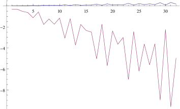
Figure 1: $\Gamma^{\scriptscriptstyle(1)}_{\mathrm{cyc}^{n}}$ plotted in units of $\log R$, from $n=1$ to 32. The blue line is for $\ell=1$ while the purple line is for $\ell=2$.

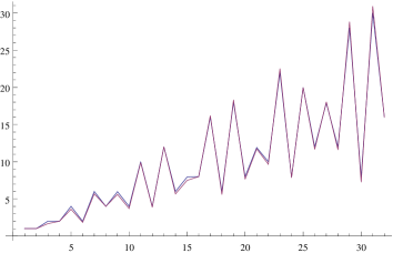
Figure 2: $\Gamma^{\scriptscriptstyle(1)}_{\mathrm{cyc}^{n}}$ plotted in units of $\Gamma^{\scriptscriptstyle(1)}_{\mathrm{Rac}_{\ell}}$, from $n=1$ to 32. The blue line is for $\ell=1$ while the purple line is for $\ell=2$.

In order to better illustrates the behavior of the one-loop free energy of $\mathrm{cyc}^{n}$ with respect to $n$ and $\ell$, we also display in Figure 2 a plot of $\Gamma^{\scriptscriptstyle(1)}_{\mathrm{cyc}^{n}}$ for $\ell=1$ and $\ell=2$ for $n=1$ to $32$ (plotted in units of $\ln R$). We see that the two curves are quite well separated, with the magnitudes of $\Gamma^{\scriptscriptstyle(1)}_{\mathrm{cyc}^{n}}$ being much larger for $\ell=2$ than those for $\ell=1$. At first sight this simply reflects the high sensitivity to $\ell$ in these expressions, already visible in (6.22). On the other hand, if we consider the behaviour of ${\Gamma^{\scriptscriptstyle(1)}_{\mathrm{cyc}^{n}}/\Gamma^{\scriptscriptstyle(1)}_{\mathrm{Rac}_{\ell}}}$ for $\ell=1$ and $\ell=2$, displayed in Figure 2, we see that the two graphs almost coincide with each other.

Finally, we turn to the vacuum energy contribution from the full stringy spectrum, i.e. the spectrum encoded in the character obtained from summing (6.12) from $n=2$ to $\infty$. The resulting character is given by [103]

$$\chi^{so(2,4)}_{SU(N);\mathrm{Rac}_{\ell}}(\beta,\,\vec{\alpha})=-\chi^{so(2,4)}_{\mathrm{Rac}_{\ell}}(\beta,\,\vec{\alpha})-\sum_{k=1}^{\infty}{\varphi(k)\over k}\log\left[1-\chi^{so(2,4)}_{\mathrm{Rac}_{\ell}}(k\beta,\,k\vec{\alpha})\right]\,.$$ (6.24)

Applying the formulae (6.3), (6.20) and (6.21) to

$$\chi_{\cal H}^{so(2,4)}(\beta,\vec{\alpha})=\chi_{\log,k}^{so(2,4)}(\beta,\vec{\alpha})=-\log\left[1-\chi^{so(2,4)}_{\mathrm{Rac}_{\ell}}(k\beta,\,k\vec{\alpha})\right]\,,$$ (6.25)

yields

$$\mathsf{f}_{\log,k}^{4,(0)}(\beta)=-\frac{1}{2}\,\sinh^{4}\tfrac{\beta}{2}\,\log\big{[}1-\frac{\sinh(k\ell\beta)}{8\,\sinh^{4}\tfrac{k\beta}{2}}\big{]}\,,$$ (6.26)

$$\begin{split}\mathsf{f}_{\log,k}^{4,(1)}(\beta)=-\frac{1}{3}\,\sinh^{2}\tfrac{\beta}{2}\,\big{(}\sinh^{2}\tfrac{\beta}{2}-3)\,&\log\big{[}1-\frac{\sinh(k\ell\beta)}{8\,\sinh^{4}\tfrac{k\beta}{2}}\big{]}\,\\ &+\frac{k^{2}\,\sinh^{4}\tfrac{\beta}{2}\,\sinh(k\ell\beta)}{\sinh^{2}\tfrac{k\beta}{2}\,\big{(}8\sinh^{4}\tfrac{k\beta}{2}-\sinh(k\ell\beta)\big{)}}\,,\end{split}$$ (6.27)

$$\begin{split}\mathsf{f}_{\log,k}^{4,(2)}(\beta)&=-\log\big{[}1-\frac{\sinh(k\ell\beta)}{8\,\sinh^{4}\tfrac{k\beta}{2}}\big{]}\,+\frac{k^{4}\,\sinh^{4}\tfrac{\beta}{2}\,\sinh^{2}(k\ell\beta)}{2\,\sinh^{4}\tfrac{k\beta}{2}\,\big{(}8\sinh^{4}\tfrac{k\beta}{2}-\sinh(k\ell\beta)\big{)}^{2}}\,\\ &\qquad-\frac{1}{3}k^{2}\big{(}(k^{2}-1)\sinh^{2}\tfrac{\beta}{2}+3\big{)}\frac{\sinh^{2}\tfrac{\beta}{2}\,\sinh(k\ell\beta)}{\sinh^{2}\tfrac{k\beta}{2}\,\big{(}8\sinh^{4}\tfrac{k\beta}{2}-\sinh(k\ell\beta)\big{)}}\,,\end{split}$$ (6.28)

One can check that by expanding the above expression around $\beta=0$ they are devoid of terms of order $\beta^{1}$, $\beta^{3}$ and $\beta^{5}$ respectively. Hence, by virtue of (6.18), $\chi_{\log,k}^{so(2,4)}$ never contributes to the one-loop free energy of the $SU(N)$ matrix model. As a consequence, we eventually find that

$$\Gamma^{(1)}_{SU(N);\mathrm{Rac}_{\ell}}=-\Gamma^{(1)}_{\mathrm{Rac}_{\ell}}\,.$$ (6.29)

Notice finally that some tacit assumptions in this prescription are discussed in [52, 56].

7 Discussion

In this paper we have applied the arbitrary dimensional CIRZ formula obtained in [57] to partially-massless higher-spin gravities. Firstly, we found that all the theories considered in this paper do not have any UV divergence in its one-loop free energy. Concerning the finite part, the non-minimal type-A_ℓ theories in $d+1$ dimensions have

$$\Gamma^{\scriptscriptstyle(1)}_{{\rm A}_{\ell}^{\text{non-min}}}=0\,,$$ (7.1)

which is consistent with the CFT expectation. On the other hand, the minimal type-A_ℓ theories have

$$\Gamma^{\scriptscriptstyle(1)}_{{\rm A}_{\ell}^{\text{min}}}=\left\{\begin{array}[]{cc}\ln R\,a_{\mathrm{Rac}_{\ell}}&\qquad[d=2r]\\ F_{\mathrm{Rac}_{\ell}}&\qquad[d=2r+1]\end{array}\right..$$ (7.2)

Concerning the type-B_ℓ theories, we find an analogous result for even $d$

$$\Gamma^{\scriptscriptstyle(1)}_{{\rm B}_{\ell}^{\text{non-min}}}=0\,,\qquad\Gamma^{\scriptscriptstyle(1)}_{{\rm B}_{\ell}^{\text{min}}}=\tfrac{1}{2}\,\ln R\,a_{\mathrm{Di}_{\ell}}\,,$$ (7.3)

but for odd $d$, we do not find a relation between the AdS one-loop free energy and the free energy of the order-$\ell$ free fermion. These results have been obtained previously in the $\ell=1$ case [42, 43] and for the type-A₂ case for $d$ up to 20 [46]. The results about the minimal theories may fit in with the holographic conjecture by introducing a shift in the dictionary between the bulk coupling constant $g$ and the number of conformal fields $N$ [42, 43]: $g^{-1}=N-1\,.$ Meanwhile, the results for the putative stringy dualities seem to suggest the relation $g^{-1}=N^{2}$ [52]. We suggest the same interpretation for our results, which have been derived for arbitrary $d$ and $\ell$.

In obtaining our results for partially-massless higher-spin theories using CIRZ, we could reconfirm that the zeta function regularization renders finite not only the divergences from UV but also those from the sum over spectrum. However, as we are considering non-unitary theories, several signs of non-unitarity show up in the form of IR divergences. They arise in the $\beta$ integral for the large $\beta$ region. The parameter $\beta$ has a clear meaning of the inverse energy scale, as one can see from its role in the character: small $\beta$ corresponds to high energy and large $\beta$ to small energy. The lowest energy of the theory decreases as $\ell$ increases, and we could see that the $\beta$ integral starts to diverge for $\ell\geq\frac{d}{4}$ and $\ell\geq\frac{d+2}{4}$ in the type-A_ℓ and type-B_ℓ theories, respectively. From the AdS perspective, the divergences arising for higher $\ell$ are caused by the fields with vanishing $\bar{\Delta}=\Delta-\frac{d}{2}$, which can be interpreted as the AdS counterpart of the IR divergence of the massless fields in flat spacetime. This kind of IR divergence could be removed by an analytic continuation in $\ell$. As $\ell$ increases further, the theory contains fields with negative $\Delta$ (hence negative energy states) for $\ell\geq\frac{d}{2}$ and $\ell\geq\frac{d+1}{2}$ in type-A_ℓ and type-B_ℓ theories, respectively. Interestingly, these bounds correspond to that for the IR divergence of the CFT, meaning the divergence of the CFT zeta function in the large $\beta$ region. Above this bound, the even $d$ free energy develops an imaginary part, which could be exactly calculated. It would be interesting to better understand the physical implications of these issues for both AdS and CFT sides.

Appendix A Type-B_ℓ minimal model

In this appendix, we spell out the decomposition of the antisymmetrized tensor product of two $\mathrm{Di}_{\ell}$ singletons in arbitrary dimensions, which corresponds to the spectrum of the minimal type-B_ℓ theory. To do so, we will use the previously introduced characters expressed in terms of the variables

$$q:=e^{-\beta}\,,\qquad\text{and}\qquad x_{k}:=e^{i\alpha_{k}}\,,\quad k=1,\dots,r\,,$$ (A.1)

instead of $\beta$ and $\vec{\alpha}$. For instance, the character of the $\mathrm{Di}_{\ell}$ singleton then reads

$$\chi^{so(2,d)}_{\mathrm{Di}_{\ell}}(q,\bar{x})=q^{\frac{d+1-2\ell}{2}}\,(1-q^{2\ell-1})\,\chi^{so(d)}_{\boldsymbol{\frac{1}{2}}}(\bar{x})\,\mathcal{P}_{d}(q,\bar{x})\,,$$ (A.2)

with $\bar{x}=(x_{1},\dots,x_{r})$ and

$$\mathcal{P}_{d}(q,\bar{x})=\frac{1}{(1-q)^{d-2r}}\,\prod_{k=1}^{r}\,\frac{1}{(1-qx_{k})(1-qx_{k}^{-1})}\,.$$ (A.3)

Characters of the $so(d)$ algebra can be found in [57] or the textbooks [104, 105]. For more details on character of the conformal algebra, see e.g. [106, 107, 108].

A.1 Odd $d$

In order to decompose the plethysm of two $\mathrm{Di}_{\ell}$ singletons using characters, we need to decompose

$$\frac{1}{2}\,\big{(}\chi^{so(2,d)}_{\mathrm{Di}_{\ell}}(q,\bar{x})\big{)}^{2}\pm\frac{1}{2}\,\chi^{so(2,d)}_{\mathrm{Di}_{\ell}}(q^{2},\bar{x}^{2})$$ (A.4)

into a sum of characters of irreducible $so(2,d)$ modules. Knowing the decomposition of the tensor product of two $\mathrm{Di}_{\ell}$ singletons, i.e. the first term in the above equation, we can simply focus on the second term. To deal with it, we will need a few key identities, namely:

• The $\mathcal{P}_{d}$ function evaluated in $(q^{2},x_{1}^{2},\dots,x_{r}^{2})$ can be factorized into a product of two such functions

  $$\mathcal{P}_{d}(q^{2},\bar{x}^{2})=\mathcal{P}_{d}(q,\bar{x})\,\mathcal{P}_{d}(-q,\bar{x})\,,$$ (A.5)

  which can in turn be expanded as the series

  $$\mathcal{P}_{d}(\pm q,\bar{x})=\frac{1}{1-q^{2}}\,\sum_{s=0}^{\infty}(\pm q)^{s}\,\chi_{(s)}^{so(d)}(\bar{x})\,.$$ (A.6)

• The character of the spin-$\tfrac{1}{2}$ $so(d)$ representation can be expanded as

  $$\chi^{so(d)}_{\boldsymbol{\frac{1}{2}}}(\bar{x}^{2})=\sum_{m=0}^{r}\epsilon_{m}\chi^{so(d)}_{(1^{r-m})}(\bar{x})\,,\qquad\epsilon_{m}:=(-1)^{m(m+1)/2}\,.$$ (A.7)

• Finally, the product of two $so(d)$ characters can be decomposed according to the tensor product rule.

Using the above properties, one ends up with the decomposition

$$\chi_{\mathrm{Di}_{\ell}}^{so(2,d)}(q^{2},\bar{x}^{2}) = \epsilon_{r}\sum_{t=-\ell+1}^{\ell-1}\chi^{so(2,d)}_{[d-2t-1;0]}(q,\bar{x})+\epsilon_{r-1}\sum_{t=1,3,\dots}^{2\ell-3}\Big{[}\chi^{so(2,d)}_{[d+t-1;0]}(q,\bar{x})-\chi^{so(2,d)}_{[d-t-1;0]}(q,\bar{x})\Big{]}$$ (A.8)

$$\qquad\quad-\sum_{m=0}^{r-1}\epsilon_{m}\sum_{t=1,3,\dots}^{2\ell-1}\sum_{s=1}^{\infty}(-1)^{s}\chi^{so(2,d)}_{[s+d-t-1;s,1^{r-1-m}]}(q,\bar{x})$$

$$\qquad\qquad-\sum_{m=0}^{r-1}\epsilon_{m}\sum_{t=1,3,\dots}^{2\ell-3}\sum_{s=1}^{\infty}(-1)^{s}\chi^{so(2,d)}_{[s+d-t-1;s,1^{r-1-m}]}(q,\bar{x})\,.$$

Due to the presence of the alternating signs $\epsilon_{m}$ in the above expression, the spectrum of the minimanl type-B_ℓ model depends on the parity of the integer part of the rank $r$. Introducing

$$\bigoplus_{t\,\,{\rm odd}}:=\bigoplus_{t=1,3,\dots}^{2\ell-1}\oplus\bigoplus_{t=1,3,\dots}^{2\ell-3}\,,$$ (A.9)

the four possible cases read as follow:

• Even rank $r=2n$ with $n=2p$:

  $$\mathrm{Di}_{\ell}^{\wedge 2} \cong \bigoplus_{t=1,3,\dots}^{2\ell-3}\mathcal{D}\big{(}d-t-1;0\big{)}\,\,\oplus\,\,\bigoplus_{t=2}^{2\ell-2}\,\,\bigoplus_{m=0}^{r-1}\,\,\bigoplus_{s=1}^{\infty}\mathcal{D}\big{(}s+d-t-1;s,1^{m}\big{)}$$

  $$\qquad\oplus\bigoplus_{t\,\,{\rm odd}}\,\,\bigoplus_{m=0,3\,\,{\rm mod}4}\,\,\bigoplus_{s=2,4,\dots}^{\infty}\mathcal{D}\big{(}s+d-t-1;s,1^{m}\big{)}$$

  $$\qquad\oplus\bigoplus_{t\,\,{\rm odd}}\,\,\bigoplus_{m=1,2\,\,{\rm mod}4}\,\,\bigoplus_{s=1,3,\dots}^{\infty}\mathcal{D}\big{(}s+d-t-1;s,1^{m}\big{)}\,;$$

• Even rank $r=2n$ with $n=2p+1$:

  $$\mathrm{Di}_{\ell}^{\wedge 2} \cong \bigoplus_{t=-\ell+1}^{\ell-1}\mathcal{D}\big{(}d-2t-1;0\big{)}\oplus\bigoplus_{t=1,3,\dots}^{2\ell-3}\mathcal{D}\big{(}d+t-1;0\big{)}$$ (A.11)

  $$\qquad\oplus\bigoplus_{t\,\,{\rm odd}}\,\,\bigoplus_{m=1,2\,\,{\rm mod}\,4}\,\,\bigoplus_{s=2,4,\dots}^{\infty}\mathcal{D}\big{(}s+d-t-1;s,1^{m}\big{)}$$

  $$\qquad\quad\oplus\bigoplus_{t\,\,{\rm odd}}\,\,\bigoplus_{m=0,3\,\,{\rm mod}\,4}\,\,\bigoplus_{s=1,3,\dots}^{\infty}\mathcal{D}\big{(}s+d-t-1;s,1^{m}\big{)}$$

  $$\qquad\qquad\quad\oplus\bigoplus_{t=2}^{2\ell-2}\,\,\bigoplus_{m=0}^{r-1}\,\,\bigoplus_{s=1}^{\infty}\mathcal{D}\big{(}s+d-t-1;s,1^{m}\big{)}\,;$$

• Even rank $r=2n+1$ with $n=2p$:

  $$\mathrm{Di}_{\ell}^{\wedge 2} \cong \bigoplus_{t=-\ell+1}^{\ell-1}\mathcal{D}\big{(}d-2t-1;0\big{)}\oplus\bigoplus_{t=1,3,\dots}^{2\ell-3}\mathcal{D}\big{(}d-t-1;0\big{)}$$ (A.12)

  $$\qquad\oplus\bigoplus_{t\,\,{\rm odd}}\,\,\bigoplus_{m=0,1\,\,{\rm mod}\,4}\,\,\bigoplus_{s=2,4,\dots}^{\infty}\mathcal{D}\big{(}s+d-t-1;s,1^{m}\big{)}$$

  $$\qquad\quad\oplus\bigoplus_{t\,\,{\rm odd}}\,\,\bigoplus_{m=2,3\,\,{\rm mod}\,4}\,\,\bigoplus_{s=1,3,\dots}^{\infty}\mathcal{D}\big{(}s+d-t-1;s,1^{m}\big{)}$$

  $$\qquad\qquad\quad\oplus\bigoplus_{t=2}^{2\ell-2}\,\,\bigoplus_{m=0}^{r-1}\,\,\bigoplus_{s=1}^{\infty}\mathcal{D}\big{(}s+d-t-1;s,1^{m}\big{)}\,;$$

• Even rank $r=2n+1$ with $n=2p+1$:

  $$\mathrm{Di}_{\ell}^{\wedge 2} \cong \bigoplus_{t=1,3,\dots}^{2\ell-3}\mathcal{D}\big{(}d+t-1;0\big{)}\oplus\bigoplus_{t=2}^{2\ell-2}\,\,\bigoplus_{m=0}^{r-1}\,\,\bigoplus_{s=1}^{\infty}\mathcal{D}\big{(}s+d-t-1;s,1^{m}\big{)}$$

  $$\qquad\oplus\bigoplus_{t\,\,{\rm odd}}\,\,\bigoplus_{m=0,1\,\,{\rm mod}4}\,\,\bigoplus_{s=1,3,\dots}^{\infty}\mathcal{D}\big{(}s+d-t-1;s,1^{m}\big{)}$$

  $$\qquad\oplus\bigoplus_{t\,\,{\rm odd}}\,\,\bigoplus_{m=2,3\,\,{\rm mod}4}\,\,\bigoplus_{s=2,4,\dots}^{\infty}\mathcal{D}\big{(}s+d-t-1;s,1^{m}\big{)}\,.$$

A.2 Even $d$

As recalled previously, in odd-dimensional AdS space (i.e. when $d=2r$) one can consider a chiral $\mathrm{Di}_{\ell}$ singleton, that is, a Weyl spinor subject to a higher-order Dirac equation on the $d$-dimensional conformal boundary. As a consequence, a first truncation, before the minimal model, of the type-B_ℓ theory is the chiral type-B_ℓ,± whose spectrum is given by the tensor product of two $\mathrm{Di}_{\ell}$ singleton of same chirality. This decomposition is presented hereafter.

A.2.1 Chiral Flato-Fronsdal

The main ingredient in obtaining the decomposition displayed below is the $so(2)\oplus so(d)$ decomposition of a chiral singleton module, namely

$$\chi^{so(d)}_{\mathrm{Di}_{\ell,\pm}}(q,\bar{x})=\sum_{s=0}^{\infty}q^{\frac{d+1-2\ell}{2}+s}\,\Big{(}\sum_{k=0}^{\ell-1}q^{2k}\,\chi_{(s+\frac{1}{2},\frac{1}{2}_{\pm})}^{so(d)}(\bar{x})\,+\sum_{k=0}^{\ell-2}q^{2k+1}\,\chi^{so(d)}_{(s+\frac{1}{2},\frac{1}{2}_{\mp})}(\bar{x})\Big{)}\,,$$ (A.14)

where the second term appears only for $\ell>1$. With this identity at hand, one can show that

• Rank $r=2n$: The tensor product of two $\mathrm{Di}_{\ell}$ singleton of the same chirality decomposes as follows:

  $$\mathrm{Di}_{\ell,\pm}^{\otimes 2} = \bigoplus_{t=-2\ell+2,-2\ell+4,\dots}^{2\ell-2}\mathcal{D}\big{(}d-t-1;0\big{)}\oplus\bigoplus_{m=1}^{n}\bigoplus_{t=1,3,\dots}^{2\ell-1}\bigoplus_{s=1}^{\infty}\mathcal{D}\big{(}s+d-t-1;s,1_{\pm}^{2m-1}\big{)}$$ (A.15)

  $$\qquad\oplus\bigoplus_{m=1}^{n}\bigoplus_{t=1,3,\dots}^{2\ell-3}\bigoplus_{s=1}^{\infty}\mathcal{D}\big{(}s+d-t-1;s,1_{\mp}^{2m-1}\big{)}$$

  $$\qquad\qquad\qquad\oplus 2\,\bigoplus_{m=0}^{n-1}\bigoplus_{t=2,4,\dots}^{2\ell-2}\bigoplus_{s=1}^{\infty}\mathcal{D}\big{(}s+d-t-1;s,1^{2m}\big{)}\,.$$

  Notice in particular that there is no graviton in this spectrum, but the massive scalars are present. The tensor product of two opposite chiralities $\mathrm{Di}_{\ell}$ singleton reads

  $$\mathrm{Di}_{\ell,+}\otimes\mathrm{Di}_{\ell,-} = \bigoplus_{t=-2\ell+3,-2\ell+5,\dots}^{2\ell-3}\mathcal{D}\big{(}d-t-1;0\big{)}\oplus\bigoplus_{m=1}^{n}\bigoplus_{s=1}^{\infty}\bigoplus_{t=2,4,\dots}^{2\ell-2}\mathcal{D}\big{(}s+d-t-1;s,1_{\pm}^{2m-1}\big{)}$$ (A.16)

  $$\qquad\oplus\bigoplus_{m=1}^{n}\bigoplus_{s=1}^{\infty}\bigoplus_{t=2,4,\dots}^{2\ell-2}\mathcal{D}\big{(}s+d-t-1;s,1_{\mp}^{2m-1}\big{)}$$

  $$\qquad\qquad\oplus\bigoplus_{m=0}^{n-1}\bigoplus_{s=1}^{\infty}\Big{(}\bigoplus_{t=1,3,\dots}^{2\ell-1}\oplus\bigoplus_{t=1,3,\dots}^{2\ell-3}\Big{)}\mathcal{D}\big{(}s+d-t-1;s,1^{2m}\big{)}\,.$$

• Rank $r=2n+1$: Contrary to the previous case, the tensor product of two $\mathrm{Di}_{\ell}$ singletons of the same chirality which reads

  $$\mathrm{Di}_{\ell,\pm}^{\otimes 2} = \bigoplus_{t=-2\ell+3,-2\ell+5,\dots}^{2\ell-3}\mathcal{D}\big{(}d-t-1;0\big{)}\oplus\bigoplus_{m=0}^{n}\bigoplus_{t=1,3,\dots}^{2\ell-1}\bigoplus_{s=1}^{\infty}\mathcal{D}\big{(}s+d-t-1;s,1^{2m}_{\pm}\big{)}$$ (A.17)

  $$\qquad\quad\oplus\bigoplus_{m=0}^{n}\bigoplus_{t=1,3,\dots}^{2\ell-3}\mathcal{D}\big{(}s+d-t-1;s,1^{2m}_{\mp}\big{)}$$

  $$\qquad\qquad\qquad\oplus 2\bigoplus_{m=1}^{n}\bigoplus_{s=1}^{\infty}\bigoplus_{t=2,4,\dots}^{2\ell-2}\mathcal{D}\big{(}s+d-t-1;s,1^{2m-1}\big{)}\,.$$

  The above does contain a graviton but no longer include the massive scalars. The tensor product of two $\mathrm{Di}_{\ell}$ singletons of opposite chiralities displays the complement of the previous content with respect to the spectrum of the (full) type-B_ℓ theory:

  $$\mathrm{Di}_{\ell,+}\otimes\mathrm{Di}_{\ell,-} = \bigoplus_{t=-2\ell+2,-2\ell+4,\dots}^{2\ell-2}\mathcal{D}\big{(}d-t-1;0\big{)}\oplus\bigoplus_{m=0}^{n}\bigoplus_{s=1}^{\infty}\bigoplus_{t=2,4,\dots}^{2\ell-2}\mathcal{D}\big{(}s+d-t-1;s,1^{2m}_{\pm}\big{)}$$ (A.18)

  $$\qquad\oplus\bigoplus_{m=0}^{n}\bigoplus_{s=1}^{\infty}\bigoplus_{t=2,4,\dots}^{2\ell-2}\mathcal{D}\big{(}s+d-t-1;s,1^{2m}_{\mp}\big{)}$$

  $$\qquad\qquad\oplus\bigoplus_{m=1}^{n}\bigoplus_{s=1}^{\infty}\Big{(}\bigoplus_{t=1,3,\dots}^{2\ell-1}\oplus\bigoplus_{t=1,3,\dots}^{2\ell-3}\Big{)}\mathcal{D}\big{(}s+d-t-1;s,1^{2m-1}\big{)}\,.$$

A.2.2 Minimal model

In order to decompose $\chi^{so(2,d)}_{\mathrm{Di}_{\ell,\pm}}(q^{2},\bar{x}^{2})$ into a sum of characters appearing in (A.15) and (A.17), we need the identity

$$\chi^{so(d)}_{\frac{1}{2}_{\pm}}(\bar{x}^{2})=\sum_{m=0}^{[r/2]}(-1)^{m}\,\chi^{so(d)}_{(1^{r-2m}_{\pm})}(\bar{x})\,.$$ (A.19)

Using the above property, one can show that for $r=2n$,

$$\chi^{so(2,d)}_{\mathrm{Di}_{\ell,\pm}}(q^{2},\bar{x}^{2}) = (-1)^{n}\sum_{t=-2\ell+2,-2\ell+4,\dots}^{2\ell-2}\chi^{so(2,d)}_{[d-t-1;0]}(q,\bar{x})$$ (A.20)

$$\qquad+\sum_{m=1}^{n}(-1)^{n+m+1}\sum_{s=1}^{\infty}(-1)^{s}\Big{[}\sum_{t=1,3,\dots}^{2\ell-1}\chi^{so(2,d)}_{[s+d-t-1;s,1^{2m-1}_{\pm}]}(q,\bar{x})$$

$$\qquad\qquad\quad+\sum_{t=1,3,\dots}^{2\ell-3}\chi^{so(2,d)}_{[s+d-t-1;s,1^{2m-1}_{\mp}]}(q,\bar{x})\Big{]}\,,$$

whereas for $r=2n+1$,

$$\chi^{so(2,d)}_{\mathrm{Di}_{\ell,\pm}}(q^{2},\bar{x}^{2}) = (-1)^{n}\sum_{t=1,3,\dots}^{2\ell-3}\Big{[}\chi^{so(2,d)}_{[d+t-1;0]}(q,\bar{x})-\chi^{so(2,d)}_{[d-t-1;0]}(q,\bar{x})\Big{]}$$ (A.21)

$$\qquad+\sum_{m=0}^{n}(-1)^{n+m+1}\sum_{s=1}^{\infty}(-1)^{s}\Big{[}\sum_{t=1,3,\dots}^{2\ell-1}\chi^{so(2,d)}_{[s+d-t-1;s,1^{2m}_{\pm}]}(q,\bar{x})$$

$$\qquad\qquad\quad+\sum_{t=1,3,\dots}^{2\ell-3}\chi^{so(2,d)}_{[s+d-t-1;s,1^{2m}_{\mp}]}(q,\bar{x})\Big{]}\,,$$

and hence

• Even rank $r=2n$ with $n=2p$:

  $$\mathrm{Di}_{\ell,\pm}^{\wedge 2} \cong \bigoplus_{m=3\,\,{\rm mod}\,\,4}\,\,\bigoplus_{s=2,4,\dots}^{\infty}\bigoplus_{t=1,3,\dots}^{2\ell-1}\mathcal{D}\big{(}s+d-t-1;s,1_{\pm}^{m}\big{)}$$

  $$\qquad\oplus\bigoplus_{m=3\,\,{\rm mod}\,\,4}\,\,\bigoplus_{s=2,4,\dots}^{\infty}\bigoplus_{t=1,3,\dots}^{2\ell-3}\mathcal{D}\big{(}s+d-t-1;s,1_{\mp}^{m}\big{)}$$

  $$\qquad\qquad\oplus\bigoplus_{m=1\,\,{\rm mod}\,\,4}\,\,\bigoplus_{t=1,3,\dots}^{2\ell-1}\bigoplus_{s=1,3,\dots}^{\infty}\mathcal{D}\big{(}s+d-t-1;s,1_{\pm}^{m}\big{)}$$

  $$\qquad\qquad\qquad\oplus\bigoplus_{m=1\,\,{\rm mod}\,\,4}\,\,\bigoplus_{s=1,3,\dots}^{\infty}\bigoplus_{t=1,3,\dots}^{2\ell-3}\mathcal{D}\big{(}s+d-t-1;s,1_{\mp}^{m}\big{)}$$

  $$\qquad\qquad\qquad\qquad\oplus\bigoplus_{m=0}^{n-1}\,\,\bigoplus_{s=1}^{\infty}\bigoplus_{t=2,4,\dots}^{2\ell-2}\mathcal{D}\big{(}s+d-t-1;s,1^{2m}\big{)}\,;$$

• Even rank $r=2n$ with $n=2p+1$:

  $$\mathrm{Di}_{\ell,\pm}^{\wedge 2} \cong \bigoplus_{t=-2\ell+2,-2\ell+4,\dots}^{2\ell-2}\mathcal{D}\big{(}d-t-1;0\big{)}$$

  $$\qquad\oplus\bigoplus_{m=1\,\,{\rm mod}\,\,4}\,\,\bigoplus_{s=2,4,\dots}^{\infty}\bigoplus_{t=1,3,\dots}^{2\ell-1}\mathcal{D}\big{(}s+d-t-1;s,1_{\pm}^{m}\big{)}$$

  $$\qquad\qquad\oplus\bigoplus_{m=1\,\,{\rm mod}\,\,4}\,\,\bigoplus_{s=2,4,\dots}^{\infty}\bigoplus_{t=1,3,\dots}^{2\ell-3}\mathcal{D}\big{(}s+d-t-1;s,1_{\mp}^{m}\big{)}$$

  $$\qquad\qquad\qquad\oplus\bigoplus_{m=3\,\,{\rm mod}\,\,4}\,\,\bigoplus_{s=1,3,\dots}^{\infty}\bigoplus_{t=1,3,\dots}^{2\ell-1}\mathcal{D}\big{(}s+d-t-1;s,1_{\pm}^{m}\big{)}$$

  $$\qquad\qquad\qquad\qquad\oplus\bigoplus_{m=3\,\,{\rm mod}\,\,4}\,\,\bigoplus_{s=1,3,\dots}^{\infty}\bigoplus_{t=1,3,\dots}^{2\ell-3}\mathcal{D}\big{(}s+d-t-1;s,1_{\mp}^{m}\big{)}$$

  $$\qquad\qquad\qquad\qquad\qquad\oplus\bigoplus_{m=0}^{n-1}\,\,\bigoplus_{t=2,4,\dots}^{2\ell-2}\bigoplus_{s=1}^{\infty}\mathcal{D}\big{(}s+d-t-1;s,1^{2m}\big{)}\,;$$

• Even rank $r=2n+1$ with $n=2p$:

  $$\mathrm{Di}_{\ell,\pm}^{\wedge 2} \cong \bigoplus_{t=1,3,\dots}^{2\ell-3}\mathcal{D}\big{(}d-t-1;0\big{)}$$

  $$\qquad\oplus\bigoplus_{m=0\,\,{\rm mod}\,\,4}\bigoplus_{s=2,4,\dots}^{\infty}\bigoplus_{t=1,3,\dots}^{2\ell-1}\mathcal{D}\big{(}s+d-t-1;s,1^{m}_{\pm}\big{)}$$

  $$\qquad\qquad\oplus\bigoplus_{m=0\,\,{\rm mod}\,\,4}\bigoplus_{s=2,4,\dots}^{\infty}\bigoplus_{t=1,3,\dots}^{2\ell-3}\mathcal{D}\big{(}s+d-t-1;s,1^{m}_{\mp}\big{)}$$

  $$\qquad\qquad\qquad\oplus\bigoplus_{m=2\,\,{\rm mod}\,\,4}\bigoplus_{s=1,3,\dots}^{\infty}\bigoplus_{t=1,3,\dots}^{2\ell-1}\mathcal{D}\big{(}s+d-t-1;s,1^{m}_{\pm}\big{)}$$

  $$\qquad\qquad\qquad\qquad\oplus\bigoplus_{m=0\,\,{\rm mod}\,\,4}\bigoplus_{s=1,3,\dots}^{\infty}\bigoplus_{t=1,3,\dots}^{2\ell-3}\mathcal{D}\big{(}s+d-t-1;s,1^{m}_{\mp}\big{)}$$

  $$\qquad\qquad\qquad\qquad\quad\oplus\bigoplus_{m=1}^{n}\bigoplus_{s=1}^{\infty}\bigoplus_{t=2,4,\dots}^{2\ell-2}\mathcal{D}\big{(}s+d-t-1;s,1^{2m-1}\big{)}\,;$$

• Even rank $r=2n+1$ with $n=2p+1$:

  $$\mathrm{Di}_{\ell,\pm}^{\wedge 2} \cong \bigoplus_{t=1,3,\dots}^{2\ell-3}\mathcal{D}\big{(}d+t-1;0\big{)}$$

  $$\qquad\oplus\bigoplus_{m=0\,\,{\rm mod}\,\,4}\,\,\bigoplus_{s=1,3,\dots}^{\infty}\bigoplus_{t=1,3,\dots}^{2\ell-1}\mathcal{D}\big{(}s+d-t-1;s,1^{2m}_{\pm}\big{)}$$

  $$\qquad\qquad\oplus\bigoplus_{m=0\,\,{\rm mod}\,\,4}\,\,\bigoplus_{s=1,3,\dots}^{\infty}\bigoplus_{t=1,3,\dots}^{2\ell-3}\mathcal{D}\big{(}s+d-t-1;s,1^{2m}_{\mp}\big{)}$$

  $$\qquad\qquad\qquad\oplus\bigoplus_{m=2\,\,{\rm mod}\,\,4}\,\,\bigoplus_{s=2,4,\dots}^{\infty}\bigoplus_{t=1,3,\dots}^{2\ell-1}\mathcal{D}\big{(}s+d-t-1;s,1^{2m}_{\pm}\big{)}$$

  $$\qquad\qquad\qquad\qquad\oplus\bigoplus_{m=2\,\,{\rm mod}\,\,4}\,\,\bigoplus_{s=2,4,\dots}^{\infty}\bigoplus_{t=1,3,\dots}^{2\ell-3}\mathcal{D}\big{(}s+d-t-1;s,1^{2m}_{\mp}\big{)}$$

  $$\qquad\qquad\qquad\qquad\qquad\oplus\bigoplus_{m=1}^{n}\bigoplus_{s=1}^{\infty}\bigoplus_{t=2,4,\dots}^{2\ell-2}\mathcal{D}\big{(}s+d-t-1;s,1^{2m-1}\big{)}\,.$$