Model-based resonance tracking of linear systems

Abstract

The present paper develops recursive algorithms to track shifts in the resonance frequency of linear systems in real time. To date, automatic resonance tracking has been limited to non-model-based approaches, which rely solely on the phase difference between a specific input and output of the system. Instead, we propose a transformation of the system into a complex-valued representation, which allows us to abstract the resonance shifts as an exogenous disturbance acting on the excitation frequency, perturbing the excitation frequency from the natural frequency of the plant. We then discuss the resonance tracking task in two parts: recursively identifying the frequency disturbance and incorporating an update of the excitation frequency in the algorithm. The complex representation of the system simplifies the design of resonance tracking algorithms due to the applicability of well-established techniques. We discuss the stability of the proposed scheme, even in cases that seriously challenge current phase-based approaches, such as nonmonotonic phase differences and multiple-input multiple-output systems. Numerical simulations further demonstrate the performance of the proposed resonance tracking scheme.

Keywords adaptive control  $\cdot$ complex variables  $\cdot$ frequency tracking  $\cdot$ resonance.

1 Introduction

Precisely tracking the resonance frequency of oscillating systems is of great interest in resonant sensing [Hauptmann1991, Boisen2011] and in the driving of vibrating loads [Claeyssen2003, Gokcek2005]. Resonant sensors, the function of which relies on the resonant characteristic of a vibrating structure, have been proposed for a wide range of measurements and instruments, including thermometers [Larsen2011], accelerometers [Aikele2001], viscometers [Brack2016], humidity sensors [Sheng2011], water cut measurements [Avila2017] and gyroscopes [Raman2009, Fei2015]. In terms of miniaturization and increased sensitivity, microelectromechanical systems (MEMS) with vibrating cantilevers have emerged as an appealing solution, and achievements such as atomic force microscopy in space [Bentley2016] and mass detection in the range of atto- and zeptograms [Boisen2011] have been reported. Furthermore, resonant electromechanical actuators have been widely proposed for power electronics [Li2016, Singh2014, Bosshard2014, Choi2006], ultrasonic applications [Liu2015], thermosonic wire bonding [Zhang2015] and acoustic particle trapping [Hammarstroem2014].

To increase the sensitivity of sensors and the power output of vibrating actuators, designers adopt systems with “sharp” resonances (low damping and a high quality factor) [Hammarstroem2014]. As a drawback, this design leads to diminished performance when the excitation frequency deviates even slightly from the resonance frequency due to the inherently narrow bandwidth of the system. Even for actuators that have been designed to operate at a constant resonance, shifts from the designed operating frequency may occur because of environmental changes such as temperature and humidity variations [Ferguson2005], aging of the device [Sun2002] or changes in the load [Zhang2015, Bosshard2014]. As a remedy, designers resort to feedback resonance tracking control to compensate for these shifts and achieve maximum efficiency [Gokcek2005, Li2016]. In the case of sensing applications based on changes in the resonance frequency with the measured quantity, the use of feedback control is unavoidable, and the performance of the control system directly affects the sensitivity, resolution and bandwidth of the sensor [Sun2002, Albrecht1991].

Regardless of the application, the phase locked loop (PLL) is the typical scheme for resonance tracking [Sun2002, Brack2016]. The self-sustained oscillation (SSO) scheme [Lulec2016, Gorreta2016] has also been proposed to induce excitation at resonance frequencies. Both techniques achieve tracking of the resonance frequency by maintaining a constant phase difference between the input and the output of the system. Their main difference lies in the fact that the PLL utilizes an external oscillator to generate the signal that excites the system. In contrast, for the SSO case, the excitation signal is generated by the oscillating structure itself; the system output is amplified and phase-shifted before it is fed back to the system. The design and analysis of the PLL and SSO resonant tracking schemes connected with a single-input single-output (SISO) 2^nd-order system have been extensively discussed by many authors for various applications [Sun2002, Park2009, Aikele2001, SohanianHaghighi2012, Lulec2016, Brack2016]. A drawback of these resonance tracking approaches is that they are far from being model-based; more importantly, however, the closed-loop robustness and stability cannot be guaranteed. This situation is true even for linear SISO systems if the phase difference between the input and output signal is nonmonotonic. This problem has been pointed out for piezoelectric actuators and multi-degree-of-freedom systems, where resonance and anti-resonance frequencies are present [Hayashi1992, Zhang2015, Brack2016a, Liu2015].

To supplement the two techniques mentioned above, specialized resonance tracking algorithms have been developed for specific cases. In the absence of phase information, an algorithm that detects the maximum of the output signal has been employed in piezoresponse force microscopy [Rodriguez2007]. A maximum power tracking adaptive approach for the driving of resonant loads was proposed in [Gokcek2005]; in this approach, a small sinusoidal perturbation signal is added to the driving signal to estimate the derivative of the absorbed power and update the excitation frequency. A control algorithm that tunes the system to a specific resonance frequency was developed to address the issue of online modal frequency matching in vibratory gyroscopes [Park2009]. Other specialized schemes employ controller scheduling [Song2016] and fuzzy logic [Zhang2015]. Nonetheless, all of the previous approaches were developed for operation with a specific system, which makes it difficult to generalize the approach and may require multiple driving signals. Moreover, the application of these schemes has been limited to SISO systems, making their extension to multiple-input multiple-output (MIMO) systems rather complicated.

The PLL and SSO techniques have both proven their capabilities in numerous applications. By neglecting the system model, these techniques are sufficiently general and therefore applicable in many cases. On the other hand, tuning the controller parameters may be tedious, and theoretical analysis of the closed-loop performance still requires a mathematical description of the system. Nevertheless, if a description of the system is available, a model-based controller design approach is expected to yield improved performance. Here, we consider control algorithms that are able to track the resonance of linear models. We introduce a representation of the oscillating plant, which splits the system into a linear time-invariant (LTI) model and an abstract shift of the frequency exciting the system. This model representation simplifies the application of well-established control and estimation techniques.

The remainder of this paper is organized as follows. The resonance tracking problem is formalized in Section 2. The complex representation of oscillating linear systems and the abstract modeling of resonance shifts are introduced in Section 3. Section LABEL:sec:freqtracking presents the estimation of the resonance shift and the update of the excitation frequency. Implementation considerations and numerical simulations are discussed in Section LABEL:sec:simulations. Section LABEL:sec:conclusion concludes the paper.

2 Problem statement

We consider the following discrete-time linear model: rCl x_k+1 & = ~A x_k + ~B u_k + ~w_k
y_k = ~C x_k + ~D u_k + ~v_k where $x_{k}\in\mathbb{R}^{n}$, $u_{k}\in\mathbb{R}^{m}$, and $y_{k}\in\mathbb{R}^{p}$ denote the state, input and output vectors, respectively, at the discrete sampling instances $k\in\mathbb{N}$ and $\tilde{w}_{k}\sim\mathcal{N}(0,Q)$ and $\tilde{v}_{k}\sim\mathcal{N}(0,R)$ are uncorrelated additive white Gaussian noise used to model the disturbance input and the measurement noise, respectively. The system matrices depend on an unknown parameter vector, $\kappa$, such as $\tilde{A}(\kappa)$, $\tilde{B}(\kappa)$, $\tilde{C}(\kappa)$ and $\tilde{D}(\kappa)$. The vector $\kappa$ may be time-varying: in such cases, the system (2-2) becomes linear time-varying (LTV), which we indicate by explicitly adding the subscript $k$ to the system matrices, e.g., $\tilde{A}_{k}$.

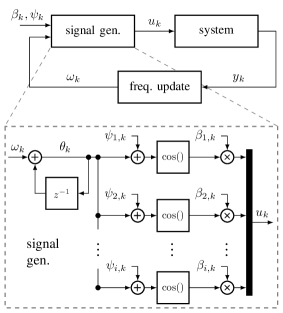
Figure 1: Schematic of the frequency tracking problem.

We assume that the system has at least one pair of conjugated complex eigenvalues corresponding to the resonance frequency of interest. We denote the eigenvalue of interest by $\tilde{\lambda}_{s}$ and its corresponding resonance by $\tilde{\omega}_{\lambda}=\arg\tilde{\lambda}_{s}>0$. The system is subjected to a sinusoidal input $u_{i,k}=\beta_{i,k}\cos(\theta_{k}+\psi_{i,k})$, where $\beta_{i,k}\in\mathbb{R}_{\geq 0}$ and $\psi_{i,k}\in(-\pi,\,\pi]$ denote the instantaneous amplitude and phase, respectively, of $u_{i,k}$, the $i$^th component of $u_{k}$. The common reference phase is denoted by $\theta_{k}\in\mathbb{R}$ and evolves according to

$$\theta_{k+1}=\theta_{k}+\omega_{k}$$ (1)

where $\omega_{k}$ is the normalized angular frequency of the excitation.

The goal of this study is to develop a recursive scheme that detects the resonance frequency of the linear system (2-2). More precisely, we aim to develop a recursive algorithm that drives the excitation frequency $\omega_{k}$ towards $\tilde{\omega}_{\lambda}$. A schematic representation of the structure of the resonance tracking problem and the composition of $u_{k}$ is shown in Fig. 1.

3 Complex state-space model

In this section, we introduce a transformation of the oscillating system into an equivalent description where the state, input and output variables are represented as complex envelopes of sinusoidal signals.

3.1 CSS representation

We discuss the transformation for a general LTV system: rCl x_k+1 & = ~A_k x_k + ~B_k u_k + ~w_k
y_k = ~C_k x_k + ~D_k u_k + ~v_k excited by the sinusoidal input $u_{k}$. Inspired by [Mcloskey1999, Sun2002], we write the state and output variables in an amplitude-phase formulation, $x_{i,k}=\alpha_{i,k}\cos(\theta_{k}+\phi_{i,k})$ and $y_{i,k}=\delta_{i,k}\cos(\theta_{k}+\varphi_{i,k})$, where $\alpha_{i,k}$, $\delta_{i,k}$, $\phi_{i,k}$ and $\varphi_{i,k}$ are components of time-varying vectors of appropriate dimensions. Substituting the phase-amplitude expressions into (3.1), the time update for the $i$^th component of $x_{k}$ is

$$\alpha_{i,k+1}\cos(\theta_{k}+\omega_{k}+\phi_{i,k+1})=\sum_{l=1}^{n}\tilde{A}_{il,k}\alpha_{l,k}\cos(\theta_{k}+\phi_{l,k})\IEEEnonumber+\sum_{l=1}^{m}\tilde{B}_{il,k}\beta_{l,k}\cos(\theta_{k}+\psi_{l,k})$$ (2)

where $\tilde{A}_{il,k}$ and $\tilde{B}_{il,k}$ are the components of the $i$^th row and $l$^th column of the matrices $\tilde{A}_{k}$ and $\tilde{B}_{k}$, respectively. In the previous expressions, we have neglected the effect of $\tilde{w}_{k}$. We use the angle-sum trigonometric identities to expand the terms in (2): rCl 3lα_i,k+1 [ cosθ_k cos(ω_k + ϕ_i,k+1) - sinθ_k sin(ω_k + ϕ_i,k+1) ]
 & = ∑_l=1^n ~A_il,k [ α_i,k ( cosθ_k cosϕ_l,k - sinθ_k sinϕ_l,k ) ] + ∑_l=1^m ~B_il,k [ β_l,k ( cosθ_k cosψ_l,k - sinθ_k sinψ_l,k ) ] which can be compactly written as

$$c_{c,i,k}\cos\theta_{k}+c_{s,i,k}\sin\theta_{k}=\sqrt{c_{c,i,k}^{2}+c_{s,i,k}^{2}}\sin(\theta_{k}+\arctan\frac{c_{c,i,k}}{c_{s,i,k}})=0.$$ (3)

Eq. (3) becomes independent of $\theta_{k}$ by setting $c_{c,i,k}=c_{s,i,k}=0$: rCl α_i,k+1 cos(ω_k + ϕ_i,k+1) & = ∑_l=1^n ~A_il,k α_l,k cosϕ_l,k + ∑_l=1^m ~B_il,k β_l,k cosψ_l,k
α_i,k+1 sin(ω_k + ϕ_i,k+1) = ∑_l=1^n ~A_il,k α_l,k sinϕ_l,k + ∑_l=1^n ~B_il,k β_l,k sinψ_l,k . We introduce the transformation for the $i$^th state component in complex notation, $z_{i,k}=\alpha_{i,k}(\cos\phi_{i,k}+j\sin\phi_{i,k})=\alpha_{i,k}e^{j\phi_{i,k}}$. Similarly, we write the output as $q_{i,k}=\delta_{i,k}e^{j\varphi_{i,k}}$ and the input as $s_{i,k}=\beta_{i,k}e^{j\psi_{i,k}}$. The symbol $j=\sqrt{-1}$ is the imaginary unit. This complex signal form is similar to the complex envelope representation of a bandpass signal in communication channels [Neeser1993] and to the analytic signal [Boashash1992]. Substitution of the complex variables into (3-3) results in the following complex system: rCl z_k+1 & = ( ~A_k z_k + ~B_k s_k + w_k ) e^-j ω_k
q_k = ~C_k z_k + ~D_k s_k + v_k where $w_{k}$ and $v_{k}$ are proper random variables with a complex Gaussian ($\mathcal{CN}$) probability density function, that is, $w_{k}\sim\mathcal{CN}(0,\,Q)$ and $v_{k}\sim\mathcal{CN}(0,\,R)$. The complex envelope of white real-valued Gaussian signals has been shown to be complex proper normal, where the properness arises from the stationarity assumption [Picinbono1994, Neeser1993]. Eq. (3) follows from (3.1) using the same procedure. We refer to the system (3-3) as the complex state space (CSS) representation.

The conversion of an LTV system into the CSS representation can be derived by substituting the analytic signal directly into (3.1-3.1). The derivation is simpler and directly relates each signal to its complex envelope but lacks intuition and reasoning for the complex representation of the variables. The substitution of $u_{k}=s_{k}e^{j\theta_{k}}$ and $\tilde{w}_{k}=w_{k}e^{j\theta_{k}}$ into (3.1) results in

$$x_{k+1}=\tilde{A}_{k}x_{k}+\tilde{B}s_{k}e^{j\theta_{k}}+w_{k}e^{j\theta_{k}}$$ (4)

which is equal to (3) for $x_{k}=z_{k}e^{j\theta_{k}}$ and $x_{k+1}=z_{k+1}e^{j\omega_{k}}e^{j\theta_{k}}$. The evolution of the real part of (4), which is entirely disconnected from the complex part, coincides with (3.1). Furthermore, we apply the same reasoning to derive the continuous-time CSS representation in Appendix LABEL:app:continuousTimeCSS.

3.2 Properties of the CSS representation

Transforming (3.1-3.1) into the CSS representation constitutes an alternative description of the original system. Under equivalent input and noise sequences, the trajectories of $x_{k}$ and $z_{k}$ can be derived from one another. It is therefore expected that the properties of (3.1-3.1) are retained after the transformation. In the following, the relevant properties for the design of the resonance tracking algorithm are discussed.

The state transition matrices of the two systems are closely related. Let $\Phi(k,i)=\prod_{l=i}^{k-1}\tilde{A}_{l}$ be the state transition matrix for the system (3.1-3.1); then, the state transition matrix for the CSS representation (3-3) is

$$\Phi_{c}(k,i)=\prod_{l=i}^{k-1}(\tilde{A}_{l}e^{-j\omega_{l}})=\left(\prod_{l=i}^{k-1}\tilde{A}_{l}\right)e^{-j\sum_{l=i}^{k-1}\omega_{l}}=\Phi(k,i)e^{-j\sum_{l=i}^{k-1}\omega_{l}}$$ (5)

with $\Phi(k,k)=\Phi_{c}(k,k)=I$.

Lemma 1.

Consider the LTV system (3.1-3.1) and the associated CSS representation (3-3). For any given sequence $\omega_{i},\,i=1,2,\dotsc,k$, the system (3-3) is globally exponentially stable if and only if the associated system (3.1-3.1) is globally exponentially stable.

Proof.

The exponential stability of (3.1-3.1) implies that there exist scalars $c_{1}>0$ and $0<\lambda_{\Phi}<1$ such that [Zhou2017, lemma 1]

$$\lVert\Phi(k,i)\rVert\leq c_{1}\lambda_{\Phi}^{k-i},\quad\forall i,k\in\mathbb{N}.$$ (6)

For the CSS representation, $\lVert\Phi_{c}(k,i)\rVert=\lVert\Phi(k,i)\rVert\leq c_{1}\lambda_{\Phi}^{k-i}$, which concludes the global exponential stability of (3-3).

The reverse statement can be shown similarly. ∎

Furthermore, the optimal control and optimal estimation problems for (3-3) and the LTV system are directly connected. Assume an observable system (3.1-3.1), and consider the optimal state observer design problem with an initial state estimate $\hat{x}_{0}=E[x_{0}]$ and variance $P_{x,0}=E[(x_{0}-\hat{x}_{0})^{T}(x_{0}-\hat{x}_{0})]$, where $E[\cdot]$ denotes the expected value. The trajectory of the optimal state estimates and the covariance matrix, $P_{x,k+1|k}$, are given by the Kalman filter equations. Specifically, $P_{x,k+1|k}$ follows the Riccati equation

$$P_{x,k+1|k}=\tilde{A}_{k}P_{x,k|k-1}\tilde{A}_{k}^{T}+Q-\tilde{A}_{k}P_{x,k|k-1}\tilde{C}_{k}^{T}(\tilde{C}_{k}P_{x,k|k-1}\tilde{C}_{k}^{T}+R)^{-1}\tilde{C}_{k}P_{x,k|k-1}\tilde{A}_{k}^{T}.$$ (7)

Lemma 2.

Given the optimal estimation problem for the CSS system (3-3) with the initial conditions $\hat{z}_{0}=E[z_{0}]$ and $P_{z,0}=E[(z_{0}-\hat{z}_{0})^{H}(z_{0}-\hat{z}_{0})]$, (7) then describes the evolution of the optimal covariance, $P_{z,k+1|k}$, for any sequence $\omega_{i},\,i=1,2,\dotsc,k$. Moreover, if $P_{z,0}=P_{x,0}$, then $P_{z,k+1|k}=P_{x,k+1|k},\,\forall k>0$.

Proof.

The system matrices of (3-3) are real-valued, and the noise variables are proper. The optimal estimator for such systems has been shown to be the Kalman filter, which achieves optimality in terms of being unbiased and having minimum variance [Dini2012, remark 6].

We write the Kalman filter equations for the CSS model, presented in a prediction and a correction step, as rCl 3sPrediction step:
^z_k|k-1 & = ( ~A_k ^z_k-1|k-1 + ~B_k s_k ) e^-j ω_k
P