Zeno: Distributed Stochastic Gradient Descent with Suspicion-based Fault-tolerance

Abstract

We present Zeno, a technique to make distributed machine learning, particularly Stochastic Gradient Descent (SGD), tolerant to an arbitrary number of faulty workers. Zeno generalizes previous results that assumed a majority of non-faulty nodes; we need assume only one non-faulty worker. Our key idea is to suspect workers that are potentially defective. Since this is likely to lead to false positives, we use a ranking-based preference mechanism. We prove the convergence of SGD for non-convex problems under these scenarios. Experimental results show that Zeno outperforms existing approaches.

1 Introduction

In distributed machine learning, one of the hardest problems today is fault-tolerance. Faulty workers may take arbitrary actions or modify their portion of the data and/or models arbitrarily. In addition to adversarial attacks on purpose, it is also common for the workers to have hardware or software failures, such as bit-flipping in the memory or communication media. While fault-tolerance has been studied for distributed machine learning (Blanchard et al., 2017; Chen et al., 2017; Yin et al., 2018; Feng et al., 2014; Su & Vaidya, 2016a, b; Alistarh et al., 2018), much of the work on fault-tolerant machine learning makes strong assumptions. For instance, a common assumption is that no more than 50% of the workers are faulty  (Blanchard et al., 2017; Chen et al., 2017; Yin et al., 2018; Su & Vaidya, 2016a; Alistarh et al., 2018).

We present Zeno, a new technique that generalizes the failure model so that we only require at least one non-faulty (good) worker. In particular, faulty gradients may pretend to be good by behaving similar to the correct gradients in variance and magnitude, making them hard to distinguish. It is also possible that in different iterations, different groups of workers are faulty, which means that we can not simply identify workers which are always faulty.

Figure 1: Parameter Server architecture.

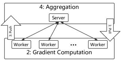
We focus on Stochastic Gradient Descent (SGD), and use the Parameter Server (PS) architecture (Li et al., 2014a, b) for distributed SGD. As illustrated in Figure 1, processes are composed of the server nodes and worker nodes. In each SGD iteration, the workers pull the latest model from the servers, estimate the gradients using the locally sampled training data, then push the gradient estimators to the servers. The servers aggregate the gradient estimators, and update the model by using the aggregated gradients.

Our approach, in a nutshell is the following. We treat each candidate gradient estimator as a suspect. We compute a score using a stochastic zero-order oracle. This ranking indicates how trustworthy the given worker is in that iteration. Then, we take the average over the several candidates with the highest scores. This allows us to tolerate a large number of incorrect gradients. We prove that the convergence is as fast as fault-free SGD. Further, the variance falls as the number of non-faulty workers increases.

To the best of our knowledge this paper is the first to theoretically and empirically study cases where a majority of workers are faulty for non-convex problems. In summary, our contributions are:

• A new approach for SGD with fault-tolerance, that works with an arbitrarily large number of faulty nodes as long as there is at least one non-faulty node.

• Theoretically, the proposed algorithm converges as fast as distributed synchronous SGD without faulty workers, with the same asymptotic time complexity.

• Experimental results validating that 1) existing majority-based robust algorithms may fail even when the number of faulty workers is lower than the majority, and 2) Zeno gracefully handles such cases.

• The effectiveness of Zeno also extends to the case where the workers use disjoint local data to train the model, i.e., the local training data are not identically distributed across different workers. Theoretical and experimental analysis is also provided in this case.

2 Related Work

Many approaches for improving failure tolerance are based on robust statistics. For instance, Chen et al. (2017); Su & Vaidya (2016a, b) use geometric median as the aggregation rule. Yin et al. (2018) establishes statistical error rates for marginal trimmed mean as the aggregation rule. Similar to these papers, our proposed algorithm also works under Byzantine settings.

There are also robust gradient aggregation rules that are not based on robust statistics. For example, Blanchard et al. (2017) propose Krum, which select the candidates with minimal local sum of Euclidean distances. DRACO (Chen et al., 2018) uses coding theory to ensure robustness.

Alistarh et al. (2018) proposes a fault-tolerant SGD variant different from the robust aggregation rules. The algorithm utilizes historical information, and achieves the optimal sample complexity.

Despite their differences, the existing majority-based methods for synchronous SGD (Blanchard et al., 2017; Chen et al., 2017; Yin et al., 2018; Su & Vaidya, 2016a; Alistarh et al., 2018) assume that the non-faulty workers dominate the entire set of workers. Thus, such algorithms can trim the outliers from the candidates. However, in real-world failures or attacks, there are no guarantees that the number of faulty workers can be bounded from above.

3 Model

We consider the following optimization problem:

$$\min_{x\in{\mathbb{R}}^{d}}F(x),$$

where $F(x)={\mathbb{E}}_{z\sim\mathcal{D}}[f(x;z)]$, $z$ is sampled from some unknown distribution $\mathcal{D}$, $d$ is the number of dimensions. We assume that there exists a minimizer of $F(x)$, which is denoted by $x^{*}$.

We solve this problem in a distributed manner with $m$ workers. In each iteration, each worker will sample $n$ independent and identically distributed (i.i.d.) data points from the distribution $\mathcal{D}$, and compute the gradient of the local empirical loss $F_{i}(x)=\frac{1}{n}\sum_{j=1}^{n}f(x;z^{i,j}),\forall i\in[m]$, where $z^{i,j}$ is the $j$th sampled data on the $i$th worker. The servers will collect and aggregate the gradients sent by the works, and update the model as follows:

$$x^{t+1}=x^{t}-\gamma^{t}{\tt Aggr}(\{g_{i}(x^{t}):i\in[m]\}),$$

where ${\tt Aggr}(\cdot)$ is an aggregation rule (e.g., averaging), and

$$g_{i}(x^{t})=\begin{cases}*&\mbox{$i$th worker is faulty},\\ \nabla F_{i}(x^{t})&\mbox{otherwise,}\end{cases}$$ (1)

where “$*$" represents arbitrary values.

Formally, we define the failure model in synchronous SGD as follows.

Definition 1.

(Failure Model). In the $t^{\mbox{th}}$ iteration, let $\{v_{i}^{t}:i\in[m]\}$ be i.i.d. random vectors in ${\mathbb{R}}^{d}$, where $v_{i}^{t}=\nabla F_{i}(x^{t})$. The set of correct vectors $\{v_{i}^{t}:i\in[m]\}$ is partially replaced by faulty vectors, which results in $\{\tilde{v}_{i}^{t}:i\in[m]\}$, where $\tilde{v}_{i}^{t}=g_{i}(x^{t})$ as defined in Equation (1). In other words, a correct/non-faulty gradient is $\nabla F_{i}(x^{t})$, while a faulty gradient, marked as “$*$", is assigned arbitrary value. We assume that $q$ out of $m$ vectors are faulty, where $q<m$. Furthermore, the indices of faulty workers can change across different iterations.

We observe that in the worst case, the failure model in Definition 1 is equivalent to the Byzantine failures introduced in Blanchard et al. (2017); Chen et al. (2017); Yin et al. (2018). In particular, if the failures are caused by attackers, the failure model includes the case where the attackers collude.

To help understand the failure model in synchronous SGD, we illustrate a toy example in Figure 2.

The notations used in this paper is summarized in Table 1.

Figure 2: A toy example of the failure model in synchronous SGD. There are $m=7$ candidate gradient estimators. The black dots represent the correct gradients, where $\tilde{v}_{i}=\nabla F_{i}(x^{t})$, $i\in[m-1]$. The red dot represents the faulty gradient, whose value (in the worst case) is $\tilde{v}_{m}=\epsilon\nabla F_{m}(x^{t})$, where $\epsilon<0$ is a large negative constant. The blue dashed circle represent the expectation of the true gradient $\nabla F(x^{t})$. Thus, the averaged gradient, which will be computed by the server, represented by the green dot, is far away from the true gradient, which is harmful to the model training.

Table 1: Notations

Notation	Description
$m$	Number of workers
$n$	Number of samples on each worker
$T$	Number of epochs
$[m]$	Set of integers $\{1,\ldots,m\}$
$q$	Number of faulty workers
$b$	Trim parameter of Zeno
$\gamma$	Learning rate
$\rho$	Regularization weight of Zeno
$n_{r}$	Batch size of Zeno
$\|\cdot\|$	All the norms in this paper are $l_{2}$-norms

4 Methodology

In contrast to the existing majority-based methods, we compute a score for each candidate gradient estimator by using the stochastic zero-order oracle. We rank each candidate gradient estimator based on the estimated descent of the loss function, and the magnitudes. Then, the algorithm aggregates the candidates with highest scores. The score roughly indicates how trustworthy each candidate is.

Definition 2.

(Stochastic Descendant Score) Denote $f_{r}(x)=\frac{1}{n_{r}}\sum_{i=1}^{n_{r}}f(x;z_{i})$, where $z_{i}$’s are i.i.d. samples drawn from $\mathcal{D}$, and $n_{r}$ is the batch size of $f_{r}(\cdot)$. ${\mathbb{E}}[f_{r}(x)]=F(x)$. For any update (gradient estimator) $u$, based on the current parameter $x$, learning rate $\gamma$, and a constant weight $\rho>0$, we define its stochastic descendant score as follows:

$$Score_{\gamma,\rho}(u,x)=f_{r}(x)-f_{r}(x-\gamma u)-\rho\|u\|^{2}.$$

The score defined in Definition 2 is composed of two parts: the estimated descendant of the loss function, and the magnitude of the update. The score increases when the estimated descendant of the loss function, $f_{r}(x)-f_{r}(x-\gamma\tilde{v}_{i})$, increases. The score decreases when the magnitude of the update, $\|\tilde{v}_{i}\|^{2}$, increases. Intuitively, the larger descendant suggests faster convergence, and the smaller magnitude suggests a smaller change. Even if a gradient is faulty, a smaller change makes it less harmful and easier to be cancelled by the correct gradients.

Using the score defined above, we establish the following suspicion-based aggregation rule. We ignore the index of iterations, $t$, for convenience.

Algorithm 1 Zeno

  Server

  Input: $\rho$ (defined in Definition 2), $b$ (defined in Definition 3)

  $x^{0}\leftarrow rand()$ {Initialization}

  for $t=1,\ldots,T$ do

     Broadcast $x^{t-1}$ to all the workers

     Wait until all the gradients $\{\tilde{v}_{i}^{t}:i\in[m]\}$ arrive

     Draw the samples for evaluating stochastic descendant score $f_{r}^{t}(\cdot)$ as defined in Definition 2

     Compute $\bar{\tilde{v}}^{t}={\tt Zeno}_{b}(\{\tilde{v}_{i}^{t}:i\in[m]\})$ as defined in Definition 3

     Update the parameter $x^{t}\leftarrow x^{t-1}-\gamma^{t}\bar{\tilde{v}}^{t}$

  end for

  Worker $i=1,\ldots,m$

  for $t=1,\ldots,T$ do

     Receive $x^{t-1}$ from the server

     Draw the samples, compute, and send the gradient $v_{i}^{t}=\nabla F_{i}^{t}(x^{t-1})$ to the server

  end for

Definition 3.

(Suspicion-based Aggregation) Assume that among the gradient estimators $\{\tilde{v}_{i}:i\in[m]\}$, $q$ elements are faulty, and $x$ is the current value of the parameters. We sort the sequence by the stochastic descendant score defined in Definition 2, which results in $\{\tilde{v}_{(i)}:i\in[m]\}$, where

$$Score_{\gamma,\rho}(\tilde{v}_{(1)},x)\geq\ldots\geq Score_{\gamma,\rho}(\tilde{v}_{(m)},x).$$

In other words, $\tilde{v}_{(i)}$ is the vector with the $i$th highest score in $\{\tilde{v}_{i}:i\in[m]\}$.

The proposed aggregation rule, Zeno, aggregates the gradient estimators by taking the average of the first $m-b$ elements in $\{\tilde{v}_{(i)}:i\in[m]\}$ (the gradient estimators with the $(m-b)$ highest scores), where $m>b\geq q$:

$${\tt Zeno}_{b}(\{\tilde{v}_{i}:i\in[m]\})=\frac{1}{m-b}\sum_{i=1}^{m-b}\tilde{v}_{(i)}.$$

Note that $z_{i}$’s (in Definition 2) are independently sampled in different iterations. Furthermore, in each iteration, $z_{i}$’s are sampled after the arrival of the candidate gradient estimators $\tilde{v}_{i}^{t}$ on the server. Since the faulty workers are not predictive, they cannot obtain the exact information of $f_{r}(\cdot)$, which means that the faulty gradients are independent of $f_{r}(\cdot)$, though the faulty workers can know ${\mathbb{E}}[f_{r}(\cdot)]$.

Using Zeno as the aggregation rule, the detailed distributed synchronous SGD is shown in Algorithm 1.

Figure 3: Zeno on loss surface contours. We use the notations in Definition 2 and 3. The black dot is the current parameter $x$. The arrows are the candidate updates $\{\tilde{v}_{i}:i\in[m]\}$. Red arrows are the incorrect updates. Green arrows are the correct updates. Taking $b=3$, Zeno filters out the 3 arrows pointing outside the black dashed circle. These 3 updates have the least descendant of the loss function, among all the updates. There are some incorrect updates (the red arrow) remaining inside the boundary. However, since they are bounded by the correct updates, the remaining incorrect updates are harmless.

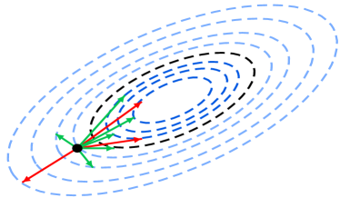
In Figure 3, we visualize the intuition underlying Zeno. It is illustrated that all the selected candidates (arrows pointing inside the black dashed circle) are bounded by at least one honest candidate. In other words, Zeno uses at least one honest candidate to establish a boundary (the black dashed circle), which filter out the potentially harmful candidates. The candidates inside the boundary are harmless, no matter they are actually faulty or not.

5 Theoretical Guarantees

In this section, we prove the convergence of synchronous SGD with Zeno as the aggregation rule under our failure model. We start with the assumptions required by the convergence guarantees. The two basic assumptions are the smoothness of the loss function, and the bounded variance of the (non-faulty) gradient estimators.

5.1 Assumptions

In this section, we highlight the necessary assumption for stochastic descendant score, followed by the assumptions for convergence guarantees.

Assumption 1.

(Unbiased evaluation) We assume that the stochastic loss function, $f_{r}(x)$, evaluated in the stochastic descendant score in Definition 2, is an unbiased estimator of the global loss function $F(x)$, i.e., ${\mathbb{E}}[f_{r}(x)]=F(x)$.

Assumption 2.

(Bounded Taylor’s Approximation) We assume that $f(x;z)$ has $L$-smoothness and $\mu$-lower-bounded Taylor’s approximation (also called $\mu$-weak convexity): $\left\langle\nabla f(x;z),y-x\right\rangle+\frac{\mu}{2}\|y-x\|^{2}\leq f(y;z)-f(x;z)\leq\left\langle\nabla f(x;z),y-x\right\rangle+\frac{L}{2}\|y-x\|^{2},$ where $\mu\leq L$, and $L>0$.

Note that Assumption 2 covers the case of non-convexity by taking $\mu<0$, non-strong convexity by taking $\mu=0$, and strong convexity by taking $\mu>0$.

Assumption 3.

(Bounded Variance) We assume that in any iteration, any correct gradient estimator $v_{i}=\nabla F_{i}(x)$ has the upper-bounded variance: ${\mathbb{E}}\left\|v_{i}-{\mathbb{E}}\left[v_{i}\right]\right\|^{2}\leq V.$ Furthermore, we assume that ${\mathbb{E}}\|v_{i}\|^{2}\leq G.$

In general, Assumption 3 bounds the variance and the second moment of the correct gradients of any sample loss function $f(x;z)$, $\forall z\sim\mathcal{D}$.

Remark 1.

Note that for the faulty gradients in our failure model, none of the assumptions above holds.

5.2 Convergence Guarantees

For general functions, including convex and non-convex functions, we provide the following convergence guarantee. The proof can be found in the appendix.

Theorem 1.

For $\forall x\in{\mathbb{R}}^{d}$, denote

$$\tilde{v}_{i}=\begin{cases}*&\mbox{$i$th worker is faulty},\\ \nabla F_{i}(x)&\mbox{otherwise,}\end{cases}$$

where $i\in[m]$, with ${\mathbb{E}}[\nabla F_{i}(x)]=\nabla F(x)$, and $\bar{\tilde{v}}={\tt Zeno}_{b}(\{\tilde{v}_{i}:i\in[m]\})$. Taking $\gamma\leq\frac{1}{L}$, $\rho=\frac{\beta\gamma^{2}}{2}$, and $\beta>\max(0,-\mu)$, we have

$${\mathbb{E}}\left[F(x-\gamma\bar{\tilde{v}})\right]-F(x)\leq-\frac{\gamma}{2}\|\nabla F(x)\|^{2}$$

$$\quad+\frac{\gamma(b-q+1)(m-q)V}{(m-b)^{2}}+\frac{(L+\beta)\gamma^{2}G}{2}.$$

Corollary 1.

Take $\gamma=\frac{1}{L\sqrt{T}}$, $\rho=\frac{\beta\gamma^{2}}{2}$, and $\beta>\max(0,-\mu)$. Using ${\tt Zeno}$, with ${\mathbb{E}}[\nabla F_{i}(x^{t})]=\nabla F(x^{t})$ for $\forall t\in\{0,\ldots,T\}$, after $T$ iterations, we have

$$\frac{\sum_{t=0}^{T-1}{\mathbb{E}}\|\nabla F(x^{t})\|^{2}}{T}$$

$$\leq\mathcal{O}\left(\frac{1}{\sqrt{T}}\right)+\mathcal{O}\left(\frac{(b-q+1)(m-q)}{(m-b)^{2}}\right).$$

Now, we consider a more general case, where each worker has a disjoint (non-identically distributed) local dataset for training, which results in non-identically distributed gradient estimators. The server is still aware of the the entire dataset. For example, in volunteer computing (Meeds et al., 2015; Miura & Harada, 2015), the server/coordinator can assign disjoint tasks/subsets of training data to the workers, while the server holds the entire training dataset. In this scenario, we have the following convergence guarantee.

Corollary 2.

Assume that

$$F(x)=\frac{1}{m}\sum_{i\in[m]}{\mathbb{E}}\left[F_{i}(x)\right],{\mathbb{E}}\left[F_{i}(x)\right]\neq{\mathbb{E}}\left[F_{j}(x)\right],$$

for $\forall i,j\in[m]$, $i\neq j$. For the stochastic descendant score, we have ${\mathbb{E}}\left[f_{r}(x)\right]=F(x)$. Assumption 1, 2, and 3 hold. Take $\gamma=\frac{1}{L\sqrt{T}}$, $\rho=\frac{\beta\gamma^{2}}{2}$, and $\beta>\max(0,-\mu)$. Using ${\tt Zeno}$, after $T$ iterations, we have

$$\frac{\sum_{t=0}^{T-1}{\mathbb{E}}\|\nabla F(x^{t})\|^{2}}{T}$$

$$\leq\mathcal{O}\left(\frac{1}{\sqrt{T}}\right)+\mathcal{O}\left(\frac{b}{m}\right)+\mathcal{O}\left(\frac{b^{2}(m-q)}{m^{2}(m-b)}\right).$$

These two corollaries tell us that when using Zeno as the aggregation rule, even if there are failures, the convergence rate can be as fast as fault-free distributed synchronous SGD. The variance decreases when the number of workers $m$ increases, or the estimated number of faulty workers $b$ decreases.

Remark 2.

There are two practical concerns for the proposed algorithm. First, by increasing the batch size of $f_{r}(\cdot)$ ($n_{r}$ in Definition 2), the stochastic descendant score will be potentially more stable. However, according to Theorem 1 and Corollary 1 and 2, the convergence rate is independent of the variance of $f_{r}$. Thus, theoretically we can use a single sample to evaluate the stochastic descendant score. Second, theoretically we need larger $\rho$ for non-convex problems. However, larger $\rho$ makes Zeno less sensitive to the descendant of the loss function, which potentially increases the risk of aggregating harmful candidates. In practice, we can use a small $\rho$ by assuming the local convexity of the loss functions.

5.3 Implementation Details: Time Complexity

Unlike the majority-based aggregation rules, the time complexity of Zeno is not trivial to analyze. Note that the convergence rate is independent of the variance of $f_{r}$, which means that we can use a single sample ($n_{r}=1$) to evaluate $f_{r}$ to achieve the same convergence rate. Furthermore, in general, when evaluating the loss function on a single sample, the time complexity is roughly linear to the number of parameters $d$. Thus, informally, the time complexity of Zeno is $\mathcal{O}(dm)$ for one iteration, which is the same as Mean and Median aggregation rules. For comparison, note that the time complexity of Krum is $\mathcal{O}(dm^{2})$.

(a) Top-1 accuracy on testing set, with $q=8$

(b) Cross entropy on training set, with $q=8$

Figure 4: Convergence on i.i.d. training data, without failures. Batch size on the workers is $100$. Batch size of Zeno is $n_{r}=4$. $\rho=0.0005$. $\gamma=0.1$. Each epoch has 25 iterations. Zeno performs similar to Mean.

(a) Top-1 accuracy on testing set, with $q=8$

(b) Cross entropy on training set, with $q=8$

(c) Top-1 accuracy on testing set, with $q=12$

(d) Cross entropy on training set, with $q=12$

Figure 5: Convergence on i.i.d. training data, with label-flipping failures. Batch size on the workers is $100$. Batch size of Zeno is $n_{r}=4$. $\rho=0.0005$. $\gamma=0.1$. Each epoch has 25 iterations. Zeno outperforms all the baselines, especially when $q=12$.

(a) Top-1 accuracy on testing set, with $q=8$

(b) Cross entropy on training set, with $q=8$

(c) Top-1 accuracy on testing set, with $q=12$

(d) Cross entropy on training set, with $q=12$

Figure 6: Convergence on i.i.d. training data, with bit-flipping failures. Batch size on the workers is $100$. Batch size of Zeno is $n_{r}=4$. $\rho=0.0005$. $\gamma=0.1$. Each epoch has 25 iterations. Zeno outperforms all the baselines, especially when $q=12$.

(a) Top-1 accuracy on testing set, with $q=8$

(b) Cross entropy on training set, with $q=8$

(c) Top-1 accuracy on testing set, with $q=12$

(d) Cross entropy on training set, with $q=12$

Figure 7: Convergence on disjoint (non-i.i.d.) training data, with label-flipping failures. Batch size on the workers is $100$. Batch size of Zeno is $n_{r}=4$. $\rho=0.0005$. $\gamma=0.05$. Each epoch has 25 iterations. Zeno outperforms all the baselines, especially when $q=12$.

(a) Top-1 accuracy on testing set, with $q=8$

(b) Cross entropy on training set, with $q=8$

Figure 8: Convergence on i.i.d. training data, with label-flipping failures, $q=8$. Batch size on the workers is $100$. $\gamma=0.1$. Each epoch has 25 iterations. $n_{r}$ is tuned.

6 Experiments

In this section, we evaluate the fault tolerance of the proposed algorithm. We summarize our results here:

• Compared to the baselines, Zeno shows better convergence with more faulty workers than non-faulty ones.

• Zeno is robust to the choices of the hyperparameters, including the Zeno batch size $n_{r}$, the weight $\rho$, and the number of trimmed elements $b$.

• Zeno also works when training with disjoint local data.

6.1 Datasets and Evaluation Metrics

We conduct experiments on benchmark CIFAR-10 image classification dataset (Krizhevsky & Hinton, 2009), which is composed of 50k images for training and 10k images for testing. We use convolutional neural network (CNN) with 4 convolutional layers followed by 1 fully connected layer. The detailed network architecture can be found in https://github.com/xcgoner/icml2019_zeno. In each experiment, we launch 20 worker processes. We repeat each experiment 10 times and take the average. We use top-1 accuracy on the testing set and the cross-entropy loss function on the training set as the evaluation metrics.

6.1.1 Baselines

We use the averaging without failures/attacks as the gold standard, which is referred to as Mean without failures. Note that this method is not affected by $b$ or $q$. The baseline aggregation rules are Mean, Median, and Krum as defined below.

Definition 4.

(Median (Yin et al., 2018)) We define the marginal median aggregation rule ${\tt Median}(\cdot)$ as $med={\tt Median}(\{\tilde{v}_{i}:i\in[m]\}),$ where for any $j\in[d]$, the $j$th dimension of $med$ is $med_{j}=median\left(\{(\tilde{v}_{1})_{j},\ldots,(\tilde{v}_{m})_{j}\}\right)$, $(\tilde{v}_{i})_{j}$ is the $j$th dimension of the vector $\tilde{v}_{i}$, $median(\cdot)$ is the one-dimensional median.

Definition 5.

(Krum (Blanchard et al., 2017))

$${\tt Krum}_{b}(\{\tilde{v}_{i}:i\in[m]\})=\tilde{v}_{k},\quad k=\mathop{\rm argmin}_{i\in[m]}\sum_{i\rightarrow j}\|\tilde{v}_{i}-\tilde{v}_{j}\|^{2},$$

where $i\rightarrow j$ is the indices of the $m-b-2$ nearest neighbours of $\tilde{v}_{i}$ in $\{\tilde{v}_{i}:i\in[m]\}$ measured by Euclidean distances.

Note that Krum requires $2b+2<m$. Thus, $b=8$ is the best we can take.

6.2 No Failure

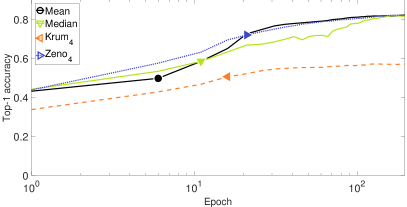
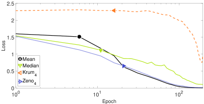
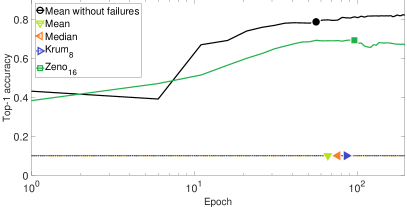
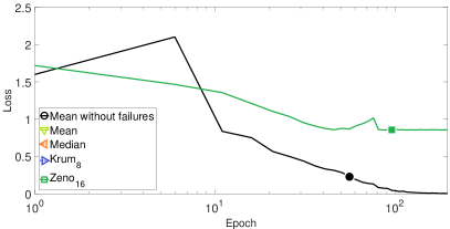
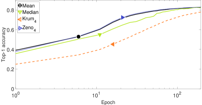
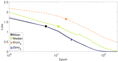
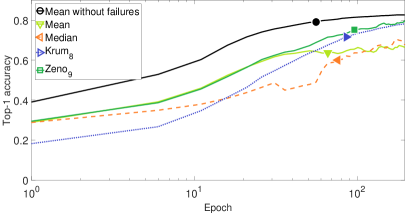
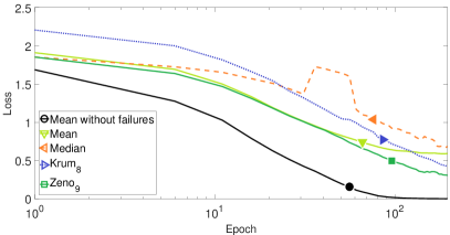
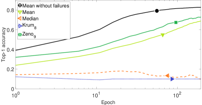
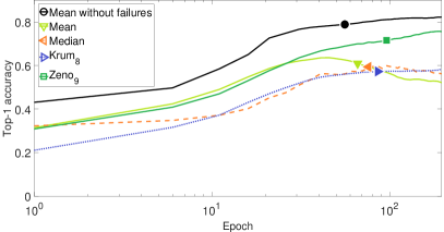
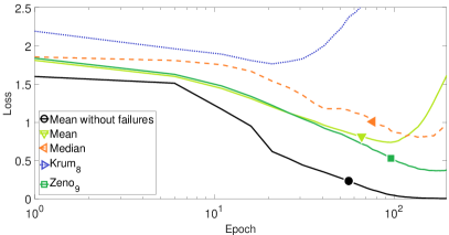
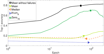
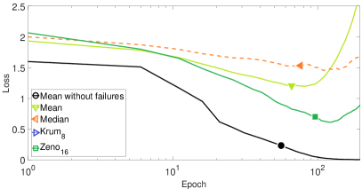
We first test the convergence when there are no failures. In all the experiments, we take the learning rate $\gamma=0.1$, worker batch size $100$, Zeno batch size $n_{r}=4$, and $\rho=0.0005$. Each worker computes the gradients on i.i.d. samples. For both Krum and Zeno, we take $b=4$. The result is shown in Figure 4. We can see that Zeno converges as fast as Mean. Krum converges slightly slower, but the convergence rate is acceptable.

6.3 Label-flipping Failure

In this section, we test the fault tolerance to label-flipping failures. When such failures happen, the workers compute the gradients based on the training data with “flipped" labels, i.e., any $label\in\{0,\ldots,9\}$, is replaced by $9-label$. Such failures/attacks can be caused by data poisoning or software failures.

In all the experiments, we take the learning rate $\gamma=0.1$, worker batch size $100$, Zeno batch size $n_{r}=4$, and $\rho=0.0005$. Each non-faulty worker computes the gradients on i.i.d. samples.

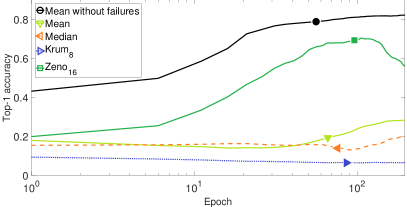
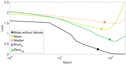
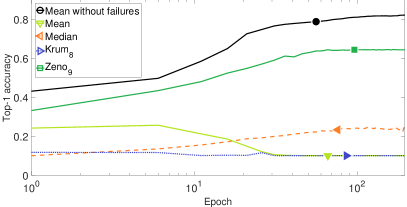
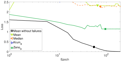
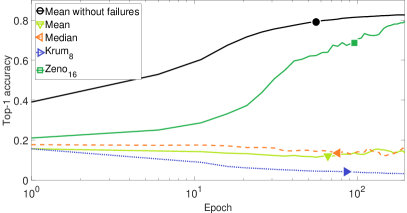
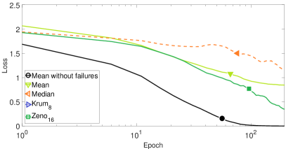
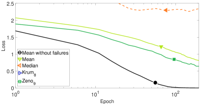
The result is shown in Figure 5. As expected, Zeno can tolerate more than half faulty gradients. When $q=8$, Zeno preforms similar to Krum. When $q=12$, Zeno preforms much better than the baselines. When there are faulty gradients, Zeno converges slower, but still has better convergence rates than the baselines.

6.4 Bit-flipping Failure

In this section, we test the fault tolerance to a more severe kind of failure. Here, the bits that control the sign of the floating numbers are flipped, e.g., due to some hardware failure. A faulty worker pushes the negative gradient instead of the true gradient to the servers. To make the failure even worse, one of the faulty gradients is copied to and overwrites the other faulty gradients, which means that all the faulty gradients have the same value.

In all the experiments, we take the learning rate $\gamma=0.1$, worker batch size $100$, Zeno batch size $n_{r}=4$, and $\rho=0.0005$. Each non-faulty worker computes the gradients on i.i.d. samples.

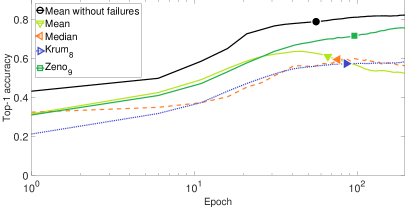
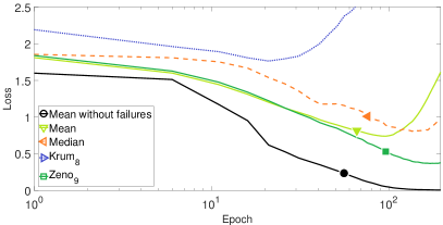
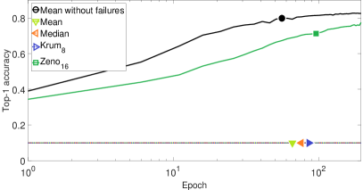
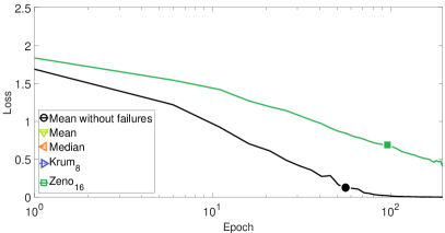
The result is shown in Figure 6. As expected, Zeno can tolerate more than half faulty gradients. Surprisingly, Mean performs well when $q=8$. We will discuss this phenomenon in Section 6.7. Zeno outperforms all the baselines. When $q=12$, Zeno is the only strategy which avoids catastrophic divergence. Zeno converges slower, but still has better convergence than the baselines.

6.5 Disjoint Local Training Data

In volunteer computing (Meeds et al., 2015; Miura & Harada, 2015), it is reasonable for the coordinator to assign disjoint tasks/datasets to different workers. As a result, each worker draws training samples from different datasets. The server is still aware of the entire dataset. We conduct experiments in such scenario, as discussed in Corollary 2. We test Zeno under label-flipping failures. The results are shown in Figure 7. Due to the non-i.i.d. setting, it is more difficult to distinguish faulty gradients from non-faulty ones. In such bad cases, Zeno can still make reasonable progress, while the baselines, especially Krum, performs much worse.

6.6 Hyperparameter Sensitivity

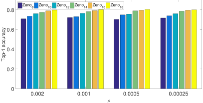
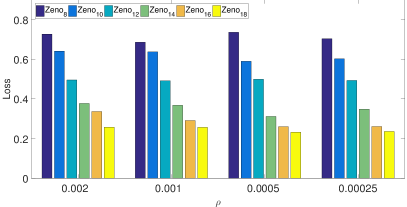
In Figure 8, we show the performance of Zeno with different batch size $n_{r}$. Larger $n_{r}$ improves the convergence, but the gap is not significant. $n_{r}=1$ still works. Zeno is also robust to different choices of the other hyperparameters $\rho$ and $b$. The experiments can be found in the appendix.

6.7 Discussion

An interesting observation is that, when $q=8$, Mean seems to have good performance, while it is not supposed to be fault-tolerant. The reason is that both label-flipping and bit-flipping failures do not change the magnitude of the gradients. When the number of faulty gradients $q$ is less than half, it is possible that the faulty gradients are cancelled out by the non-faulty ones. However, when the magnitude is enlarged, Mean will fail, as pointed out in Xie et al. (2018).

In general, we find that Zeno is more robust than the current state of the art. When the faulty workers dominate, Zeno is the only aggregator that converges in all experiments. When the correct workers dominate, Median can be an alternative with cheap computation.

The computational complexity of Zeno depends on the complexity of inference and the Zeno batch size $n_{r}$. These additional hyperparameters make direct comparison to standard methods more challenging. If we take the approximation that the computational complexity of inference is linear to the number of parameters, then we can roughly compare the time complexity to the baselines. Compared to Median, Zeno is computationally more expensive by the factor of $n_{r}=4$. However, compared to Krum, which requires $20\times 19/2=190$ times of $\mathcal{O}(d)$ operators, Zeno only needs $21\times 4=84$ times of $\mathcal{O}(d)$ operators. Furthermore, since the batch size on the workers is $100$, the computation required on the server is less than that of one worker, which does not cancel out the computational improvements due to data parallelism. The additional computation is the cost that we have to pay for better robustness.

Another interesting observation is that, although Krum is the state-of-the-art algorithm, it does not perform as well as expected under our designed failures. The reason is that Krum requires the assumption that $c\sigma<\|g\|$ for convergence, where $c$ is a general constant, $\sigma$ is the maximal variance of the gradients, and $g$ is the gradient. Note that $\|g\|\rightarrow 0$ when SGD converges to a critical point. Thus, such assumption is never guaranteed to be satisfied, if the variance is large. Furthermore, the better SGD converges, the less likely such assumption can be satisfied (more details of this issue can be found in Xie et al. (2019)).

7 Conclusion

We propose a novel aggregation rule for synchronous SGD, which requires a weak assumption that there is at least one honest worker. The algorithm has provable convergence. Our empirical results show good performance in practice. We will apply the proposed method to asynchronous SGD in future work.

Appendix

Appendix A Proofs

A.1 Preliminaries

We use the following lemma to bound the aggregated vectors.

Lemma 1.

(Bounded Score) Without loss of generality, we denote the $m-q$ correct elements in $\{\tilde{v}_{i}:i\in[m]\}$ as $\{v_{i}:i\in[m-q]\}$. Sorting the correct vectors by the stochastic descendant score, we obtain $\{v_{(i)}:i\in[m-q]\}$. Then, we have the following inequality:

$$Score_{\gamma,\rho}(\tilde{v}_{(i)},x)\geq Score_{\gamma,\rho}(v_{(i)},x),\forall i\in[m-q],$$

or, by flipping the signs on both sides, it is equivalent to

$$f_{r}(x-\gamma\tilde{v}_{(i)})-f_{r}(x)+\rho\|\tilde{v}_{(i)}\|^{2}\leq f_{r}(x-\gamma v_{(i)})-f_{r}(x)+\rho\|v_{(i)}\|^{2},\forall i\in[m-q],$$

Proof.

We prove the lemma by contradiction.

Assume that $Score_{\gamma,\rho}(\tilde{v}_{(i)},x)<Score_{\gamma,\rho}(v_{(i)},x)$. Thus, there are $i$ correct vectors having greater scores than $\tilde{v}_{(i)}$. However, because $\tilde{v}_{(i)}$ is the $i$th element in $\{\tilde{v}_{(i)}:i\in[m]\}$, there should be at most $i-1$ vectors having greater scores than it, which yields a contradiction. ∎

A.2 Convergence guarantees

For general non-strongly convex functions and non-convex functions, we provide the following convergence guarantees.

Theorem 1.

For $\forall x\in{\mathbb{R}}^{d}$, denote

$$\tilde{v}_{i}=\begin{cases}*&\mbox{$i$th worker is Byzantine},\\ \nabla F_{i}(x)&\mbox{otherwise,}\end{cases}$$

where $i\in[m]$, and $\bar{\tilde{v}}={\tt Zeno}_{b}(\{\tilde{v}_{i}:i\in[m]\})$. Taking $\gamma\leq\frac{1}{L}$, and $\rho=\frac{\beta\gamma^{2}}{2}$, where

$$\begin{cases}\beta=0,&\mbox{\quad if $\mu\geq 0$;}\\ \beta\geq|\mu|,&\mbox{\quad otherwise.}\end{cases}$$

we have

$${\mathbb{E}}\left[F(x-\gamma\bar{\tilde{v}})\right]-F(x)\leq-\frac{\gamma}{2}\|\nabla F(x)\|^{2}+\frac{\gamma(b-q+1)(m-q)V}{(m-b)^{2}}+\frac{(L+\beta)\gamma^{2}G}{2}.$$

Proof.

Without loss of generality, we denote the $m-q$ correct elements in $\{\tilde{v}_{i}:i\in[m]\}$ as $\{v_{i}:i\in[m-q]\}$, where ${\mathbb{E}}[v_{i}]=\nabla F(x)$. Sorting the correct vectors by the online descendant score, we obtain $\{v_{(i)}:i\in[m-q]\}$. We also sort $\tilde{v}_{i}$ by the online descendant score and obtain $\{\tilde{v}_{(i)}:i\in[m]\}$.

According to the definition, $\bar{\tilde{v}}={\tt Zeno}_{b}(\{\tilde{v}_{i}:i\in[m]\})=\frac{1}{m-b}\sum_{i=1}^{m-b}\tilde{v}_{(i)}$. Furthermore, we denote $\bar{v}=\frac{1}{m-b}\sum_{i=1}^{m-b}v_{(i)}$.

Using Assumption 2, we have

$$f_{r}(x-\gamma\tilde{v}_{(i)})\geq f_{r}(x-\gamma\bar{\tilde{v}})+\left\langle\nabla f_{r}(x-\gamma\bar{\tilde{v}}),\gamma(\bar{\tilde{v}}-\tilde{v}_{(i)})\right\rangle+\frac{\mu\gamma^{2}}{2}\|\bar{\tilde{v}}-\tilde{v}_{(i)}\|^{2},$$

for $\forall i\in[m-b]$.

By summing up, we have

$$\frac{1}{m-b}\sum_{i=1}^{m-b}f_{r}(x-\gamma\tilde{v}_{(i)})\geq f_{r}(x-\gamma\bar{\tilde{v}})+\frac{\mu\gamma^{2}}{2(m-b)}\sum_{i=1}^{m-b}\|\bar{\tilde{v}}-\tilde{v}_{(i)}\|^{2}.$$ (2)

Using Lemma 1, we have

$$f_{r}(x-\gamma\tilde{v}_{(i)})+\rho\|\tilde{v}_{(i)}\|^{2}\leq f_{r}(x-\gamma v_{(i)})+\rho\|v_{(i)}\|^{2},$$

for $\forall i\in[m-b]$.

Combined with Equation 2, we have

$$f_{r}(x-\gamma\bar{\tilde{v}})$$

$$\leq\frac{1}{m-b}\sum_{i=1}^{m-b}f_{r}(x-\gamma\tilde{v}_{(i)})-\frac{\mu\gamma^{2}}{2(m-b)}\sum_{i=1}^{m-b}\|\bar{\tilde{v}}-\tilde{v}_{(i)}\|^{2}$$

$$\leq\frac{1}{m-b}\sum_{i=1}^{m-b}f_{r}(x-\gamma v_{(i)})+\frac{\rho}{m-b}\sum_{i=1}^{m-b}\left[\|v_{(i)}\|^{2}-\|\tilde{v}_{(i)}\|^{2}\right]-\frac{\mu\gamma^{2}}{2(m-b)}\sum_{i=1}^{m-b}\|\bar{\tilde{v}}-\tilde{v}_{(i)}\|^{2}.$$

We take $\rho=\frac{\beta\gamma^{2}}{2}$, where

$$\begin{cases}\beta=0,&\mbox{\quad if $\mu\geq 0$;}\\ \beta\geq|\mu|,&\mbox{\quad otherwise.}\end{cases}$$

Thus, if $\mu\geq 0$, we have $\rho=0$, which implies that

$$\frac{\rho}{m-b}\sum_{i=1}^{m-b}\left[\|v_{(i)}\|^{2}-\|\tilde{v}_{(i)}\|^{2}\right]-\frac{\mu\gamma^{2}}{2(m-b)}\sum_{i=1}^{m-b}\|\bar{\tilde{v}}-\tilde{v}_{(i)}\|^{2}\leq\frac{\beta\gamma^{2}}{2(m-b)}\sum_{i=1}^{m-b}\|v_{(i)}\|^{2}.$$

Also, if $\mu<0$, since $\beta\geq-\mu$, we have

$$\frac{\rho}{m-b}\sum_{i=1}^{m-b}\left[\|v_{(i)}\|^{2}-\|\tilde{v}_{(i)}\|^{2}\right]-\frac{\mu\gamma^{2}}{2(m-b)}\sum_{i=1}^{m-b}\|\bar{\tilde{v}}-\tilde{v}_{(i)}\|^{2}$$

$$=\frac{\beta\gamma^{2}}{2(m-b)}\sum_{i=1}^{m-b}\left[\|v_{(i)}\|^{2}-\|\tilde{v}_{(i)}\|^{2}\right]-\frac{\mu\gamma^{2}}{2(m-b)}\sum_{i=1}^{m-b}\left[\|\tilde{v}_{(i)}\|^{2}-\|\bar{\tilde{v}}\|^{2}\right]$$

$$=\frac{\beta\gamma^{2}}{2(m-b)}\sum_{i=1}^{m-b}\|v_{(i)}\|^{2}+\frac{(-\beta-\mu)\gamma^{2}}{2(m-b)}\sum_{i=1}^{m-b}\|\tilde{v}_{(i)}\|^{2}+\frac{\mu\gamma^{2}}{2(m-b)}\sum_{i=1}^{m-b}\|\bar{\tilde{v}}\|^{2}$$

$$\leq\frac{\beta\gamma^{2}}{2(m-b)}\sum_{i=1}^{m-b}\|v_{(i)}\|^{2}.$$

Thus, we have

$$f_{r}(x-\gamma\bar{\tilde{v}})$$

$$\leq\frac{1}{m-b}\sum_{i=1}^{m-b}f_{r}(x-\gamma v_{(i)})+\frac{\rho}{m-b}\sum_{i=1}^{m-b}\left[\|v_{(i)}\|^{2}-\|\tilde{v}_{(i)}\|^{2}\right]-\frac{\mu\gamma^{2}}{2(m-b)}\sum_{i=1}^{m-b}\|\bar{\tilde{v}}-\tilde{v}_{(i)}\|^{2}$$

$$\leq\frac{1}{m-b}\sum_{i=1}^{m-b}f_{r}(x-\gamma v_{(i)})+\frac{\beta\gamma^{2}}{2(m-b)}\sum_{i=1}^{m-b}\|v_{(i)}\|^{2}.$$

Using the $L$-smoothness, we have

$$f_{r}(x-\gamma v_{(i)})\leq f_{r}(x-\gamma\bar{v})+\left\langle\nabla f_{r}(x-\gamma\bar{v}),\gamma(\bar{v}-v_{(i)})\right\rangle+\frac{L\gamma^{2}}{2}\|\bar{v}-v_{(i)}\|^{2},$$

for $\forall i\in[m-b]$. By summing up, we have

$$\frac{1}{m-b}\sum_{i=1}^{m-b}f_{r}(x-\gamma v_{(i)})$$

$$\leq f_{r}(x-\gamma\bar{v})+\frac{L\gamma^{2}}{2(m-b)}\sum_{i=1}^{m-b}\|\bar{v}-v_{(i)}\|^{2}$$

$$\leq f_{r}(x-\gamma\bar{v})+\frac{L\gamma^{2}}{2(m-b)}\sum_{i=1}^{m-b}\|v_{(i)}\|^{2}.$$

Thus, we have

$$f_{r}(x-\gamma\bar{\tilde{v}})$$

$$\leq\frac{1}{m-b}\sum_{i=1}^{m-b}f_{r}(x-\gamma v_{(i)})+\frac{\beta\gamma^{2}}{2(m-b)}\sum_{i=1}^{m-b}\|v_{(i)}\|^{2}$$

$$\leq f_{r}(x-\gamma\bar{v})+\frac{(L+\beta)\gamma^{2}}{2(m-b)}\sum_{i=1}^{m-b}\|v_{(i)}\|^{2}.$$

Again, using the $L$-smoothness and taking $\gamma\leq\frac{1}{L}$, we have

$$f_{r}(x-\gamma\bar{v})$$

$$\leq f_{r}(x)+\left\langle\nabla f_{r}(x),-\gamma\bar{v}\right\rangle+\frac{L\gamma^{2}}{2}\|\bar{v}\|^{2}$$

$$\leq f_{r}(x)+\left\langle\nabla f_{r}(x),-\gamma\bar{v}\right\rangle+\frac{\gamma}{2}\|\bar{v}\|^{2}$$

Thus, we have

$$f_{r}(x-\gamma\bar{\tilde{v}})-f_{r}(x)$$

$$\leq f_{r}(x-\gamma\bar{v})-f_{r}(x)+\frac{(L+\beta)\gamma^{2}}{2(m-b)}\sum_{i=1}^{m-b}\|v_{(i)}\|^{2}$$

$$\leq\left\langle\nabla f_{r}(x),-\gamma\bar{v}\right\rangle+\frac{\gamma}{2}\|\bar{v}\|^{2}+\frac{(L+\beta)\gamma^{2}}{2(m-b)}\sum_{i=1}^{m-b}\|v_{(i)}\|^{2}.$$

Conditional on $\tilde{v}_{(i)}$’s, taking expectation w.r.t. $f_{r}$ on both sides, we have

$$F(x-\gamma\bar{\tilde{v}})-F(x)$$

$$\leq\left\langle\nabla F(x),-\gamma\bar{v}\right\rangle+\frac{\gamma}{2}\|\bar{v}\|^{2}+\frac{(L+\beta)\gamma^{2}}{2(m-b)}\sum_{i=1}^{m-b}\|v_{(i)}\|^{2}$$

$$=-\frac{\gamma}{2}\|\nabla F(x)\|^{2}+\frac{\gamma}{2}\|\nabla F(x)-\bar{v}\|^{2}+\frac{(L+\beta)\gamma^{2}}{2(m-b)}\sum_{i=1}^{m-b}\|v_{(i)}\|^{2}.$$

Now, taking the expectation w.r.t. $\tilde{v}_{(i)}$’s on both sides and using ${\mathbb{E}}\|v_{(i)}\|^{2}\leq G$, we have

$${\mathbb{E}}\left[F(x-\gamma\bar{\tilde{v}})\right]-F(x)$$

$$\leq-\frac{\gamma}{2}\|\nabla F(x)\|^{2}+\frac{\gamma}{2}{\mathbb{E}}\|\nabla F(x)-\bar{v}\|^{2}+\frac{(L+\beta)\gamma^{2}}{2(m-b)}\sum_{i=1}^{m-b}{\mathbb{E}}\|v_{(i)}\|^{2}$$

$$\leq-\frac{\gamma}{2}\|\nabla F(x)\|^{2}+\frac{\gamma}{2}{\mathbb{E}}\|\nabla F(x)-\bar{v}\|^{2}+\frac{(L+\beta)\gamma^{2}G}{2}.$$

Now we just need to bound ${\mathbb{E}}\|\nabla F(x)-\bar{v}\|^{2}$. For convenience, we denote $g=\nabla F(x)$. Note that for arbitrary subset $\mathcal{S}\subseteq[m-q]$, $|\mathcal{S}|=m-b$, we have the following bound:

$${\mathbb{E}}\left\|\frac{\sum_{i\in\mathcal{S}}(v_{i}-g)}{m-b}\right\|^{2}$$

$$={\mathbb{E}}\left\|\frac{\sum_{i\in[m-q]}(v_{i}-g)-\sum_{i\notin\mathcal{S}}(v_{i}-g)}{m-b}\right\|^{2}$$

$$\leq 2{\mathbb{E}}\left\|\frac{\sum_{i\in[m-q]}(v_{i}-g)}{m-b}\right\|^{2}+2{\mathbb{E}}\left\|\frac{\sum_{i\notin\mathcal{S}}(v_{i}-g)}{m-b}\right\|^{2}$$

$$=\frac{2(m-q)^{2}}{(m-b)^{2}}{\mathbb{E}}\left\|\frac{\sum_{i\in[m-q]}(v_{i}-g)}{m-q}\right\|^{2}+\frac{2(b-q)^{2}}{(m-b)^{2}}{\mathbb{E}}\left\|\frac{\sum_{i\notin\mathcal{S}}(v_{i}-g)}{b-q}\right\|^{2}$$

$$\leq\frac{2(m-q)^{2}}{(m-b)^{2}}\frac{V}{m-q}+\frac{2(b-q)^{2}}{(m-b)^{2}}\frac{\sum_{i\in[m-q]}\|v_{i}-g\|^{2}}{b-q}$$

$$\leq\frac{2(m-q)^{2}}{(m-b)^{2}}\frac{V}{m-q}+\frac{2(b-q)^{2}}{(m-b)^{2}}\frac{(m-q)V}{b-q}$$

$$=\frac{2(b-q+1)(m-q)V}{(m-b)^{2}}.$$

Putting all the ingredients together, we obtain the desired result

$${\mathbb{E}}\left[F(x-\gamma\bar{\tilde{v}})\right]-F(x)$$

$$\leq-\frac{\gamma}{2}\|\nabla F(x)\|^{2}+\frac{\gamma(b-q+1)(m-q)V}{(m-b)^{2}}+\frac{(L+\beta)\gamma^{2}G}{2}.$$

∎

Corollary 1.

Take $\gamma=\frac{1}{L\sqrt{T}}$, and $\rho=\frac{\beta\gamma^{2}}{2}$, where $\beta$ is the same as in Theorem 1. Using ${\tt Zeno}$, after $T$ iterations, we have

$$\frac{\sum_{t=0}^{T-1}{\mathbb{E}}\|\nabla F(x^{t})\|^{2}}{T}$$

$$\leq\left[2L\left(F(x^{0})-F(x^{*})\right)+\frac{(L+\beta)G}{L}\right]\frac{1}{\sqrt{T}}+\frac{2(b-q+1)(m-q)V}{(m-b)^{2}}$$

$$=\mathcal{O}\left(\frac{1}{\sqrt{T}}\right)+\mathcal{O}\left(\frac{(b-q+1)(m-q)}{(m-b)^{2}}\right).$$

Proof.

Taking $x=x^{t}$, $x-\gamma{\tt Zeno}_{b}(\{\tilde{v}_{i}:i\in[m]\})=x^{t+1}$, using Theorem 1, we have

$${\mathbb{E}}\left[F(x^{t+1})\right]-F(x^{t})$$

$$\leq-\frac{\gamma}{2}\|\nabla F(x^{t})\|^{2}+\frac{\gamma(b-q+1)(m-q)V}{(m-b)^{2}}+\frac{(L+\beta)\gamma^{2}G}{2}.$$

By telescoping and taking total expectation, we have

$${\mathbb{E}}\left[F(x^{T})\right]-F(x^{0})$$

$$\leq-\frac{\gamma}{2}\sum_{t=0}^{T-1}{\mathbb{E}}\|\nabla F(x^{t})\|^{2}+\frac{\gamma(b-q+1)(m-q)VT}{(m-b)^{2}}+\frac{(L+\beta)\gamma^{2}GT}{2}.$$

Taking $\gamma=\frac{1}{L\sqrt{T}}$, we have

$$\frac{\sum_{t=0}^{T-1}{\mathbb{E}}\|\nabla F(x^{t})\|^{2}}{T}$$

$$\leq\frac{2L\left[F(x^{0})-F(x^{T})\right]}{\sqrt{T}}+\frac{2(b-q+1)(m-q)V}{(m-b)^{2}}+\frac{(L+\beta)G}{L\sqrt{T}}$$

$$\leq\frac{2L\left[F(x^{0})-F(x^{*})\right]}{\sqrt{T}}+\frac{2(b-q+1)(m-q)V}{(m-b)^{2}}+\frac{(L+\beta)G}{L\sqrt{T}}$$

$$=\mathcal{O}\left(\frac{1}{\sqrt{T}}\right)+\mathcal{O}\left(\frac{(b-q+1)(m-q)}{(m-b)^{2}}\right).$$

∎

Corollary 2.

Assume that

$$F(x)=\frac{1}{m}\sum_{i\in[m]}{\mathbb{E}}\left[F_{i}(x)\right],$$

and

$${\mathbb{E}}\left[F_{i}(x)\right]\neq{\mathbb{E}}\left[F_{j}(x)\right],$$

for $\forall i,j\in[m]$, $i\neq j$. For the stochastic descendant score, we still have ${\mathbb{E}}\left[f_{r}(x)\right]=F(x)$. Assumption 1, 2, and 3 still hold. Take $\gamma=\frac{1}{L\sqrt{T}}$, and $\rho=\frac{\beta\gamma^{2}}{2}$, where $\beta$ is the same as in Theorem 1. Using ${\tt Zeno}$, after $T$ iterations, we have

$$\frac{\sum_{t=0}^{T-1}{\mathbb{E}}\|\nabla F(x^{t})\|^{2}}{T}$$

$$\leq\frac{2L\left[F(x^{0})-F(x^{*})\right]}{\sqrt{T}}+\frac{4V}{m}+\frac{4bG}{m}+\frac{2b^{2}(m-q)G}{m^{2}(m-b)}+\frac{(L+\beta)G}{L\sqrt{T}}$$

$$=\mathcal{O}\left(\frac{1}{\sqrt{T}}\right)+\mathcal{O}\left(\frac{b}{m}\right)+\mathcal{O}\left(\frac{b^{2}(m-q)}{m^{2}(m-b)}\right).$$

Proof.

Similar to the proof of Theorem 1, we define $\bar{\tilde{v}}={\tt Zeno}_{b}(\{\tilde{v}_{i}:i\in[m]\})$. Thus, reusing the proof in Theorem 1, we have

$$F(x-\gamma\bar{\tilde{v}})-F(x)\leq-\frac{\gamma}{2}\|\nabla F(x)\|^{2}+\frac{\gamma}{2}\|\nabla F(x)-\bar{v}\|^{2}+\frac{(L+\beta)\gamma^{2}}{2(m-b)}\sum_{i=1}^{m-b}\|v_{(i)}\|^{2}.$$

Now, taking the expectation w.r.t. $\tilde{v}_{(i)}$’s on both sides and using ${\mathbb{E}}\|v_{(i)}\|^{2}\leq G$, we have

$${\mathbb{E}}\left[F(x-\gamma\bar{\tilde{v}})\right]-F(x)$$

$$\leq-\frac{\gamma}{2}\|\nabla F(x)\|^{2}+\frac{\gamma}{2}{\mathbb{E}}\|\nabla F(x)-\bar{v}\|^{2}+\frac{(L+\beta)\gamma^{2}}{2(m-b)}\sum_{i=1}^{m-b}{\mathbb{E}}\|v_{(i)}\|^{2}$$

$$\leq-\frac{\gamma}{2}\|\nabla F(x)\|^{2}+\frac{\gamma}{2}{\mathbb{E}}\|\nabla F(x)-\bar{v}\|^{2}+\frac{(L+\beta)\gamma^{2}G}{2}.$$

Now we just need to bound ${\mathbb{E}}\|\nabla F(x)-\bar{v}\|^{2}$. We define that $\mathcal{S}_{1}=\{\nabla F_{i}(x):i\in[m]\}\setminus\{v_{(i)}:i\in[m-b]\}$. Note that $|\mathcal{S}_{1}|=b$.

$${\mathbb{E}}\|\nabla F(x)-\bar{v}\|^{2}$$

$$={\mathbb{E}}\left\|\frac{1}{m}\sum_{i\in[m]}{\mathbb{E}}\left[\nabla F_{i}(x)\right]-\frac{1}{m-b}\sum_{i=1}^{m-b}v_{(i)}\right\|^{2}$$

$$\leq 2E\left\|\frac{1}{m}\sum_{i\in[m]}{\mathbb{E}}\left[\nabla F_{i}(x)\right]-\frac{1}{m}\sum_{i=1}^{m-b}v_{(i)}\right\|^{2}+2E\left\|\frac{1}{m}\sum_{i=1}^{m-b}v_{(i)}-\frac{1}{m-b}\sum_{i=1}^{m-b}v_{(i)}\right\|^{2}$$

$$\leq 4E\left\|\frac{1}{m}\sum_{i\in[m]}{\mathbb{E}}\left[\nabla F_{i}(x)\right]-\frac{1}{m}\sum_{i=1}^{m}\nabla F_{i}(x)\right\|^{2}+4E\left\|\frac{1}{m}\sum_{v\in\mathcal{S}_{1}}v\right\|^{2}+2E\left\|\frac{1}{m}\sum_{i=1}^{m-b}v_{(i)}-\frac{1}{m-b}\sum_{i=1}^{m-b}v_{(i)}\right\|^{2}$$

$$\leq\frac{4V}{m}+\frac{4b^{2}}{m^{2}}E\left\|\frac{1}{b}\sum_{v\in\mathcal{S}_{1}}v\right\|^{2}+2E\left\|\frac{1}{m}\sum_{i=1}^{m-b}v_{(i)}-\frac{1}{m-b}\sum_{i=1}^{m-b}v_{(i)}\right\|^{2}$$

$$\leq\frac{4V}{m}+\frac{4b^{2}}{m^{2}}\frac{mG}{b}+2\left[\frac{1}{m}-\frac{1}{m-b}\right]^{2}E\left\|\sum_{i=1}^{m-b}v_{(i)}\right\|^{2}$$

$$\leq\frac{4V}{m}+\frac{4bG}{m}+2\left[\frac{b}{m(m-b)}\right]^{2}(m-b)(m-q)G$$

$$\leq\frac{4V}{m}+\frac{4bG}{m}+\frac{2b^{2}(m-q)G}{m^{2}(m-b)}.$$

Thus, we have

$${\mathbb{E}}\left[F(x-\gamma\bar{\tilde{v}})\right]-F(x)$$

$$\leq-\frac{\gamma}{2}\|\nabla F(x)\|^{2}+\frac{\gamma}{2}\left[\frac{4V}{m}+\frac{4bG}{m}+\frac{2b^{2}(m-q)G}{m^{2}(m-b)}\right]+\frac{(L+\beta)\gamma^{2}G}{2}.$$

Follow the same procedure in Corollary 1, taking $\gamma=\frac{1}{L\sqrt{T}}$, we have

$$\frac{\sum_{t=0}^{T-1}{\mathbb{E}}\|\nabla F(x^{t})\|^{2}}{T}$$

$$\leq\frac{2L\left[F(x^{0})-F(x^{*})\right]}{\sqrt{T}}+\frac{4V}{m}+\frac{4bG}{m}+\frac{2b^{2}(m-q)G}{m^{2}(m-b)}+\frac{(L+\beta)G}{L\sqrt{T}}$$

$$=\mathcal{O}\left(\frac{1}{\sqrt{T}}\right)+\mathcal{O}\left(\frac{b}{m}\right)+\mathcal{O}\left(\frac{b^{2}(m-q)}{m^{2}(m-b)}\right).$$

∎

Appendix B Additional Experiments

(a) Top-1 accuracy on testing set, with $q=8$

(b) Cross entropy on training set, with $q=8$

Figure 9: Convergence on non-i.i.d. training data, without failures. Batch size on the workers is $100$. Batch size of Zeno is $n_{r}=4$. $\rho=0.0005$. Learning rate $\gamma=0.05$. Each epoch has 25 iterations.

(a) Top-1 accuracy on testing set, with $q=8$

(b) Cross entropy on training set, with $q=8$

(c) Top-1 accuracy on testing set, with $q=12$

(d) Cross entropy on training set, with $q=12$

Figure 10: Convergence on non-i.i.d. training data, with label-flipping failures. Batch size on the workers is $100$. Batch size of Zeno is $n_{r}=4$. $\rho=0.0005$. Learning rate $\gamma=0.05$. Each epoch has 25 iterations.

(a) Top-1 accuracy on testing set, with $q=8$

(b) Cross entropy on training set, with $q=8$

(c) Top-1 accuracy on testing set, with $q=12$

(d) Cross entropy on training set, with $q=12$

Figure 11: Convergence on non-i.i.d. training data, with bit-flipping failures. Batch size on the workers is $100$. Batch size of Zeno is $n_{r}=4$. $\rho=0.0005$. Learning rate $\gamma=0.05$. Each epoch has 25 iterations.

(a) Top-1 accuracy on testing set, with $q=8$

(b) Cross entropy on training set, with $q=8$

Figure 12: Convergence on i.i.d. training data, with label-flipping failures, $q=8$. Batch size on the workers is $100$. Batch size of Zeno is $n_{r}=4$. Learning rate $\gamma=0.1$. Each epoch has 25 iterations. $\rho$ and $b$ are tuned.

References

- Alistarh et al. (2018) Alistarh, D., Allen-Zhu, Z., and Li, J. Byzantine stochastic gradient descent. arXiv preprint arXiv:1803.08917, 2018.
- Blanchard et al. (2017) Blanchard, P., Guerraoui, R., Stainer, J., et al. Machine learning with adversaries: Byzantine tolerant gradient descent. In Advances in Neural Information Processing Systems, pp. 118–128, 2017.
- Chen et al. (2018) Chen, L., Wang, H., Charles, Z., and Papailiopoulos, D. Draco: Byzantine-resilient distributed training via redundant gradients. In International Conference on Machine Learning, pp. 902–911, 2018.
- Chen et al. (2017) Chen, Y., Su, L., and Xu, J. Distributed statistical machine learning in adversarial settings: Byzantine gradient descent. POMACS, 1:44:1–44:25, 2017.
- Feng et al. (2014) Feng, J., Xu, H., and Mannor, S. Distributed robust learning. arXiv preprint arXiv:1409.5937, 2014.
- Krizhevsky & Hinton (2009) Krizhevsky, A. and Hinton, G. Learning multiple layers of features from tiny images. 2009.
- Li et al. (2014a) Li, M., Andersen, D. G., Park, J. W., Smola, A. J., Ahmed, A., Josifovski, V., Long, J., Shekita, E. J., and Su, B.-Y. Scaling distributed machine learning with the parameter server. In OSDI, volume 14, pp. 583–598, 2014a.
- Li et al. (2014b) Li, M., Andersen, D. G., Smola, A. J., and Yu, K. Communication efficient distributed machine learning with the parameter server. In Advances in Neural Information Processing Systems, pp. 19–27, 2014b.
- Meeds et al. (2015) Meeds, E., Hendriks, R., al Faraby, S., Bruntink, M., and Welling, M. Mlitb: machine learning in the browser. PeerJ Computer Science, 1, 2015.
- Miura & Harada (2015) Miura, K. and Harada, T. Implementation of a practical distributed calculation system with browsers and javascript, and application to distributed deep learning. CoRR, abs/1503.05743, 2015.
- Su & Vaidya (2016a) Su, L. and Vaidya, N. H. Fault-tolerant multi-agent optimization: Optimal iterative distributed algorithms. In PODC, 2016a.
- Su & Vaidya (2016b) Su, L. and Vaidya, N. H. Defending non-bayesian learning against adversarial attacks. arXiv preprint arXiv:1606.08883, 2016b.
- Xie et al. (2018) Xie, C., Koyejo, O., and Gupta, I. Phocas: dimensional byzantine-resilient stochastic gradient descent. arXiv preprint arXiv:1805.09682, 2018.
- Xie et al. (2019) Xie, C., Koyejo, S., and Gupta, I. Fall of empires: Breaking byzantine-tolerant sgd by inner product manipulation. arXiv preprint arXiv:1903.03936, 2019.
- Yin et al. (2018) Yin, D., Chen, Y., Ramchandran, K., and Bartlett, P. Byzantine-robust distributed learning: Towards optimal statistical rates. arXiv preprint arXiv:1803.01498, 2018.