Myopic Bayesian Design of Experiments via
Posterior Sampling and Probabilistic Programming

Abstract

We design a new myopic strategy for a wide class of sequential design of experiment (DOE) problems, where the goal is to collect data in order to to fulfil a certain problem specific goal. Our approach, Myopic Posterior Sampling (MPS), is inspired by the classical posterior (Thompson) sampling algorithm for multi-armed bandits and leverages the flexibility of probabilistic programming and approximate Bayesian inference to address a broad set of problems. Empirically, this general-purpose strategy is competitive with more specialised methods in a wide array of DOE tasks, and more importantly, enables addressing complex DOE goals where no existing method seems applicable. On the theoretical side, we leverage ideas from adaptive submodularity and reinforcement learning to derive conditions under which MPS achieves sublinear regret against natural benchmark policies.

1 Introduction

Many real world problems fall into the design of experiments (DOE) framework, where one wishes to design a sequence of experiments and collect data so as to achieve a desired goal. For example, in electrolyte design for batteries, a chemist would like to conduct experiments that measure battery conductivity in order to identify an electrolyte that maximises the conductivity. On a different day, she would like to conduct experiments with different electrolyte designs to learn how the viscosity of the electrolyte changes with design. These two tasks, black-box optimisation and active learning, fall under the umbrella of DOE and are pervasive in industrial and scientific applications.

While several methods exist for specific DOE tasks, real world problems are broad and complex, and specialised approaches have limited applicability. Continuing with the electrolyte design example, the chemist can typically measure both conductivity and viscosity with a single experiment [18]. Since such experiments are expensive, it is wasteful to first perform a set of experiments to optimise conductivity and then a fresh set to learn viscosity. It is preferable to design a single set of experiments that simultaneously achieves both goals. Another example is metallurgy, where one wishes to conduct experiments to identify phase transitions in an alloy as the composition of metals changes [4]. Here and elsewhere, both the model and the goal of the experimenter are very application specific and cannot be simply shoe-horned into formulations like black-box optimisation or active learning.

To address these varied applications, we develop a general and flexible framework for DOE, where a practitioner may incorporate domain expertise about the system via a Bayesian model and specify her desired goal via a penalty function $\lambda$, which can depend on unknown system characteristics and the data collected during the DOE process. We then develop a myopic strategy for DOE, inspired by posterior (Thompson) sampling for multi-armed bandits [50]. Our approach has two key advantages. First, the Bayesian formulation allows us to exploit advances in probabilistic programming [5, 51] to incorporate domain expertise without introducing complexity. Since experiments are typically extremely expensive in applications, incorporating domain expertise is essential to achieving the desired goal in few experiments. Probabilisitic programming offers an elegant method to do so. Second, our myopic/greedy strategy is simple and computationally attractive in comparison with policies that engage in long-term planning. Nevertheless, borrowing ideas from submodular optimisation and reinforcement learning, we derive natural conditions under which our myopic policy is competitive with the globally optimal one. Our specific contributions are:

1. We propose a flexible framework for DOE that allows a practitioner to describe their system (via a probabilistic model) and specify their goal (via a penalty function). We also derive an algorithm, Myopic Posterior Sampling (MPS), for this setting.

2. We implement MPS using probabilistic programming and demonstrate that it performs favourably in a variety of synthetic and real world DOE problems. Despite our general formulation, MPS is competitive with specialised methods designed for particular problems.

3. In our theoretical analysis, we explore conditions under which MPS, which learns about the system over time, is competitive with myopic and globally optimal strategies that have full knowledge of the system.

Related work: The classical results for (sequential) DOE focus on discrete settings [42, 11] or linear models [14], which enable a more detailed characterization and refined analysis than we provide. More recent work in the bandit community studies more complex non-linear models [2, 47, 48], but ignores temporal dependencies that arise in applications. We focus on posterior sampling (PS) [50] as the bandit algorithm, since it has proven to be quite general and admits a clean Bayesian analysis [44]. PS has been studied in a number of bandit settings [22, 33, 30], and some episodic RL problems [40, 38, 21], where the agent is allowed to restart. In contrast, here we study PS on a single long trajectory with no restarts.

Myopic/greedy policies are known to be near-optimal for sequential decision making problems with adaptive submodularity [19], which generalizes submodularity and formalizes a diminishing returns property. Adaptive submodularity has been used for several DOE setups including active learning [20, 8, 10] and detection [9], but these papers focus on characterizing applications that admit near-optimal greedy strategies, and do not address the question of learning such a policy. As such, these results are complementary to ours: adaptive submodularity controls the approximation error (the difference between myopic- and globally-optimal strategies, both of which know the penalty $\lambda$), while we control the estimation error (how close our learned policy is to the myopic optimal policy that knows $\lambda$). As we show in Theorem 3, with adaptive submodularity, MPS can also compete with the globally optimal non-myopic policy. Prior results for learning in (adaptive) submodular environments are episodic and allow restarts [15, 16], which is unnatural in the DOE setup.

Our formulation can also be cast as reinforcement learning since at each round the agent makes a decision (what experiment to perform) with the goal of minimizing a long-term cost (the penalty function). One goal of our work is to understand when myopic “bandit-like" strategies perform well in reinforcement learning environments with long-term temporal dependencies. There are two main differences with prior work [34, 49, 28, 40, 38]: first, we make no explicit assumptions about the complexity of the state and action space, instead placing assumptions on the penalty (reward) structure and optimal policy, which is a better fit for our applications. More importantly, in our setup, the true penalty is never revealed to the agent, and instead it receives side-observations that provide information about an underlying parameter governing the environment. Lastly, our focus is on understanding when myopic strategies have reasonable performance rather than on achieving global optimality; it may be possible and interesting to extend these results to the general RL setting.

2 Set up and Method

Let $\Theta$ denote a parameter space, $\mathcal{X}$ an action space, and $\mathcal{Y}$ an outcome space. We consider a Bayesian setting where a true parameter $\theta_{\star}\in\Theta$ is drawn from a prior distribution $\rho_{0}$. A decision maker repeatedly chooses an action $X\in\mathcal{X}$, conducts an experiment at $X$, and observes the outcome $Y_{{X}}\in\mathcal{Y}$. We assume $Y_{{X}}$ is drawn from a likelihood $\mathbb{P}(\cdot|X,\theta_{\star})$, with known distributional form. This process proceeds for $n$ rounds, resulting in a data sequence $D_{n}=\{(X_{j},Y_{{X_{j}}})\}_{j=1}^{n}$, which is an ordered multi-set of action-observation pairs. With $\mathcal{D}$ denoting the set of all possible data sequences, the goal is to minimise a penalty function $\lambda:\Theta\times\mathcal{D}\rightarrow[0,1]$. In particular, we focus on the following two criteria, depending on the application:

$${\rm\bf(a)}\;\;\Lambda(\theta_{\star},{D}_{n})=\sum_{t=1}^{n}\lambda(\theta_{\star},{D}_{t})\hskip 72.26999pt{\rm\bf(b)}\;\;\lambda(\theta_{\star},{D}_{n}),$$ (1)

Here, ${D}_{t}=\{(X_{j},Y_{{X_{j}}})\}_{j=1}^{t}$ denotes the prefix of length $t$ of the data sequence ${D}_{n}$ collected by the decision maker. The former notion is the cumulative sum of all penalties, while the latter corresponds just to the penalty once all experiments have been completed. Note that since the penalty function depends on the unknown true parameter $\theta_{\star}$, the decision maker cannot compute the penalty during the data collection process, and instead must infer the penalty from observations in order to minimise it. This is a key distinction from existing work on reinforcement learning and sequential optimisation, and one of the new challenges in our setting.

Example 1.

A motivating example is Bayesian active learning [20, 10]. Here, actions $X$ correspond to data points while $Y_{{X}}$ is the label and $\mathbb{P}(y|x,\theta)$ specifies an assumed discriminative model. We may set $\lambda(\theta,{D}_{n})=\|\tau(\theta)-\hat{\tau}({D}_{n})\|_{2}^{2}$ where $\tau$ is a parameter of interest and $\hat{\tau}$ is a predetermined estimator (e.g. maximum likelihood or maximum a posteriori). The true penalty $\lambda(\theta_{\star},{D}_{n})$ is not available to the decision maker since it requires knowing $\tau(\theta_{\star})$.

Notation:

For each $t\in\mathbb{N}$, let $\mathcal{D}_{t}=\{\{(X_{j},Y_{{X_{j}}})\}_{j=1}^{t}:X_{j}\in\mathcal{X},Y_{{X_{j}}}\in\mathcal{Y}\}$ denote the set of all data sequences of length $t$, so that $\mathcal{D}=\bigcup_{t\in\mathbb{N}}\mathcal{D}_{t}$. We use $|D|$ to denote the length of a data sequence and $D\uplus D^{\prime}$ for the concatenation of two sequences. $D\prec D^{\prime}$ and $D^{\prime}\succ D$ both equivalently denote that $D$ is a prefix of $D^{\prime}$. Given a data sequence $D_{t}$, we use $D_{t^{\prime}}$ for $t^{\prime}<t$ to denote the prefix of the first $t^{\prime}$ action-observation pairs.

A policy for experiment design chooses a sequence of actions $\{X_{j}\}_{j\in\mathbb{N}}$ based on past actions and observations. In particular, for a randomised policy $\pi=\{\pi_{j}\}_{j\in\mathbb{N}}$, at time $t$, an action is drawn from $\pi_{t}(D_{t-1})=\mathbb{P}(X_{t}\in\cdot|D_{t-1})$. Two policies that will appear frequently in the sequel are $\pi_{\rm M}^{\star}$ and $\pi_{\rm G}^{\star}$, both of which operate with knowledge of $\theta_{\star}$. $\pi_{\rm M}^{\star}$ is the myopic optimal policy, which, from every data sequence ${D}_{t}$ chooses the action $X$ minimizing the expected penalty at the next step: $\mathbb{E}[\lambda(\theta_{\star},{D}_{t}\uplus\{(X,Y_{{X}})\})|\theta_{\star},{D}_{t}]$. On the other hand $\pi_{\rm G}^{\star}$ is the non-myopic, globally optimal adaptive policy, which in state ${D}_{t}$ with $n-t$ steps to go chooses the action to minimise the expected long-term penalty: $\mathbb{E}[\lambda(\theta_{\star},{D}_{t}\uplus\{(X,Y_{{X}})\}\uplus{D}_{t+2:n})\mid\pi_{\rm G}^{\star},\theta_{\star},{D}_{t}]$. Observe that $\pi_{\rm G}^{\star}$ may depend on the time horizon $n$ while $\pi_{\rm M}^{\star}$ does not.

Design of Experiments via Posterior Sampling

We present a simple and intuitive myopic strategy that aims to minimise $\lambda$ based on the posterior of the data collected so far. For this, first define the expected look-ahead penalty $\lambda^{+}:\Theta\times\mathcal{D}\times\mathcal{X}\rightarrow[0,1]$ to be the expected penalty at the next time step if $\theta\in\Theta$ were the true parameter and we were to take action $x\in\mathcal{X}$. Precisely, for a data sequence $D$,

$$\lambda^{+}(\theta,D,x)\;=\;\mathbb{E}_{Y_{{x}}\sim\mathbb{P}(Y|x,\theta)}\Big{[}\lambda_{t}\big{(}\theta,\,D\uplus\{(x,Y_{{x}})\}\,\big{)}\Big{]}.$$ (2)

The proposed policy, presented in Algorithm 1, is called MPS (Myopic Posterior Sampling) and is denoted $\pi_{\rm M}^{{{}^{{}_{\rm PS}}}}$. At time step $t$, it first samples a parameter value $\theta$ from the posterior for $\theta_{\star}$ conditioned on the data, i.e. $\theta\sim\mathbb{P}(\theta_{\star}|{D}_{t-1})$. Then, it chooses the action $X_{t}$ that is expected to minimise the penalty $\lambda$ by pretending that $\theta$ was the true parameter. It performs the experiment at $X_{t}$, collects the observation $Y_{{X_{t}}}$, and proceeds to the next time step.

0:  Prior $\rho_{0}$ for $\theta_{\star}$, Conditional distribution $\mathbb{P}(Y|X,\theta)$.

1:  ${D}_{0}\leftarrow\varnothing$.

2:  for $t=1,2,\dots$ do

3:     Sample $\theta\sim\rho_{t-1}\equiv\mathbb{P}(\theta_{\star}|{D}_{t-1})$.

4:     Choose $X_{t}=\mathop{\mathrm{argmin}}_{x\in\mathcal{X}}\lambda^{+}_{t-1}(\theta,{D}_{t-1},x)$.

5:     $Y_{{X_{t}}}\leftarrow$ conduct experiment at $X_{t}$.

6:     Set ${D}_{t}\leftarrow{D}_{t-1}\cup\{(X_{t},Y_{{X_{t}}})\}$.

7:  end for

Algorithm 1  MPS ($\pi_{\rm M}^{{{}^{{}_{\rm PS}}}}$)

Computational considerations: It is worth pointing out some of the computational considerations in Algorithm 1. First, sampling from the posterior for $\theta_{\star}$ in step 3 might be difficult, especially in complex Bayesian models. Fortunately however, the field of Bayesian inference has made great strides in the recent past seeing the development of fast techniques for approximate inference methods such as MCMC or variational inference [36, 25]. Moreover, today we have efficient probabilistic programming tools [5, 51] that allow a practitioner to intuitively incorporate domain expertise via a prior and obtain the posterior given data. Secondly, the minimisation of the look ahead penalty in step 4 can also be non-trivial, especially since it might involve empirically computing the expectation in (2). This is similar to existing work in Bayesian optimisation which assume access to such an optimisation oracle [47, 3]. That said, in many practical settings where experiments are financially expensive and can take several hours, these considerations are less critical.

Despite these concerns, it is worth mentioning that myopic strategies are still computationally far more attractive than policies which try to behave globally optimally. For example, extending MPS to a $k$ step look-ahead might involve an optimisation over $\mathcal{X}^{k}$ in step 4 of Algorithm 1 which might be impractical for large values of $k$ except in the most trivial settings.

Specification of the prior: In real world applications, the prior could be specified by a domain expert with knowledge of the given DOE problem. In some instances, the expert may only be able to specify the relations between the various variables involved. In such cases, one can specify the parametric form for the prior, and learn the parameters of the prior in an adaptive data dependent fashion using maximum likelihood and/or maximum a posteriori techniques [46]. While we adopt both approaches in our experiments, we assume a fixed prior in our theoretical analysis.

3 Examples & Experiments

In this section, we give some concrete examples of DOE problems that can be specified by a penalty function $\lambda$ and present experimental results for these settings. We compare $\pi_{\rm M}^{{{}^{{}_{\rm PS}}}}$ to random sampling (RAND), the myopically optimal policy $\pi_{\rm M}^{\star}$ which assumes access to $\theta_{\star}$, and in some cases to specialised methods developed for the particular problem. In the interest of aligning our experiments with our theoretical analysis, we compare methods on both criteria in (1), although in these applications, the final penalty $\lambda(\theta_{\star},{D}_{n})$ is more important than the cumulative one $\Lambda(\theta_{\star},{D}_{n})$.

High-level Takeaways:

Despite being a quite general, $\pi_{\rm M}^{{{}^{{}_{\rm PS}}}}$ outperforms, or performs as well as, specialised methods. $\pi_{\rm M}^{{{}^{{}_{\rm PS}}}}$ is competitive, but slightly worse than the non-realisable $\pi_{\rm M}^{\star}$. Finally $\pi_{\rm M}^{{{}^{{}_{\rm PS}}}}$ enables effective DOE in complex settings where no prior methods seem applicable.

Implementation details:

One of the experiments in Section 3.1 admits analytical computation of the posterior. In all other experiments, we use the Edward probabilistic programming framework [51]. We use variational inference to approximate the posterior, and then draw a sample from this approximation. The look-ahead penalty (2) is computed empirically by drawing $50$ samples from $Y|X,\theta$ for the sampled $\theta$. We minimise $\lambda^{+}$ by evaluating it on a fine grid and choosing the maximum. We use grid sizes $100$, $2500$, and $27000$ respectively for one, two and three dimensional domains $\mathcal{X}$.

3.1 Active Learning

Problem: As described previously, we wish to learn some parameter $\tau_{\star}=\tau(\theta_{\star})$ which is a function of the true parameter $\theta_{\star}$. Each time we query some $X\in\mathcal{X}$, we see a noisy observation (label) $Y\sim\mathbb{P}(Y|X,\theta_{\star})$. We conduct two synthetic experiments in this setting. We use $\|\tau_{\star}-\hat{\tau}({D}_{n})\|_{2}^{2}$ as the penalty where $\hat{\tau}$ is a regularised maximum likelihood estimator. In addition to RAND and $\pi_{\rm M}^{\star}$, we compare $\pi_{\rm M}^{{{}^{{}_{\rm PS}}}}$ to the ActiveSelect method of Chaudhuri et al. [7].

Experiment 1: We use the following logistic regression model: $Y_{{x}}|x,\theta\sim\mathcal{N}(f_{{\theta}}(x),\eta^{2})$ where $f_{{\theta}}(x)=\frac{a}{1+e^{b(x-c)}}$. The true parameter is $\theta_{\star}=(a,b,c,\eta^{2})$ and our goal is to estimate $\tau_{\star}=(a,b,c)$. The MLE is computed via gradient ascent on the log likelihood. In our experiments, we used $a=2.1,b=7,c=6$ and $\eta^{2}=0.01$ as $\theta_{\star}$. We used normal priors $\mathcal{N}(2,1)$, $\mathcal{N}(5,3)$ and $\mathcal{N}(5,3)$ for $a,b,c$ respectively and an inverse gamma ${\rm IG}(20,1)$ prior for $\eta^{2}$. As the action space, we used $\mathcal{X}=[0,10]$. For variational inference, we used a normal approximation for the posterior for $a,b,c$ and an inverse gamma approximation for $\eta^{2}$. The results are given in the first column of Figure 1.

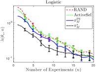
(a)

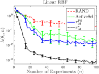
(b)

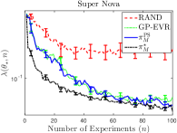
(c)

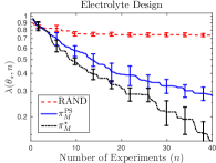
(d)

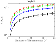
(e)

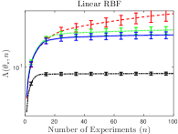
(f)

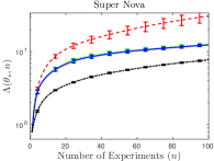
(g)

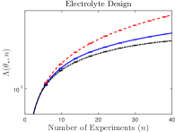
(h)

Figure 1: Results on the experiments. In all figures, the $x$ axis is the number of experiments $n$. In the top four figures, the $y$ axis is the final penalty $\lambda(\theta_{\star},n)$ at the $n$${}^{\textrm{th}}$ iteration and in the bottom figures, it is the cumulative penalty $\Lambda(\theta_{\star},n)$. Lower is better in both cases. The first two columns are the active learning problems (Sec. 3.1), the third is the posterior estimation problem (Sec. 3.2), and the fourth is the combined objective problem (Sec. 3.3). All curves were averaged over at least 10 runs, and error bars indicate one standard error.

Experiment 2: In the second example, we use the following linear regression model: $Y_{{x}}|x,\theta\sim\mathcal{N}(f_{{\theta}}(x),0.01)$ where $f_{{\theta}}(x)=\sum_{i=1}^{16}\theta_{*i}\phi(x-c_{i})$. Here, $\phi(v)=\frac{1}{\sqrt{0.2\pi}}e^{-5\|v\|_{2}^{2}}$ and the points $c_{1},\dots,c_{16}$ were arranged in a $4\times 4$ grid within $[0,1]^{2}$. We set $\theta_{*i}=g(c_{i})$, with $g(v)=\sin(3.9\pi((v_{1}-0.1)^{2}+v_{2}+0.1))$. Our goal is to estimate $\tau_{\star}=\theta_{\star}$. As the action space, we used $\mathcal{X}=[0,1]^{2}$. The posterior for $\theta_{\star}$ was calculated in closed form using a normal distribution $\mathcal{N}(0,I_{16})$ as the prior. The results are given in the second column of Figure 1.

3.2 Posterior Estimation & Active Regression

Problem: Consider estimating a non-parametric function $f_{{\theta_{\star}}}$, which is known to be uniformly smooth. An action $x\in\mathcal{X}$ is a query to the function $f$, upon which we observe $Y_{{x}}=f_{{\theta_{\star}}}(x)+\epsilon$, where $\mathbb{E}[\epsilon]=0$. If the goal is to learn $f_{{\theta_{\star}}}$ uniformly well in $L^{2}$ error, i.e. with penalty $\|f_{{\theta_{\star}}}-\hat{f}({D}_{n})\|^{2}$, adaptive techniques may not perform significantly better than non-adaptive ones [52]. However, if our penalty was $\lambda(\theta_{\star},{D}_{n})=\|\sigma(f_{{\theta_{\star}}})-\sigma(\hat{f}({D}_{n}))\|^{2}$ for some monotone super-linear transformation $\sigma$, then adaptive techniques may do better by requesting more evaluations at regions with high $f_{{\theta_{\star}}}$ value. This is because, $\lambda(\theta_{\star},{D}_{n})$ is more sensitive to such regions due to the transformation $\sigma$.

A particularly pertinent instance of this formulation arises in astrophysical applications where one wishes to estimate the posterior distribution of cosmological parameters, given some astronomical data $Q$ [41]. Here, an astrophysicist specifies a prior $\Xi$ over the cosmological parameters $Z\in\mathcal{X}$, and the likelihood of the data for a given choice of the cosmological parameters $x\in\mathcal{X}$ is computed via an expensive astrophysical simulation. The prior and the likelihood gives rise to an unknown log joint density $f_{{\theta_{\star}}}$ defined on $\mathcal{X}$, and the goal is to estimate the the joint density $p(Z=x,Q)=\exp(f_{{\theta_{\star}}}(x))$ so that we can perform posterior inference. Adopting assumptions from prior work [29] we model $f_{{\theta_{\star}}}$ as a Gaussian process, which is reasonable since we expect a log density to be smoother than the density itself. As we wish to estimate the joint density, $\lambda$ takes the above form with $\sigma=\exp$.

Experiment 3: We use data on Type I-a supernova from Davis et al [13]. We wish to estimate the posterior over the Hubble constant $H\in(60,80)$, the dark matter fraction $\Omega_{M}\in(0,1)$ and the dark energy fraction $\Omega_{E}\in(0,1)$, which constitute our three dimensional action space $\mathcal{X}$. The likelihood is computed via the Robertson-Walker metric. In addition to $\pi_{\rm M}^{\star}$ and RAND, we compare $\pi_{\rm M}^{{{}^{{}_{\rm PS}}}}$ to Gaussian process based exponentiated variance reduction (GP-EVR) [29] which was specifically designed for this setting. We evaluate the penalty via numerical integration. The results are presented in the third column of Figure 1.

3.3 Combined and Customised Objectives

Problem: In many real world problems, one needs to design experiments with multiple goals. For example, an experiment might evaluate multiple objectives, and the task might be to optimise some of them, while learning the parameters for another. Classical methods specifically designed for active learning or optimisation may not be suitable in such settings. One advantage to the proposed framework is that it allows us to combine multiple goals in the form of a penalty function. For instance, if an experiment measures two functions $f_{{\theta_{\star},1}},f_{{\theta_{\star},2}}$ and we wish to learn $f_{1}$ while optimising $f_{2}$, we can define the penalty as $\lambda(\theta_{\star},{D}_{n})=\|f_{{\theta_{\star},1}}-\hat{f}_{1}({D}_{n})\|^{2}+(\max f_{{\theta_{\star},2}}-\max_{X_{t},t\leq n}f_{{\theta_{\star},2}}(X_{t}))$. Here $\hat{f}_{1}$ is an estimate for $\hat{f}_{1}$ obtained from the data, $\|\cdot\|$ is the $L_{2}$ norm and $\max_{X_{t},t\leq n}f_{{\theta_{\star},2}}(X_{t})$ is the maximum point of $f_{{\theta_{\star},2}}$ we have evaluated so far. Below, we demonstrate one such application.

Experiment 4: In battery electrolyte design, one tests an electrolyte composition under various physical conditions. On an experiment at $x\in\mathcal{X}$, we obtain measurements $Y_{{x}}=(Y_{x,\rm sol},Y_{x,\rm vis},Y_{x,\rm con})$ which are noisy measurements of the solvation energy $f_{\rm sol}$, the viscosity $f_{\rm vis}$ and the specific conductivity $f_{\rm con}$. Our goal is to estimate $f_{\rm sol}$ and $f_{\rm vis}$ while optimising $f_{\rm con}$. Hence,

$$\lambda(\theta_{\star},{D}_{n})=\alpha\|f_{\rm sol}-\hat{f}_{\rm sol}({D}_{n})\|^{2}+\beta\|f_{\rm vis}-\hat{f}_{\rm vis}({D}_{n})\|^{2}+\gamma(\max f_{\rm con}-\max_{X_{t},t\leq n}f_{\rm con}(X_{t})),$$

where, the parameters $\alpha,\beta,\gamma$ were chosen so as to scale each objective and ensure that none of them dominate the penalty. In our experiment, we use the dataset from Gering [18]. Our action space $\mathcal{X}$ is parametrised by the following three variables: $Q\in(0,1)$ measures the proportion of two solvents EC and EMC in the electrolye, $S\in(0,3.5)$ is the molarity of the salt $\text{LiPF}_{6}$ and $T\in(-20,50)$ is the temperature in Celsius. We use the following prior which is based off a physical understanding of the interaction of these variables. $f_{\rm con}:\mathcal{X}\rightarrow\mathbb{R}$ is sampled from a Gaussian process (GP), $f_{\rm vis}(Q,S,T)=\exp(-aT)g_{\rm vis}(Q,S)$ where $g_{\rm vis}$ is sampled from a GP, and $f_{\rm sol}(Q,S,T)=b+\exp(cQ-dS-eT)$. We use inverse gamma priors for $a,b,d,e$ and a normal prior for $c$. For variational inference, we used inverse gamma approximations for $a,b,d,e$, a normal approximation for $c$, and GP approximations for $f_{\rm con}$ and $g_{\rm vis}$. We use the posterior mean of $f_{\rm sol}$ and $f_{\rm vis}$ under this prior as the estimates $\hat{f}_{\rm sol},\hat{f}_{\rm vis}$. We present the results in the fourth column of Figure 1 where we compare RAND, $\pi_{\rm M}^{{{}^{{}_{\rm PS}}}}$ and $\pi_{\rm M}^{\star}$. This is an example of a customised DOE problem for which no prior method seems directly applicable.

3.4 Bandits & Bayesian Optimisation

Lastly, we mention that bandit optimisation is a self-evident special case of our formulation. Here, the parameter $\theta_{\star}$ specifies a function $f_{{\theta_{\star}}}:\mathcal{X}\rightarrow\mathbb{R}$. When we choose a point $X\in\mathcal{X}$ to evaluate the function, we observe $Y_{{X}}=f_{{\theta_{\star}}}(X)+\epsilon$ where $\mathbb{E}[\epsilon]=0$. In the bandit framework, the penalty is the instantaneous regret $\lambda(\theta_{\star},{D}_{n})=\max_{x\in\mathcal{X}}f_{{\theta_{\star}}}(x)-f_{{\theta_{\star}}}(X_{n})$. In Bayesian optimisation, one is interested in simply finding a single value close to the optimum and hence $\lambda(\theta_{\star},{D}_{n})=\max_{x\in\mathcal{X}}f_{{\theta_{\star}}}(x)-\max_{t\leq n}f_{{\theta_{\star}}}(X_{t})$. In either case, $\pi_{\rm M}^{{{}^{{}_{\rm PS}}}}$ reduces to the Thompson sampling procedure as $\mathop{\mathrm{argmin}}_{x\in\mathcal{X}}\lambda^{+}(\theta_{\star},{D}_{t-1},x)$ $=\mathop{\mathrm{argmax}}_{x\in\mathcal{X}}f_{{\theta}}(x)$, where $f_{{\theta}}$ is a random function drawn from the posterior. Since prior work has demonstrated that Thompson sampling performs empirically well in several bandit optimisation settings [6, 27, 31], we omit experimental results for this example. One can also cast other variants of Bayesian optimisation, including multi-objective optimisation [26] and constrained optimization [17], in our general formulation.

4 Theoretical Analysis

In this section we derive theoretical guarantees for $\pi_{\rm M}^{{{}^{{}_{\rm PS}}}}$. Our emphasis is on understanding conditions under which myopic learning algorithms can perform competitively with the myopic optimal strategy $\pi_{\rm M}^{\star}$ and even the globally optimal strategy $\pi_{\rm G}^{\star}$ (see Section 2).

Let the loss $J_{n}(\theta_{\star},\pi)$ of a policy $\pi$ after $n$ evaluations be the expected sum of cumulative penalties for fixed $\theta_{\star}$, i.e. $J_{n}(\theta_{\star},\pi)=\mathbb{E}[\Lambda(\theta_{\star},D_{n})|\theta_{\star},\pi]$ where $D_{n}$ is the data collected by $\pi$ (Recall (1)). For criterion ${\rm\bf(a)}$, we are interested in upper bounding $J_{n}(\theta_{\star},\pi)$ in terms of $J_{n}(\theta_{\star},\pi_{\rm M}^{\star})$, which yields a cumulative regret bound, and for criterion ${\rm\bf(b)}$, we hope to bound $\mathbb{E}[\lambda(\theta_{\star},D_{n})\mid\theta_{\star},\pi]$ in terms of the analogous quantities for $\pi_{\rm M}^{\star},\pi_{\rm G}^{\star}$, which serves as an final regret bound. Note that a comparison with $\pi_{\rm G}^{\star}$ on ${\rm\bf(a)}$ is meaningless since it might take high penalty actions in the early stages in order to do well in the long run. Our bounds will hold in expectation over $\theta_{\star}\sim\rho_{0}$.

The following proposition shows that without further assumptions, a non-trivial regret bound is impossible. Such results are common in the RL literature, and motivate several structure assumptions, including small diameter [28] and episodic problems [12, 39].

Proposition 1.

There exists a DOE problem where $\lim_{n\to\infty}\mathbb{E}_{\theta_{\star}\sim\rho_{0}}[J_{n}(\theta_{\star},\pi)-J_{n}(\theta_{\star},\pi_{\rm M}^{\star})]=1/2$.

Proof.

Consider a setting with uniform prior over two parameters $\theta_{0},\theta_{1}$ with two actions $X_{0},X_{1}$. Set $\lambda(\theta_{0},D)=\lambda(\theta_{1},\cdot)={\bf 1}\{X_{1}\in D\}$. If $\theta_{\star}=\theta_{0}$, then $\pi_{\rm M}^{\star}$ will repeatedly choose $X_{0}$ and incur cumulative (and final) loss $0$ and similarly when $\theta_{\star}=\theta_{1}$. On the other hand, the first decision for the decision maker must be the same for both choices of $\theta_{\star}$ and hence the regret is $1/2$. ∎

Motivated by this lower bound, we will study a variety of conditions on the penalty function, under which a policy can achieve sub-linear regret. We consider three such structural conditions, and our results apply to environments satisfying any one of these conditions.

Condition 1 (Structural conditions).

Consider the following three conditions:

1. Episodic Penalties. There exists $H\in\mathbb{N}$ such that for all $t$ and all ${D}_{t}$, we have

   $$\lambda(\theta_{\star},{D}_{t})=\lambda\left(\theta_{\star},\{(X_{j},Y_{{X_{j}}})\}_{j=t-\lfloor t/H\rfloor}^{t}\right)$$

   Thus, the penalty at time $t$ depends on at most the previous $H$ action-observation pairs.

2. Recoverability. There exists $\alpha<1$ such that for data sequences $D_{1},D_{2}$ with $\lambda(\theta_{\star},D_{1})\leq\lambda(\theta_{\star},D_{2})+\epsilon$, we have

   $$\min_{x\in\mathcal{X}}\mathbb{E}_{Y_{{x}}}[\lambda(\theta_{\star},D_{1}\uplus(x,Y_{{x}}))]\leq\min_{x\in\mathcal{X}}\mathbb{E}_{Y_{{x}}}[\lambda(\theta_{\star},D_{2}\uplus(x,Y_{{x}}))]+\alpha\epsilon.$$

   The expectation is over the observation $Y_{{x}}\sim\mathbb{P}(y|x,\theta_{\star})$.

3. More data is better. Let $D_{t},D_{t^{\prime}}^{\prime}\in\mathcal{D}$ be data sequences of length $t,t^{\prime}$ such that $D_{t}\prec D_{t^{\prime}}^{\prime}$. Then, for every $k\in\mathbb{N}$, we have

   $$\mathbb{E}[\lambda(\theta_{\star},D_{t^{\prime}}^{\prime}\uplus D_{t^{\prime}+1:t^{\prime}+k})\mid\pi_{\rm M}^{\star},D_{t^{\prime}}^{\prime}]\leq\mathbb{E}[\lambda(\theta_{\star},D_{t}\uplus D_{t+1:t+k})\mid\pi_{\rm M}^{\star},D_{t}]$$

   In both expectations, the last $k$ actions are chosen by $\pi_{\rm M}^{\star}$.

Condition 1.1 reduces the problem to an episodic one, since, when $t$ is a multiple of $H$, it is as if no data has been collected, corresponding to a reset. As a special case, when $H=1$, we are in the standard bandit setting. Condition 1.2 states that it is possible to choose an action from a “bad" data sequence to improve, by a multiplicative factor of $\alpha$, in comparison with choosing the best action from a “good" data sequence. This condition is closely related to diameter/reachability conditions in infinite horizon RL [28], which assume that every state (in particular a good state) is reachable from every other in a small number of steps. Finally, condition 1.3 states that behaving like $\pi_{\rm M}^{\star}$ for $k$ steps from some data sequence yields lower penalty than when behaving like $\pi_{\rm M}^{\star}$ for $k$ steps from a prefix. Note that 1.2 and 1.3 involve $\theta_{\star}$, particular actions and $\pi_{\rm M}^{\star}$; they suggest that good actions exist, but these good actions are not known to the decision maker when $\theta_{\star}$ is not known.

Before stating the main theorem, we introduce the maximum information gain, $\Psi_{n}$, which captures the statistical difficulty of the learning problem.

$$\Psi_{n} =\max_{{D}_{n}\subset\mathcal{D}_{n}}{\rm I}(\theta_{\star};{D}_{n}).$$ (3)

Here ${\rm I}(\cdot;\cdot)$ is the Shannon mutual information, and as such $\Psi_{n}$ measures the maximum information a set of $n$ action-observation pairs can tell us about the true parameter $\theta_{\star}$. The quantity appears as a statistical complexity measure in many Bayesian adaptive data analysis settings [47, 35, 23]. Below, we list some examples of common models which demonstrate that $\Psi_{n}$ is typically sublinear in $n$.

Example 2.

We have the following bounds on $\Psi_{n}$ for common models [47]:

1. Finite sets: If $\Theta$ is a finite set, $\Psi_{n}\leq\log(|\Theta|)$ for all $n$.

2. Linear models: Let $\mathcal{X}\subset\mathbb{R}^{d}$, $\theta\in\mathbb{R}^{d}$, and $Y_{{x}}|x,\theta\sim\mathcal{N}(\theta^{\top}x,\eta^{2})$. For a multi-variate Gaussian prior on $\theta_{\star}$, $\Psi_{n}\in\mathcal{O}(d\log(n))$.

3. Gaussian process: For a Gaussian process prior with RBF kernel over $\mathcal{X}\subset\mathbb{R}^{d}$, and with Gaussian likelihood, we have $\Psi_{n}\in\mathcal{O}(\log(n)^{d+1})$.

We now state our main theorem for finite action spaces $\mathcal{X}$ under any one of the above conditions.

Theorem 2.

Assume any one of conditions 1.1-1.3 hold. Let $B=H$ under condition 1.1, $B=1/(1-\alpha)$ under condition 1.2, and $B=2$ under condition 1.3. Then if $\mathcal{X}$ is finite,

$$\mathbb{E}[J_{n}(\theta_{\star},\pi_{\rm M}^{{{}^{{}_{\rm PS}}}})-J_{n}(\theta_{\star},\pi_{\rm M}^{\star})]\leq B\sqrt{\frac{n|\mathcal{X}|\Psi_{n}}{2}}.$$

Theorem 2 establishes a sublinear regret bound for $\pi_{\rm M}^{{{}^{{}_{\rm PS}}}}$ against $\pi_{\rm M}^{\star}$. The $|\mathcal{X}|$ term captures the complexity of our action space and $\Psi_{n}$ captures the complexity of the prior on $\theta_{\star}$. The $\sqrt{n}$ dependence is in agreement with prior results for Thompson sampling [32, 39, 45]. Thus, under any of the above condition, $\pi_{\rm M}^{{{}^{{}_{\rm PS}}}}$ is competitive with the myopic optimal policy $\pi_{\rm M}^{\star}$, with average regret tending to $0$.

To compare with the globally optimal policy $\pi_{\rm G}^{\star}$, we introduce the notions of monotonicity and adaptive submodularity [19].

Condition 2.

(Monotonicity and Adaptive Submodularity) Assume that $\lambda$ is monotone, meaning that for $D\in\mathcal{D}$, $x\in\mathcal{X}$, we have $\mathbb{E}[\lambda(\theta_{\star},D\uplus\{(x,Y_{{x}})\})]\leq\lambda(\theta_{\star},D)$. Assume further that $\lambda$ is adaptive submodular, meaning that for all $D\prec D^{\prime}$, $x\in\mathcal{X}$, we have

$$\mathbb{E}[\lambda(\theta_{\star},D\uplus\{(x,Y_{{x}})\})]-\lambda(\theta_{\star},D)\geq\mathbb{E}[\lambda(\theta_{\star},D^{\prime}\uplus\{(x,Y_{{x}})\})]-\lambda(\theta_{\star},D^{\prime}).$$

In words, monotonicity states that adding more data reduces the penalty in expectation, while adaptive submodularity formalises a notion of diminishing returns. That is, performing the same action is more beneficial when we have less data. It is easy to see that some assumption is needed here, since even in simple episodic problems $\pi_{\rm M}^{\star}$ can be arbitrarily worse than $\pi_{\rm G}^{\star}$. Under Condition 2 it is known that that $\pi_{\rm M}^{\star}$ closely approximates $\pi_{\rm G}^{\star}$, and using this fact, we have the following result for $\pi_{\rm M}^{{{}^{{}_{\rm PS}}}}$:

Theorem 3.

Assume that $\lambda$ satisfies condition 2 and one of conditions 1.1-1.3. Let $\mu=1-\lambda$ and define $B$ as in Theorem 2. Then, for all $\gamma<1$, we have

$$\mathbb{E}[\mu(\theta_{\star},{D}_{n})|{D}_{n}\sim\pi_{\rm M}^{{{}^{{}_{\rm PS}}}}] \;\geq\;(1-\gamma)\mathbb{E}[\mu(\theta_{\star},D^{\star}_{\gamma{}n})|D^{\star}_{\gamma{}n}\sim\pi_{\rm G}^{\star}]-B\sqrt{\frac{|\mathcal{X}|\Psi_{n}}{2n}}.$$

The theorem is stated in terms of the final “reward" $\mu=1-\lambda$, which is more natural for submodular optimisation. In terms of this reward, the theorem states that $\pi_{\rm M}^{{{}^{{}_{\rm PS}}}}$ in $n$ steps is guaranteed to perform up to a $1-\gamma$ factor as well as $\pi_{\rm G}^{\star}$ executed for $\gamma n<n$ steps, up to an additive $\sqrt{\Psi_{n}/n}$ term. The result captures both approximation and estimation errors, in the sense that we are using a myopic policy to approximate a globally optimal one, and we are learning a good myopic policy from data. In comparison, prior works on adaptive submodular optimisation focus on approximation errors and typically achieve $1-1/e$ approximation ratios against the $n$ steps of $\pi_{\rm G}^{\star}$. Our bound is quantitatively worse, but focusing on a much more difficult task, and we view the results as complementary. We finally note that an analogous bound holds against $\pi_{\rm M}^{\star}$, since it is necessarily worse that $\pi_{\rm G}^{\star}$.

Finally, we mention that the above results can be generalised to very large or infinite action spaces under additional structure on the problem using known techniques [45, 1]; this is tangential to the goal of this paper. Algorithm 1 can be applied as is in either synchronously or asychronously parallel settings with $m$ workers. By following the analysis for parallel Thompson sampling for Bayesian optimisation [31], one can obtain results similar to Theorems 2 and 3 with mild dependence on $m$.

5 Conclusion

This paper studies myopic algorithms for sequential design of experiments in a Bayesian setting. Our formulation is quite general, allowing practitioners to incorporate domain knowledge via a probabilistic model, and specify design goals via a penalty function that may depend on system characteristics. We also exploit advances in probabilistic programming for further generality and ease of use. Our empirical results demonstrate that our general formulation has broad applicability. Our algorithm performs favourably in comparison with more specialised methods, and more importantly, enables complex DOE tasks where existing methods are not applicable. Our theoretical results establish conditions under which a myopic algorithm based on posterior sampling is competitive with myopic and globally optimal policies, both of which know the underlying system parameters. A natural theoretical question for future work is to study policies with $k$-step lookahead, interpolating between myopic policies and fully optimal ones.

Acknowledgements

This research is partly funded by DOE grant DESC0011114, NSF grant IIS1563887, the Darpa D3M program, AFRL, and Toyota Research Institute, Accelerated Materials Design & Discovery (AMDD) program. KK is supported by a Facebook fellowship and a Siebel scholarship.

Appendix A Some Ancillary Material

We will need the following technical results for our analysis. The first is a version of Pinsker’s inequality.

Lemma 4 (Pinsker’s inequality).

Let $X,Z\in\mathcal{X}$ be random quantities and $f:\mathcal{X}\rightarrow[0,B]$. Then, $\big{|}\mathbb{E}[f(X)]-\mathbb{E}[f(Z)]\big{|}\leq B\sqrt{\frac{1}{2}{\rm KL}(P(X)\|P(Z))}$.

The next, taken from Russo and Van Roy [45], relates the KL divergence to the mutual information for two random quantities $X,Y$.

Lemma 5 (Russo and Van Roy [45], Fact 6).

For random quantities $X,Z\in\mathcal{X}$,
$I(X;Z)=\mathbb{E}_{X}[{\rm KL}(P(Y|X)\|P(Y))]$.

The next result is a property of the Shannon mutual information.

Lemma 6.

Let $X,Y,Z$ be random quantities such that $Y$ is a deterministic function of $X$. Then, $I(Y;Z)\leq I(X;Z)$.

Proof.

Let $Y^{\prime}$ capture the remaining randomness in $X$ so that $X=Y\cup Y^{\prime}$. Then, since conditioning reduces entropy, $I(Y;Z)=H(Z)-H(Z|Y)\leq H(Z)-H(Z|Y\cup Y^{\prime})=I(X;Z)$. ∎

Appendix B Proofs

B.1 Notation and Set up

In this subsection, we will introduce some notation, prove some basic lemmas, and in general, lay the groundwork for our analysis. $\mathbb{P},\mathbb{E}$ denote probabilities and expectations. $\mathbb{P}_{t},\mathbb{E}_{t}$ denote probabilities and expectations when conditioned on the actions and observations up to and including time $t$, e.g. for any event $E$, $\mathbb{P}_{t}(E)=\mathbb{P}(E|{D}_{t})$. For two data sequences $A,B$, $A\uplus B$ denotes the concatenation of the two sequences. When $x\in\mathcal{X}$, $Y_{{x}}$ will denote the random observation from $\mathbb{P}(Y|x,\theta)$.

Let ${D}_{t}\in\mathcal{D}_{t}$ be a data sequence of length $t$. Then, $Q^{{\pi}}({D}_{t},x,y)$ will denote the expected total penalty when we take action $x\in\mathcal{X}$, observe $y\in\mathcal{Y}$ and then execute policy $\pi$ for the remaining $n-t-1$ steps. That is,

$$Q^{{\pi}}({D}_{t},x,y)=\mathbb{E}\big{[}\Lambda(\theta_{\star},{D}_{t}\uplus\{(x,y)\}\uplus F_{{t+2:n}})\big{]}$$ (4)

$$\hskip 3.61371pt=\sum_{j=1}^{t}\lambda(\theta_{\star},{D}_{j})+\lambda(\theta_{\star},{D}_{j}\uplus\{(x,y)\})+\mathbb{E}_{F_{{t+2:n}}}\bigg{[}\sum_{j=t+2}^{n}\lambda(\theta_{\star},{D}_{j}\uplus\{(x,y)\}\uplus F_{{t+2:j}})\bigg{]}.$$

Here, the action-observation pairs collected by $\pi$ from steps $t+2$ to $n$ are $F_{{t+2:n}}$. The expectation is over the observations and any randomness in $\pi$. While we have omitted for conciseness, $Q^{{\pi}}$ is a function of the true parameter $\theta_{\star}$. Let $d^{t}_{\pi}$ denote the distribution of ${D}_{t}$ when following a policy $\pi$ for the first $t$ steps. We then have,

$$J(\theta_{\star},\pi)=\mathbb{E}_{{D}_{t}\sim d^{t}_{\pi}}\big{[}\mathbb{E}_{X\sim\pi({D}_{t})}[Q^{{\pi}}({D}_{t},X,Y)]\big{]},$$ (5)

where, recall, $Y_{{X}}$ is drawn from $\mathbb{P}(Y|X,\theta_{\star})$. The following Lemma decomposes the regret $J_{n}(\theta_{\star},\pi)-J_{n}(\theta_{\star},\pi_{\rm M}^{\star})$ as a sum of terms which are convenient to analyse. The proof is adapted from Lemma 4.3 in Ross and Bagnell [43].

Lemma 7.

For any two policies $\pi_{1},\pi_{2}$,

$$J(\theta_{\star},\pi_{1})-J(\theta_{\star},\pi_{2})=$$

$$\hskip 14.45377pt\sum_{t=1}^{n}\mathbb{E}_{{D}_{t-1}\sim d^{t-1}_{\pi_{1}}}\left[\mathbb{E}_{X\sim\pi_{1}({D}_{t-1})}\left[Q^{{\pi_{2}}}({D}_{t-1},X,Y_{{X}})\right]-\mathbb{E}_{X\sim\pi_{2}({D}_{t-1})}\left[Q^{{\pi_{2}}}({D}_{t-1},X,Y_{{X}})\right]\right]$$

Proof.

Let $\pi^{t}$ be the policy that follows $\pi_{1}$ from time step $1$ to $t$, and then executes policy $\pi_{2}$ from $t+1$ to $n$. Hence, by (5),

$$J(\theta_{\star},\pi^{t}) =\;\mathbb{E}_{{D}_{t-1}\sim d^{t-1}_{\pi_{1}}}\big{[}\mathbb{E}_{X\sim\pi_{1}({D}_{t-1})}[Q^{{\pi_{2}}}({D}_{t-1},X,Y_{{X}})]\big{]}$$

$$=\;\mathbb{E}_{{D}_{t}\sim d^{t}_{\pi_{1}}}\big{[}\mathbb{E}_{X\sim\pi_{2}({D}_{t})}[Q^{{\pi_{2}}}({D}_{t},X,Y_{{X}})]\big{]}.$$

The claim follows from the observation, $J(\theta_{\star},\pi_{1})-J(\theta_{\star},\pi_{2})=J(\theta_{\star},\pi^{n})-J(\theta_{\star},\pi^{0})=\sum_{t=1}^{n}J(\theta_{\star},\pi^{t})-J(\theta_{\star},\pi^{t-1}).$ ∎

We will use Lemma 7 with $\pi_{2}$ as the policy $\pi_{\rm M}^{\star}$ which knows $\theta_{\star}$ and with $\pi_{1}$ as the policy $\pi$ whose regret we wish to bound. For this, denote the action chosen by $\pi$ when it has seen data ${D}_{t-1}$ as $X_{t}$ and that taken by $\pi_{\rm M}^{\star}$ as $X^{\prime}_{t}$. By Lemma 7 and equation (4) we have,

$$\mathbb{E}_{\theta_{\star}}[J(\theta_{\star},\pi)-J(\theta_{\star},\pi_{\rm M}^{\star})] =\sum_{t=1}^{n}\mathbb{E}_{t-1}\Big{[}Q^{{\pi_{\rm M}^{\star}}}({D}_{t-1},X_{t},Y_{{X_{t}}})-Q^{{\pi_{\rm M}^{\star}}}({D}_{t-1},X^{\prime}_{t},Y_{{X^{\prime}_{t}}})\Big{]}.$$

Note that $\mathbb{E}_{t-1}$, which conditions on the data sequence ${D}_{t-1}$ collected by $\pi$, encompasses three sources of randomness. The first is due to the randomness in the problem due to $\theta_{\star}\sim\rho_{0}$, the second is due to the observations $Y\sim\mathbb{P}(\cdot|X,\theta_{\star})$, and the third is an external source of randomness $U$ used by the decision maker in step 3 in Algorithm 1. While the actions $\{X_{t}\}_{t}$ chosen depends on all sources of randomness, these three sources are themselves independent. For example, we can write $\mathbb{E}_{t-1}[\cdot]=\mathbb{E}_{U}[\mathbb{E}_{t-1,\rho}[\mathbb{E}_{t-1,Y}[\cdot]]]$ where $\mathbb{E}_{U}$ captures the randomness by the decision maker, $\mathbb{E}_{t-1,\rho}$ due to the prior and $\mathbb{E}_{t-1,Y}$ due to the observations. With this in consideration, define

$$q_{t}(x,y)=\mathbb{E}_{Y,t+1:n}[Q^{{\pi_{\rm M}^{\star}}}({D}_{t-1},x,y)],$$ (6)

where $\mathbb{E}_{Y,t+1:n}$ is the expectation over the observations from time step $t+1$ to $n$. $q_{t}$ is the expected total penalty when we have data ${D}_{t-1}$ collected by $\pi$, then execute action $x$ at time $t$, observe $y$ and then follow $\pi_{\rm M}^{\star}$ for the remaining time steps. Note that $q_{t}$ is a deterministic function of $\theta_{\star}$, $x$, and $y$ since $\pi_{\rm M}^{\star}$ is a deterministic policy and the randomness of future observations has been integrated out. We can now write,

$$\mathbb{E}[J(\theta_{\star},\pi)-J(\theta_{\star},\pi_{\rm M}^{\star})] =\sum_{t=1}^{n}\mathbb{E}_{t-1}\Big{[}q_{t}(X_{t},Y_{{X_{t}}})-q_{t}(X^{\prime}_{t},Y_{{X^{\prime}_{t}}})\Big{]},$$ (7)

where $\mathbb{E}_{t-1}$ inside the summation is over the randomness in $\theta_{\star}$, the randomness of the policy in choosing $X_{t}$ and the observations $Y_{{X_{t}}},Y_{{X^{\prime}_{t}}}$.

B.2 Proof of Theorem 2

We will let $\tilde{\mathbb{P}}_{t-1}$ denote the distribution of $X_{t}$ given ${D}_{t-1}$; i.e. $\tilde{\mathbb{P}}_{t-1}(\cdot)=\mathbb{P}_{t-1}(X_{t}=\cdot)$. The density (Radon-Nikodym derivative) $\tilde{p}_{t-1}$ of $\tilde{\mathbb{P}}_{t-1}$ can be expressed as $\tilde{p}_{t-1}(x)=\int_{\Theta}p_{\star}(x|\theta)p(\theta|{D}_{t-1})\mathrm{d}\theta$ where $p_{\star}(x|\theta)$ is the density of the maximiser given $\theta$ and $p(\theta|{D}_{t-1})$ is the posterior density of $\theta$ conditoned on ${D}_{t-1}$. Hence, $X_{t}$ has the same distribution as $X^{\prime}_{t}$; i.e. $\mathbb{P}_{t-1}(X^{\prime}_{t}=\cdot)=\tilde{\mathbb{P}}_{t-1}(\cdot)$. This will form a key intuition in our analysis. To this end, we begin with a technical result, whose proof is adapted from Russo and Van Roy [45]. We will denote by ${\rm I}_{t-1}(A;B)$ the mutual information between two variables $A,B$ under the posterior measure after having seen ${D}_{t-1}$; i.e. ${\rm I}_{t-1}(A;B)={\rm KL}(\mathbb{P}_{t-1}(A,B)\|\mathbb{P}_{t-1}(A)\cdot\mathbb{P}_{t-1}(B))$.

Lemma 8.

Assume that we have collected a data sequence ${D}_{t-1}$. Let the action taken by $\pi_{\rm M}^{{{}^{{}_{\rm PS}}}}$ at time instant $t$ with ${D}_{t-1}$ be $X_{t}$ and the action taken by $\pi_{\rm M}^{\star}$ be $X^{\prime}_{t}$. Then,

$$\mathbb{E}_{t-1}[q_{t}(X_{t},Y_{{X_{t}}})-q_{t}(X^{\prime}_{t},Y_{{X^{\prime}_{t}}})]=\sum_{x\in\mathcal{X}}\big{(}\mathbb{E}_{t-1}[q_{t}(x,Y_{{x}})]-\mathbb{E}_{t-1}[q_{t}(x,Y_{{x}})|X^{\prime}_{t}=x]\big{)}\tilde{\mathbb{P}}_{t-1}(x)$$

$${\rm I}_{t-1}(X^{\prime}_{t};(X_{t},Y_{{X_{t}}}))=\sum_{x_{1},x_{2}\in\mathcal{X}}{\rm KL}(\mathbb{P}_{t-1}(Y_{{x_{1}}}|X^{\prime}_{t}=x_{2})\|\mathbb{P}_{t-1}(Y_{{x_{1}}}))\,\tilde{\mathbb{P}}_{t-1}(x_{1})\tilde{\mathbb{P}}_{t-1}(x_{2})$$

Proof.

The proof for both results uses the fact that $\mathbb{P}_{t-1}(X_{t}=x)=\mathbb{P}_{t-1}(X^{\prime}_{t}=x)=\tilde{\mathbb{P}}_{t-1}(x)$. For the first result,

$$\mathbb{E}_{t-1}[q_{t}(X_{t},Y_{{X_{t}}})-q_{t}(X^{\prime}_{t},Y_{{X^{\prime}_{t}}})]$$

$$\hskip 1.4457pt=\sum_{x\in\mathcal{X}}\mathbb{P}_{t-1}(X_{t}=x)\mathbb{E}_{t-1}[q_{t}(X_{t},Y_{{X_{t}}})|X_{t}=x]-\sum_{x\in\mathcal{X}}\mathbb{P}_{t-1}(X^{\prime}_{t}=x)\mathbb{E}_{t-1}[q_{t}(X^{\prime}_{t},Y_{{X^{\prime}_{t}}})|X^{\prime}_{t}=x]$$

$$\hskip 1.4457pt=\sum_{x\in\mathcal{X}}\mathbb{P}_{t-1}(X_{t}=x)\mathbb{E}_{t-1}[q_{t}(x,Y_{{x}})]-\sum_{x\in\mathcal{X}}\mathrm{d}\mathbb{P}_{t-1}(X^{\prime}_{t}=x)\mathbb{E}_{t-1}[q_{t}(x,Y_{{x}})|X^{\prime}_{t}=x]$$

$$\hskip 1.4457pt=\sum_{x\in\mathcal{X}}\big{(}\mathbb{E}_{t-1}[q_{t}(x,Y_{{x}})]-\mathbb{E}_{t-1}[q_{t}(x,Y_{{x}})|X^{\prime}_{t}=x]\big{)}\tilde{\mathbb{P}}_{t-1}(x)\,.$$

The second step uses the fact that the observation $Y_{{x}}$ does not depend on the fact that $x$ may have been chosen by $\pi_{\rm M}^{{{}^{{}_{\rm PS}}}}$; this is because $\pi_{\rm M}^{{{}^{{}_{\rm PS}}}}$ makes its decisions based on past data ${D}_{t-1}$ and is independent of $\theta_{\star}$ given ${D}_{t-1}$. $Y_{{x}}$ however can depend on the fact that $x$ may have been the action chosen by $\pi_{\rm M}^{\star}$ which knows $\theta_{\star}$. For the second result,

$${\rm I}_{t-1}(X^{\prime}_{t};(X_{t},Y_{{X_{t}}}))={\rm I}_{t-1}(X^{\prime}_{t};X_{t})+{\rm I}_{t-1}(X^{\prime}_{t};Y_{{X_{t}}}|X_{t})={\rm I}_{t-1}(X^{\prime}_{t};Y_{{X_{t}}}|X_{t})$$

$$\hskip 7.22743pt=\sum_{x_{1}\in\mathcal{X}}\mathbb{P}_{t-1}(X_{t}=x_{1})\,{\rm I}_{t-1}(X_{t};Y_{{X_{t}}}|X_{t}=x)=\sum_{x_{1}\in\mathcal{X}}\tilde{\mathbb{P}}_{t-1}(x_{1})\mathrm{d}(x)\,{\rm I}_{t-1}(X^{\prime}_{t};Y_{{x_{1}}})$$

$$\hskip 7.22743pt=\sum_{x_{1}\in\mathcal{X}}\tilde{\mathbb{P}}_{t-1}(x_{1})\mathrm{d}(x)\sum_{x_{2}\in\mathcal{X}}\mathbb{P}_{t-1}(X^{\prime}_{t}=x_{2})\,{\rm KL}(\mathbb{P}(Y_{{x_{1}}}|X^{\prime}_{t}=x_{2})\|\mathbb{P}(Y_{{x_{1}}}))$$

$$\hskip 7.22743pt=\sum_{x_{1},x_{2}\in\mathcal{X}}{\rm KL}(\mathbb{P}_{t-1}(Y_{{x_{1}}}|X^{\prime}_{t}=x_{2})\|\mathbb{P}_{t-1}(Y_{{x_{1}}}))\,\tilde{p}_{t-1}(x_{1})\tilde{p}_{t-1}(x_{2})$$

The first step uses the chain rule for mutual information. The second step uses that $X_{t}$ is chosen based on an external source of randomness and ${D}_{t-1}$; therefore, it is independent of $\theta_{\star}$ and hence $X^{\prime}_{t}$ given ${D}_{t-1}$. The fourth step uses that $Y_{{x_{1}}}$ is independent of $X_{t}$. The fifth step uses lemma 5 in Appendix A. ∎

The next Lemma uses the conditions on $\lambda$ given in Condition 1 to show that $q_{t}$ (6) is bounded. This essentially establishes that the effect of a single bad action is bounded on the long run penalties.

Lemma 9.

Let $B$ be as given in Theorem 2 for any of conditions 1.1-1.3. Then, $\;\sup q_{t}-\inf q_{t}\leq B$.

Proof.

In this proof, $(x,y),(x^{\prime},y^{\prime})\in\mathcal{X}\times\mathcal{Y}$ will be two pairs of action-observations. Denote the action-observations pairs when following $\pi_{\rm M}^{\star}$ after $(x,y)$ by $H_{{t:n}}$, i.e. $H_{{t:n}}$ starts with $(x,y)$ and has length $n-t+1$. Similarly define $H^{\prime\,}_{{t:n}}$ for $(x^{\prime},y^{\prime})$. Then $q_{t}(x,y)-q_{t}(x^{\prime},y^{\prime})=\mathbb{E}_{Y,t+1:n}[r_{t}]$, where,

$$r_{t} =\Lambda(\theta_{\star},{D}_{t-1}\uplus H_{{t:n}})-\Lambda(\theta_{\star},{D}_{t-1}\uplus H^{\prime\,}_{{t:n}})$$

$$=\sum_{j=t}^{n}\Big{(}\lambda(\theta_{\star},{D}_{t-1}\uplus H_{{t:j}})-\lambda(\theta_{\star},{D}_{t-1}\uplus H^{\prime\,}_{{t:j}})\Big{)}$$ (8)

We will now prove $q_{t}(x,y)-q_{t}(x^{\prime},y^{\prime})\leq B$ separately for each condition.

Condition 1.1: Under this setting, $\pi_{\rm M}^{\star}$ which knows $\theta_{\star}$, will behave identically after the end of the current episode. This is because the penalty at the next episode will not depend on the data collected during the current episode. Therefore, the summation in (8) is from $t$ to the end of the episode $s$. We hence have, $r_{t}\leq s-t\leq H=B$.

Condition 1.2: Denote $\epsilon_{j}=\lambda(\theta_{\star},{D}_{t-1}\uplus H_{{t:j}})-\lambda(\theta_{\star},{D}_{t-1}\uplus H^{\prime\,}_{{t:j}})$. $\epsilon_{j}$ is a random quantity for $j\geq t+1$ as it depends on the observations. We have $r_{t}=\sum_{j=t}^{n}\epsilon_{j}$. Observe that, at time step $j$, $\pi_{\rm M}^{\star}$ chooses the action to maximise $\mathbb{E}_{Y_{{x}}}[\lambda(\theta_{\star},{D}_{t-1}\uplus H_{{t:j}}\uplus\{(x,Y_{{x}})\}]$ when starting with $(x,y)$, and $\mathbb{E}_{Y_{{x}}}[\lambda(\theta_{\star},{D}_{t-1}\uplus H^{\prime\,}_{{t:j}}\uplus\{(x,Y_{{x}})\}]$ when starting with $(x^{\prime},y^{\prime})$. Hence, condition 1.2 implies that, $\mathbb{E}_{Y_{j+1}}[\epsilon_{j+1}]\leq\alpha\epsilon_{j}$. An inductive argument leads us to, $\mathbb{E}_{Y_{t+1},\dots,Y_{j}}[\epsilon_{j}]\leq\alpha^{j-t}\epsilon_{t}$. However, since $\lambda$ maps to $[0,1]$, $\epsilon_{t}\leq 1$. Hence $\mathbb{E}_{Y,t+1:n}[r_{t}]\leq\sum_{j}\alpha^{j-t}\epsilon_{t}\leq 1/(1-\alpha)=B$.

Condition 1.3: For the purposes of this analysis, we will allow a decision maker to take no action at time $t-1$ and denote this by $\varnothing$, i.e. ${D}_{t-1}\uplus\varnothing\uplus F_{{t+1:n}}$ means the action observation pairs were ${D}_{t-1}$ from time $1$ to $t-1$, then there was no action at time $t$ and then from time $t+1$ to $n$, the action observation pairs were $F_{{t+1:n}}$. In doing so, the decision maker incurs a penalty of $\lambda(\theta_{\star},{D}_{t-1})$ at step $t+1$. Correspondingly, we have,

$$\Lambda(\theta_{\star},{D}_{t-1}\uplus\varnothing\uplus F_{{t+2:n}})=\sum_{j=1}^{t-1}\lambda(\theta_{\star},{D}_{j})+\lambda(\theta_{\star},{D}_{t-1})+\sum_{j=t+2}^{n}\lambda(\theta_{\star},{D}_{t-1}\uplus F_{{t+1:j}}).$$

Adding and subtracting $\Lambda(\theta_{\star},{D}_{t-1}\uplus\varnothing\uplus H^{\prime\,}_{{t+1:n-1}})\big{)}$ to $r_{t}$ we have,

$$r_{t}=\; \big{(}\Lambda(\theta_{\star},{D}_{t-1}\uplus H_{{t:n}})-\Lambda(\theta_{\star},{D}_{t-1}\uplus\varnothing\uplus H^{\prime\,}_{{t+1:n-1}})\big{)}\;+$$ (9)

$$\big{(}\Lambda(\theta_{\star},{D}_{t-1}\uplus\varnothing\uplus H^{\prime\,}_{{t+1:n-1}})-\Lambda(\theta_{\star},{D}_{t-1}\uplus H^{\prime\,}_{{t:n}})\big{)}.$$

The second term above can be bounded by $1$ since $\lambda$ maps to $[0,1]$.

$$\Lambda(\theta_{\star},{D}_{t-1}\uplus\varnothing\uplus H^{\prime\,}_{{t+1:n-1}})-\Lambda(\theta_{\star},{D}_{t-1}\uplus H^{\prime\,}_{{t:n}})$$ (10)

$$\hskip 21.68121pt=\lambda(\theta_{\star},{D}_{t-1})+\sum_{j=t+1}^{n-1}\lambda(\theta_{\star},{D}_{t-1}\uplus H^{\prime\,}_{{t:j}})-\sum_{j=t+1}^{n}\lambda(\theta_{\star},{D}_{t-1}\uplus H^{\prime\,}_{{t:j}})$$

$$\hskip 21.68121pt=\lambda(\theta_{\star},{D}_{t-1})-\lambda(\theta_{\star},{D}_{t-1}\uplus H^{\prime\,}_{{t:n}})\leq 1.$$

For the first term, we have,

$$\big{(}\Lambda(\theta_{\star},{D}_{t-1}\uplus H_{{t:n}})-\Lambda({D}_{t-1}\uplus\varnothing\uplus H^{\prime\,}_{{t+1:n-1}})\big{)}$$ (11)

$$\hskip 3.61371pt=\big{(}\lambda(\theta_{\star},{D}_{t-1}\uplus\{(x,y)\})-\lambda(\theta_{\star},{D}_{t-1})\big{)}\;+\;\sum_{j=t+1}^{n}\big{(}\lambda(\theta_{\star},{D}_{t}\uplus H_{{t:j}})-\lambda(\theta_{\star},{D}_{t}\uplus H^{\prime\,}_{{t:j-1}})\big{)}.$$

Recall that the actions in $H_{{t:j}}$ are chosen to maximise the expected future rewards. By condition 1.3 and since ${D}_{t-1}\cup\{(x,y)\}\supset{D}_{t-1}$, each of the $n-t$ terms in the RHS summation is less than or equal to zero in expectation over the observations. Since $\lambda(\theta_{\star},{D}_{t-1}\uplus\{(x,y)\})-\lambda(\theta_{\star},{D}_{t-1})\leq 1$, the above term is at most $1$ in expectation over $\mathbb{E}_{Y,t+1:n}$. Combining this with (10) gives us $\mathbb{E}_{Y,t+1:n}[r_{t}]\leq 2=B$. ∎

We are now ready to prove theorem 2.

Proof of Theorem 2: Using the first result of Lemma 8, we have,

$$\mathbb{E}_{t-1}[q_{t}(X_{t},Y_{{X_{t}}})-q_{t}(X^{\prime}_{t},Y_{{X^{\prime}_{t}}})]^{2}$$

$$\hskip 14.45377pt=\bigg{(}\sum_{x\in\mathcal{X}}\tilde{\mathbb{P}}_{t-1}(x)\big{(}\mathbb{E}_{t-1}[q_{t}(x,Y_{{x}})]-\mathbb{E}_{t-1}[q_{t}(x,Y_{{x}})|X^{\prime}_{t}=x]\big{)}\bigg{)}^{2}$$

$$\hskip 14.45377pt\leq|\mathcal{X}|\sum_{x\in\mathcal{X}}\tilde{\mathbb{P}}_{t-1}(x)^{2}\big{(}\mathbb{E}_{t-1}[q_{t}(x,Y_{{x}})]-\mathbb{E}_{t-1}[q_{t}(x,Y_{{x}})|X^{\prime}_{t}=x]\big{)}^{2}$$

$$\hskip 14.45377pt\leq|\mathcal{X}|\sum_{x_{1},x_{2}\in\mathcal{X}}\tilde{\mathbb{P}}_{t-1}(x_{1})\tilde{\mathbb{P}}_{t-1}(x_{2})\big{(}\mathbb{E}_{t-1}[q_{t}(x_{1},Y_{{x_{1}}})]-\mathbb{E}_{t-1}[q_{t}(x_{1},Y_{{x_{1}}})|X^{\prime}_{t}=x_{2}]\big{)}^{2}$$

$$\hskip 14.45377pt\leq\frac{|\mathcal{X}|B^{2}}{2}\sum_{x_{1},x_{2}\in\mathcal{X}}\tilde{\mathbb{P}}_{t-1}(x_{1})\tilde{\mathbb{P}}_{t-1}(x_{2}){\rm KL}(\mathbb{P}_{t-1}(Y_{{x_{1}}}|X^{\prime}_{t}=x_{2})\|\mathbb{P}_{t-1}(x_{1}))$$

$$\hskip 14.45377pt=\frac{1}{2}|\mathcal{X}|B^{2}{\rm I}_{t-1}(X^{\prime}_{t};(X_{t},Y_{{X_{t}}}))\,\leq\,\frac{1}{2}|\mathcal{X}|B^{2}{\rm I}_{t-1}(\theta_{\star};(X_{t},Y_{{X_{t}}}))$$

Here, the second step uses the Cauchy-Schwarz inequality and the third step uses the fact that the previous line can be viewed as the diagonal terms in a sum over $x_{1},x_{2}$. The fourth step uses a version of Pinsker’s inequality given in Lemma 4 of Appendix A and the fifth step uses the second result of Lemma 8. The last step uses Lemma 6 and the fact that $X^{\prime}_{t}$ is a deterministic function of $\theta_{\star}$ given ${D}_{t-1}$. Now, using (7) and the Cauchy-Schwarz inequality we have,

$$\mathbb{E}[J(\theta_{\star},\pi_{\rm M}^{{{}^{{}_{\rm PS}}}})-J(\theta_{\star},\pi_{\rm M}^{\star})]^{2} \leq n\sum_{t=1}^{n}\frac{1}{2}|\mathcal{X}|B^{2}{\rm I}_{t-1}(\theta_{\star};(X_{t},Y_{{X_{t}}}))=\frac{1}{2}|\mathcal{X}|B^{2}{\rm I}(\theta_{\star};{D}_{n})$$

Here the last step uses the chain rule of mutual information in the following form,

$$\sum_{t}{\rm I}_{t-1}(\theta_{\star};(X_{t},Y_{{X_{t}}}))=\sum_{t}{\rm I}(\theta_{\star};(X_{t},Y_{{X_{t}}})|\{(X_{j},Y_{{X_{j}}})\}_{j=1}^{t-1})={\rm I}(\theta_{\star};\{(X_{j},Y_{{X_{j}}})\}_{j=1}^{n}).$$

The claim follows from the observation, ${\rm I}(\theta_{\star};{D}_{n})\leq\Psi_{n}$. ∎

B.3 Proof of Theorem 3

Let $D$ be the data sequence collected by a policy $\pi$. For brevity, let $\bar{\lambda}(D)=\mathbb{E}[\lambda(\theta_{\star},D)]$ denote the expected penalty when executing policy $\pi$ for given $\theta_{\star}$. Note that $\bar{\lambda}$ is a function of the policy $\pi$. For example, if $D_{1},D_{2}$ was collected by policies $\pi_{1},\pi_{2}$, $\bar{\lambda}(D_{1}\uplus D_{2})$ will denote the expected penalty of the policy which executes $\pi_{1}$ for $|D_{1}|$ steps, then starts executing $\pi_{2}$ without considering the data collected by $\pi_{1}$. We begin with the following Lemma which shows that $\pi_{\rm M}^{\star}$ performs as well as the globally optimal adaptive policy $\pi_{\rm G}^{\star}$ up to a constant factor. Note that both $\pi_{\rm M}^{\star}$ and $\pi_{\rm G}^{\star}$ know $\theta_{\star}$.

Lemma 10.

Let $D^{\star\star}_{m}$ be the data collected $\pi_{\rm G}^{\star}$ in $m$ steps and $D^{\star}_{n}$ be the data collected by $\pi_{\rm M}^{\star}$ in $n$ steps. Then, under condition 2,

$$\bar{\lambda}(D^{\star}_{n})\leq\bar{\lambda}(D^{\star\star}_{m})+e^{-\frac{n}{m}}\left(1-\bar{\lambda}(D^{\star\star}_{m})\right)$$

Proof.

The proof follows the analysis of of similar myopic algorithms under submodularity assumptions [24, 37]. We begin with the following calculations for $t<n$. For $t\leq n$, let $D^{\star}_{t}$ be the first $t$ points collected by $\pi_{\rm M}^{\star}$, For $j\leq m$, let $D^{\star\star}_{j}$ be the first $j$ points collected by $\pi_{\rm G}^{\star}$, and $X^{\star\star}_{j}$ be the $j$${}^{\textrm{th}}$ point collected by $\pi_{\rm G}^{\star}$. We have,

$$\bar{\lambda}(D^{\star\star}_{m})\geq\bar{\lambda}(D^{\star}_{t}\uplus D^{\star\star}_{m})=\bar{\lambda}(D^{\star}_{t})+\sum_{j=1}^{m}\Big{(}\bar{\lambda}(D^{\star}_{t}\uplus D^{\star\star}_{j})-\bar{\lambda}(D^{\star}_{t}\uplus D^{\star\star}_{j-1})\Big{)}$$ (12)

$$\hskip 7.22743pt\geq\bar{\lambda}(D^{\star}_{t})+\sum_{j=1}^{m}\Big{(}\bar{\lambda}(D^{\star}_{t}\uplus\{(X^{\star\star}_{j},Y_{X^{\star\star}_{j}})\})-\bar{\lambda}(D^{\star}_{t})\Big{)}\geq\bar{\lambda}(D^{\star}_{t})+\sum_{j=1}^{m}\Big{(}\bar{\lambda}(D^{\star}_{t+1})-\bar{\lambda}(D^{\star}_{t})\Big{)}$$

Here, the first step uses monotonicity on $\lambda$ (condition 2), and the second step is a telescoping sum. The third step uses the diminishing returns property in condition 2 noting that $D^{\star}_{t}\uplus D^{\star\star}_{j-1}\supset D^{\star}_{t}$; note that $X^{\star\star}_{j}$ is the last element of $D^{\star\star}_{j}$. The last step uses that $\pi_{\rm M}^{\star}$ chooses the best next action in expectation, and that it knows $\theta_{\star}$, and hence $\mathbb{E}[\lambda(\theta_{\star},D^{\star}_{t+1})|{D}_{t}]\leq\mathbb{E}[\lambda(\theta_{\star},D^{\star}_{t}\cup\{(x,Y_{{x}})\})|{D}_{t}]$ for all actions $x\in\mathcal{X}$.

Now let $\delta_{t}=\bar{\lambda}(D^{\star\star}_{m})-\bar{\lambda}(D^{\star}_{t})$. Equation (12) takes the form, $-\delta_{t}\geq m(\delta_{t+1}-\delta_{t})$ which implies $\delta_{t+1}\leq(1-1/m)\delta_{t}$. Applying this recursively to obtain $\delta_{n}\leq\big{(}1-1/m\big{)}^{n}\delta_{0}\leq e^{-n/m}\delta_{0}$ and observing that $\delta_{0}=\lambda(\varnothing)-\lambda(D^{\star\star}_{m})\leq 1-\lambda(D^{\star\star}_{m})$ yields the result. ∎

Proof of Theorem 3.

Let ${D}_{n}$ be the data collected by $\pi_{\rm M}^{{{}^{{}_{\rm PS}}}}$. By monotonicity of $\bar{\lambda}$, and the fact that the minimum is smaller than the average we have $\bar{\lambda}({D}_{n})\leq\frac{1}{n}\sum_{t=1}^{n}\bar{\lambda}({D}_{t})$. Hence,

$$\mathbb{E}[\lambda(\theta_{\star},{D}_{n})] \leq\mathbb{E}\left[\frac{1}{n}\sum_{t=1}^{n}\bar{\lambda}(D^{\star}_{t})\right]+B\sqrt{\frac{|\mathcal{X}|\Psi_{n}}{2n}}$$

$$\leq\mathbb{E}\left[\bar{\lambda}(D^{\star\star}_{m})+\frac{1}{n}\sum_{t=1}^{n}e^{-t/m}\big{(}1-\bar{\lambda}(D^{\star\star}_{m})\big{)}\right]+B\sqrt{\frac{|\mathcal{X}|\Psi_{n}}{2n}}$$

$$\leq\mathbb{E}[\lambda(\theta_{\star},D^{\star\star}_{m})]+(1-\mathbb{E}[\lambda(\theta_{\star},D^{\star\star}_{m})])\frac{1}{n}\sum_{t=1}^{n}e^{-t/m}+B\sqrt{\frac{|\mathcal{X}|\Psi_{n}}{2n}}$$

$$\leq\mathbb{E}[\lambda(\theta_{\star},D^{\star\star}_{m})]+(1-\mathbb{E}[\lambda(\theta_{\star},D^{\star\star}_{m})])\frac{(1+m)e^{-1/m}}{n}+B\sqrt{\frac{|\mathcal{X}|\Psi_{n}}{2n}}.$$

Here, the first step uses Theorem 2, the second step uses Lemma 10 for each $t$. The third step rearranges terms and the last step bounds the sum by an integral to obtain,

$$\sum_{t=1}^{n}e^{-t/m}\leq e^{-1/m}+\int_{1}^{\infty}e^{-t/m}\mathrm{d}t\leq e^{-1/m}+me^{-1/m}.$$

Now, using $m=\gamma n$ and the fact that $1+x\leq e^{x}$ for $x>0$ we have $(1+m)e^{-1/m}/n=\gamma(1+\frac{1}{\gamma n})e^{-1/(\gamma n)}\leq\gamma$. The claim follows from the fact $\mu=1-\lambda$. ∎

References

• Bubeck et al. [2011] Sébastien Bubeck, Rémi Munos, Gilles Stoltz, and Csaba Szepesvári. X-armed bandits. Journal of Machine Learning Research, 12(May):1655–1695, 2011.
• Bubeck et al. [2012] Sébastien Bubeck, Nicolo Cesa-Bianchi, et al. Regret analysis of stochastic and nonstochastic multi-armed bandit problems. Foundations and Trends® in Machine Learning, 5(1):1–122, 2012.
• Bull [2011] Adam D. Bull. Convergence Rates of Efficient Global Optimization Algorithms. JMLR, 2011.
• Bunn et al. [2016] Jonathan Kenneth Bunn, Jianjun Hu, and Jason R Hattrick-Simpers. Semi-supervised approach to phase identification from combinatorial sample diffraction patterns. JOM, 68(8):2116–2125, 2016.
• Carpenter et al. [2017] Bob Carpenter, Andrew Gelman, Matthew D Hoffman, Daniel Lee, Ben Goodrich, Michael Betancourt, Marcus Brubaker, Jiqiang Guo, Peter Li, and Allen Riddell. Stan: A probabilistic programming language. Journal of statistical software, 76(1), 2017.
• Chapelle and Li [2011] Olivier Chapelle and Lihong Li. An empirical evaluation of thompson sampling. In Advances in neural information processing systems, pages 2249–2257, 2011.
• Chaudhuri et al. [2015] Kamalika Chaudhuri, Sham M Kakade, Praneeth Netrapalli, and Sujay Sanghavi. Convergence rates of active learning for maximum likelihood estimation. In Advances in Neural Information Processing Systems, pages 1090–1098, 2015.
• Chen and Krause [2013] Yuxin Chen and Andreas Krause. Near-optimal batch mode active learning and adaptive submodular optimization. ICML (1), 28:160–168, 2013.
• Chen et al. [2014] Yuxin Chen, Hiroaki Shioi, Cesar Fuentes Montesinos, Lian Pin Koh, Serge Wich, and Andreas Krause. Active detection via adaptive submodularity. In ICML, pages 55–63, 2014.
• Chen et al. [2017] Yuxin Chen, S Hamed Hassani, Andreas Krause, et al. Near-optimal bayesian active learning with correlated and noisy tests. Electronic Journal of Statistics, 11(2):4969–5017, 2017.
• Chernoff [1972] Herman Chernoff. Sequential analysis and optimal design. Siam, 1972.
• Dann and Brunskill [2015] Christoph Dann and Emma Brunskill. Sample complexity of episodic fixed-horizon reinforcement learning. In Advances in Neural Information Processing Systems, pages 2818–2826, 2015.
• Davis et al [2007] T. M. Davis et al. Scrutinizing Exotic Cosmological Models Using ESSENCE Supernova Data Combined with Other Cosmological Probes. Astrophysical Journal, 2007.
• Fedorov [1972] Valerii Vadimovich Fedorov. Theory of optimal experiments. Elsevier, 1972.
• Gabillon et al. [2013] Victor Gabillon, Branislav Kveton, Zheng Wen, Brian Eriksson, and S Muthukrishnan. Adaptive submodular maximization in bandit setting. In Advances in Neural Information Processing Systems, pages 2697–2705, 2013.
• Gabillon et al. [2014] Victor Gabillon, Branislav Kveton, Zheng Wen, Brian Eriksson, and S Muthukrishnan. Large-scale optimistic adaptive submodularity. In AAAI, pages 1816–1823, 2014.
• Gardner et al. [2014] Jacob R Gardner, Matt J Kusner, Zhixiang Eddie Xu, Kilian Q Weinberger, and John P Cunningham. Bayesian optimization with inequality constraints. In ICML, pages 937–945, 2014.
• Gering [2006] Kevin L Gering. Prediction of electrolyte viscosity for aqueous and non-aqueous systems: Results from a molecular model based on ion solvation and a chemical physics framework. Electrochimica Acta, 51(15):3125–3138, 2006.
• Golovin and Krause [2011] Daniel Golovin and Andreas Krause. Adaptive submodularity: Theory and applications in active learning and stochastic optimization. Journal of Artificial Intelligence Research, 42:427–486, 2011.
• Golovin et al. [2010] Daniel Golovin, Andreas Krause, and Debajyoti Ray. Near-optimal bayesian active learning with noisy observations. In Advances in Neural Information Processing Systems, pages 766–774, 2010.
• Gopalan and Mannor [2015] Aditya Gopalan and Shie Mannor. Thompson sampling for learning parameterized markov decision processes. In Conference on Learning Theory, pages 861–898, 2015.
• Gopalan et al. [2014] Aditya Gopalan, Shie Mannor, and Yishay Mansour. Thompson sampling for complex online problems. In International Conference on Machine Learning, pages 100–108, 2014.
• Gotovos et al. [2013] Alkis Gotovos, Nathalie Casati, Gregory Hitz, and Andreas Krause. Active learning for level set estimation. In IJCAI, pages 1344–1350, 2013.
• Goundan and Schulz [2007] Pranava R Goundan and Andreas S Schulz. Revisiting the greedy approach to submodular set function maximization. Optimization online, pages 1–25, 2007.
• Hensman et al. [2012] James Hensman, Magnus Rattray, and Neil D Lawrence. Fast variational inference in the conjugate exponential family. In Advances in neural information processing systems, pages 2888–2896, 2012.
• Hernández-Lobato et al. [2016] Daniel Hernández-Lobato, Jose Hernandez-Lobato, Amar Shah, and Ryan Adams. Predictive entropy search for multi-objective bayesian optimization. In International Conference on Machine Learning, pages 1492–1501, 2016.
• Hernández-Lobato et al. [2017] José Miguel Hernández-Lobato, James Requeima, Edward O Pyzer-Knapp, and Alán Aspuru-Guzik. Parallel and distributed thompson sampling for large-scale accelerated exploration of chemical space. arXiv preprint arXiv:1706.01825, 2017.
• Jaksch et al. [2010] Thomas Jaksch, Ronald Ortner, and Peter Auer. Near-optimal regret bounds for reinforcement learning. Journal of Machine Learning Research, 11(Apr):1563–1600, 2010.
• Kandasamy et al. [2015] Kirthevasan Kandasamy, Jeff Schneider, and Barnabás Póczos. Bayesian active learning for posterior estimation. In Twenty-Fourth International Joint Conference on Artificial Intelligence, 2015.
• Kandasamy et al. [2017] Kirthevasan Kandasamy, Akshay Krishnamurthy, Jeff Schneider, and Barnabas Poczos. Asynchronous parallel bayesian optimisation via thompson sampling. arXiv:1705.09236, 2017.
• Kandasamy et al. [2018] Kirthevasan Kandasamy, Akshay Krishnamurthy, Jeff Schneider, and Barnabás Póczos. Parallelised bayesian optimisation via thompson sampling. In International Conference on Artificial Intelligence and Statistics, pages 133–142, 2018.
• Kaufmann et al. [2012] Emilie Kaufmann, Nathaniel Korda, and Rémi Munos. Thompson sampling: An asymptotically optimal finite-time analysis. In International Conference on Algorithmic Learning Theory, pages 199–213. Springer, 2012.
• Kawale et al. [2015] Jaya Kawale, Hung H Bui, Branislav Kveton, Long Tran-Thanh, and Sanjay Chawla. Efficient thompson sampling for online matrix factorization recommendation. In Advances in neural information processing systems, pages 1297–1305, 2015.
• Kearns and Singh [2002] Michael Kearns and Satinder Singh. Near-optimal reinforcement learning in polynomial time. Machine learning, 49(2-3):209–232, 2002.
• Ma et al. [2015] Yifei Ma, Tzu-Kuo Huang, and Jeff G Schneider. Active search and bandits on graphs using sigma-optimality. In UAI, pages 542–551, 2015.
• Neiswanger et al. [2015] Willie Neiswanger, Chong Wang, and Eric Xing. Embarrassingly parallel variational inference in nonconjugate models. arXiv preprint arXiv:1510.04163, 2015.
• Nemhauser et al. [1978] George L Nemhauser, Laurence A Wolsey, and Marshall L Fisher. An analysis of approximations for maximizing submodular set functions—i. Mathematical Programming, 14(1):265–294, 1978.
• Osband and Van Roy [2014] Ian Osband and Benjamin Van Roy. Near-optimal reinforcement learning in factored mdps. In Advances in Neural Information Processing Systems, pages 604–612, 2014.
• Osband and Van Roy [2016] Ian Osband and Benjamin Van Roy. Why is posterior sampling better than optimism for reinforcement learning. arXiv preprint arXiv:1607.00215, 2016.
• Osband et al. [2013] Ian Osband, Daniel Russo, and Benjamin Van Roy. (more) efficient reinforcement learning via posterior sampling. In Advances in Neural Information Processing Systems, pages 3003–3011, 2013.
• Parkinson et al. [2006] D. Parkinson, P. Mukherjee, and A.. R Liddle. A Bayesian model selection analysis of WMAP3. Physical Review, 2006.
• Robbins [1952] Herbert Robbins. Some aspects of the sequential design of experiments. Bulletin of the American Mathematical Society, 1952.
• Ross and Bagnell [2014] Stephane Ross and J Andrew Bagnell. Reinforcement and imitation learning via interactive no-regret learning. arXiv preprint arXiv:1406.5979, 2014.
• Russo and Van Roy [2016a] Daniel Russo and Benjamin Van Roy. An information-theoretic analysis of thompson sampling. The Journal of Machine Learning Research, 17(1):2442–2471, 2016a.
• Russo and Van Roy [2016b] Daniel Russo and Benjamin Van Roy. An Information-theoretic analysis of Thompson sampling. Journal of Machine Learning Research (JMLR), 2016b.
• Snoek et al. [2012] J. Snoek, H. Larochelle, and R. P Adams. Practical Bayesian Optimization of Machine Learning Algorithms. In NIPS, 2012.
• Srinivas et al. [2010] Niranjan Srinivas, Andreas Krause, Sham Kakade, and Matthias Seeger. Gaussian Process Optimization in the Bandit Setting: No Regret and Experimental Design. In ICML, 2010.
• Streeter and Golovin [2009] Matthew Streeter and Daniel Golovin. An online algorithm for maximizing submodular functions. In Advances in Neural Information Processing Systems, pages 1577–1584, 2009.
• Strehl et al. [2009] Alexander L Strehl, Lihong Li, and Michael L Littman. Reinforcement learning in finite mdps: Pac analysis. Journal of Machine Learning Research, 10(Nov):2413–2444, 2009.
• Thompson [1933] W. R. Thompson. On the Likelihood that one Unknown Probability Exceeds Another in View of the Evidence of Two Samples. Biometrika, 1933.
• Tran et al. [2017] Dustin Tran, Matthew D Hoffman, Rif A Saurous, Eugene Brevdo, Kevin Murphy, and David M Blei. Deep probabilistic programming. arXiv preprint arXiv:1701.03757, 2017.
• Willett et al. [2006] Rebecca Willett, Robert Nowak, and Rui M Castro. Faster rates in regression via active learning. In Advances in Neural Information Processing Systems, pages 179–186, 2006.