Quantification of Incertitude in Black Box Simulation Codes

Abstract

We present early results from a study addressing the question of how one treats the propagation of incertitude, that is, epistemic uncertainty, in input parameters in astrophysical simulations. As an example, we look at the propagation of incertitude in control parameters for stellar winds in MESA stellar evolution simulations. We apply two methods of incertitude propagation, the Cauchy Deviates method and the Quadratic Response Surface method, to quantify the output uncertainty in the final white dwarf mass given a range of values for wind parameters. The methodology we apply is applicable to the problem of propagating input incertitudes through any simulation code treated as a “black box,” i.e. a code for which the algorithmic details are either inaccessible or prohibitively complicated. We have made the tools developed for this study freely available to the community.

1 Introduction

Much of theoretical astrophysics relies on large-scale simulation for progress because phenomena of interest typically incorporate multiple physical processes interacting over a wide range of scales. Even study of the basic processes, e.g. plasma and fluid dynamics, requires simulations that can challenge extant computer architectures. Because of both the importance of simulation and the dynamic nature of state-of-the-art computer architectures, considerable resources go into the development and maintenance of simulation codes. Many of these advanced codes, built with person-years of development effort, are made publicly available and are used currently by many investigators in addition to the original developers.

Despite the capabilities of modern codes and architectures, uncertainty imposes limits on the results of simulations. This issue is often neglected in studies in part because of the difficulty in addressing it. As with verification and validation, uncertainty quantification is critical to credible computational science, particularly in astrophysics where most simulation results are predictions, that is, a description of the state of a system under conditions for which the computational model has not been validated [1, 2, 3].

There are two types of uncertainty to consider, aleatory uncertainty (variability) and epistemic uncertainty, also known as incertitude. Aleatory uncertainties occur when there is a variability or inherent randomness, and examples in stellar astrophysics include initial mass and composition among stars. Aleatory uncertainty is described by a (possibly unknown) distribution. In contrast, incertitude is a lack of knowledge about some aspect of the model and is a consequence of incomplete information, including a paucity or absence of data or an incomplete theoretical understanding.

The research presented here addresses the question of how to propagate incertitude in the input parameters though a complex simulation instrument while treating it as a “black box.” Doing so avoids the possibly difficult process of analytically propagating uncertainty through the individual arithmetic operations involved in the calculation by rules of interval arithmetic, which may require more expertise than a typical code user has. The simulation instrument we employ in this study is the MESA stellar evolution code, and we treat it as a black box, applying it to the evolution of 1 $M_{\odot}$ ZAMS stars with minimal tuning. This paper presents initial results using relatively low resolution simulation data aimed at showcasing the method. The complete study is forthcoming [4].

2 Incertitude propagation techniques

The goal of incertitude propagation is to quantify uncertainty in the output of a simulation given ranges in input parameters representing their incertitudes. There are a variety of techniques for formally propagating incertitude via interval arithmetic, but most of these involve instrumenting or modifying a particular code or algorithm, which is not possible when addressing a black box code. In this study, we apply methods of incertitude propagation appropriate for black box codes, two simple sampling schemes and two more advanced techniques.

2.1 Sampling the Space

The simplest approach to exploring the bounds of a black box given incertitude in the input parameters is to sample the parameter space. Two obvious approaches are to uniformly sample it and to randomly sample it from a uniform distribution. We applied both of these sampling methods, and include the results from the random sample from a uniform distribution below.

If the black box is known to be a linear function, then sampling each uncertain parameter at its upper and lower bound will provide the bounds on the output. Such an approach is limited, however, by what is known as the “curse of dimensionality,” which we discuss below. If the black box is not known to be a linear function, then both a uniform sample and a sample randomly drawn from a uniform distribution serve to characterize the output and can guide investigators in selecting more advanced methods of uncertainty quantification to apply. In principle, a large random sample would allow establishing bounds of the output, but in practice such an approach is limited by the possibility of pathological points in the underlying function and the curse of dimensionality.

2.2 The Cauchy Deviates Method

The Cauchy distribution (also referred to as the Lorentz distribution or the Breit-Wigner distribution) is described by the probability distribution

$$p(z)=\frac{\Delta}{\pi(z^{2}+\Delta^{2})}\;,$$ (1)

where $\Delta$ is the scale parameter of the distribution and $z$ is the random variable. The method of Cauchy Deviates (CD) relies on properties of this distribution, particularly that a linear combination of independent Cauchy-distributed variables is itself Cauchy distributed. The method proceeds by associating the width of the uncertainty interval for each input variable with the scale parameter $\Delta$ in equation 1. Then, by sampling Cauchy-distributed inputs, one is able to obtain an interval for the output of the model, which, by the linear combination property, is also Cauchy distributed. One then extracts the scale parameter from the output distribution, $\Delta_{y}$, which is associated with the width of the uncertainty just as with the input parameters. Details of this method may be found in [5] and complete details of our implementation may be found in [4].

It is important to note that in employing the Cauchy distribution we make no assumption that the input parameters are Cauchy distributed. This assertion may seem counter-intuitive. The method simply uses the fact that in a linear black-box, the input Cauchy distributions will be stretched and translated into an output Cauchy distribution. By comparing how the full-width half maxima (FWHM) of the input distributions, set by the scale parameters $\Delta_{i}$ for each of the $n$ input distributions, are distorted into the FWHM for the output distribution, characterized by $\Delta_{y}$, one can quantify how the black box translates and stretches input incertitude intervals into output intervals. The Cauchy Deviates method cannot predict the distribution of the model outputs as one does not know the distribution of the inputs. Thus the use of the input Cauchy distribution is merely a tool to quantitatively measure how much the black box function alters input intervals into output intervals.

The CD technique works for a linear functionality, providing a way to understand uncertainty propagation through a black box for an approximately linear function. As our study typified, astrophysical simulations are commonly nonlinear, and our approach to handling this nonlinear problem is to tile the input intervals into regions that are suspected to be nearly linear over that area and then apply the CD technique on each region.

It is possible to measure the uncertainty of this $\Delta_{y}$ and create confidence intervals, i.e., one can calculate the statistical uncertainty in our incertitude interval from the number of samples of the black box, $N$. One can relate the number of samples to the interval through

$$\sigma_{\Delta_{y}}=\Delta_{y}\cdot\sqrt{\frac{2}{N}}.$$ (2)

Using this relationship one can calculate the number of samples necessary to construct a confidence interval with a specific, statistical uncertainty, $\sigma$. One can then say at a chosen level of confidence that the true interval lies within our constructed Cauchy Deviates interval, plus or minus $\sigma$.

Because of this relationship between the confidence and the number of samples $N$, the CD method can constrain the uncertainty for a black box regardless of how large $n$ is. This property of the method becomes more powerful as the number of uncertain inputs grows.

2.3 The Quadratic Response Surface Method

The Quadratic Response Surface Method (QRSM) addresses the problem of a nonlinear function by constructing a quadratic response surface that is fit to the output of the black box function that has been sampled over the domain of the input parameter space. The method thus avoids the need for tiling as is the case with the CD method. Also, despite being nonlinear, an astute choice of interval and fitting function allows determination of the final interval with a reasonable number of samples.

The QRSM method proceeds by first fitting a quadratic surface to the output of the black box function that has been sampled over the domain of the input parameter space. Once a quadratic surface has thus been obtained, the maximum and minimum of the surface can be found in order to obtain an estimate of the bounds on the output of the black box given the chosen ranges of input uncertainty. Finding the maximum and minimum of the quadratic response surface over the incertitude domain is essentially a constrained optimization problem, but finding the maximum and minimum of an $n$-dimensional quadratic function over the rectangular $n$-dimensional domain is challenging. We take the approach of [6] and use an ellipsoidal domain method, which allows for the use of a relatively simple mathematical algorithm for finding optima on an ellipsoidal domain.

As the input parameter space is rectangular, an obvious question that arises in moving to an elliptical domain is whether or not the elliptical domain should inscribe or circumscribe the rectangular domain. Figure 1 illustrates the two possibilities.

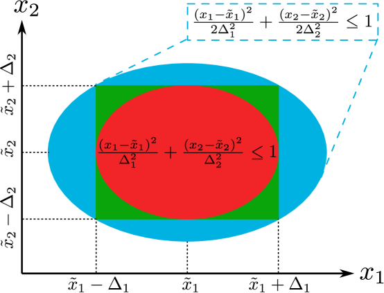
Figure 1: Ellipses constructed that either inscribe and circumscribe the original rectangular interval. We can construct ellipses from our square interval using the pictured equations. For a number of uncertain inputs $n>2$, the ellipse is generalized to a multivariate ellipsoid.

The choice for the ellipse to inscribe or circumscribe the rectangle depends principally on whether or not it is safe to exclude the corner regions of the rectangular parameter domain. If one is confident that the jointly extreme combinations of the input variables do not occur in the modeled system, as might be tenable if one assumes their uncertainties are independent, then the inscribed ellipse is safe, as it is a subset of the rectangular uncertainty domain. If one is not sure that the maxima and minima will not occur on the corners of the input uncertainty domain, the safe path is to select the circumscribed ellipse and ensure that the optimization domain is at least as large as that within the rectangle. One caveat, here, follows from areas within the circumscribed ellipsoid being outside of the $n$-dimensional rectangle. These regions of parameter space may not be physically realizable, which could potentially lead to an unrealistic optimization solution, for which the black box function may be difficult to evaluate.

The ellipsoid serves as a constraint on the model, and there are many possible circumscribing ellipsoids for a given rectangle. We chose to minimize the volume of the $n$-dimensional circumscribing ellipsoids for a given $n$-dimensional rectangle and performed the fit accordingly. Ultimately, the goal is to find the maximum and minimum of an objective function, which for the QRSM method is a quadratic function given by

$$f(x_{1},...,x_{n})=f_{0}+\sum_{i=1}^{n}f_{i}\cdot x_{i}\ +\sum_{i=1}^{n}\sum_{j=1}^{n}f_{i,j}\cdot x_{i}\cdot x_{j}$$ (3)

that approximates the output of the black box model over the domain of the input parameters. Equation (3) describes a multivariate quadratic model, and one can obtain the coefficients $f_{0}$, $f_{i}$, and $f_{i,j}$ by obtaining a fit to the output data using multivariate quadratic regression analysis. The output of the black-box model is then approximately bounded by the maximum and minimum of equation (3) over the ellipsoidal regions in the input parameter domain.

3 Case Study: the MESA Simulation Instrument

The instrument we treat as our black box code for this study is MESA (Modules for Experiments in Stellar Astrophysics) [7, 8, 9]. The MESA code is open source and is widely used in astrophysical research. It is an excellent example of a community code that is the culmination of years of development. As might be expected from incorporating multiple physical effects on multiple scales, the algorithms in MESA are complicated and defy the relatively easy analysis needed to analytically propagate incertitude in input parameters.

We applied the two advanced incertitude propagation techniques to the problem of evolving stars with MESA. Specifically, we performed suites of simulations evolving zero age main sequence (ZAMS) stars through their lives until they become C/O white dwarfs. The simulations were based on a setup available in the MESA test suite, 1M_pre_ms_to_wd, with models of 1 $M_{\odot}$ with a solar metallicity, $Z_{\odot}$ = 0.02, and the stars were evolved to a luminosity of 0.1$L_{\odot}$, the endpoint of stellar evolution.

Stellar winds are the mechanism of mass loss during the evolution of stars, but a first-principles understanding of these remains elusive. Instead, descriptions are parameterized by stellar properties such as luminosity, mass, and radius. MESA implements a number of prescriptions for mass loss during evolution on the red giant branch (RGB) and asymptotic giant branch (AGB) [10, 11, 12, 13]. For simplicity in this study, we chose models of the winds during these phases that do not assume a temperature dependence.

The two epistemically uncertain parameters for these winds are the Reimers and Blöckers scaling factors, $\eta^{\phantom{2}}_{R}$ and $\eta^{\phantom{2}}_{B}$, corresponding to RGB winds and AGB winds respectively. These parameters describe the RGB mass loss rate [11] and AGB mass loss rate [12], as

$$\dot{M}_{R}=4\cdot 10^{-13}\text{ }\eta^{\phantom{2}}_{R}\text{ }\frac{LR}{M}\text{ }[M_{\odot}\text{ yr}^{-1}]$$ (4)

and

$$\dot{M}_{B}=1.932\cdot 10^{-21}\text{ }\eta^{\phantom{2}}_{B}M^{-3.1}\cdot L^{3.7}R\text{ }[M_{\odot}\text{ yr}^{-1}]\;.$$ (5)

Here $L$, $M$, and $R$ are the luminosity, mass, and radius of the star in solar units. The scaling factors, $\eta^{\phantom{2}}_{R}$ and $\eta^{\phantom{2}}_{B}$, describe the strength of the winds and MESA expresses these through the controls Reimers_scaling_factor and Blocker_scaling_factor, respectively.

4 Results

In this section, we describe performing suites of simulations with MESA and applying the methods of uncertainty quantification. The results for each suite are a range of white dwarf masses presenting the bounds on the mass given the incertitude of our input.

We began our study with a regularly sampled uniform grid with $\eta^{\phantom{2}}_{B}$ sampled between 0.0 and 0.1, and $\eta^{\phantom{2}}_{R}$ was sampled between 0.4 and 0.9. These values were chosen following an earlier study of $1.0M_{\odot}$ ZAMS mass stars with similar evolution tracks in [14] and [15]. The results are shown in figure 2.

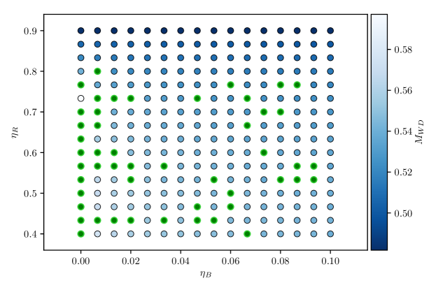
Figure 2: Initial regular grid of 256 $1.0M_{\odot}$ ZAMS models. The axes show $\eta^{\phantom{2}}_{R}$ vs. $\eta^{\phantom{2}}_{B}$, and the colormap indicated the final CO WD star masses. Models for which the simulations did not complete are highlighted in green.

Points at $\eta^{\phantom{2}}_{B}=0.0$ failed to complete for lower values of $\eta^{\phantom{2}}_{R}$, as seen in the figure. After this initial study, the domain was slightly adjusted so that $\eta^{\phantom{2}}_{B}$ was sampled regularly between 0.01 and 0.1 and $\eta^{\phantom{2}}_{R}$ was sampled regularly between 0.3 and 0.9. In addition to an initial exploration, this suite of regularly sampled simulations also served as a baseline with which to compare the CD and and QRSM methods. We note that any robust method for incertitude propagation must be able to accommodate the realistic situation that simulation codes are unable to carry out simulations for all values of input parameters for a variety of reasons. In this regard, MESA is a typical proxy for many other astrophysical simulation codes.

We next performed a suite of 200 simulations randomly sampled from a uniform distribution. In this case, results from simulations that did not complete are omitted. This suite better illustrated the parameter space, particularly the obvious nonlinearity. Figure 3 depicts the results of this suite of simulations.

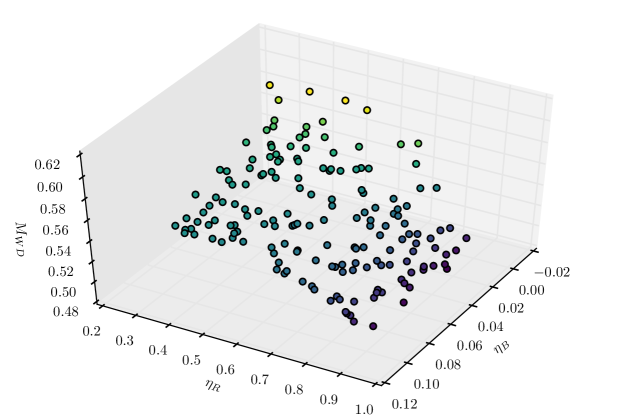
Figure 3: A suite of 200 models with values of $\eta^{\phantom{2}}_{R}$ and $\eta^{\phantom{2}}_{B}$ chosen at random from a uniform distribution between $\eta^{\phantom{2}}_{R}=[0.3,0.9]$ and $\eta^{\phantom{2}}_{B}=[0.01,0.1]$.

For this suite, the minimum sampled mass is 0.4902 $M_{\odot}$, and the maximum sampled mass is 0.5984 $M_{\odot}$.

The obvious nonlinearity observed in the first two suites of simulations indicated modification of the CD method would be required. As explained by [5], a way to deal with non-linearity is to subdivide the parameter space into linear sections and for each calculate a set of Cauchy-distributed inputs within the intervals. When bounds are found for each section, the maximum of the maxima and the minimum of the minima produce the bounds for the full space. Figure 4 illustrates the resultant tiles.

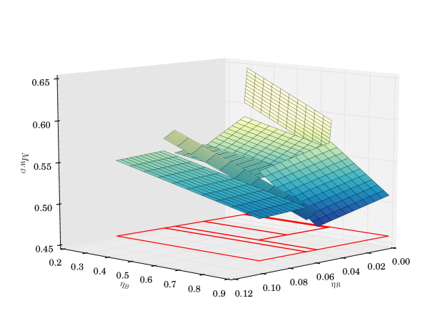
Figure 4: Parameter space broken up into 6 linear planes for application of the CD approach to uncertainty quantification. Linear tiles are determined via a region-growing algorithm that fits planes to samples of the parameter space subject to a constraint of the coefficient of determination for each plane fit.

For the suites of simulations that went into the CD study, we found an interval 0.5395 $\pm$ 0.0542 $M_{\odot}$ with a standard deviation of 0.0077 $M_{\odot}$, giving the range as [0.4776, 0.6014] [0.4699, 0.6091] [0.4622, 0.6168] $M_{\odot}$ with 68.3%, 99.5%, and 99.7% confidence, respectively.

The objective function found for our QRSM study is given by

$$\begin{aligned} M_{\rm WD}=f(\eta^{\phantom{2}}_{B},\eta^{\phantom{2}}_{R})=\;&\;0.5596-1.1323~{}\eta^{\phantom{2}}_{B}+0.1378~{}\eta^{\phantom{2}}_{R}\\ &+5.7688~{}\eta_{B}^{2}-0.2060~{}\eta_{R}^{2}\\ &+0.4646~{}\eta^{\phantom{2}}_{B}\cdot\eta^{\phantom{2}}_{R}\;,\end{aligned}$$ (6)

where the coefficients $f_{0}$, $f_{i}$, and $f_{i,j}$ in equation 3 have been replaced by the actual values obtained by fitting (see figure 5 below). For the purpose of obtaining the objective function, the sampling was done over the actual incertitude domain instead of on either the inner or outer ellipse. The computation of the output incertitude range based on the objective function is, however, found using the elliptical constraints. Figure 5 illustrates the quadratic regression fit.

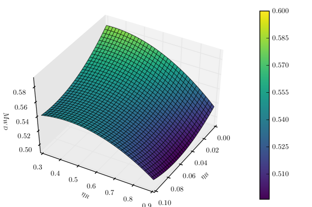
Figure 5: Surface plot of the multivariate quadratic regression fit. Note that the maximum and minimum are on the edges—there are no local extrema within the space.

For our QRSM study, we found ranges [0.4979,0.5606] $M_{\odot}$ and [0.4811,0.6119] $M_{\odot}$ for the inscribed and circumscribed ellipses, respectively.

5 Discussion and Conclusions

The purpose of this manuscript is to present the methodology for a study of incertitude propagation in black box simulation codes, and the results presented here, ranges of white dwarf masses, are not definitive. We presented this study as a look at work in progress and defer final calculated ranges to the complete work [4]. As may be seen in the results from the first uniform grid of points in the input parameter domain, many of the MESA simulations did not converge. While it is possible to produce more robust simulations with MESA by “tuning” the input to improve convergence, we specifically did not do this so as to keep our black box completely consistent for all simulations. The complete study will review the issue of convergence of the simulations. Our conclusion is that these methods, CD and QRSM, allow the formal propagation of the input incertitude into incertitude intervals of the simulation outputs in a straight forward and computationally tractable way.

In this case study, we utilized only two variables with incertitude. The full advantage of the advanced methods that we demonstrated, CD and QRSM, does not become apparent until applied to higher dimensional incertitude problems. One might be tempted to conclude that since the case study problem can be broken up into linear sub regions that one could easily evaluate the model at the extrema of the incertitude ranges. While this could be easily done for the two-dimensional case, in a situation with $n$ uncertain input parameters, this approach would require $2^{n}$ model evaluations to estimate the output uncertainty of the model. This is the so-called curse of dimensionality. In contrast, the advanced methods require far fewer model evaluations in order to estimate the model output uncertainty.

Another comparison we wish to make is between the CD and QRSM methods. The CD method has an advantage in that one has some knowledge of how many model sample points are needed in order to specify the desired confidence in the estimate of the model output uncertainty. In contrast, with the QRSM method there is no statistical knowledge of how many sample points are needed in order assess the precision with which the model output incertitude is known. The QRSM method, however, does posses two advantages over the CD method. First, the QRSM method makes no assumption of linearity and does not require subdividing the input parameter incertitude intervals into quasi-linear sub-intervals, thereby avoiding computationally costly model evaluations needed to evaluate the degree of linearity. Second, the QRSM method potentially can require far fewer model evaluations in that as few as $n(n-1)/2+2n+1$ are needed to determine the coefficients of the ellipsoid given in equation 3. In a situation where $n$ is large, this property could result in a significant advantage realized through the use of the QRSM method. One can only gain confidence in the estimates of the model output uncertainty, however, by carrying out a convergence test where the number of sample points is increased. The minimum number of points yields an exact output uncertainty only in the case of a perfectly quadratic model.

Finally, we wish to point out a limitation on the interpretation of the output model response. This response cannot be physically interpreted as a probability distribution because the distribution of input parameters is unknown by definition of incertitude. All that can be determined in the case of input incertitudes is a model output uncertainty. Were the distributions of the input uncertainties known, the output response could have an interpretation as a probability distribution. The methods described here, however, are not suitable to address this problem. Research into uncertainty quantification for the problem of known distributions of input uncertainties, however, is underway.

The source code for the tools applied to this study, Star Simulation Techniques for Research in Uncertainty Quantification, is freely available at https://github.com/StarSTRUQ. The site includes the software for generating the Cauchy deviates samples, performing the QRSM analysis, and the tiling, which subdivides a sampled domain into planar tiles constrained by the planar fit.

This work was supported in part by the US Department of Energy under grant DE-FG02-87ER40317 and by the US National Science Foundation under grant AST-1211563. The research described here originated with co-author Melissa Hoffman’s thesis at Stony Brook University. The simulations performed for this study were performed with the MESA stellar evolution code and the authors thank its developers and community for making this resource available. The authors would like to thank Stony Brook Research Computing and Cyberinfrastructure, and the Institute for Advanced Computational Science at Stony Brook University for access to the high-performance LIred and SeaWulf computing systems, the latter of which was made possible by a $1.4M National Science Foundation grant (#1531492). The authors also thank Tracy M. Calder for previewing the manuscript. This research has made use of NASA’s Astrophysics Data System Bibliographic Services.

References

References

- [1] Roache P 1998 Verification and Validation in Computational Science and Engineering (Hermosa) ISBN 9780913478080 URL https://books.google.com/books?id=ENRlQgAACAAJ
- [2] Oberkampf W and Roy C 2010 Verification and Validation in Scientific Computing (Cambridge University Press) ISBN 9781139491761 URL https://books.google.com/books?id=7d26zLEJ1FUC
- [3] AIAA 1998 AIAA Guide for the Verification and Validation of Computational Fluid Dynamics Simulations AIAA G: American Institute of Aeronautics and Astronautics (American Institute of Aeronautics and Astronautics) ISBN 9781563472855 URL https://books.google.com/books?id=OUAHAAAACAAJ
- [4] Hoffman M M, Willcox D E, Katz M P, Ferson S and Swesty F D 2017 in preparation, to be submitted to ApJ
- [5] Kreinovich V and Ferson S 2004 Reliability Engineering and System Safety 85 267–279 ISSN 0951-8320
- [6] Kreinovich V, Hajagos J G, Tucker W T, Ginzburg L R and Ferson S 2008 Propagating uncertainty through a quadratic response surface model Tech. Rep. SAND2008-5983 Sandia National Laboratory
- [7] Paxton B, Bildsten L, Dotter A, Herwig F, Lesaffre P and Timmes F 2011 ApJS 192 3 (Preprint 1009.1622)
- [8] Paxton B, Cantiello M, Arras P, Bildsten L, Brown E F, Dotter A, Mankovich C, Montgomery M H, Stello D, Timmes F X and Townsend R 2013 ApJS 208 4 (Preprint 1301.0319)
- [9] Paxton B, Marchant P, Schwab J, Bauer E B, Bildsten L, Cantiello M, Dessart L, Farmer R, Hu H, Langer N, Townsend R H D, Townsley D M and Timmes F X 2015 ApJS 220 15 (Preprint 1506.03146)
- [10] Reimers D 1975 Memoires of the Societe Royale des Sciences de Liege 8 369–382
- [11] Reimers D 1975 Circumstellar envelopes and mass loss of red giant stars pp 229–256
- [12] Blöcker T 1995 A&A 297 727
- [13] de Jager C, Nieuwenhuijzen H and van der Hucht K A 1988 A&AS 72 259–289
- [14] Karakas A I and Lugaro M 2016 ApJ 825 26 (Preprint 1604.02178)
- [15] Pignatari M, Herwig F, Hirschi R, Bennett M, Rockefeller G, Fryer C, Timmes F X, Ritter C, Heger A, Jones S, Battino U, Dotter A, Trappitsch R, Diehl S, Frischknecht U, Hungerford A, Magkotsios G, Travaglio C and Young P 2016 ApJS 225 24 (Preprint 1307.6961)