How Many Machines Can We Use in Parallel Computing for Kernel Ridge Regression?

Abstract

This paper aims to solve a basic problem in distributed statistical inference: how many machines can we use in parallel computing? In kernel ridge regression, we address this question in two important settings: nonparametric estimation and hypothesis testing. Specifically, we find a range for the number of machines under which optimal estimation/testing is achievable. The employed empirical processes method provides a unified framework, that allows us to handle various regression problems (such as thin-plate splines and nonparametric additive regression) under different settings (such as univariate, multivariate and diverging-dimensional designs). It is worth noting that the upper bounds of the number of machines are proven to be un-improvable (upto a logarithmic factor) in two important cases: smoothing spline regression and Gaussian RKHS regression. Our theoretical findings are backed by thorough numerical studies.

Key Words: Computational limit, divide and conquer, kernel ridge regression, minimax optimality, nonparametric testing.

1 Introduction

In the parallel computing environment, a common practice is to distribute a massive dataset to multiple processors, and then aggregate local results obtained from separate machines into global counterparts. This Divide-and-Conquer (D&C) strategy often requires a growing number of machines to deal with an increasingly large dataset. An important question to statisticians is ”how many machines can we use in parallel computing to guarantee statistical optimality?” The present work aims to explore this basic yet fundamentally important question in a classical nonparametric regression setup, i.e., kernel ridge regression (KRR). This can be done by carefully analyzing statistical versus computational trade-off in the D&C framework, where the number of deployed machines is treated as a simple proxy for computing cost.

Recently, researchers have made impressive progress about KRR in the modern D&C framework with different conquer strategies; examples include median-of-means estimator proposed by [11], Bayesian aggregation considered by [15, 22, 18, 20], and simple averaging considered by [29] and [16]. Upper bounds for the number of machines $s$ have been studied in such strategies to guarantee good property. For instance, [29] showed that, when $s$ processors are employed with $s$ in a suitable range, D$\&$C method still preserves minimax optimal estimation. In smoothing spline regression (a special case of KRR), [16] derived critical, i.e., un-improvable, upper bounds for $s$ to achieve either optimal estimation or optimal testing, but their results are only valid in univariate fixed design. The critical bound for estimation obtained by [16] significantly improves the one given in [29]. Nonetheless, it remains unknown if results obtained in [16] continues to hold in a more general KRR framework where the design is either multivariate or random. On the other hand, there is a lack of literature dealing with nonparametric testing in general KRR. To the best of our knowledge, [16] is the only reference but in the special smoothing spline regression with univariate fixed designs.

In this paper, we consider KRR in the D$\&$C regime in a general setup: design is random and multivariate. As our technical contribution, we characterize the upper bounds of $s$ for achieving optimal estimation and testing based on quantifying an empirical process (EP), such that a sharper concentration bound of the EP leads to a tighter upper bound of $s$. Our EP approaches can handle various function spaces including Sobolev space, Gaussian RKHS, or spaces of special structures such as additive functions, in a unified manner. As an illustration example, in the particular smoothing spline regression, we introduce the Green function for equivalent kernels to the EP bound and achieve a polynomial order improvement of $s$ compared with [29]. It is worthy noting that our upper bound is almost identical as [16] (upto a logarithmic factor) for optimal estimation, which is proven to be un-improvable.

The second main contribution of this paper is to propose a Wald type test statistic for nonparametric testing in D&C regime. Asymptotic null distribution and power behaviors of the proposed test statistic are carefully analyzed. One important finding is that the upper bounds of $s$ for optimal testing are dramatically different from estimation, indicating the essentially different natures of the two problems. Our testing results are derived in a general framework that cover the aforementioned important function spaces. As an important byproduct, we derive a minimax rate of testing for nonparametric additive models with diverging number of components which is new in literature. Such rate is crucial in deriving the upper bound for $s$ for optimal testing, and is of independent interest.

2 Background and Distributed Kernel Ridge Regression

We begin by introducing some background on reproducing kernel Hilbert space (RKHS), and our nonparametric testing formulation under the distributed kernel ridge regression.

2.1 Nonparametric regression in reproducing kernel Hilbert spaces

Suppose that data $\{(Y_{i},X_{i}):i=1,\ldots,N\}$ are iid generated from the following regression model

$$Y_{i}=f(X_{i})+\epsilon_{i},\,\,i=1,\ldots,N,$$ (2.1)

where $\epsilon_{i}$ are random errors with $E\{\epsilon_{i}\}=0$, $E\{\epsilon_{i}^{2}|X_{i})=\sigma^{2}(X_{i})>0$, the covariates $X_{i}\in\mathcal{X}\subseteq\mathbb{R}^{d}$ follows a distribution $\pi(x)$, and $Y_{i}\in\mathbb{R}$ is a real-valued response. Here, $d\geq 1$ is either fixed or diverging with $N$, and $f$ is unknown.

Throughout we assume that $f\in\mathcal{H}$, where $\mathcal{H}\subset L_{\pi}^{2}(\mathcal{X})$ is a reproducing kernel Hilbert space (RKHS) associated with an inner product $\langle\cdot,\cdot\rangle_{\mathcal{H}}$ and a reproducing kernel function $R(\cdot,\cdot):\mathcal{X}\times\mathcal{X}\to\mathbb{R}$. By Mercer’s Theorem, $R$ has the following spectral expansion ([21]):

$$R(x,x^{\prime})=\sum_{i=1}^{\infty}\mu_{i}\varphi_{i}(x)\varphi_{i}(x^{\prime}),\,\,\,\,x,x^{\prime}\in\mathcal{X},$$

where $\mu_{1}\geq\mu_{2}\geq\cdots\geq 0$ is a sequence of eigenvalues and $\{\varphi_{i}\}_{i=1}^{\infty}$ form a basis in $L_{\pi}^{2}(\mathcal{X})$. Moreover, for any $i,j\in\mathbb{N}$,

$$\langle\varphi_{i},\varphi_{j}\rangle_{L_{\pi}^{2}(\mathcal{X})}=\delta_{ij}\quad\quad\text{and}\quad\quad\langle\varphi_{i},\varphi_{j}\rangle_{\mathcal{H}}=\delta_{ij}/\mu_{i},$$

where $\delta_{ij}$ is Kronecker’s $\delta$.

We introduce a norm $\|\cdot\|$ in $\mathcal{H}$ by combining the $L_{2}$ norm and $\|\cdot\|_{\mathcal{H}}$ norm to facilitate our statistical inference theory. For $f,g\in\mathcal{H}$, define

$$\langle f,g\rangle=V(f,g)+\lambda\langle f,g\rangle_{\mathcal{H}},$$ (2.2)

where $V(f,g)=E\{f(X)g(X)\}$ and $\lambda>0$ is the penalization parameter. Clearly, $\langle\cdot,\cdot\rangle$ defines an inner product on $\mathcal{H}$. It is easy to prove that $(\mathcal{H},\langle\cdot,\cdot\rangle)$ is also a RKHS with reproducing kernel function $K(\cdot,\cdot)$ satisfying the following so-called reproducing property:

$$\langle f,K_{x}(\cdot)\rangle=f(x),\;\;\text{for all }f\in\mathcal{H},$$

where $K_{x}(\cdot)=K(x,\cdot)$ for $x\in\mathcal{X}$.

For any $f\in\mathcal{H}$, we can express the function in terms of the Fourier expansion as $f=\sum_{\nu\geq 1}V(f,\varphi_{\nu})\varphi_{\nu}$. Therefore,

$$\langle f,\varphi_{\nu}\rangle=\sum_{i\geq 1}V(f,\varphi_{i})\langle\varphi_{i},\varphi_{\nu}\rangle=V(f,\varphi_{\nu})(1+\lambda/\mu_{\nu}).$$ (2.3)

Replacing $f$ with $K_{x}$ in (2.3), we have $V(K_{x},\varphi_{\nu})=\frac{\langle K_{x},\varphi_{\nu}\rangle}{1+\lambda/\mu_{\nu}}=\frac{\varphi_{\nu}(x)}{1+\lambda/\mu_{\nu}}$. Then for any $x,y\in\mathcal{X}$, $K(x,y)$ has an explicit eigen-expansion expressed as

$$K(x,y)=\sum_{\nu\geq 1}V(K_{x},\varphi_{\nu})\varphi_{\nu}(y)=\sum_{\nu\geq 1}\frac{\varphi_{\nu}(x)\varphi_{\nu}(y)}{1+\lambda/\mu_{\nu}}.$$

2.2 Distributed kernel ridge regression

For estimating $f$, we consider the kernel ridge regression (KRR) in a divide-and-conquer (D$\&$C) regime. First, randomly divide the $N$ samples into $s$ subsamples. Let $I_{j}$ denote the set of indices of the observations from subsample $j$ for $j=1,\ldots,s$. For simplicity, suppose $|I_{j}|=n$, i.e., all subsamples are of equal sizes. Hence, the total sample size is $N=ns$. Then, we estimate $f$ based on subsample $j$ through the following KRR method:

$$\widehat{f}_{j}=\mathop{\mathrm{argmin}}_{f\in\mathcal{H}}\ell_{j,\lambda}(f)\equiv\mathop{\mathrm{argmin}}_{f\in\mathcal{H}}\frac{1}{2n}\sum_{i\in I_{j}}(Y_{i}-f(X_{i}))^{2}+\frac{\lambda}{2}\|f\|_{\mathcal{H}}^{2},\,\,\,\,j=1,\ldots,s,$$

where $\lambda>0$ is the penalization parameter. The D$\&$C estimator of $f$ is defined as the average of $\widehat{f}_{j}$’s, that is, $\bar{f}=\sum_{j=1}^{s}\widehat{f}_{j}/s$.

Based on $\bar{f}$, we further propose a Wald-type statistic $T_{N,\lambda}:=\|\bar{f}\|^{2}$ for testing the hypothesis

$$H_{0}:f=0 H_{1}:f\in\mathcal{H}\backslash\{0\}$$, vs. . (2.4)

In general, testing $f=f_{0}$ (for a known $f_{0}$) is equivalent to testing $f_{\ast}\equiv f-f_{0}=0$. So, (2.4) has no loss of generality.

3 Main results

In this section, we derive some general results relating to $\bar{f}$ and $T_{N,\lambda}$. Let us first introduce some regularity assumptions.

3.1 Assumptions

The following Assumptions A1 and A2 require that the design density is bounded and the error $\epsilon$ has finite fourth moment, which are commonly used in literature, see [3].

Assumption A1.

There exists a constant $c_{\pi}>0$ such that for all $x\in\mathcal{X}$, $0\leq\pi(x),\sigma^{2}(x)\leq c_{\pi}$.

Assumption A2.

There exists a positive constant $\tau$ such that $E\{\epsilon^{4}|X\}<\tau$ almost surely.

Define $\|f\|_{\sup}=\sup_{x\in\mathcal{X}}|f(x)|$ as the supremum norm of $f$. We further assume that $\{\varphi_{\nu}\}_{\nu=1}^{\infty}$ are uniformly bounded on $\mathcal{X}$, and $\{\mu_{\nu}\}_{\nu=1}^{\infty}$ satisfy certain tail sum property.

Assumption A3.

$c_{\varphi}:=\sup_{j\geq 1}\|\varphi_{j}\|_{\sup}<\infty$ and $\sup_{k\geq 1}\frac{\sum_{\nu=k+1}^{\infty}\mu_{i}}{k\mu_{k}}<\infty$.

The uniform boundedness condition of eigen-functions holds for various kernels, example includes univariate periodic kernel, 2-dimensional Gaussian kernel, multivariate additive kernel; see [7], [10] and reference therein. The tail sum property can also be verified in various RKHS, and is deferred to the Appendix.

Define $h^{-1}:=\sum_{\nu\geq 1}\frac{1}{1+\lambda/\mu_{\nu}}$ as effective dimension. It has been widely studied in reference [1], [9], [28] etc. There is an explicit relationship between $h$ and $\lambda$ as illustrated in various concrete examples in Section 3.4. Another quantity of interest is the series $\sum_{\nu\geq 1}(1+\lambda/\mu_{\nu})^{-2}$, which represents the variance term defined in Theorem 3.5. In the following Proposition 3.1, we show that such variance term has the same order of $h^{-1}$.

Proposition 3.1.

Suppose Assumption A3 holds. For any $\lambda>0$, $\sum_{\nu\geq 1}(1+\lambda/\mu_{\nu})^{-2}\asymp h^{-1}$.

Define $Pf=E_{X}\{f(X)\}$, $P_{j}f=n^{-1}\sum_{i\in I_{j}}f(X_{i})$ and

$$\xi_{j}=\sup_{\begin{subarray}{c}f,g\in\mathcal{H}\\ \|f\|=\|g\|=1\end{subarray}}|P_{j}fg-Pfg|,\,\,1\leq j\leq s.$$

Here, $\xi_{j}$ is the supremum of the empirical processes based on subsample $j$. The quantity $\max_{1\leq j\leq s}\xi_{j}$ plays a vital role in determining the critical upper bound of $s$ to guarantee statistical optimality. As shown in our main theorems, a sharper bound of $\xi_{j}$ directly leads to an improved upper bound of $s$. Assumption A4 provides a concentration bound for $\xi_{j}$, and says that $\xi_{j}$ are uniformly bounded by $\sqrt{\frac{\log^{b}{N}}{nh^{a}}}$, $a,b$ are constants that are specified in various kernels. Verification of Assumption A4 is deferred to Section 3.4 in concrete settings based on empirical processes methods, where the values of $a,b$ will be explicitly specified.

Assumption A4.

There exist nonnegative constants $a,b$ such that

$$\max_{1\leq j\leq s}\xi_{j}=O_{P}\left(\sqrt{\frac{\log^{b}{N}}{nh^{a}}}\right).$$

3.2 Minimax optimal estimation

In this section, we derive a general error bound for $\bar{f}$. Let $\textbf{X}_{j}=\{X_{i}:i\in I_{j}\}$ and $\textbf{X}=\{\textbf{X}_{1},\ldots,\textbf{X}_{s}\}$. Suppose that (2.1) holds under $f=f_{0}$. For convenience, let $\mathcal{P}_{\lambda}$ be a self-adjoint operator from $\mathcal{H}$ to itself such that $\langle\mathcal{P}_{\lambda}f,g\rangle=\lambda\langle f,g\rangle_{\mathcal{H}}$ for all $f,g\in\mathcal{H}$. The existence of $\mathcal{P}_{\lambda}$ follows by [14, Proposition 2.1]. We first obtain a uniform error bound for $\widehat{f}_{j}$’s in the following Lemma 3.2.

Lemma 3.2.

Suppose Assumptions A1,A3,A4 are satisfied and $\log^{b}{N}=o(nh^{a})$ with $a,b$ given in Assumption A4. Then with probability approaching one, for any $1\leq j\leq s$,

$$E\{\|\widehat{f}_{j}-E\{\widehat{f}_{j}|\textbf{X}_{j}\}-\frac{1}{n}\sum_{i\in I_{j}}\epsilon_{i}K_{X_{i}}\|^{2}|\textbf{X}_{j}\} \leq \frac{4c_{\pi}c_{\varphi}^{2}\xi_{j}^{2}}{nh},$$ (3.1)

$$\|E\{\widehat{f}_{j}|\textbf{X}_{j}\}-f_{0}+\mathcal{P}_{\lambda}f_{0}\| \leq 2\xi_{j}\lambda^{1/2}\|f_{0}\|_{\mathcal{H}}$$ (3.2)

(3.1) quantifies the deviation from $\widehat{f}_{j}$ to its conditional mean through a higher order remainder term, and (3.2) quantifies the bias of $\widehat{f}_{j}$. Lemma 3.2 immediately leads to the following result on $\bar{f}$. Specifically, (3.1) and (3.2) lead to (3.3), which, together with the rates of $\sum_{i=1}^{N}\epsilon_{i}K_{X_{i}}$ and $\mathcal{P}_{\lambda}f_{0}$ in Lemma A.1, leads to (3.4).

Theorem 3.3.

If the conditions in Lemma 3.2 hold, then with probability approaching one,

$$E\{\|\bar{f}-\frac{1}{N}\sum_{i=1}^{N}\epsilon_{i}K_{X_{i}}-f_{0}+\mathcal{P}_{\lambda}f_{0}\|^{2}|\textbf{X}\} \leq 4\left(\frac{c_{\pi}c_{\varphi}^{2}}{Nh}+\lambda\|f_{0}\|^{2}_{\mathcal{H}}\right)\max_{1\leq j\leq s}\xi_{j}^{2},$$ (3.3)

$$E\{\|\bar{f}-f_{0}\|^{2}|\textbf{X}\} \leq \frac{4c_{\pi}c_{\varphi}^{2}}{Nh}+8\lambda\|f_{0}\|^{2}_{\mathcal{H}}.$$ (3.4)

Theorem 3.3 is a general result that holds for many commonly used kernels. Note that $n=N/s$, the condition $\log^{b}N=o(nh^{a})$ directly implies that as long as $s$ is dominated by $Nh^{a}/\log^{b}N$, the conditional mean squared errors can be upper bounded by the variance term $(Nh)^{-1}$ and the squared bias term $\lambda\|f_{0}\|^{2}_{\mathcal{H}}$. Then the minimax optimal estimation can be obtained through the particular $\lambda$ that satisfies such bias-variance trade-off; see [1], [25]. Section 3.4 further illustrates concrete and interpretable guarantees on the conditional mean squared errors to particular kernels.

It is worthy to note that, through the condition of Lemma 3.2 and Theorem 3.3, we build a direct connection between the upper bound of $s$ and the uniform bound of the empirical process $\xi_{j}$. That is, a tighter upper bound of $s$ can be achieved by a sharper concentration bound of $\max_{1\leq j\leq s}\xi_{j}$, which is guaranteed by the empirical process methods in this work. For instance, in Section 3.4.1 the smoothing spline regression, we introduce the Green function for equivalent kernels in [3] to provide a sharp concentration bound of $\xi_{j}$ with $a=b=1$. Consequently, we achieve an upper bound for $s$ almost identical to the critical one obtained by [16] (upto a logarithmic factor), and improve the one obtained by [29] in polynomial order.

3.3 Minimax optimal testing

In this section, we derive the asymptotic distribution of $T_{N,\lambda}:=\|\bar{f}\|^{2}$ and further investigate its power behavior. For simplicity, assume that $\sigma^{2}(x)\equiv\sigma^{2}$ is known. Otherwise, we can replace $\sigma^{2}$ by its consistent estimator to fulfill our procedure. We will show that the distributed test statistic $T_{N,\lambda}$ can achieve minimax rate of testing (MRT), provided that the number of divisions $s$ belongs to a suitable range. Here, MRT is defined as the minimal distance between the null and the alternative hypotheses such that valid testing is possible. The range of $s$ is determined based on the criteria that the proposed test statistic can asymptotically achieve correct size and high power.

Before proving consistency of the test statistics $T_{N,\lambda}$, i.e., Theorem 3.5, let us state a technical lemma. Define $W(N)=\sum_{1\leq i<k\leq N}W_{ik}$ with $W_{ik}=2\epsilon_{i}\epsilon_{k}K(X_{i},X_{k})$, and let $\sigma^{2}(N)=\textrm{Var}(W(N))$. Define the empirical kernel matrix $\textbf{K}=[K(X_{i},X_{j})]_{i,j=1}^{N}$ and $\bm{\epsilon}=(\epsilon_{1},\ldots,\epsilon_{N})^{T}$.

Lemma 3.4.

Suppose Assumptions A1,A2, A3, A4 are all satisfied, and $N\to\infty$, $h=o(1)$, $Nh^{2}\to\infty$. Then it holds that

$$\bm{\epsilon}^{\prime}\textbf{K}\bm{\epsilon}=\sigma^{2}Nh^{-1}+W(N)+O_{P}(\sqrt{Nh^{-2}}).$$ (3.5)

Furthermore, as $N\to\infty$, $\frac{W(N)}{\sigma(N)}\overset{d}{\longrightarrow}N(0,1)$, where $\sigma^{2}(N)=2\sigma^{4}N(N-1)\sum_{\nu\geq 1}\frac{1}{(1+\lambda/\mu_{\nu})^{2}}\asymp N^{2}h^{-1}$.

The following theorem shows that $T_{N,\lambda}$ is asymptotically normal under $H_{0}$. The key condition to obtain such a result is $\log^{b}N=o(nh^{a+1})$, where $a,b$ are determined through the uniform bound of $\xi_{j}$ in Assumption A4. This condition in turn leads to upper bounds for $s$ to achieve MRT; see Section 3.4 for detailed illustrations.

Theorem 3.5.

Suppose Assumptions A1 to A4 are all satisfied, and as $N\to\infty$, $h=o(1)$, $Nh^{2}\to\infty$, and $\log^{b}N=o(nh^{a+1})$. Then, as $N\to\infty$,

$$\frac{N^{2}}{\sigma(N)}\left(T_{N,\lambda}-\frac{\sigma^{2}}{Nh}\right)\overset{d}{\longrightarrow}N(0,1).$$

By Theorem 3.5, we can define an asymptotic testing rule with $(1-\alpha)$ significance level as follows:

$$\psi_{N,\lambda}=I\left(|T_{N,\lambda}-\sigma^{2}/(Nh)|\geq z_{1-\alpha/2}\sigma(N)/N^{2}\right),$$

where $z_{1-\alpha/2}$ is the $(1-\alpha/2)\times 100$ percentile of standard normal distribution.

For any $f\in\mathcal{H}$, define

$$b_{N,\lambda} =(\lambda^{1/2}\|f\|_{\mathcal{H}}+(Nh)^{-1/2})\sqrt{\frac{\log^{b}{N}}{nh^{a}}},\,\,\,\,\textrm{and}$$

$$d_{N,\lambda} =\lambda^{1/2}\|f\|_{\mathcal{H}}+(Nh^{1/2})^{-1/2}+N^{-1/2}+b_{N,\lambda}^{1/2}(Nh)^{-1/4}+b_{N,\lambda}.$$

$d_{N,\lambda}$ is used to measure the distance between the null and the alternative hypotheses. The following Theorem 3.6 shows that, if the alternative signal $f$ is separated from zero by an order $d_{N,\lambda}$, then the proposed test statistic asymptotically achieves high power. To achieve optimal testing, it is sufficient to minimize $d_{N,\lambda}$. As long as $s$ is dominated by $(Nh^{a+1}/\log^{b}N)$, $d_{N,\lambda}$ can be simplified as

$$d_{N,\lambda}\asymp\quad\underbrace{\lambda^{1/2}\|f\|_{\mathcal{H}}}_{\textrm{Bias of }\bar{f}}\quad+\underbrace{(Nh^{1/2})^{-1/2}}_{\textrm{Standard deviation of }T_{N,\lambda}}$$ (3.6)

Then, MRT can be achieved by selecting $\lambda$ to balance the tradeoff between the bias of $\bar{f}$ and the standard derivation of $T_{N,\lambda}$; see [6], [23]. It is worth noting that, such a tradeoff in (3.6) for testing is different from the bias-variance tradeoff in (3.3) for estimation, thus leading to different optimal testing rate.

Theorem 3.6.

If the conditions in Theorem 3.5 hold, then for any $\varepsilon>0$, there exist $C_{\varepsilon}$ and $N_{\varepsilon}$ s.t.

$$\inf_{\begin{subarray}{c}\|f\|\geq C_{\varepsilon}d_{N,\lambda}\end{subarray}}P_{f}(\psi_{N,\lambda}=1)\geq 1-\varepsilon,\,\,\,\,\textrm{for any $N\geq N_{\varepsilon}$.}$$

Section 3.4 will develop upper bounds for $s$ in various concrete examples based on the above general theorems. Our results will indicate that the ranges for $s$ to achieve MRT are dramatically different from ones to achieve optimal estimation.

3.4 Examples

In this section, we derive upper bounds for $s$ in four featured examples to achieve optimal estimation/testing, based on the general results obtained in Sections 3.2 and 3.3. Our examples cover the settings of univariate, multivariate and diverging-dimensional designs.

3.4.1 Example 1: Smoothing spline regression

Suppose $\mathcal{H}=\{f\in S^{m}(\mathbb{I}):\|f\|_{\mathcal{H}}\leq C\}$ for a constant $C>0$, where $S^{m}(\mathbb{I})$ is the $m$th order Sobolev space on $\mathbb{I}\equiv[0,1]$, i.e.,

$$S^{m}(\mathbb{I})=\big{\{}f\in L^{2}(\mathbb{I})|\, f^{(j)}\mbox{ are abs. cont. for}\;j=0,1,\ldots,m-1,\;$$

$$\mbox{and}\;\int_{\mathbb{I}}|f^{(m)}(x)|^{2}dx<\infty\big{\}},$$

and $\|f\|_{\mathcal{H}}=\int_{\mathbb{I}}|f^{(m)}(x)|^{2}dx$. Then model (2.1) becomes the usual smoothing spline regression. In addition to Assumption A1, we assume that

$$c_{\pi}^{-1}\leq\pi(x)\leq c_{\pi},\,\,\textrm{for any $x\in\mathbb{I}$.}$$ (3.7)

We call the design satisfying (3.7) as quasi-uniform, a common assumption on many statistical problems; see [3]. Quasi-uniform assumption excludes cases where design density is (nearly) zero at certain data points, which may cause estimation inaccuracy at those points.

It is known that when $m>1/2$, $S^{m}(\mathbb{I})$ is a RKHS under the inner product $\langle\cdot,\cdot\rangle$; see [14], [4]. Meanwhile, Assumption A3 holds with kernel eigenvalues $\mu_{\nu}\asymp\nu^{-2m}$, $\nu\geq 1$. Hence, Proposition 3.1 holds with $h\asymp\lambda^{1/(2m)}$. We next provide a sharp concentration inequality to bound $\xi_{j}$.

Proposition 3.7.

Under (3.7), there exist universal positive constants $c_{1},c_{2},c_{3}$ such that for any $1\leq j\leq s$,

$$P\left(\xi_{j}\geq t\right)\leq 2n\exp\left(-\frac{nht^{2}}{c_{1}+c_{2}t}\right),\,\,\textrm{for all $t\geq c_{3}(nh)^{-1}$.}$$

The proof of Proposition 3.7 is based on the novel technical tool that we introduce into D$\&$C framework: the Green function for equivalent kernels; see [3, Corollary 5.41]. An immediate consequence of Proposition 3.7 is that Assumption A4 holds with $a=b=1$. Then based on Theorem 3.3 and Theorem 3.6, we have the following results.

Corollary 3.8.

Suppose that $\mathcal{H}=S^{m}(\mathbb{I})$, (3.7), Assumptions A1 and A2 hold.

1. If $m>1/2$, $s=o(N^{2m/(2m+1)}/\log{N})$ and $\lambda\asymp N^{-2m/(2m+1)}$, then $\|\bar{f}-f_{0}\|=O_{P}(N^{-m/(2m+1)})$.

2. If $m>3/4$, $s=o(N^{(4m-3)/(4m+1)}/\log{N})$ and $\lambda\asymp N^{-4m/(4m+1)}$, then the Wald-type test achieves minimax rate of testing $N^{-2m/(4m+1)}$.

It is known that the estimation rate $N^{-m/(2m+1)}$ is minimax-optimal; see [19]. Furthermore, the testing rate $N^{-2m/(4m+1)}$ is also minimax optimal, in the sense of [6]. It is worth noting that the upper bound for $s=o(N^{2m/(2m+1)}/\log{N})$ matches (upto a logarithmic factor) the critical one by [16] in evenly spaced design, which is substantially larger than the one obtained by [29], i.e., $s=o(N^{(2m-1)/(2m+1)}/\log{N})$ for bounded eigenfunctions; see Table 1 for the comparison.

	Zhang et al [29]	Shang et al [16]	Our approach
smoothing spline regression	$s\lesssim N^{\frac{2m-1}{2m+1}}/\log N$ sharpness of $s$ ✗	$s\lesssim N^{\frac{2m}{2m+1}}$ sharpness of $s$ ✓	$s=o(N^{\frac{2m}{2m+1}}/\log N)$ sharpness of $s$ ✓

Table 1: Comparison of upper bounds of $s$ to achieve minimax optimal estimation.

3.4.2 Example 2: Nonparametric additive regression

Consider the function space

$$\mathcal{H}=\{f(x_{1},\ldots,x_{d})=\sum_{k=1}^{d}f_{k}(x_{k}):\,f_{k}\in S^{m}(\mathbb{I}),\;\|f_{k}\|_{\mathcal{H}}\leq C\;\text{for}\;k=1,\ldots,d\},$$

where $C>0$ is a constant. That is, any $f\in\mathcal{H}$ has an additive decomposition of $f_{k}$’s. Here, $d$ is either fixed or slowly diverging. Such additive model has been well studied in many literatures; see [19], [8], [13], [27] among others. For $x=(x_{1},\cdots,x_{d})\in\mathcal{X}$, suppose $x_{i},x_{j}$ are independent for $i\neq j\in\{1,\cdots,d\}$ and each $x_{i}$ satisfies (3.7). For identifiability, assume $E\{f_{k}(x_{k})\}=0$ for all $1\leq k\leq d$. For $f=\sum_{k=1}^{d}f_{k}$ and $g=\sum_{k=1}^{d}g_{k}$, define

$$\langle f,g\rangle_{\mathcal{H}} =\sum_{k=1}^{d}\langle f_{k},g_{k}\rangle_{\mathcal{H}}=\sum_{k=1}^{d}\int_{\mathbb{I}}f_{k}^{(m)}(x)g_{k}^{(m)}(x)dx,\quad\text{and}$$

$$V(f,g) =\sum_{k=1}^{d}V_{k}(f_{k},g_{k})\equiv\sum_{k=1}^{d}E\{f_{k}(X_{k})g_{k}(X_{k})\}.$$

It is easy to verify that $\mathcal{H}$ is an RKHS under $\langle\cdot,\cdot\rangle$ defined in (2.2). Lemma 3.9 below summarizes the properties for the $\mathcal{H}$ with $d$ additive components.

Lemma 3.9.

1. There exist eigenfunctions $\varphi_{\nu}$ and eigenvalues $\mu_{\nu}$ that satisfying Assumption A3.

2. It holds that $\sum_{\nu\geq 1}(1+\lambda/\mu_{\nu})^{-1}:=h^{-1}\asymp d\lambda^{-1/(2m)}$, and $\sum_{\nu\geq 1}(1+\lambda/\mu_{\nu})^{-2}\asymp h^{-1}$ accordingly.

3. For $f\in\mathcal{H}$, $\|\mathcal{P}_{\lambda}f\|^{2}\leq cd\lambda$, where $c$ is a bounded constant.

4. Assumption A4 holds with $a=b=1$.

Lemma 3.9 (4) establishes a concentration inequality of $\xi_{j}$ for the additive model, such that $\max_{1\leq j\leq s}=O_{P}(\sqrt{\frac{\log N}{nh}})$. The proof is based on the extension of the Green function techniques ([3]) to diverging dimensional setting; see Lemma A.2 in Appendix.

Combining Lemma 3.9, Theorems 3.3, 3.5 and 3.6, we have the following result.

Corollary 3.10.

1. Suppose Assumptions A1, A2 hold. If $m>1/2$, $d=o(N^{\frac{2m}{2m+1}}/\log N)$, $s=o(d^{-1}N^{\frac{2m}{2m+1}}/\log N)$, $\lambda\asymp N^{-\frac{2m}{2m+1}}$, then $\|\bar{f}-f_{0}\|=O_{P}(d^{1/2}N^{-\frac{m}{2m+1}})$.

2. Suppose Assumptions A1, A2 hold. If $m>3/4$, $d=o(N^{\frac{4m-3}{4(2m+1)}}(\log N)^{-\frac{4m+1}{4(2m+1)}})$, $s=o(d^{-\frac{4(2m+1)}{4m+1}}N^{\frac{4m-3}{4m+1}}/\log N)$, and $\lambda\asymp d^{-\frac{2m}{4m+1}}N^{-\frac{4m}{4m+1}}$, then the Wald-type test achieves minimax rate of testing with $d^{\frac{2m+1}{2(4m+1)}}N^{-\frac{2m}{4m+1}}$.

Remark 3.1.

It was shown by [13] that $d^{1/2}N^{-\frac{m}{2m+1}}$ is the minimax estimation rate in nonparametric additive model. Part (1) of Corollary 3.10 provides an upper bound for $s$ such that $\bar{f}$ achieves this rate. Meanwhile, Part (2) of Corollary 3.10 provides a different upper bound for $s$ such that our Wald-type test achieves minimax rate of testing $d^{\frac{2m+1}{2(4m+1)}}N^{-\frac{2m}{4m+1}}$. It should be emphasized that such minimax rate of testing is a new result in literature which is of independent interest. The proof is based on a local geometry approach recently developed by [23]. When $d=1$, all results in this section reduce to Example 1 on univariate smoothing splines.

3.4.3 Example 3: Gaussian RKHS regression

Suppose that $\mathcal{H}$ is an RKHS generated by the Gaussian kernel $K(x,x^{\prime})=\exp(-c\|x-x^{\prime}\|^{2}),x,x^{\prime}\in\mathbb{R}^{d}$, where $c,d>0$ are constants. Here we consider $d=1,2$. Then Assumption A3 holds with $\mu_{\nu}\asymp[(\sqrt{5}-1)/2]^{-(2\nu+1)}$, $\nu\geq 1$; see [17]. It can be shown that $h\asymp(-\log{\lambda})^{-1/2}$ holds. To verify Assumption A4, we need the following lemma.

Lemma 3.11.

For Gaussian RKHS, Assumption A4 holds with $a=2$, $b=d+2$.

Following Theorem 3.3, Theorems 3.5 and 3.6, we get the following consequence.

Corollary 3.12.

Suppose that $\mathcal{H}$ is a Gaussian RKHS and Assumptions A1 and A2 hold.

1. If $s=o(N/\log^{d+3}(N))$ and $\lambda\asymp N^{-1}\sqrt{\log{N}}$, then $\|\bar{f}-f_{0}\|=O_{P}(N^{-1/2}\log^{1/4}{N})$.

2. If $s=o(N/\log^{d+3.5}{N})$ and $\lambda\asymp N^{-1}\log^{1/4}{N}$, then the Wald-type test achieves minimax rate of testing $N^{-1/2}\log^{1/8}{N}$.

Corollary 3.12 shows that one can choose $s$ to be of order $N$ (upto a logarithmic factor) to obtain both optimal estimation and testing. This is consistent with the upper bound obtained by [29] for optimal estimation, which is of a different logarithmic factor. Interestingly, Corollary 3.12 shows that one can also choose $s$ to be almost identical to $N$ to obtain optimal testing.

3.4.4 Example 4: Thin-Plate spline regression

Consider the $m$th order Sobolev space on $\mathbb{I}^{d}$, i.e., $\mathcal{H}=S^{m}(\mathbb{I}^{d})$, with $d=2$ being fixed. It is known that Assumption A3 holds with $\mu_{\nu}\asymp\nu^{-2m/d}$; see [5]. Hence $h\asymp\lambda^{d/(2m)}$. The following lemma verifies Assumption A4.

Lemma 3.13.

For thin-plate splines, Assumption A4 holds with $a=3-d/(2m)$, $b=1$.

Following Theorem 3.3, Theorem 3.5 and Theorem 3.6, we have the following result.

Corollary 3.14.

Suppose $f\in S^{m}(\mathbb{I}^{d})$ with $d=2$, Assumption A1 and Assumption A2 hold.

1. If $s=o(N^{\frac{(2m-d)^{2}}{2m(2m+d)}}/\log N)$ and $\lambda\asymp N^{-\frac{2m}{2m+d}}$, then $\|\bar{f}-f_{0}\|=O_{P}(N^{-m/(2m+d)})$.

2. If $s=o(N^{\frac{4m^{2}-7dm+d^{2}}{(4m+d)m}}/\log N)$ and $\lambda\asymp N^{-\frac{4m}{4m+d}}$, then the Wald-type test achieves minimax rate of testing $N^{-2m/(4m+d)}$.

Corollary 3.14 demonstrates upper bounds on $s$. These upper bounds are smaller compared with Corollary 3.8 in the univariate case, since the proof technique in bounding the empirical process $\xi_{j}$ here is not as sharp as the Green function technique used in Proposition 3.7 for the univariate example.

4 Simulation

In this section, we examined the performance of our proposed estimation and testing procedures versus various choices of number of machines in three examples based on simulated datasets.

4.1 Smoothing spline regression

The data were generated from the following regression model

$$Y_{i}=c*(0.6\sin(1.5\pi X_{i}))+\epsilon_{i},\,\,\,\,i=1,\cdots,N,$$ (4.1)

where $X_{i}\overset{iid}{\sim}\text{Unif}[0,1]$, $\epsilon_{i}\overset{iid}{\sim}N(0,1)$ and $c$ is a constant. Cubic spline (i.e., $m=2$ in Section 3.4.1) was employed for estimating the regression function. To display the impact of the number of divisions $s$ on statistical performance, we set sample sizes $N=2^{l}$ for $9\leq l\leq 13$ and chose $s=N^{\rho}$ for $0.1\leq\rho\leq 0.8$. To examine the estimation procedure, we generated data from model (4.1) with $c=1$. Mean squared errors (MSE) were reported based on 100 independent replicated experiments. The left panel of Figure 1 summarizes the results. Specifically, it displays that the MSE increases as $s$ does so; while the MSE increases suddenly when $\rho\approx 0.7$, where $\rho\equiv\log(s)/\log(N)$. Recall that the theoretical upper bound for $s$, is $N^{0.8}$; see Corollary 3.8. Hence, estimation performance becomes worse near this theoretical boundary.

We next consider the hypothesis testing problem $H_{0}:f=0$. To examine the proposed Wald test, we generated data from model (4.1) at both $c=0,1$; $c=0$ used for examining the size of the test, and $c=1$ used for examining the power of the test. Significance level was chosen as 0.05. Both size and power were calculated as the proportions of rejections based on 500 independent replications. The middle and right panels of Figure 1 summarize the results. Specifically, the right panel shows that the size approaches the nominal level $0.05$ under various choices of $(s,N)$, showing the validity of the Wald test. The middle panel displays that the power increases when $\rho$ decreases; the power maintains at $100\%$ when $\rho\leq 0.5$ and $N\geq 4096$. Whereas the power quickly drops to zero when $\rho\geq 0.6$. This is consistent with our theoretical finding. Recall that the theoretical upper bound for $s$ is $N^{0.56}$; see Corollary 3.8. The numerical results also reveal that the upper bound of $s$ to achieve optimal testing is indeed smaller than the one required for optimal estimation.

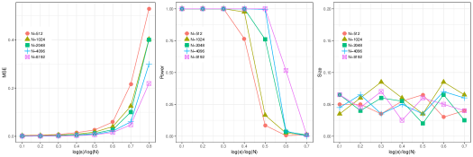
Figure 1: Smoothing Spline Regression. (a) MSE of $\bar{f}$ versus $\rho\equiv\log(s)/\log(N)$. (b) Power of the Wald test versus $\rho$. (c) Size of the Wald test versus $\rho$.

4.2 Nonparametric additive regression

We generated data from the following nonparametric model of two additive components

$$Y_{i}=c*f(X_{i1},X_{i2})+\epsilon_{i},\,\,i=1,\cdots,N,$$ (4.2)

where $f(x_{1},x_{2})=0.4\sin(1.5\pi x_{1})+0.1(0.5-x_{2})^{3}$, and $X_{i1},X_{i2}\overset{iid}{\sim}\text{Unif}[0,1]$, $\epsilon_{i}\overset{iid}{\sim}N(0,1)$, and $c$ is a constant. To examine the estimation procedure, we generated data from (4.2) with $c=1$. To examine the testing procedure, we generated data at $c=0,1$. $N,s$ were chosen to be the same as the smoothing spline example in Section 4. Results are summarized in Figure 2. The interpretations are again similar to Figure 1, only with a slightly different asymptotic trend. Specifically, the MSE suddenly increases at $\rho\approx 0.6$, and the power quickly approaches one at $\rho\approx 0.5$. The sizes are around the nominal level 0.05 for all cases.

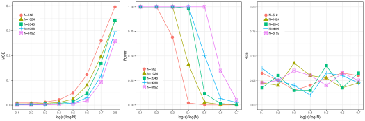
Figure 2: Additive Regression Model. (a) MSE of $\bar{f}$ versus $\rho\equiv\log(s)/\log(N)$. (b) Power of the Wald test versus $\rho$. (c) Size of the Wald test versus $\rho$.

5 Conclusion

Our work offers theoretical insights on how to allocate data in parallel computing for KRR in both estimation and testing procedures. In comparison with [29] and [16], our work provides a general and unified treatment of such problems in modern diverging-dimension or big data settings. Furthermore, using the green function for equivalent kernels to provide a sharp concentration bound on the empirical processes related to $s$, we have improved the upper bound of the number of machines in smoothing spline regression by [29] from $N^{(2m-1)/(2m+1)}/\log{N}$ to $N^{2m/(2m+1)}/\log{N}$ for optimal estimation, which is proven un-improvable in [16] (upto a logarithmic factor). In the end, we would like to point out that our theory is useful in designing a distributed version of generalized cross validation method that is developed to choose tuning parameter $\lambda$ and the number of machines $s$; see [24].

Appendix A Proofs of main results

A.1 Notation table

$N$	sample size
$Y$	response
$X$	covariate
$\epsilon$	random error
$\mathcal{H}$	reproducing kernel Hilbert space (RKHS)
$\pi(x)$	density distribution
$d$	dimension of covariate
$\langle\cdot,\cdot\rangle_{\mathcal{H}}$, $\|\cdot\|_{\mathcal{H}}$	the inner product and norm under $\mathcal{H}$
$R(\cdot,\cdot)$	kernel function under the norm $\|\cdot\|_{\mathcal{H}}$
$\mu_{i}$	eigenvalue
$\varphi$	eigenfunction
$\langle\cdot,\cdot\rangle_{L^{2}_{\pi}(\mathcal{X})}$	$L_{2}$ inner product
$\langle\cdot,\cdot\rangle$, $\|\cdot\|$	embedded inner product and norm
$V(\cdot,\cdot)$	$L_{2}$ inner product
$K(\cdot,\cdot)$	kernel function equipped with $\|\cdot\|$
$K_{x}(\cdot)$	$=K(x,\cdot)$
$s$	number of division
$I_{j}$	the set of indices of the observation from subsample $j$
$n$	the subsample size
$\widehat{f}_{j}$	the estimate of $f$ based on subsample $j$
$\lambda$	penalization parameter
$\bar{f}$	D&C estimator
$T_{N,\lambda}$	test statistic
$\|\cdot\|_{sup}$	the supremum norm
$h^{-1}$	$=\sum_{\nu\geq 1}\frac{1}{1+\lambda/\mu_{\nu}}$
$\xi_{j}$	$=\sup_{\begin{subarray}{c}f,g\in\mathcal{H}\\ \|f\|=\|g\|=1\end{subarray}}|P_{j}fg-Pfg|$
$\mathcal{P}_{\lambda}$	self-adjoint operator satisfies $\langle\mathcal{P}_{\lambda}f,g\rangle=\lambda\langle f,g\rangle_{\mathcal{H}}$
K	empirical kernel matrix
$S^{m}(\mathbb{I})$	the $m$th order Sobolev space on $\mathbb{I}\equiv[0,1]$

Table 2: A table that lists all useful notation and their meanings.

A.2 Some preliminary results

Lemma A.1.

1. For any $x,y\in\mathcal{X}$, $K(x,y)\leq c_{\varphi}^{2}h^{-1}$.

2. For any $f\in\mathcal{H}$, $\|\mathcal{P}_{\lambda}f\|\leq\lambda^{1/2}\|f\|_{\mathcal{H}}$.

Proof.

$(a)$

$$K(x,y)=\sum_{\nu\geq 1}\frac{\varphi_{\nu}(x)\varphi_{\nu}(y)}{1+\lambda/\mu_{\nu}}\leq c_{\varphi}^{2}h^{-1},$$

where the last inequality is by Assumption A3 and the definition of $h^{-1}$.
$(b)$

$$\|\mathcal{P}_{\lambda}f\|= \sup_{g\in\mathcal{H},\|g\|\leq 1}\langle\mathcal{P}_{\lambda}f,g\rangle=\sup_{g\in\mathcal{H},\|g\|\leq 1}\lambda\langle f,g\rangle_{\mathcal{H}}\leq\sup_{g\in\mathcal{H},\|g\|\leq 1}\lambda^{1/2}\|f\|_{\mathcal{H}}\lambda^{1/2}\|g\|_{\mathcal{H}}\leq\lambda^{1/2}\|f\|_{\mathcal{H}}.$$

∎

A.3 Proofs in Section 3.2

Our theoretical analysis relies on a set of Fréchet derivatives to be specified below: for $j=1,2,\ldots,s$, the Fréchet derivative of $\ell_{j,\lambda}$ can be identified as: for any $f,f_{1},f_{2}\in\mathcal{H}$,

$$D\ell_{j,\lambda}(f)f_{1} = -\frac{1}{n}\sum_{i\in I_{j}}(Y_{i}-f(X_{i}))\langle K_{X_{i}},f_{1}\rangle+\langle\mathcal{P}_{\lambda}f,f_{1}\rangle:=\langle S_{j,\lambda}(f),f_{1}\rangle,$$

$$DS_{j,\lambda}(f)f_{1}f_{2} = \frac{1}{n}\sum_{i\in I_{j}}f_{2}(X_{i})\langle K_{X_{i}},f_{1}\rangle+\langle\mathcal{P}_{\lambda}f_{2},f_{1}\rangle=\langle DS_{j,\lambda}(f)f_{2},f_{1}\rangle,$$

$$D^{2}S_{j,\lambda}(f) \equiv 0.$$

More specifically,

$$S_{j,\lambda}(f) = -\frac{1}{n}\sum_{i\in I_{j}}(Y_{i}-f(X_{i}))K_{X_{i}}+\mathcal{P}_{\lambda}f,$$

$$DS_{j,\lambda}(f)g = \frac{1}{n}\sum_{i\in I_{j}}g(X_{i})K_{X_{i}}+\mathcal{P}_{\lambda}g.$$

Define $S_{\lambda}(f)=E\{S_{j,\lambda}(f)\}$, hence, $DS_{\lambda}(f)=E\{DS_{j,\lambda}(f)\}$. It follows from [14] that

$$\langle DS_{\lambda}(f)f_{1},f_{2}\rangle=\langle f_{1},f_{2}\rangle$$

for any $f,f_{1},f_{2}\in\mathcal{H}$ which leads to $DS_{\lambda}(f)=id$.

Proof of Lemma 3.2.

Throughout the proof, let $\widetilde{f}_{j}=E\{\widehat{f}_{j}|\textbf{X}_{j}\}$. It is easy to see that

$$0 = S_{j,\lambda}(\widehat{f}_{j})=-\frac{1}{n}\sum_{i\in I_{j}}(Y_{i}-\widehat{f}_{j}(X_{i}))K_{X_{i}}+\mathcal{P}_{\lambda}\widehat{f}_{j},$$

$$0 = \frac{1}{n}\sum_{i\in I_{j}}(\widetilde{f}_{j}(X_{i})-f_{0}(X_{i}))K_{X_{i}}+\mathcal{P}_{\lambda}\widetilde{f}_{j}.$$

Subtracting the two equations one gets that

$$\frac{1}{n}\sum_{i\in I_{j}}(\widehat{f}_{j}-\widetilde{f}_{j})(X_{i})K_{X_{i}}+\mathcal{P}_{\lambda}(\widehat{f}_{j}-\widetilde{f}_{j})=\frac{1}{n}\sum_{i\in I_{j}}\epsilon_{i}K_{X_{i}}.$$ (A.1)

Equation (A.1) shows that

$$\widehat{f}_{j}-\widetilde{f}_{j}=\mathop{\mathrm{argmin}}_{f\in\mathcal{H}}\ell_{j,\lambda}^{\star}(f)\equiv\mathop{\mathrm{argmin}}_{f\in\mathcal{H}}\frac{1}{2n}\sum_{i\in I_{j}}(\epsilon_{i}-f(X_{i}))^{2}+\frac{\lambda}{2}\|f\|_{\mathcal{H}}^{2}.$$

Let $e_{j}=\frac{1}{n}\sum_{i\in I_{j}}\epsilon_{i}K_{X_{i}}$ and $\varepsilon_{j}=\widehat{f}_{j}-\widetilde{f}_{j}$. Then consider Taylor’s expansion

$$\ell_{j,\lambda}^{\star}(e_{j})-\ell_{j,\lambda}^{\star}(\varepsilon_{j}) = \frac{1}{2}D^{2}\ell_{j,\lambda}^{\star}(\varepsilon_{j})(e_{j}-\varepsilon_{j})(e_{j}-\varepsilon_{j})$$

$$= \frac{1}{2}P_{j}(e_{j}-\varepsilon_{j})^{2}+\frac{1}{2}\langle\mathcal{P}_{\lambda}(e_{j}-\varepsilon_{j}),e_{j}-\varepsilon_{j}\rangle,$$

$$\ell_{j,\lambda}^{\star}(\varepsilon_{j})-\ell_{j,\lambda}^{\star}(e_{j}) = D\ell_{j,\lambda}^{\star}(e_{j})(\varepsilon_{j}-e_{j})+\frac{1}{2}D^{2}\ell_{j,\lambda}^{\star}(e_{j})(\varepsilon_{j}-e_{j})(\varepsilon_{j}-e_{j})$$

$$= (P_{j}-P)(e_{j}(\varepsilon_{j}-e_{j}))+\frac{1}{2}P_{j}(\varepsilon_{j}-e_{j})^{2}+\frac{1}{2}\langle\mathcal{P}_{\lambda}(\varepsilon_{j}-e_{j}),\varepsilon_{j}-e_{j}\rangle.$$

Adding the two equations one obtains that

$$P_{j}(\varepsilon_{j}-e_{j})^{2}+\langle\mathcal{P}_{\lambda}(\varepsilon_{j}-e_{j}),\varepsilon_{j}-e_{j}\rangle+(P_{j}-P)(e_{j}(\varepsilon_{j}-e_{j}))=0.$$

Uniformly for $j$, it holds that

$$|(P_{j}-P)(e_{j}(\varepsilon_{j}-e_{j}))| \leq \xi_{j}\|e_{j}\|\cdot\|\varepsilon_{j}-e_{j}\|,$$

$$P_{j}(\varepsilon_{j}-e_{j})^{2}+\langle\mathcal{P}_{\lambda}(\varepsilon_{j}-e_{j}),(\varepsilon_{j}-e_{j})\rangle \geq (1-\xi_{j})\|\varepsilon_{j}-e_{j}\|^{2}.$$

Combining the two inequalities one gets that

$$(1-\xi_{j})\|\varepsilon_{j}-e_{j}\|^{2}\leq\xi_{j}\|e_{j}\|\cdot\|\varepsilon_{j}-e_{j}\|.$$

Taking expectations conditional on $\textbf{X}_{j}$ on both sides and noting that $\xi_{j}$ is $\sigma(\textbf{X}_{j})$-measurable, one gets that

$$(1-\xi_{j})E\{\|\varepsilon_{j}-e_{j}\|^{2}|\textbf{X}_{j}\}\leq\xi_{j}E\{\|e_{j}\|\cdot\|\varepsilon_{j}-e_{j}\||\textbf{X}_{j}\}\leq\xi_{j}E\{\|e_{j}\|^{2}|\textbf{X}_{j}\}^{1/2}E\{\|\varepsilon_{j}-e_{j}\|^{2}|\textbf{X}_{j}\}^{1/2}.$$

By assumption $\log^{b}{N}=o(nh^{a})$ and Assumption A4, $\max_{1\leq j\leq s}\xi_{j}=o_{P}(1)$, i.e., with probability approaching one $\max_{1\leq j\leq s}\xi_{j}\leq 1/2$, hence,

$$E\{\|\varepsilon_{j}-e_{j}\|^{2}|\textbf{X}_{j}\} \leq 4\xi_{j}^{2}E\{\|e_{j}\|^{2}|\textbf{X}_{j}\}$$ (A.2)

$$= \frac{4\xi_{j}^{2}}{n^{2}}\sum_{i,i^{\prime}\in I_{j}}E\{\epsilon_{i}\epsilon_{i^{\prime}}K(X_{i},X_{i^{\prime}})|\textbf{X}_{j}\}$$

$$= \frac{4\xi_{j}^{2}}{n^{2}}\sum_{i\in I_{j}}\sigma^{2}(X_{i})K(X_{i},X_{i})$$

$$\leq \frac{4c_{\pi}c_{\varphi}^{2}\xi_{j}^{2}}{nh},$$

where the last inequality follows from Assumption A1 and Lemma A.1 that $K(x,x)\leq c_{\varphi}^{2}h^{-1}$. This proves (3.1).

By (A.2) it is easy to derive

$$E\{\|\widehat{f}_{j}-\widetilde{f}_{j}\|^{2}|\textbf{X}_{j}\}\leq\frac{4c_{\pi}c_{\varphi}^{2}}{nh}.$$ (A.3)

Now we look at $\|\widetilde{f}_{j}-f_{0}^{\star}\|$, where $f_{0}^{\star}=(id-\mathcal{P}_{\lambda})f_{0}$. It is easy to see that $\widetilde{f}_{j}$ is the minimizer of the following problem.

$$\widetilde{f}_{j}=\mathop{\mathrm{argmin}}_{f\in\mathcal{H}}\widetilde{\ell}_{j,\lambda}(f)\equiv\mathop{\mathrm{argmin}}_{f\in\mathcal{H}}\frac{1}{2n}\sum_{i\in I_{j}}(f_{0}(X_{i})-f(X_{i}))^{2}+\frac{\lambda}{2}\|f\|_{\mathcal{H}}^{2}.$$

We use a similar strategy for handling part (3.1). Note that

$$\widetilde{\ell}_{j,\lambda}(f_{0}^{\star})-\widetilde{\ell}_{j,\lambda}(\widetilde{f}_{j}) = \frac{1}{2}D^{2}\widetilde{\ell}_{j,\lambda}(\widetilde{f}_{j})(f_{0}^{\star}-\widetilde{f}_{j})(f_{0}^{\star}-\widetilde{f}_{j})$$

$$= \frac{1}{2}P_{j}(f_{0}^{\star}-\widetilde{f}_{j})^{2}+\frac{1}{2}\langle\mathcal{P}_{\lambda}(f_{0}^{\star}-\widetilde{f}_{j}),f_{0}^{\star}-\widetilde{f}_{j}\rangle,$$

$$\widetilde{\ell}_{j,\lambda}(\widetilde{f}_{j})-\widetilde{\ell}_{j,\lambda}(f_{0}^{\star}) = P_{j}(f_{0}^{\star}-f_{0})(\widetilde{f}_{j}-f_{0}^{\star})+\langle\mathcal{P}_{\lambda}f_{0}^{\star},\widetilde{f}_{j}-f_{0}^{\star}\rangle$$

$$+\frac{1}{2}P_{j}(\widetilde{f}_{j}-f_{0}^{\star})^{2}+\frac{1}{2}\langle\mathcal{P}_{\lambda}(\widetilde{f}_{j}-f_{0}^{\star}),\widetilde{f}_{j}-f_{0}^{\star}\rangle.$$

Adding the two equations, one gets that

$$P_{j}(\widetilde{f}_{j}-f_{0}^{\star})^{2}+\langle\mathcal{P}_{\lambda}(\widetilde{f}_{j}-f_{0}^{\star}),\widetilde{f}_{j}-f_{0}^{\star}\rangle$$

$$= P_{j}(f_{0}-f_{0}^{\star})(\widetilde{f}_{j}-f_{0}^{\star})-\langle\mathcal{P}_{\lambda}f_{0}^{\star},\widetilde{f}_{j}-f_{0}^{\star}\rangle$$

$$= (P_{j}-P)(f_{0}-f_{0}^{\star})(\widetilde{f}_{j}-f_{0}^{\star})+P(f_{0}-f_{0}^{\star})(\widetilde{f}_{j}-f_{0}^{\star})-\langle\mathcal{P}_{\lambda}f_{0}^{\star},\widetilde{f}_{j}-f_{0}^{\star}\rangle$$

$$= (P_{j}-P)(f_{0}-f_{0}^{\star})(\widetilde{f}_{j}-f_{0}^{\star})+\langle f_{0}-f_{0}^{\star},\widetilde{f}_{j}-f_{0}^{\star}\rangle$$

$$-\langle\mathcal{P}_{\lambda}(f_{0}-f_{0}^{\star}),\widetilde{f}_{j}-f_{0}^{\star}\rangle-\langle\mathcal{P}_{\lambda}f_{0}^{\star},\widetilde{f}_{j}-f_{0}^{\star}\rangle$$

$$= (P_{j}-P)(f_{0}-f_{0}^{\star})(\widetilde{f}_{j}-f_{0}^{\star})+\langle f_{0}-f_{0}^{\star}-\mathcal{P}_{\lambda}(f_{0}-f_{0}^{\star})-\mathcal{P}_{\lambda}f_{0}^{\star},\widetilde{f}_{j}-f_{0}^{\star}\rangle$$

$$= (P_{j}-P)(f_{0}-f_{0}^{\star})(\widetilde{f}_{j}-f_{0}^{\star}).$$

Therefore,

$$(1-\xi_{j})\|\widetilde{f}_{j}-f_{0}^{\star}\|^{2}\leq\xi_{j}\|f_{0}-f_{0}^{\star}\|\times\|\widetilde{f}_{j}-f_{0}^{\star}\|=\xi_{j}\|\mathcal{P}_{\lambda}f_{0}\|\times\|\widetilde{f}_{j}-f_{0}^{\star}\|\leq C\xi_{j}\lambda^{1/2}\|f_{0}\|_{\mathcal{H}}\|\widetilde{f}_{j}-f_{0}^{\star}\|,$$

implying that, with probability approaching one, for any $1\leq j\leq s$, $\|\widetilde{f}_{j}-f_{0}^{\star}\|\leq 2C\xi_{j}\lambda^{1/2}\|f_{0}\|_{\mathcal{H}}$. This proves (3.2). ∎

Proof of Theorem 3.3.

Recall $f_{0}^{\star}=(id-\mathcal{P}_{\lambda})f_{0}$ and $\widetilde{f}_{j}=E\{\widehat{f}_{j}|\textbf{X}_{j}\}$. Also notice that $\frac{1}{N}\sum_{i=1}^{N}\epsilon_{i}K_{X_{i}}=\frac{1}{s}\sum_{j=1}^{s}e_{j}$. By direct calculations and Lemma 3.2, we have with probability approaching one,

$$E\{\|\bar{f}-f_{0}^{\star}-\frac{1}{N}\sum_{i=1}^{N}\epsilon_{i}K_{X_{i}}\|^{2}|\textbf{X}\}$$

$$= \frac{1}{s^{2}}\sum_{j=1}^{s}E\{\|\widehat{f}_{j}-\widetilde{f}_{j}-e_{j}\|^{2}|\textbf{X}_{j}\}+\frac{1}{s^{2}}\|\sum_{j=1}^{s}(\widetilde{f}_{j}-f_{0}^{\star})\|^{2}$$

$$\leq 4\left(\frac{c_{\pi}c_{\varphi}^{2}}{Nh}+\lambda\|f_{0}\|_{\mathcal{H}}^{2}\right)\max_{1\leq j\leq s}\xi_{j}^{2}.$$

This proves (3.3). The result (3.4) immediately follows by the assumption $\max_{1\leq j\leq s}\xi_{j}^{2}=o_{P}(1)$. ∎

A.4 Proofs in Section 3.3

Proof of Lemma 3.4.

It is easy to see that

$$\bm{\epsilon}^{\prime}\textbf{K}\bm{\epsilon}=\sum_{i=1}^{N}\epsilon_{i}^{2}K(X_{i},X_{i})+W(N).$$

Since

$$Var\left(\sum_{i=1}^{N}\epsilon_{i}^{2}K(X_{i},X_{i})\right)\leq NE\{\epsilon_{i}^{4}K(X_{i},X_{i})^{2}\}\leq\tau c_{\varphi}^{4}Nh^{-2},$$

where the last “$\leq$” follows by Assumption A2 and Lemma A.1 that $K(x,x)\leq c_{\varphi}^{2}h^{-1}$, we get that

$$\sum_{i=1}^{N}\epsilon_{i}^{2}K(X_{i},X_{i}) = E\{\sum_{i=1}^{N}\epsilon_{i}^{2}K(X_{i},X_{i})\}+O_{P}\left(\sqrt{c_{\varphi}^{4}Nh^{-2}}\right)$$

$$= \sigma^{2}Nh^{-1}+O_{P}(\sqrt{c_{\varphi}^{4}Nh^{-2}}).$$

Next we prove asymptotic normality of $W(N)$. Note $\sigma^{2}(N)=E\{W(N)^{2}\}$. Let $G_{I}$, $G_{II}$, $G_{IV}$ be defined as

$$G_{I} = \sum_{1\leq i<t\leq n}E\{W_{it}^{4}\},$$

$$G_{II} = \sum_{1\leq i<t<k\leq n}(E\{W_{it}^{2}W_{ik}^{2}\}+E\{W_{ti}^{2}W_{tk}^{2}\}+E\{W_{ki}^{2}W_{kt}^{2}\})$$

$$G_{IV} = \sum_{1\leq i<t<k<l\leq n}(E\{W_{it}W_{ik}W_{lt}W_{lk}\}+E\{W_{it}W_{il}W_{kt}W_{kl}\}+E\{W_{ik}W_{il}W_{tk}W_{tl}\}).$$

Since $K(x,x)\leq c_{\varphi}^{2}h^{-1}$, we have $G_{I}=O(N^{2}h^{-4})$ and $G_{II}=O(N^{3}h^{-4})$. It can also be shown that for pairwise distinct $i,k,t,l$,

$$E\{W_{ik}W_{il}W_{tk}W_{tl}\}$$

$$= 2^{4}E\{\epsilon_{i}^{2}\epsilon_{k}^{2}\epsilon_{t}^{2}\epsilon_{l}^{2}K(X_{i},X_{k})K(X_{i},X_{l})K(X_{t},X_{k})K(X_{t},X_{l})\}$$

$$= 2^{4}\sigma^{8}\sum_{\nu=1}^{\infty}\frac{1}{(1+\lambda/\mu_{\nu})^{4}}=O(h^{-1}),$$

which implies that $G_{IV}=O(N^{4}h^{-1})$. In the mean time, a straight algebra leads to that

$$\sigma^{2}(N) = 4\sigma^{4}{N\choose 2}\sum_{\nu=1}^{\infty}\frac{1}{(1+\lambda/\mu_{\nu})^{2}}$$

$$= 2\sigma^{4}N(N-1)\sum_{\nu\geq 1}\frac{1}{(1+\lambda/\mu_{\nu})^{2}}\asymp N^{2}h^{-1},$$

where the last conclusion follows by Proposition 3.1. Thanks to the conditions $h\to 0$, $Nh^{2}\to\infty$, $G_{I},G_{II}$ and $G_{IV}$ are all of order $o(\sigma^{4}(N))$. Then it follows by [2] that as $N\rightarrow\infty$,

$$\frac{W(N)}{\sigma(N)}\overset{d}{\longrightarrow}N(0,1).$$

The above limit leads to that $W(N)=O_{P}(Nh^{-1/2})$. ∎

Proof of Theorem 3.5.

The proof is based on Lemma 3.4. Under $f_{0}=0$, it follows from Corollary 3.3 and Assumption A4 that

$$E\{\|\bar{f}-\frac{1}{N}\sum_{i=1}^{N}\epsilon_{i}K_{X_{i}}\|^{2}|\textbf{X}\}=O_{P}\left(\frac{c_{\varphi}^{2}\log^{b}{N}}{Nnh^{1+a}}\right),$$

leading to

$$\|\bar{f}-\frac{1}{N}\sum_{i=1}^{N}\epsilon_{i}K_{X_{i}}\|^{2}=O_{P}\left(\frac{c_{\varphi}^{2}\log^{b}{N}}{Nnh^{1+a}}\right).$$

Following the proof of Lemma 3.2 and the trivial fact $\widehat{f}_{j}=0$ when $f_{0}=0$, we have for any $1\leq j\leq s$,

$$E\{\|\widehat{f}_{j}-e_{j}\|^{2}|\textbf{X}_{j}\}\leq\frac{4c_{\pi}c_{\varphi}^{2}\xi_{j}^{2}}{nh},\,\,\,\,E\{\|e_{j}\|^{2}|\textbf{X}_{j}\}\leq\frac{c_{\pi}c_{\varphi}^{2}}{nh},\,\,\,\,\textrm{a.s.}$$ (A.4)

Therefore, by Cauchy-Schwartz inequality,

$$E\{|\langle\widehat{f}_{j}-e_{j},e_{j}\rangle|\big{|}\textbf{X}_{j}\}\leq\sqrt{E\{\|\widehat{f}_{j}-e_{j}\|^{2}|\textbf{X}_{j}\}E\{\|e_{j}\|^{2}|\textbf{X}_{j}\}}\leq\frac{2c_{\pi}c_{\varphi}^{2}}{nh}\xi_{j},$$

and hence,

$$E\left\{\sum_{j=1}^{s}|\langle\widehat{f}_{j}-e_{j},e_{j}\rangle|\bigg{|}\textbf{X}\right\}\leq\frac{2c_{\pi}sc_{\varphi}^{2}}{nh}\max_{1\leq j\leq s}\xi_{j}.$$

By Assumption A4, the above leads to that

$$\sum_{j=1}^{s}\langle\widehat{f}_{j}-e_{j},e_{j}\rangle=O_{P}\left(\frac{sc_{\varphi}^{2}}{nh}\sqrt{\frac{\log^{b}{N}}{nh^{a}}}\right).$$

Meanwhile, it holds that

$$\sum_{j\neq l}\langle\widehat{f}_{j}-e_{j},e_{l}\rangle=\sum_{j<l}\langle\widehat{f}_{j}-e_{j},e_{l}\rangle+\sum_{j>l}\langle\widehat{f}_{j}-e_{j},e_{l}\rangle\equiv R_{1}+R_{2},$$

with

$$R_{1}=O_{P}\left(\frac{sc_{\varphi}^{2}}{nh}\sqrt{\frac{\log^{b}{N}}{nh^{a}}}\right),\,\,\,\,R_{2}=O_{P}\left(\frac{sc_{\varphi}^{2}}{nh}\sqrt{\frac{\log^{b}{N}}{nh^{a}}}\right).$$

To see this, note that

$$E\{R_{1}^{2}|\textbf{X}\} = \sum_{j<l}E\{|\langle\widehat{f}_{j}-e_{j},e_{l}\rangle|^{2}|\textbf{X}\}$$

$$\leq \sum_{j<l}E\{\|\widehat{f}_{j}-e_{j}\|^{2}\|e_{l}\|^{2}|\textbf{X}\}$$

$$= \sum_{j<l}E\{\|\widehat{f}_{j}-e_{j}\|^{2}|\textbf{X}_{j}\}E\{\|e_{l}\|^{2}|\textbf{X}_{l}\}$$

$$\leq {s\choose 2}\frac{4c_{\pi}^{2}c_{\varphi}^{4}}{n^{2}h^{2}}\max_{1\leq j\leq s}\xi_{j}^{2},$$

where the last inequality is based on (A.4). Similar result holds for $R_{2}$. Hence, by Lemma 3.4 and direct algebra, we get that

$$T_{N,\lambda} = N^{-2}\bm{\epsilon}^{\prime}\textbf{K}\bm{\epsilon}+\frac{2}{s^{2}}\sum_{j,l=1}^{s}\langle\widehat{f}_{j}-e_{j},e_{l}\rangle+\|\bar{f}-\frac{1}{N}\sum_{i=1}^{N}\epsilon_{i}K_{X_{i}}\|^{2}$$

$$= N^{-2}\bm{\epsilon}^{\prime}\textbf{K}\bm{\epsilon}+\frac{2}{s^{2}}\sum_{j=1}^{s}\langle\widehat{f}_{j}-e_{j},e_{j}\rangle+\frac{2}{s^{2}}(R_{1}+R_{2})+\|\bar{f}-\frac{1}{N}\sum_{i=1}^{N}\epsilon_{i}K_{X_{i}}\|^{2}$$

$$= \frac{\sigma^{2}}{Nh}+\frac{W(N)}{N^{2}}+O_{P}\left(\frac{c_{\varphi}^{2}}{N^{3/2}h}\right)+O_{P}\left(\frac{c_{\varphi}^{2}}{Nh}\sqrt{\frac{\log^{b}{N}}{nh^{a}}}\right)+O_{P}\left(\frac{c_{\varphi}^{2}\log^{b}{N}}{Nnh^{1+a}}\right)$$

$$= \frac{\sigma^{2}}{Nh}+\frac{W(N)}{N^{2}}+O_{P}\left(\frac{c_{\varphi}^{2}}{N^{3/2}h}\right)+O_{P}\left(\frac{c_{\varphi}^{2}}{Nh}\sqrt{\frac{\log^{b}{N}}{nh^{a}}}\right).$$

The last equality follows from the condition $\log^{b}{N}=o(nh^{a+1})$. Therefore, by $c_{\varphi}^{4}/(Nh)=o(1)$, $Nh\to\infty$ (from $Nh^{2}\to\infty$ and $h\to 0$), condition $\log^{b}{N}=o(nh^{a+1})$ and $\sigma^{2}(N)\asymp N^{2}h^{-1}$ (Lemma 3.4), as $N\to\infty$,

$$\frac{N^{2}}{\sigma(N)}\left(T_{N,\lambda}-\frac{\sigma^{2}}{Nh}\right) = \frac{W(N)}{\sigma(N)}+O_{P}\left(\frac{c_{\varphi}^{2}}{\sqrt{Nh}}+c_{\varphi}^{2}\sqrt{\frac{\log^{b}{N}}{nh^{a+1}}}\right)$$

$$= \frac{W(N)}{\sigma(N)}+o_{P}(1)\overset{d}{\to}N(0,1).$$

Proof is completed. ∎

Proof of Theorem 3.6.

For any $f\in\mathcal{H}$, define $R_{f}=\bar{f}-N^{-1}\sum_{i=1}^{N}\epsilon_{i}K_{X_{i}}-f+\mathcal{P}_{\lambda}f$. By direct examinations, it holds that

$$\|\bar{f}\|^{2}-\sigma^{2}/(Nh)$$

$$= \|R_{f}+\frac{1}{N}\sum_{i=1}^{N}\epsilon_{i}K_{X_{i}}+f-\mathcal{P}_{\lambda}f\|^{2}-\sigma^{2}/(Nh)$$

$$\geq \left\{\bm{\epsilon}^{\prime}\textbf{K}\bm{\epsilon}/N^{2}-\sigma^{2}/(Nh)\right\}+\|f-\mathcal{P}_{\lambda}f\|^{2}-\frac{2}{N}\sum_{i=1}^{N}\epsilon_{i}(f-\mathcal{P}_{\lambda}f)(X_{i})$$

$$+\frac{2}{N}\sum_{i=1}^{N}\epsilon_{i}R_{f}(X_{i})-2\langle f-\mathcal{P}_{\lambda}f,R_{f}\rangle$$

$$\equiv T_{1}+T_{2}+T_{3}+T_{4}+T_{5}.$$

It follows by (3.5), Theorem 3.3, Assumption A4 that, uniformly for $f\in\mathcal{H}$,

$$T_{1}=W(N)/N^{2}+O_{P}((N^{3/2}h)^{-1}),\,\,\,\,\textrm{(by (\ref{basic:lemma:for:testing:eqn:0}))}$$

$$P_{f}\left(|T_{3}|\geq\sigma\|f-\mathcal{P}_{\lambda}f\|/(\varepsilon\sqrt{N})\right)\leq\varepsilon^{2},\,\,\,\,\textrm{for arbitrary $\varepsilon>0$}$$

$$T_{4}=O_{P}(b_{N,\lambda}/\sqrt{Nh}),\,\,\,\,\textrm{(by Theorem \ref{thm:of:thm1}, Assumption \ref{A4} and (\ref{basic:lemma:for:testing:eqn:0}))}$$

$$T_{5}=\|f-\mathcal{P}_{\lambda}f\|\times O_{P}(b_{N,\lambda}),\,\,\,\,\textrm{(by Theorem \ref{thm:of:thm1} and Assumption \ref{A4})}$$

Note that $\|\mathcal{P}_{\lambda}f\|\leq\lambda^{1/2}\|f\|_{\mathcal{H}}$ for any $f\in\mathcal{H}$. Therefore, to achieve high power, i.e., power is at least $1-\varepsilon$, one needs to choose a large $N_{\varepsilon}$ and $C_{\varepsilon}$ s.t. $N\geq N_{\varepsilon}$ and

$$\|f\|\geq C_{\varepsilon}/\sqrt{Nh^{1/2}},\,\,\,\,\|f\|\geq C_{\varepsilon}/\sqrt{N},\,\,\,\,\|f\|\geq C_{\varepsilon}\sqrt{b_{N,\lambda}/\sqrt{Nh}},\,\,\,\,$$

$$\|f\|\geq C_{\varepsilon}b_{N,\lambda},\,\,\,\,\|f\|\geq C_{\varepsilon}\lambda^{1/2}\|f\|_{\mathcal{H}}.$$

Proof is completed. ∎

A.5 Proofs in Section 3.4.2

Proof of Lemma 3.9 $(\ref{le:add:prelim:a})$.

For each $\nu\geq 1$, there exist $p\in\mathbb{N}$ and $1\leq k\leq d$, such that $\nu=pd+k$. Suppose $x=(x_{1},\cdots,x_{d})$, then for each $x_{k}$, there exists $(\varphi_{p}^{(k)},\mu_{p}^{(k)})$ and $(\varphi_{p^{\prime}}^{(k)},\mu_{p^{\prime}}^{(k)})$ satisfying $V_{k}(\varphi_{p}^{(k)},\varphi_{p^{\prime}}^{(k)})=\delta_{pp^{\prime}}$ and $\int_{\mathbb{I}}\varphi_{p}^{(k)}(x)\varphi_{p^{\prime}}^{(k)}(x)dx=\delta_{pp^{\prime}}/\mu_{p}^{(k)}$. In fact, the eigenfunctions $\varphi_{\nu}$ and eigenvalues $\mu_{\nu}$ can be constructed by an ordered sequence of $\varphi_{p}^{(k)},\mu_{p}^{(k)}$ as $\varphi_{\nu}(x)=\varphi_{p}^{(k)}(x_{k})$ and $\mu_{\nu}=\mu_{p}^{(k)}$.

Next, we verify such construction of eigenfunctions $\varphi_{\nu}$ and eigenvalues $\mu_{\nu}$ satisfy Assumption A3. When $\nu\neq\mu$, then there exist $p_{1},q_{1},p_{2},q_{2}$, such that $\nu=p_{1}d+q_{1},\mu=p_{2}d+q_{2}$, then

$$V(\varphi_{p_{1}d+q_{1}},\varphi_{p_{2}d+q_{2}}) =V(\varphi_{p_{1}}^{q_{1}}(x_{q_{1}}),\varphi_{p_{2}}^{q_{2}}(x_{q_{2}}))$$

$$=\begin{cases}0&\quad p_{1}\neq p_{2},q_{1}=q_{2}\\ V_{q_{1}}(\varphi_{p_{1}}^{q_{1}}(x_{q_{1}}),0)+V_{q_{2}}(0,\varphi_{p_{2}}^{q_{2}}(x_{q_{2}}))=0&\quad q_{1}\neq q_{2}\\ \end{cases}$$

On the other hand,

$$\langle\varphi_{\nu},\varphi_{\mu}\rangle_{\mathcal{H}}=\langle\varphi_{p_{1}}^{q_{1}},\varphi_{p_{2}}^{q_{2}}\rangle_{\mathcal{H}}=\begin{cases}1/\mu_{p_{1}}^{q_{1}}=1/\mu_{\nu}&\quad p_{1}=p_{2},q_{1}=q_{2}\\ 0&\quad\nu\neq\mu\\ \end{cases}$$

For any $f\in\mathcal{H}$,

$$f(x_{1},\cdots,x_{d}) =f_{1}(x_{1})+\cdots+f_{d}(x_{d})=\sum_{k=1}^{d}\sum_{\nu=1}^{\infty}V_{k}(f_{k},\varphi_{\nu}^{(k)})\varphi_{\nu}^{(k)}(x_{k})$$

$$=\sum_{k=1}^{d}\sum_{\nu=1}^{\infty}V(f,\varphi_{\nu}^{(k)})\varphi_{\nu}^{(k)}(x_{k})=\sum_{\nu=1}^{\infty}V(f,\varphi_{\nu})\varphi_{\nu}(x)$$

∎

Proof of Lemma 3.9 $(\ref{le:add:prelim:b})$.

It is easy to see that

$$\sum_{\nu\geq 1}(1+\lambda/\mu_{\nu})^{-1}=\sum_{q=1}^{d}\sum_{p\geq 1}(1+\lambda/\mu_{p}^{(k)})^{-1}\asymp d\lambda^{-1/(2m)}:=h^{-1}.$$

∎

Proof of Lemma 3.9 $(\ref{le:add:prelim:c})$.

Notice that $\|f\|^{2}_{\mathcal{H}}\leq\sum_{i=1}^{d}\|f_{k}\|^{2}_{\mathcal{H}}\leq Cd$, then by Lemma A.1 $(b)$, $\|\mathcal{P}_{\lambda}f\|^{2}\leq\lambda\|f\|^{2}_{\mathcal{H}}\leq Cd\lambda$. ∎

Next, we prove Lemma 3.9 (4). To prove Lemma 3.9 (4), it is sufficient to prove the following Lemma A.2.

Lemma A.2.

Under (3.7), there exist universal positive constants $c_{1},c_{2},c_{3}$ such that for any $1\leq j\leq s$,

$$P\left(\xi_{j}\geq t\right)\leq 2n\exp\left(-\frac{nht^{2}}{c_{1}+c_{2}t}\right),\,\,\textrm{for all $t\geq c_{3}(nh)^{-1}$},$$

where $h^{-1}\asymp d\lambda^{-1/(2m)}$.

The proof of Lemma 3.9 is based on the green function for equivalent kernel technique in [3], see Supplement for details.

A.6 Proofs in Section 3.4

Proof of Lemma 3.11.

For $p,\delta>0$, define $\mathcal{G}(p)=\{f\in\mathcal{H}:\|f\|_{\sup}\leq 1,\|f\|_{\mathcal{H}}\leq p\}$ and the corresponding entropy integral

$$J(p,\delta)=\int_{0}^{\delta}\psi_{2}^{-1}\left(D(\varepsilon,\mathcal{G}(p),\|\cdot\|_{\sup})\right)d\varepsilon+\delta\psi_{2}^{-1}\left(D(\delta,\mathcal{G}(p),\|\cdot\|_{\sup})^{2}\right),$$ (A.5)

where $\psi_{2}(s)=\exp(s^{2})-1$ and $D(\varepsilon,\mathcal{G}(p),\|\cdot\|_{\sup})$ is the $\varepsilon$-packing number of $\mathcal{G}(p)$ in terms of $\|\cdot\|_{\sup}$-metric. In what follows, we particularly choose $p=c_{K}^{-1}(h/\lambda)^{1/2}$, where $c_{K}\equiv\sup_{g\in\mathcal{H}}h^{1/2}\|g\|_{\sup}/\|g\|$ is finite, according to [26].

Define $\psi_{i}(g)=c_{k}^{-1}h^{1/2}g(X_{i})$ and $Z_{j}(g)=n^{-1/2}\sum_{i\in I_{j}}[\psi_{i}(g)K_{X_{i}}-E\{\psi_{i}(g)K_{X_{i}}\}]$. Following [26, Lemma 6.1], for any $1\leq j\leq s$, for any $t\geq 0$,

$$P\left(\sup_{g\in\mathcal{G}(p)}\|Z_{j}(g)\|\geq t\right)\leq 2\exp\left(-\frac{t^{2}}{C^{2}J(p,1)^{2}}\right),$$ (A.6)

for an absolute constant $C>0$. Since $\|f\|=1$ implies that $c_{K}^{-1}h^{1/2}f\in\mathcal{G}(p)$. Then it can be shown that

$$\sqrt{n}\xi_{j}\leq c_{K}^{2}h^{-1}\sup_{g\in\mathcal{G}(p)}\|Z_{j}(g)\|,\,\,\,\,j=1,\ldots,s.$$

Following (A.6) we have

$$P\left(\sqrt{n}\max_{1\leq j\leq s}\xi_{j}\geq t\right)\leq 2s\exp\left(-\frac{c_{K}^{-4}h^{2}t^{2}}{C^{2}J(p,1)^{2}}\right),$$

which implies that

$$\sqrt{n}\max_{1\leq j\leq s}\xi_{j}=O_{P}\left(\sqrt{\frac{\log{N}}{h^{2}}}J(p,1)\right).$$ (A.7)

It follows by [30, Proposition 1] that $J(p,1)=O\left([\log(h/\lambda)]^{(d+1)/2}\right)=O\left([\log{N}]^{(d+1)/2}\right)$. Then

$$\max_{1\leq j\leq s}\xi_{j}=O_{P}\left(\sqrt{\frac{\log^{d+2}{N}}{nh^{2}}}\right).$$

That is, Assumption A4 holds with $a=2$ and $b=d+2$. Proof completed. ∎

Proof of Lemma 3.13.

$$J(p,1) \leq\int_{0}^{1}\sqrt{\log D(\varepsilon,\mathcal{G},\|\cdot\|_{\sup})}\,d\varepsilon+\sqrt{\log D(1,\mathcal{G},\|\cdot\|_{\sup})}$$

$$\leq\int_{0}^{1}\sqrt{\left(\frac{p}{\varepsilon}\right)^{\frac{d}{m}}+1}\,d\varepsilon+\sqrt{2}p^{\frac{d}{2m}}$$

$$\leq c^{\prime}_{d}\,p^{d/(2m)}$$

where the penultimate step is based on [12]. Therefore, $J(p,1)=O(p^{\frac{d}{2m}})$, where $p=(h/\lambda)^{1/2}$. From e.q.(A.7), we have

$$\max_{1\leq j\leq s}\xi_{j}=O_{P}\left(\sqrt{\frac{\log N}{nh^{3-d/(2m)}}}\right)$$

∎

Appendix B Some technical proofs

B.1 Proof of Proposition 3.1

Proof.

Define

$$s_{\lambda}=\mathop{\mathrm{argmin}}\{j:\mu_{j}\leq\lambda\}-1,$$

that is, $s_{\lambda}$ is the number of eigenvalues that are greater than $\lambda$. Then the effective dimension can be written as

$$h^{-1}=\sum_{j=1}^{\infty}\frac{\mu_{j}}{\mu_{j}+\lambda}=\sum_{j=1}^{s_{\lambda}}\frac{\mu_{j}}{\mu_{j}+\lambda}+\sum_{j=s_{\lambda}+1}^{\infty}\frac{\mu_{j}}{\mu_{j}+\lambda}.$$

Note that $\sum_{j=1}^{s_{\lambda}}\mu_{j}/(\mu_{j}+\lambda)\leq s_{\lambda}$, then we have

$$s_{\lambda}\leq h^{-1}\leq s_{\lambda}+\sum_{j=s_{\lambda}+1}^{\infty}\frac{\mu_{j}}{\mu_{j}+\lambda}\leq s_{\lambda}+\frac{1}{\lambda}\sum_{j=s_{\lambda}+1}^{\infty}\mu_{j}.$$ (B.1)

By Assumption 3.3, we have $\sum_{j=s_{\lambda}+1}^{\infty}\mu_{j}\leq Cs_{\lambda}\mu_{s_{\lambda}}\leq s_{\lambda}\lambda$. Therefore, by (B.1), we have $h^{-1}\asymp s_{\lambda}$. Next we show $\sum_{\nu\geq 1}(1+\lambda/\mu_{\nu})^{-2}\asymp h^{-1}$.

Note that

$$\sum_{\nu\geq 1}(1+\lambda/\mu_{\nu})^{-2}=\sum_{j=1}^{\infty}\frac{\mu_{j}^{2}}{(\mu_{j}+\lambda)^{2}}=\sum_{j=1}^{s_{\lambda}}\big{(}\frac{\mu_{j}}{\mu_{j}+\lambda}\big{)}^{2}+\sum_{j=s_{\lambda}+1}^{\infty}\big{(}\frac{\mu_{j}}{\mu_{j}+\lambda}\big{)}^{2},$$

similar to (B.1), we have

$$s_{\lambda}\leq\sum_{\nu\geq 1}(1+\lambda/\mu_{\nu})^{-2}\leq s_{\lambda}+\sum_{j=s_{\lambda}+1}^{\infty}\big{(}\frac{\mu_{j}}{\mu_{j}+\lambda}\big{)}^{2}\leq s_{\lambda}+\frac{1}{\lambda^{2}}\sum_{j=s_{\lambda}+1}^{\infty}\mu_{j}^{2}.$$

Since $\frac{1}{\lambda^{2}}\sum_{j=s_{\lambda}+1}^{\infty}\mu_{j}^{2}\leq\frac{\mu_{s_{\lambda}+1}}{\lambda^{2}}\sum_{j=s_{\lambda}+1}^{\infty}\mu_{j}\leq\frac{1}{\lambda}\sum_{j=s_{\lambda}+1}^{\infty}\mu_{j}\leq s_{\lambda}$. Then we have $\sum_{\nu\geq 1}(1+\lambda/\mu_{\nu})^{-2}\asymp s_{\lambda}$. Based on the previous conclusion that $h^{-1}\asymp s_{l}ambda$, we finally get $\sum_{\nu\geq 1}(1+\lambda/\mu_{\nu})^{-2}\asymp h^{-1}$. ∎

B.2 Verification of Assumption 3.3

Let us verify Assumption 3.3 in polynomially decaying kernels (PDK) and exponentially decaying kernels (EDK).

First consider PDK with $\mu_{i}\asymp i^{-2m}$ for a constant $m>1/2$ which includes kernels of Sobolev space and Besov Space. An $m$-th order Sobolev space, denoted $\mathcal{H}^{m}([0,1])$, is defined as

$$\mathcal{H}^{m}([0,1])= \{f:[0,1]\to\mathbb{R}|f^{(j)}\;\;\text{is abs. cont for}\;j=0,1,\cdots,m-1,$$

$$\text{and}\;f^{m}\in L_{2}([0,1])\}.$$

An $m$-order periodic Sobolev space, denoted $H_{0}^{m}(\mathbb{I})$, is a proper subspace of $\mathcal{H}^{m}([0,1])$ whose element fulfills an additional constraint $g^{(j)}(0)=g^{(j)}(1)$ for $j=0,\ldots,m-1$. The basis functions $\varphi_{i}$’s of $H_{0}^{m}(\mathbb{I})$ are

$$\varphi_{i}(z)=\left\{\begin{array}[]{cc}\sigma,&i=0,\\ \sqrt{2}\sigma\cos(2\pi kz),&i=2k,k=1,2,\ldots,\\ \sqrt{2}\sigma\sin(2\pi kz),&i=2k-1,k=1,2,\ldots.\end{array}\right.$$

The corresponding eigenvalues are $\mu_{2k}=\mu_{2k-1}=\sigma^{2}(2\pi k)^{-2m}$ for $k\geq 1$ and $\mu_{0}=\infty$. In this case, $\sup_{i\geq 1}\|\varphi\|_{\sup}<\infty$. For any $k\geq 1$,

$$\sum_{i=k+1}^{\infty}\mu_{i}\lesssim\int_{k}^{\infty}x^{-2m}dx=\frac{k^{1-2m}}{2m-1}\lesssim\frac{k\mu_{k}}{2m-1}.$$

Therefore, there exists a constant $C<\infty$, such that

$$\sup_{k\geq 1}\frac{\sum_{i=k+1}^{\infty}\mu_{i}}{k\mu_{k}}=C<\infty.$$

Hence, Assumption 3.3 holds true.

Next, let us consider EDK with $\mu_{i}\asymp\exp(-\gamma i^{p})$ for constants $\gamma>0$ and $p>0$. Gaussian kernel $K(x,x^{\prime})=\exp\left(-(x-x^{\prime})^{2}/\sigma^{2}\right)$ is an EDK of order $p=2$, with eigenvalues $\mu_{i}\asymp\exp(-\pi i^{2})$ as $i\to\infty$, and the corresponding eigenfunctions

$$\varphi_{i}(x)=(\sqrt{5}/4)^{1/4}(2^{i-1}i!)^{-1/2}e^{-(\sqrt{5}-1)x^{2}/4}H_{i}((\sqrt{5}/2)^{1/2}x),$$

where $H_{i}(\cdot)$ is the $i$-th Hermite polynomial; see [17] for more details. Then $\sup_{i\geq 1}\|\varphi_{i}\|_{\sup}<\infty$ trivially holds. For any $k\geq 1$,

$$\sum_{i=k+1}^{\infty}\mu_{i}\lesssim\int_{k}^{\infty}e^{-\gamma x^{p}}dx\\ =\frac{1}{\gamma pk^{p-1}}e^{-\gamma k^{p}}-\int_{k}^{\infty}\frac{p-1}{\gamma px^{p}}e^{-\gamma x^{p}}dx\leq\frac{1}{\gamma pk^{p-1}}e^{-\gamma k^{p}}.$$

Therefore,

$$\sup_{k\geq 1}\frac{\sum_{i=k+1}^{\infty}\mu_{i}}{k\mu_{k}}<\infty.$$

Hence, Assumption 3.3 holds.

B.3 Proof of Lemma A2

To prove Lemma A2, based on Lemma 3.5 and Lemma 3.4 in Chapter 21 in [3], we only need to bound

$$\|\frac{1}{n}\sum_{i=1}^{n}K_{h}(X_{i},\cdot)-\operatorname{E}[K_{h}(X_{i}),\cdot]\|_{\infty},$$

$$\textrm{and}\quad\|\frac{1}{n}\sum_{i=1}^{n}hK_{h}^{\prime}(X_{i},\cdot)-h\operatorname{E}[K_{h}^{\prime}(X_{i}),\cdot]\|_{\infty}.$$

Lemma 1.

Assume that the family $K_{h}=\sum_{j=1}^{d}K_{h_{0},j}$ with $K_{h_{0},j}$, $0<h_{0}\leq 1$ is convolution-like. Then there exists a constant $c$, such that,for all $h$, $0<h\leq 1$, and for every strictly positive design $X_{1},X_{2},\cdots,X_{n}\in(0,1]^{d}$,

$$\|\frac{1}{n}\sum_{i=1}^{n}K_{h}(X_{i},\cdot)\|_{\infty}\leq c\|\frac{1}{n}\sum_{i=1}^{n}g_{h}(X_{i}-\cdot)\|_{\infty}.$$

Proof.

For $t=(t_{1},\cdots,t_{d})\in[0,1]^{d}$ and $x=(x_{1},\cdots,x_{d})\in[0,1]^{d}$, let $S_{nh}(t)=\frac{1}{n}\sum_{i=1}^{n}K_{h}(X_{i},t)$, and $s^{nh}(t)=\frac{1}{n}\sum_{i=1}^{n}g_{h}(X_{i}-t)$. For $j=1,\cdots,d$, $K_{h,j}$ satisfies

$$K_{h_{0},j}(t_{j},x_{j})=h_{0}g_{h,j}(x)K_{h_{0},j}(t_{j},0)+\int_{0}^{1}g_{h_{0},j}(x_{j}-z_{j})\{h_{0}K^{\prime}_{h_{0},j}(t_{j},z_{j})+K_{h_{0},j}(t_{j},z_{j})\}dz_{j},$$

where $h_{0}=dh$. Note that $K_{h_{0},j}$, $h_{0}K_{h_{0},j}^{\prime}$ are all convolutional-like, then $|h_{0}K^{\prime}_{h_{0},j}(t_{j},z_{j})|\leq ch_{0}^{-1}$ and $|K_{h_{0},j}(t_{j},z_{j})|\leq ch_{0}^{-1}$. Therefore,

$$\int_{0}^{1}g_{h_{0},j}(x_{j}-z_{j})\{h_{0}K^{\prime}_{h_{0},j}(t_{j},z_{j})+K_{h_{0},j}(t_{j},z_{j})\}dz_{j}\leq 2c\cdot h_{0}^{-1}\int_{0}^{1}g_{h_{0},j}(x_{j}-z_{j})dz_{j}$$

$$= 2c\cdot h_{0}^{-2}\int_{0}^{1}e^{-h_{0}^{-1}(x_{j}-z_{j})}dz_{j}\leq 2c\cdot\big{(}g_{h_{0},j}(x_{j})-g_{h_{0},j}(x_{j}-1)\big{)}\leq 2c\cdot g_{h_{0},j}(x_{j}).$$

Then, we have $K_{h_{0},j}(t_{j},x_{j})\leq h_{0}\cdot g_{h_{0},j}(x)K_{h_{0},j}(t_{j},0)+c\cdot g_{h_{0},j}(x_{j})$.

$$K_{h}(x,t)= \sum_{j=1}^{d}K_{h_{0},j}(t_{j},x_{j})\leq h_{0}\sum_{j=1}^{d}g_{h_{0},j}(x_{j})K_{h_{0},j}(t_{j},0)+c\sum_{j=1}^{d}g_{h_{0},j}(x_{j})$$

$$\leq c_{1}\sum_{j=1}^{d}g_{h_{0},j}(x_{j})+c\sum_{j=1}^{d}g_{h_{0},j}(x_{j})\leq c^{\prime}\sum_{j=1}^{d}g_{h_{0},j}(x_{j})=c^{\prime}g_{h}(x),$$

where $c_{1}=\max\{h_{0}K_{h_{0},1}(t_{1},0),\cdots,h_{0}K_{h_{0},d}(t_{d},0)\}$ is a bounded constant by the convolution-like assumption. Let $X_{i}=x$ and substitute the formula above into the expression for $S_{nh}(t)$ and $s^{nh}(t)$, this gives $S_{nh}(t)\leq c^{\prime}s^{nh}(0)$. Therefore, $\|S_{nh}\|_{\infty}\leq c^{\prime}|s^{nh}(0)|\leq\|s^{nh}\|_{\infty}$. The last inequality is due to the fact that all $X_{i}$ are strictly positive, then $s^{nh}(t)$ is continuous at $t=0$, and so $s^{nh}(0)\leq\|s^{nh}\|_{\infty}$.

∎

Let $P_{n}$ be the empirical distribution function of the design $X_{1},X_{2},\cdots,X_{n}$, and let $P_{0}$ be the design distribution function. Here $P_{0}=\pi(x)$. Define

$$[g_{h}\circledast(dP_{n}-dP_{0})\big{]}(t)=\int_{[0,1]^{d}}g_{h}(x-t)(dP_{n}(x)-dP_{0}(x)),$$

then based on Lemma 1, we only need to show the following results to prove Lemma A2.

Lemma 2.

For all $x=(x_{1},\cdots,x_{d})\in[0,1]^{d},t>0$,

$$\mathbb{P}\Big{[}|\big{[}g_{h}\circledast(dP_{n}-dP_{0})\big{]}(x)|>t\Big{]}\leq 2\exp\Big{\{}-\frac{nht^{2}}{w_{2}+2/3t}\Big{\}},$$ (B.2)

where $w_{2}$ is an upper bound on the density $P_{0}(x)$.

Proof.

Consider for fixed $x$, $\frac{1}{n}\sum_{i=1}^{n}g_{h}(X_{i}-x)=\sum_{k=1}^{d}\sum_{i=1}^{n}\theta_{ik}$, with $\theta_{ik}=\frac{1}{n}g_{h_{0},k}(x_{i,k}-x_{k})$. Then $\theta_{ik}$ $(i=1,\cdots,n;k=1,\cdots,d)$ are i.i.d. and $|\theta_{ik}|\leq(nh_{0})^{-1}$, where $h_{0}=d^{-1}h$. For the variance $\operatorname{{\rm Var}}(\theta_{ik})$,

$$\operatorname{{\rm Var}}(\theta_{ik})= \frac{1}{n^{2}}\big{\{}[g_{h_{0},k}^{2}\circledast dP_{0}](x_{k})-([g_{h_{0},k}\circledast dP_{0}](x))^{2}\big{\}}$$

$$\leq \frac{1}{n^{2}}\big{[}g_{h_{0},k}^{2}\circledast dP_{0}\big{]}(x_{k})$$

$$= n^{-2}\int_{0}^{1}h_{0}^{-2}e^{-2h_{0}^{-1}(X_{ik}-x_{k})}dP_{0}(x_{k})$$

$$\leq \frac{1}{2}w_{2}n^{-2}h_{0}^{-1}.$$

Therefore, $V:=\sum_{i=1}^{n}\sum_{k=1}^{d}\operatorname{{\rm Var}}(\theta_{ik})\leq\frac{1}{2}w_{2}n^{-1}h^{-1}$. Then by Bernstein’s inequality, (B.2) has been proved. ∎

Lemma 3.

For all $j=1,\cdots,n$,

$$\mathbb{P}\{[g_{h}\circledast(dP_{n}-dP_{0})](X_{j})>t\}\leq 2\exp\{-\frac{1/4nht^{2}}{w_{2}+2/3t}\},$$

provided $t\geq 2(1+w_{2})(nh)^{-1}$, where $w_{2}$ is an upper bound on the density.

Proof.

Consider $j=n$. Note that

$$[g_{h}\circledast dP_{n}](X_{n}) =\frac{1}{n}g_{h}(0)+\frac{1}{n}\sum_{i=1}^{n-1}g_{h}(X_{i}-X_{n})$$

$$=\frac{1}{n}\sum_{k=1}^{d}g_{h_{0},k}(0)+\frac{1}{n}\sum_{i=1}^{n-1}g_{h}(X_{i}-X_{n})$$

$$=d(nh_{0})^{-1}+\frac{n-1}{n}[g_{h}\circledast dP_{n-1}](X_{n}),$$

so that its expectation, conditional on $X_{n}$, equals

$$\mathbb{E}\big{[}[g_{h}\circledast dP_{n}](X_{n})|X_{n}\big{]}=(nh)^{-1}+\frac{n-1}{n}[g_{h}\circledast dP_{0}](X_{n}).$$

Then $\mathbb{P}\big{[}|[g_{h}\circledast(dP_{n-1}-dP_{0})](X_{n})|>t|X_{n}\big{]}\leq 2\exp\{-\frac{(n-1)ht^{2}}{w_{2}+2/3t}\}$. Note that this upper bound does not involve $X_{n}$, it follows that

$$\mathbb{P}\big{[}|[g_{h}\circledast(dP_{n-1}-dP_{0})](X_{n})>t|\big{]}=\mathbb{E}\Big{[}\mathbb{P}\big{[}|[g_{h}\circledast(dP_{n-1}-dP_{0})](X_{n})|>t|X_{n}\big{]}\Big{]}$$

has the same bound. Finally, note that

$$[g_{h}\circledast(dP_{n}-dP_{0})](X_{n})=\varepsilon_{nh}+\frac{n-1}{n}[g_{h}\circledast(dP_{n-1}-dP_{0})](X_{n}),$$

where $|\varepsilon_{nh}|=|(nh)^{-1}-\frac{1}{n}[g_{h}\circledast dP_{0}](X_{n})|\leq(nh)^{-1}+(nh)^{-1}w_{2}\leq c_{2}(nh)^{-1}$. Therefore,

$$\mathbb{P}\Big{\{}\big{[}|g_{h}\circledast(dP_{n}-dP_{0})\big{]}(X_{n})|>t\Big{\}}$$

$$\leq \mathbb{P}\Big{\{}|\big{[}g_{h}\circledast(dP_{n-1}-dP_{0})\big{]}(X_{n})|>\frac{n}{n-1}(t-c_{2}(nh)^{-1})\Big{\}}$$

$$\leq 2\exp\Big{\{}-\frac{nh(t-c_{2}(nh)^{-1})^{2}}{w_{2}+2/3(t-c_{2}(nh)^{-1})}\Big{\}}.$$

∎

B.4 Proof of Corollary 3.2

Note that for any $x,y\in[0,1]^{d}$, by Lemma A1, we have $K(x,y)\leq c_{\varphi}^{2}h^{-1}$, where $h^{-1}\asymp d\lambda^{-1/(2m)}$, and $\|\mathcal{P}_{\lambda}f\|^{2}\leq\lambda\|f\|^{2}_{\mathcal{H}}\leq Cd\lambda$, then Corollary 3.2 can be easily achieved by applying Theorem 3.1 and Theorem 3.3.

Next, we show that $d_{N,\lambda,d}^{*}=d^{\frac{2m+1}{2(4m+1)}}N^{-\frac{2m}{4m+1}}$ is the minimax testing rate. Consider the model

$$\widetilde{y}=\theta+w,$$ (B.3)

where $\theta\in\mathbb{R}^{n}$ satisfies the ellipse constraint $\sum_{j=1}^{n}\frac{\theta_{j}^{2}}{\mu_{j}}\leq d$, where $\mu_{1}\geq\mu_{2}\geq\cdots\geq 0$, and the noise vector $w$ is zero-mean with variance $\frac{\sigma^{2}}{n}$. Note that model (2.1) is equivalent to model (B.3) (see Example 3 in [23] for details), thus we only need to prove the minimax testing rate under model (B.3) for the testing problem $\theta=0$ with $\mu_{j}\asymp{\lceil\frac{i}{d}\rceil}^{-2m}$.

Let $m_{u}(\delta;\varepsilon):=\mathop{\mathrm{argmax}}_{1\leq k\leq d}\{d\mu_{k}\geq\frac{1}{2}\delta^{2}\}$, and $m_{l}(\delta;\varepsilon):=\mathop{\mathrm{argmax}}_{1\leq k\leq d}\{d\mu_{k+1}\geq\frac{9}{16}\delta^{2}\}$. Then by Corollary 1 in [23], we have

$$\sup\{\delta|\delta\leq\frac{1}{4}\sigma^{2}\frac{\sqrt{m_{l}(\delta;\varepsilon)}}{\delta}\}\leq d_{N,\lambda,d}^{*}\leq\inf\{\delta|\delta\geq c\sigma^{2}\frac{\sqrt{m_{u}(\delta;\varepsilon)}}{\delta}\}.$$

Let $\delta^{*}$ satisfies $\delta^{2}\asymp\sqrt{m_{l}(\delta;\varepsilon)}\asymp\sqrt{m_{u}(\delta;\varepsilon)}$, we have $\delta^{*}=d_{N,\lambda,d}^{*}\asymp d^{\frac{2m+1}{2(4m+1)}}N^{-\frac{2m}{4m+1}}$.

References

- Bartlett et al. [2005] Peter L Bartlett, Olivier Bousquet, Shahar Mendelson, et al. Local rademacher complexities. The Annals of Statistics, 33(4):1497–1537, 2005.
- de Jong [1987] Peter de Jong. A central limit theorem for generalized quadratic forms. Probability Theory and Related Fields, 75(2):261–277, 1987.
- Eggermont and LaRiccia [2009] PPB Eggermont and VN LaRiccia. Maximum penalized likelihood estimation, volume 2. Springer, 2009.
- Fan et al. [2001] Jianqing Fan, Chunming Zhang, and Jian Zhang. Generalized likelihood ratio statistics and wilks phenomenon. Annals of statistics, pages 153–193, 2001.
- Gu [2013] Chong Gu. Smoothing spline ANOVA models, volume 297. Springer Science & Business Media, 2013.
- Ingster [1993] Yuri I Ingster. Asymptotically minimax hypothesis testing for nonparametric alternatives. i, ii, iii. Math. Methods Statist, 2(2):85–114, 1993.
- Lu et al. [2016] Junwei Lu, Guang Cheng, and Han Liu. Nonparametric heterogeneity testing for massive data. arXiv preprint arXiv:1601.06212, 2016.
- Meier et al. [2009] Lukas Meier, Sara Van de Geer, Peter Bühlmann, et al. High-dimensional additive modeling. The Annals of Statistics, 37(6B):3779–3821, 2009.
- Mendelson [2002] Shahar Mendelson. Geometric parameters of kernel machines. In International Conference on Computational Learning Theory, pages 29–43. Springer, 2002.
- Minh et al. [2006] Ha Quang Minh, Partha Niyogi, and Yuan Yao. Mercer’s theorem, feature maps, and smoothing. In International Conference on Computational Learning Theory, pages 154–168. Springer, 2006.
- Minsker and Strawn [2017] Stanislav Minsker and Nate Strawn. Distributed statistical estimation and rates of convergence in normal approximation. arXiv preprint arXiv:1704.02658, 2017.
- Poggio and Shelton [2002] Tomaso Poggio and Christian R Shelton. On the mathematical foundations of learning. American Mathematical Society, 39(1):1–49, 2002.
- Raskutti et al. [2012] Garvesh Raskutti, Martin J Wainwright, and Bin Yu. Minimax-optimal rates for sparse additive models over kernel classes via convex programming. Journal of Machine Learning Research, 13(Feb):389–427, 2012.
- Shang and Cheng [2013] Zuofeng Shang and Guang Cheng. Local and global asymptotic inference in smoothing spline models. The Annals of Statistics, 41(5):2608–2638, 2013.
- Shang and Cheng [2015] Zuofeng Shang and Guang Cheng. A bayesian splitotic theory for nonparametric models. arXiv preprint Arxiv:1508.04175, 2015.
- Shang and Cheng [2017] Zuofeng Shang and Guang Cheng. Computational limits of a distributed algorithm for smoothing spline. Journal of Machine Learning Research, page to appear, 2017.
- Sollich and Williams [2005] Peter Sollich and Christopher KI Williams. Understanding gaussian process regression using the equivalent kernel. In Deterministic and statistical methods in machine learning, pages 211–228. Springer, 2005.
- Srivastava et al. [2015] Sanvesh Srivastava, Cheng Li, and David B Dunson. Scalable bayes via barycenter in wasserstein space. arXiv preprint arXiv:1508.05880, 2015.
- Stone [1985] Charles J Stone. Additive regression and other nonparametric models. The annals of Statistics, pages 689–705, 1985.
- Szabo and van Zanten [2017] Botond Szabo and Harry van Zanten. An asymptotic analysis of distributed nonparametric methods. arXiv preprint arXiv:1711.03149, 2017.
- Wahba [1990] Grace Wahba. Spline models for observational data, volume 59. Siam, 1990.
- [22] Sebastian Weber, Andrew Gelman, Daniel Lee, Michael Betancourt, Aki Vehtari, and Amy Racine-Poon. Bayesian aggregation of average data.
- Wei and Wainwright [2017] Yuting Wei and Martin J Wainwright. The local geometry of testing in ellipses: Tight control via localized kolomogorov widths. arXiv preprint arXiv:1712.00711, 2017.
- Xu et al. [2016] Ganggang Xu, Zuofeng Shang, and Guang Cheng. Optimal tuning for divide-and-conquer kernel ridge regression with massive data. arXiv preprint arXiv:1612.05907, 2016.
- Yang et al. [2015] Yun Yang, Mert Pilanci, and Martin J Wainwright. Randomized sketches for kernels: Fast and optimal non-parametric regression. arXiv preprint arXiv:1501.06195, 2015.
- Yang et al. [2017] Yun Yang, Zuofeng Shang, and Guang Cheng. Non-asymptotic theory for nonparametric testing. arXiv preprint arXiv:1702.01330, 2017.
- Yuan et al. [2016] Ming Yuan, Ding-Xuan Zhou, et al. Minimax optimal rates of estimation in high dimensional additive models. The Annals of Statistics, 44(6):2564–2593, 2016.
- Zhang [2005] Tong Zhang. Learning bounds for kernel regression using effective data dimensionality. Neural Computation, 17(9):2077–2098, 2005.
- Zhang et al. [2013] Yuchen Zhang, John C Duchi, and Martin J Wainwright. Divide and conquer kernel ridge regression. In COLT, pages 592–617, 2013.
- Zhou [2002] Ding-Xuan Zhou. The covering number in learning theory. Journal of Complexity, 18(3):739–767, 2002.