Inference Related to Common Breaks in a Multivariate System with Joined Segmented Trends with Applications to Global and Hemispheric Temperatures

Abstract

What transpires from recent research is that temperatures and radiative forcing seem to be characterized by a linear trend with two changes in the rate of growth. The first occurs in the early 60s and indicates a very large increase in the rate of growth of both temperature and radiative forcing series. This was termed as the “onset of sustained global warming”. The second is related to the more recent so-called hiatus period, which suggests that temperatures and total radiative forcing have increased less rapidly since the mid-90s compared to the larger rate of increase from 1960 to 1990. There are two issues that remain unresolved. The first is whether the breaks in the slope of the trend functions of temperatures and radiative forcing are common. This is important because common breaks coupled with the basic science of climate change would strongly suggest a causal effect from anthropogenic factors to temperatures. The second issue relates to establishing formally via a proper testing procedure that takes into account the noise in the series, whether there was indeed a ‘hiatus period’ for temperatures since the mid 90s. This is important because such a test would counter the widely held view that the hiatus is the product of natural internal variability. Our paper provides tests related to both issues. The results show that the breaks in temperatures and radiative forcing are common and that the hiatus is characterized by a significant decrease in their rate of growth. The statistical results are of independent interest and applicable more generally.

JEL Classification Number: C32.

Keywords: Multiple Breaks, Common Breaks, Multivariate Regressions, Joined Segmented Trend.

1 Introduction

Significant advances have been made in documenting how global and hemispheric temperatures have evolved and in learning about the causes of these changes. On the one hand, large efforts have been devoted to investigate the time series properties of temperature and radiative forcing variables (Gay-Garcia et al., 2009; Kaufmann et al., 2006; Mills, 2013; Tol and de Vos, 1993). In addition, a variety of methods were applied to detect and model the trends in climate variables, including features such as breaks and nonlinearities (Estrada, Perron and Martínez-López, 2013; Gallagher et al., 2013; Harvey and Mills, 2002; Karl et al., 2000; Pretis et al., 2015; Reeves et al., 2007; Seidel and Lanzante, 2004; Stocker et al., 2013; Tomé and Miranda, 2004). Multivariate models of temperature and radiative forcing series provide strong evidence for a common secular trend between these variables, and help to evaluate the relative importance of its natural and anthropogenic drivers (Estrada, Perron and Martínez-López, 2013; Estrada, Perron, Gay-García and Martínez-López, 2013; Kaufmann et al., 2006; Tol and Vos, 1998). The methodological contributions of the econometrics literature to this field have been notable; e.g., Dickey and Fuller (1979), Engle and Granger (1987), Johansen (1991), Perron (1989, 1997), Bierens (2000), Ng and Perron (2001), Kim and Perron (2009), Perron and Yabu (2009), among many others, see Estrada and Perron (2014) for a review. Regardless of the differences in assumptions and methods (statistical- or physical), there is a general consensus about the existence of a common secular trend between temperatures and radiative forcing variables.

Some of the most relevant questions about the attribution of climate change are concerned with understanding particular periods in which the rate of warming changed; e.g., rapid warming, slowdowns or pauses. An example is the apparent slowdown in warming since the 1990s, for which various methods were applied to document or reject its existence (e.g., Fyfe et al., 2016; Lewandowsky et al., 2015, 2016). These issues are delicate to handle when dealing with observed temperature series, as the object of interest is the secular trend behind the observed warming. This underlying trend is affected by low-frequency natural variability (Swanson et al., 2009; Wu et al., 2011) and changes in its rate of warming are difficult to detect and attribute. New tests and approaches to investigate common features in temperature and radiative forcing can make attribution studies more relevant for climate science and policy-making by providing a better understanding of the drivers behind them.

One way to tackle this problem is to devise procedures to extract the common secular trend between temperature and radiative forcing series and framing the problem in a univariate context where the available structural change tests can be applied. Estrada and Perron (2016) used this approach to investigate the existence and causes of the current slowdown in the warming. Their results strongly suggests a common secular trend and common breaks, largely determined by the anthropogenic radiative forcing. Their analysis is based on the results of co-trending and principal component analyses to separate the common long-term trend imparted by radiative forcing from the natural variability component in global temperature series. As they discussed, filtering the effects of physical modes of natural variability from temperature series is necessary to obtain a proper assessment of the features and drivers of the warming trend. This problem has seldom been addressed within the time-series based attribution literature (e.g., Estrada, Perron and Martínez-López, 2013; Estrada and Perron, 2016) and it constitutes a relevant research topic that requires the development of new procedures and techniques. What transpires from this research is that temperatures and radiative forcing are most likely characterized by a linear trend with two changes in the rate of growth. The first occurs in the early 60s and indicates a very large increase in the rate of growth of both temperatures and radiative forcing. This was termed as the “onset of sustained global warming”. The second is related to the more recent so-called “hiatus” period, which suggests that temperatures and total radiative forcing have increased less rapidly since the mid-90s compared to the larger rate of increase from 1960 to 1990.

The approach we take consists in designing statistical tests in a multivariate setting with joint-segmented trends to investigate the existence of common breaks and the “hiatus”. There are two issues that until now remain unresolved, which this approach can address. The first is whether the breaks in the slope of the trend functions of temperatures and radiative forcing are common. This is important because common breaks coupled with the basic science of climate change would strongly suggest a causal effect from anthropogenic factors to temperatures. As is well known, a common linear trend can occur when the series are spuriously correlated. A common break can eliminate such concerns of spurious correlation and foster the claim that the relationship from radiative forcing to temperatures is causal. Hence, our paper first aims at developing a test for common breaks across a set of series modeled as joint segmented trends with correlated noise. The theoretical framework follows Qu and Perron (2007) and Oka and Perron (2016), building on Bai and Perron (1998, 2003). Their framework, however, precludes joint segmented trends since the regressors are functions of the break dates, which makes the problem very different. Perron and Zhu (2005) show that the limit distribution of the estimate of the break date in a single time series with a joint segmented trend follows a normal limit distribution. We build on that result to show that our common break test follows a chi-square distribution. Theoretically, our results are more general and cover a wide range of cases to test hypotheses on the break dates in a multivariate system, within or across equations. Although our model with a single equation is similar to that in Perron an Zhu (2005), our work has a different focus, namely testing, while Perron and Zhu (2005) deals with the distribution theory of the estimate. We are not aware of any test in the literature that can handle a set of general linear restrictions on break dates both across and within equations. Furthermore, our test for an additional break is more closely related to Perron and Yabu (2009), and the studies cited therein. The attempt to increase the power of structural break tests using cross equation correlation is also new in the case of joint-segmented trends. Our results show that, once we filter temperatures for the effect of the Atlantic Mutidecadal Oscillation (AMO) and the North Atlantic Oscillation (NAO) for reasons explained in the text, the breaks in the slope of radiative forcing and temperatures are common, both for the large increase in the 60s and the “hiatus” period.

The second issue relates to establishing formally via a proper testing procedure that takes into account the noise in the series, whether there was a “hiatus” period for temperatures since the mid-90s. This is important because such a test would counter the widely held view that the “hiatus” is the product of natural internal variability (Kosaka and Xie, 2013; Trenberth and Fasullo, 2013; Meehl et al., 2011; Balmaseda, Trenberth and Källén, 2013). Using standard univariate tests (e.g., Perron and Yabu, 2009), the results are mixed across various series and sometimes borderline. Our aim is to provide tests with enhanced power by casting the testing problem in a bivariate framework involving temperatures and radiative forcing. Our results indicate that indeed the “hiatus” represents a significant slowdown in the rate of increase in temperatures, especially when considering global or southern hemisphere series, for which our test points to a rejection of the null of no change for all data sources.

We consider a multivariate system with $n$ equations where the dependent variables are modeled as joint-segmented trends with multiple changes in the slope. The errors are allowed to be serially correlated and correlated across equations. Of interest is testing for general linear restrictions on the break dates including testing for common breaks across equations. The test used is a (quasi-) likelihood ratio test assuming serially uncorrelated errors, in which case it has a pivotal chi-square distribution. However, it is non-pivotal in the general case of interest. Accordingly, we also consider a corrected Wald test with a pivotal limit distribution, which can be constructed using break dates estimated one equation at a time, labelled OLS-Wald, or estimated via the complete system, labelled GLS-Wald. The latter can offer more efficient estimates when there is correlation in the errors across equations. It is, however, computationally demanding as it requires least squares operations of order $O(T^{m})$ where $T$ is the sample size and $m$ is the total number of breaks. The OLS-Wald test requires only least-squares operations of order $O(T^{m_{1}}+...+T^{m_{n}})$ where $m_{i}$ ($i=1,...,n$) is the number of breaks in the $i^{th}$ equation, making it much easier to compute in a multivariate system. Our simulation study shows that the two Wald tests have finite sample sizes close to the nominal size when the extent of the serial correlation in the noise is small. They, however, suffer from potentially severe liberal size distortions for moderate to strong serial correlation. Hence, for all three tests (since the LR is non-pivotal), we suggest a bootstrap procedure to obtain the relevant critical values. These bootstrap tests are shown to have exact sizes close to the nominal 5% level in all cases considered.

We also propose a test for the presence of an additional break in some series. For instance, in our applications, the null and alternative hypotheses specify a break in the slope of the radiative forcing series (for which a rejection is easy using a single equation test), while under the null hypothesis there is no break in the temperature series but there is one under the alternative. Hence, the aim is to see whether a break in temperatures is present using a bivariate system. The theoretical framework is more general and allows multiple breaks in a general multivariate system. The test considered is a quasi-likelihood ratio test, whose limit distribution is non-pivotal and depends in a complex way on a number of nuisance parameters. Hence, we resort to a bootstrap procedure to obtain the relevant critical values.

The paper is structured as follows. Section 2 presents the statistical model and the assumptions imposed. Section 3 considers testing for linear restrictions on the break dates including as a special case testing for common breaks across equations. The various tests and their limit distributions are discussed. Section 4 presents the test for the presence of an additional break in some series within a multivariate system. Section 5 presents simulation results about the size and power of the tests and introduces the bootstrap versions recommended. Section 6 presents the applications. The data are discussed in Section 6.1. Section 6.2 presents the results for the common breaks tests, while Section 6.3 addresses the issue of testing for the “hiatus” using a bivariate system with a temperature and a radiative forcing series. Brief conclusions are offered in Section 7. All proofs are in an appendix.

2 Statistical Model and Assumptions

We consider the following model with multiple breaks in a system of $n$ variables. Each variable consists of a linear trend with multiple changes in slope with the trend function is joined at each break date. More specifically, there are $m_{i}$ breaks in the slope of the $i^{th}$ variable, and the $n$-variate system is:

$$y_{it}=\mu_{i}+\beta_{i}t+\mathop{\textstyle\sum}\nolimits_{j=1}^{m_{i}}\delta_{ij}b_{t}(k_{ij}^{0})+u_{it},$$ (1)

for $t=1,...,T$ and $i=1,...,n$, where $b_{t}(k_{ij}^{0})=1(t\geqslant k_{ij}^{0})(t-k_{ij}^{0})$, $1(A)$ is the indicator function of the event $A$ and $k_{ij}^{0}$ is the $j^{th}$ break date for the change (with magnitudes $\delta_{ij}$) in the trend of the $i^{th}$ variable. The vector of break dates for the $i^{th}$ variable is $k_{i}^{0}=(k_{i1}^{0},\dots,k_{im_{i}}^{0})^{\prime}$ and $k^{0}$ is the vector of break dates for the entire system, $k^{0}=(k_{1}^{0\prime},\dots,k_{n}^{0\prime})^{\prime}$. We let $m=\mathop{\textstyle\sum}_{i=1}^{n}m_{i}$ denote the total number of breaks in the system. Hence, $k^{0}$ is an $m\times 1$ vector. For the $i^{th}$ variable, we have in matrix form

$$y_{i}=X(k_{i}^{0})\theta_{i}+u_{i},$$ (2)

where $X(k_{i}^{0})=[c,\tau,b(k_{i1}^{0}),\dots,b(k_{im_{i}}^{0})]$ and $\theta_{i}=(\mu_{i},\beta_{i},\delta_{i1},\dots,\delta_{im_{i}})^{\prime}$ with $c=(1,\dots,1)^{\prime}$, $\tau=(1,\dots,T)^{\prime}$ and $b(k_{ij}^{0})=(b_{1}(k_{ij}^{0}),\dots,b_{T}(k_{ij}^{0}))^{\prime}$. The entire system in matrix notation is

$$y=X^{0}\theta+u,$$ (3)

where $y=(y_{1},...,y_{n})^{\prime}$, $X^{0}=diag(X(k_{1}^{0}),...,X(k_{n}^{0}))$, $\theta=(\theta_{1}^{\prime},...,\theta_{n}^{\prime})^{\prime}$ and $u=(u_{1}^{\prime},...,u_{n}^{\prime})^{\prime}$. We are interested in the case where the number of breaks for each variable is known but the break dates are unknown. For a vector of generic break dates, we will use the notation without a $0$ superscript, that is, $k$ and $k_{i}$. Also, we will simply write $X$ to denote the regressor matrix corresponding to break dates specified by $k$, that is, $X=diag(X(k_{1}),\dots,X(k_{n}))$.

To motivate our quasi-likelihood ratio test, we first assume that $u$ is multivariate normal with 0 mean and covariance $\Sigma\otimes I_{T}$. This assumption will be relaxed when we derive the asymptotic distribution of our test. For a generic break date vector $k$ and the corresponding regressor matrix $X$, the log-likelihood function of $y$ is then given by

$$l(k,\theta,\Sigma)=-(nT/2)\log 2\pi-(T/2)\log\left|\Sigma\right|-(1/2)(y-X\theta)^{\prime}(\Sigma^{-1}\otimes I_{T})(y-X\theta)\text{.}$$

Let $\hat{\theta}=(\hat{\theta}_{1}^{\prime},\dots,\hat{\theta}_{n}^{\prime})^{\prime}$ and $\hat{\Sigma}(k)$ be the maximum likelihood estimators for $\theta$ and $\Sigma$, which jointly solve $\hat{\theta}=[X^{\prime}(\hat{\Sigma}^{-1}(k)\otimes I_{T})X]^{-1}[X^{\prime}(\hat{\Sigma}^{-1}(k)\otimes I_{T})y]$ and $\hat{\Sigma}(k)=T^{-1}\hat{U}_{k}^{\prime}\hat{U}_{k}$, where $\hat{U}_{k}=[y_{1}-X(k_{1})\hat{\theta}_{1},\dots,y_{n}-X(k_{n})\hat{\theta}_{n}]$. Thus, the maximized the log-likelihood function is

$$l(k)=-(nT/2)(\log 2\pi+1)-(T/2)\log|\hat{\Sigma}(k)|\text{.}$$ (4)

It is useful to work with break fractions; hence define $\lambda_{ij}=k_{ij}/T$, $\lambda_{i}=k_{i}/T$ and $\lambda=k/T$, with the true break fractions $\lambda_{ij}^{0}$, $\lambda_{i}^{0}$ and $\lambda^{0}$ equivalently defined. With these definitions, functions of $\lambda$ such as $l(\lambda)$ and $\hat{\Sigma}(\lambda)$ will be used interchangeably with $l(k)$ and $\hat{\Sigma}(k)$. We now state the assumptions needed for the asymptotic analysis.

Assumption 1

$0<\lambda_{i1}^{0}$ $<...<\lambda_{im_{i}}^{0}<1,$ with $k_{ij}^{0}=[T\lambda_{ij}^{0}]$ for $i=1,...,n$.

Assumption 2

$\delta_{ij}\neq 0$ for $j=1,...,m_{i}$ and $i=1,\dots,n$.

Assumption 3

Let $u_{t}=(u_{1t},\dots,u_{nt})^{\prime}$. Then, $u_{t}$ is stationary with $E(u_{t})=0$ and $Var(u_{t})=\Sigma$. In addition, $T^{-1/2}\sum_{t=1}^{[Tr]}u_{t}=T^{-1/2}\Psi^{1/2}\sum_{t=1}^{[Tr]}e_{t}+o_{p}(1)$ and $T^{-1/2}\sum_{t=1}^{[Tr]}e_{t}\Rightarrow W(r)$, where “$\Rightarrow$” denotes weak convergence under the Skorohod topology, $W(r)$ is the $n$ dimensional standard Wiener process and $\Psi=\lim T^{-1}E(\sum_{t=1}^{T}u_{t})(\sum_{t=1}^{T}u_{t})^{\prime}$.

Assumptions 1 and 2 are standard and simply state that the break dates are asymptotically distinct (i.e., each regime increases proportionally with the sample size $T$) and the changes in the parameters are non-zero at the break dates. Assumption 3 states that $u_{t}$ is a stationary process and its partial sum follows a functional central limit theorem.

3 Testing for Linear Restrictions on the Break Dates

We now consider the following null and alternative hypotheses:

$$H_{0}:R\lambda^{0}=r\ \ \ \ \mathrm{and}\ \ \ \ H_{1}:R\lambda^{0}\neq r\text{.}$$ (5)

Some examples of this type of hypotheses are the following: 1) specific break fractions: $R=I_{m}$ and $r=\bar{\lambda}$; 2) break fractions with a fixed distance: $R=[0,\dots,1,0,\dots,-1,0,\dots]$ and $r=c>0$; 3) common breaks: $R=[0,\dots,1,0,\dots,-1,0,\dots]$ and $r=0$. For the first case, historic events can be used to determine the value of $\bar{\lambda}$. The second case can be used across equations as well as within an equation. The third case can be viewed as a special case of the second one and should be used across equations only. The LR test statistic is

$$LR=-2[\max_{\lambda:R\lambda=r}l(\lambda)-\max_{\lambda}l(\lambda)]=T[\min_{\lambda:R\lambda=r}\log|\hat{\Sigma}(\lambda)|-\min_{\lambda}\log|\hat{\Sigma}(\lambda)|].$$

Theorem 1

Let Assumptions 1-3 hold with $\Sigma=\Psi$. Then, as $T\rightarrow\infty$, we have under $H_{0}$ in (5) that $LR\overset{d}{\rightarrow}\chi_{q}^{2}$, where $q=rank(R)$.

Our model with broken segmented trends at unknown dates is a rare case in structural change problems with the estimates of the break dates having an asymptotic normal distribution; see Perron and Zhu (2005). Since the likelihood ratio test essentially involves quadratic forms of these estimates, it has the usual $\chi^{2}$ distribution. When the short-run and long-run variances differ $\Sigma\neq\Psi$, the asymptotic distribution depends on nuisance parameters. It is difficult to directly modify the LR test. Instead, we develop a Wald test for the hypotheses (5) robust to serial correlation in the errors. To express the limiting distribution, define $f_{i}(r)=(1,r,(r-\lambda_{i1}^{0})^{+},\dots,(r-\lambda_{im_{i}}^{0})^{+})^{\prime}$ and $g_{i}(r)=(1(r>\lambda_{i1}^{0}),\dots,1(r>\lambda_{im_{i}}^{0}))^{\prime}$, with $(\cdot)^{+}$ being the positive part of the argument. Also, $FF_{ij}=\int f_{i}(r)f_{j}(r)^{\prime}dr$, $FG_{ij}=\int f_{i}(r)g_{j}(r)^{\prime}dr$, $GF_{ij}=\int g_{i}(r)f_{j}(r)^{\prime}dr$ and $GG_{ij}=\int g_{i}(r)g_{j}(r)^{\prime}dr$, with all integrals from 0 to 1. Denote by $s_{ij}$ the $(i,j)^{th}$ element of $\Sigma^{-1}$ and by $\kappa_{ij}$ that of $\Sigma^{-1}\Psi\Sigma^{-1}$. Now, define

$$Q_{FF}=\begin{bmatrix}s_{11}FF_{11}&\dots&s_{1n}FF_{1n}\\ \dots&\ddots&\dots\\ s_{n1}FF_{n1}&\dots&s_{nn}FF_{nn}\end{bmatrix}\text{ and }\Gamma_{FF}=\begin{bmatrix}\kappa_{11}FF_{11}&\dots&\kappa_{1n}FF_{1n}\\ \dots&\ddots&\dots\\ \kappa_{n1}FF_{n1}&\dots&\kappa_{nn}FF_{nn}\end{bmatrix}\text{.}$$

We also define $Q_{FG}$, $Q_{GF}$, $Q_{GG}$, $\Gamma_{FG}$, $\Gamma_{GF}$ and $\Gamma_{GG}$ equivalently, as well as

$$\Xi_{0} = D_{\delta}\left[\Gamma_{GG}-\Gamma_{GF}Q_{FF}^{-1}Q_{FG}-Q_{GF}Q_{FF}^{-1}\Gamma_{FG}+Q_{GF}Q_{FF}^{-1}\Gamma_{FF}Q_{FF}^{-1}Q_{FG}\right]D_{\delta}$$

$$\Xi_{1} = D_{\delta}\left[Q_{GG}-Q_{GF}Q_{FF}^{-1}Q_{FG}\right]D_{\delta}\text{.}$$

where $D_{\delta}=diag(D_{\delta_{1}},\dots,D_{\delta_{n}})$ with $D_{\delta_{i}}=diag(\delta_{i})$ and $\delta_{i}=(\delta_{i1},\dots,\delta_{im_{i}})^{\prime}$. We now provide the limiting distribution of the estimate of the break fraction that maximizes the log-likelihood (4), which allows us to obtain the limit distribution of the Wald test.

Theorem 2

Let Assumptions 1-3 hold, $\hat{\lambda}=\hat{k}/T$ and $\hat{k}=\arg\min_{k}l(k)$. Then, as $T\rightarrow\infty$, (i) $T^{3/2}(\hat{\lambda}-\lambda^{0})\overset{d}{\rightarrow}N(0,\Xi_{1}^{-1}\Xi_{0}\Xi_{1}^{-1\prime})$; (ii) under $H_{0}$ in (5), the Wald test statistic is $Wald\equiv T^{3}(R\hat{\lambda}-r)^{\prime}(R\hat{\Xi}R^{\prime})^{-1}(R\hat{\lambda}-r)\overset{d}{\rightarrow}\chi_{q}^{2}$, where $q=rank(R)$ and $\hat{\Xi}\rightarrow_{p}\Xi=\Xi_{1}^{-1}\Xi_{0}\Xi_{1}^{-1\prime}$.

The total number of regressions required to obtain the above break date estimator $\hat{\lambda}$ is $O(T^{m})$. This can pose a considerable amount of computational burden especially if the procedure is to be bootstrapped. Hence, it is worthwhile to devise a test assuming diagonality in $\Sigma$ because the break dates are then estimated separately from each variable and the total number of regressions required is only $O(T^{m_{1}}+\dots+T^{m_{n}})$. While this modification lessens computational cost significantly, the resulting break date estimators can be less efficient due to the neglected correlation between variables in the system. Suppose the break dates are estimated separately for each variable from (2). Thus, $\widetilde{\lambda}=(\widetilde{\lambda}_{1}^{\prime},\dots,\widetilde{\lambda}_{n}^{\prime})^{\prime}$ and

$$\widetilde{\lambda}_{i}=\arg\min\nolimits_{\lambda_{i}}SSR_{i}(\lambda_{i}),$$ (6)

where $SSR_{i}(\lambda_{i})=y_{i}^{\prime}M_{\lambda_{i}}y_{i}$, with $M_{\lambda_{i}}=I_{T}-X(k_{i})(X(k_{i})^{\prime}X(k_{i}))^{-1}X(k_{i})^{\prime}$. The limiting distribution of $\widetilde{\lambda}$ is obtained as a special case of Theorem 2 by letting $\Sigma=I$. The limiting covariance $\Xi$ can be simplified somewhat. Define

$$\Xi_{s}=\begin{bmatrix}\psi_{11}D_{\delta_{1}}^{-1}P_{11}D_{\delta_{1}}^{-1}&\dots&\psi_{1n}D_{\delta_{1}}^{-1}P_{1n}D_{\delta_{n}}^{-1}\\ \vdots&\ddots&\vdots\\ \psi_{n1}D_{\delta_{n}}^{-1}P_{n1}D_{\delta_{1}}^{-1}&\dots&\psi_{nn}D_{\delta_{n}}^{-1}P_{nn}D_{\delta_{n}}^{-1}\end{bmatrix}\text{,}$$

where

$$P_{ij}=(\mathop{\textstyle\int}p_{i}(r)p_{i}^{\prime}(r)dr)^{-1}\mathop{\textstyle\int}p_{i}(r)p_{j}^{\prime}(r)dr(\mathop{\textstyle\int}p_{j}(r)p_{j}^{\prime}(r)dr)^{-1},$$

with $p_{i}(r)=g_{i}(r)-\mathop{\textstyle\int}g_{i}(r)f_{i}^{\prime}(r)dr(\mathop{\textstyle\int}f_{i}(r)f_{i}^{\prime}(r)dr)^{-1}f_{i}(r)$ and $\psi_{ij}$ is the $(i,j)^{th}$ element of $\Psi$ defined in Assumption 3.

Corollary 1

Suppose that Assumptions 1$\sim$3 hold. Let $\widetilde{\lambda}=(\widetilde{\lambda}_{1}^{\prime},\dots,\widetilde{\lambda}_{n}^{\prime})^{\prime}$ where each $\widetilde{\lambda}_{i}$ is obtained from (6). Then, as $T\rightarrow\infty$: (i) $T^{3/2}(\widetilde{\lambda}-\lambda^{0})\overset{d}{\rightarrow}N(0,\Xi_{s})$; (ii) under $H_{0}$ in (5), $Wald=T^{3}(R\widetilde{\lambda}-r)^{\prime}(R\hat{\Xi}_{s}R^{\prime})^{-1}(R\widetilde{\lambda}-r)\overset{d}{\rightarrow}\chi_{q}^{2}$ where $q=rank(R)$ and $\hat{\Xi}_{s}\rightarrow_{p}\Xi_{s}$.

The result in (i) coincides with one result reported in Perron and Zhu (2005) when there is only one equation with one break.

4 Break Detection

We consider a test for the null of $m=\sum_{i=1}^{n}m_{i}$ breaks in the system against the alternative of $m+1$ breaks with the location of the additional break unspecified. We again consider a quasi-likelihood framework. Suppose that the model is now given by

$$y=X^{0}\theta+a_{i}(h)\gamma+u\text{,}$$

where $a_{i}(h):=1_{i}\otimes b(h)$ for some $h\neq k_{i1},\dots,k_{im_{i}}$ and $1_{i}$ is an $n\times 1$ vector with $1$ in the $i^{th}$ element and $0$ elsewhere. The null and alternative hypotheses are now:

$$H_{0}:\gamma=0\ \ \ \ \mathrm{and}\ \ \ \ H_{1}:\gamma\not=0\text{.}$$ (7)

The maximum of the likelihood function under $H_{0}$ is again given by (4) for a generic break date vector $k$. Similarly, the maximum of the likelihood function under $H_{1}$ is:

$$l^{(i)}(k,h)=-(nT/2)(\log 2\pi+1)-(T/2)\log|\hat{\Sigma}_{(i)}(k,h)|\text{,}$$

for a generic break date vector $k$ and an additional break date $h$. The notation $l^{(i)}(k,h)$ and $\hat{\Sigma}_{(i)}(k,h)$ is used to indicate the fact that an additional break is inserted in the $i^{th}$ equation. This additional break can only occur in one of the equations and we assume for simplicity that the relevant equation is known. This assumption is relaxed below. Just like we have defined $\lambda=k/T$ and used $l(k)$ and $l(\lambda)$ interchangeably, we define $\nu=h/T$ and will use $l^{(i)}(k,h)$ and $l^{(i)}(\lambda,\nu)$ interchangeably. The test statistic we consider is given by

$$LR=-2[l(\hat{\lambda})-\sup\nolimits_{\nu\in C_{T}^{(i)}}l^{(i)}(\hat{\lambda},\nu)],$$

where $\hat{\lambda}=\arg\sup_{\lambda}l(\lambda)$ and

$$C_{T}^{(i)}=\left\{\begin{array}[]{c}\varepsilon_{ps}\leq\nu\leq 1-\varepsilon_{ps}\text{ and }|\nu-\hat{\lambda}_{ij}|\geq\varepsilon_{ps}\text{, }j=1,\dots,m_{i}\\ \text{ for some }\varepsilon_{ps}\text{, }0<\varepsilon_{ps}<\min\{\hat{\lambda}_{i1},\hat{\lambda}_{im_{i}}\}\text{.}\end{array}\right\}.$$

As is well known in the structural break literature, $\gamma$ is not identified under the null hypothesis and $\nu$ must be restricted to ensure a non-divergent limiting distribution of the test statistic. The set $C_{T}^{(i)}$ imposes the relevant restrictions. When the equation with an additional break is not specified a priori, the $LR$ statistic can be extended to be

$$\sup LR=-2[l(\hat{\lambda})-\max\nolimits_{1\leq i\leq n}\sup\nolimits_{\nu\in C_{T}^{(i)}}l^{(i)}(\hat{\lambda},\nu)]\text{.}$$

In order to express the limiting distribution, we need to define additional terms. Let $f_{i}(r)$ and $g_{i}(r)$ be as defined before. Let $b(r,\nu)=(r-\nu)^{+}$, $FB_{i}(\nu)=\int f_{i}(r)b(r,\nu)dr$, $GB_{i}(\nu)=\int g_{i}(r)b(r,\nu)dr$ and $BB(\nu)=\int b^{2}(r,\nu)dr$ where all integrals are taken from 0 to 1. Recall that $s_{ij}$ is the $(i,j)^{th}$ element of $\Sigma^{-1}$ and $\kappa_{ij}$ is that of $\Sigma^{-1}\Psi\Sigma^{-1}$, and let $Q_{BB}^{(i)}(\nu)=s_{ii}BB(\nu)$, $\Gamma_{BB}^{(i)}(\nu)=\kappa_{ii}BB(\nu)$, $Q_{FB}^{(i)}(\nu)=(s_{1i}FB_{1}(\nu)^{\prime},...,s_{ni}FB_{n}(\nu)^{{}^{\prime}})^{\prime}$, $\Gamma_{FB}^{(i)}(\nu)=(\kappa_{1i}FB_{1}(\nu)^{{}^{\prime}},...,\kappa_{ni}FB_{n}(\nu)^{{}^{\prime}})^{\prime}$, as well as $Q_{GB}^{(i)}(\nu)=(s_{1i}GB_{1}(\nu)^{{}^{\prime}},...,s_{ni}GB_{n}(\nu)^{{}^{\prime}})^{\prime}$ and $\Gamma_{GB}^{(i)}(\nu)=(\kappa_{1i}GB_{1}(\nu)^{{}^{\prime}},...,\kappa_{ni}GB_{n}(\nu)^{{}^{\prime}})^{\prime}$. Now, using these functions, we define

$$\xi_{0}^{(i)}(\nu) = \Gamma_{BB}^{(i)}(\nu)-Q_{BF}^{(i)}(\nu)Q_{FF}^{-1}\Gamma_{FB}^{(i)}(\nu)-\Gamma_{BF}^{(i)}(\nu)Q_{FF}^{-1}Q_{FB}^{(i)}(\nu)+Q_{BF}^{(i)}(\nu)Q_{FF}^{-1}\Gamma_{FF}Q_{FF}^{-1}Q_{FB}^{(i)}(\nu)$$

$$\xi_{1}^{(i)}(\nu) = Q_{BB}^{(i)}(\nu)-Q_{BF}^{(i)}(\nu)Q_{FF}^{-1}Q_{FB}^{(i)}(\nu)$$

$$\varsigma_{0}^{(i)}(\nu) = D_{\delta}[\Gamma_{GB}^{(i)}(\nu)-Q_{GF}Q_{FF}^{-1}\Gamma_{FB}^{(i)}(\nu)-\Gamma_{GF}Q_{FF}^{-1}Q_{FB}^{(i)}(\nu)+Q_{GF}Q_{FF}^{-1}\Gamma_{FF}Q_{FF}^{-1}Q_{FB}^{(i)}(\nu)]$$

$$\varsigma_{1}^{(i)}(\nu) = D_{\delta}[Q_{GB}^{(i)}(\nu)-Q_{GF}Q_{FF}^{-1}Q_{FB}^{(i)}(\nu)]\text{,}$$

where $D_{\delta}$, $Q_{GF}$, $Q_{FF}$, $\Gamma_{GF}$ and $\Gamma_{FF}$ are as previously defined. Finally, let $\eta_{(i)}(\nu)$ be a mean zero Gaussian process defined over the unit interval with

$$Var(\eta_{(i)}(\nu))=\xi_{0}^{(i)}(\nu)-\varsigma_{1}^{(i)}(\nu)^{\prime}\Xi_{1}^{-1}\varsigma_{0}^{(i)}(\nu)-\varsigma_{0}^{(i)}(\nu)^{\prime}\Xi_{1}^{-1}\varsigma_{1}^{(i)}(\nu)+\varsigma_{1}^{(i)}(\nu)^{\prime}\Xi_{1}^{-1}\Xi_{0}\Xi_{1}^{-1}\varsigma_{1}^{(i)}(\nu)\text{.}$$

Also, denote the limit counterpart of the set $C_{T}^{(i)}$ by $C^{(i)}$, replacing $\hat{\lambda}_{ij}$ by $\lambda_{ij}^{0}$. The limit distribution of the tests are stated in the following theorem.

Theorem 3

Suppose that Assumptions 1$\sim$3 hold. Then, as $T\rightarrow\infty$, we have under $H_{0}$ in (7): (i) $LR\overset{d}{\rightarrow}\sup_{\nu\in C^{(i)}}[\eta_{(i)}^{2}(\nu)/\xi_{1}^{(i)}(\nu)]$; (ii) $\sup LR\overset{d}{\rightarrow}\sup_{1\leq i\leq n}\sup_{\nu\in C^{(i)}}[\eta_{(i)}^{2}(\nu)/\xi_{1}^{(i)}(\nu)]$.

The limiting distributions depend on various nuisance parameters. First, all of the true break fractions $\lambda_{ij}^{0}$ for $j=1,\dots,m_{i}$ and $i=1,\dots,n$ matter via terms such as $Q_{FB}^{(i)}(\nu)$, $Q_{GB}^{(i)}(\nu)$, $\Gamma_{FB}^{(i)}(\nu)$, $\Gamma_{GB}^{(i)}(\nu)$, $Q_{FF}$, $Q_{GF}$, $\Gamma_{FF}$ and $\Gamma_{GF}$. Second, both the short-run and long-run variances matter via the various $Q$ and $\Gamma$ matrices. Third, the trimming parameter $\varepsilon_{ps}$ in the set $C^{(i)}$ matters. Given the complexity of the limiting distributions, we neither seek a way to eliminate nuisance parameters nor attempt to tabulate critical values. Instead, we resort to using a bootstrap method to generate p-values. The various terms are evaluated in a manner similar to that of the tests for common breaks described in the next section. Note that if the short-run and long-run variances coincide and the true break fractions $\lambda_{ij}^{0}$ are used instead of their estimates, $Var(\eta_{(i)}(\nu))$ reduces to be $\xi_{1}^{(i)}(\nu)$.

5 Monte Carlo Simulations

In this section we provide Monte Carlo simulation results to assess the adequacy of the asymptotic distributions derived in Sections 3 and 4. All results are based on 1,000 replications. We focus on the test for common breaks as the tests for an additional change in slope are too computationally demanding so that a reasonable simulation experiment is prohibitive. The data generating process (DGP) is specified by:

$$y_{1t} = \mu_{1}+\beta_{1}t+\delta_{11}b_{t}(k_{11}^{0})+u_{1t}$$

$$y_{2t} = \mu_{2}+\beta_{2}t+\delta_{21}b_{t}(k_{21}^{0})+u_{2t}\text{.}$$

The results are exactly invariant to the values of $\mu_{i}$ and $\beta_{i}$. For the slope change parameters $\delta_{11}$ and $\delta_{21}$, the cases of 0.5, 1.0 and 1.5 are considered. The error terms are such that

$$\begin{pmatrix}u_{1t}\\ u_{2t}\end{pmatrix}=L\begin{pmatrix}e_{1t}\\ e_{2t}\end{pmatrix}\text{ \ with \ }LL^{\prime}=\begin{pmatrix}1&\rho\\ \rho&1\end{pmatrix}\text{,}$$

and $(e_{1t},e_{2t})^{\prime}=\alpha(e_{1t-1},e_{2t-1})^{\prime}+(\varepsilon_{1t},\varepsilon_{2t})^{\prime}$, with $(\varepsilon_{1t},\varepsilon_{2t})^{\prime}\sim i.i.d.$ $N\left(0,(1-\alpha)^{2}I_{2}\right)$. The parameter $\rho$ stands for the correlation across equations and $\alpha$ stands for the autoregressive parameter in each of the error terms. We consider (-0.5, 0, 0.5) for the values of $\rho$ and (0, 0.3, 0.7) for the values of $\alpha$. What influences the precision of the break date estimate is the ratio between the break magnitude and the long-run variance. In our simulations, the long-run variance is always set to be unity. The sample size is set to $T=100$ and the true break dates are at mid-sample, $k_{11}^{0}=k_{21}^{0}=50$. For each generated data, we test four null hypotheses: (1) $R=I_{2}$ and $r=(0.5,0.5)^{\prime}$, (2) $R=I_{2}$ and $r=\left(0.525,0.475\right)^{\prime}$, (3) $R=[1,-1]$ and $r=0$ and (4) $R=[1,-1]$ and $r=0.05$. Hence the null rejection probabilities for (1) and (3) pertain to the finite sample sizes (with a nominal size 5%) while those for (2) and (4) pertain to powers. In testing these hypotheses, we consider the LR and Wald tests based on the SUR system (Theorems 1 and 2) as well as the Wald test based on estimating the break dates equation by equation using OLS regressions (Corollary 1). We refer to the two Wald tests as the GLS-Wald and OLS-Wald, respectively. For both versions, the long-run variance is estimated using a quadratic spectral window, where the bandwidth parameter is selected using Andrews’ (1991) data dependent method with an AR(1) approximation.

We also simulate the bootstrap version of the aforementioned tests. To obtain bootstrap p-values, we first estimate break dates imposing the null hypothesis and remove the estimated trend. Then, we fit a VAR(1) on the resulting residuals. Following Kilian (1998), we compute the bias-corrected estimates of the VAR coefficients and obtain the corresponding residuals of the VAR. From them, we construct a pseudo VAR process and add to it the estimated trend functions to obtain a bootstrap sample. Simulating bootstrap tests requires a lot of computing time especially for those based on the full system. We make use of the Warp-Speed method suggested by Giacomini, Politis and White (2013). Also, we use the feasible GLS estimate instead of the MLE in the construction of the LR and GLS-Wald tests.

In Table 1, the results for the LR test are reported. Regarding the finite sample size obtained using the asymptotic critical values, two features emerge. First, the size is near or below the nominal level when $\alpha=0$, but it climbs up quickly as $\alpha$ increases. In the worst case, it can go up to 50%. This result is well expected since the asymptotic validity of the LR test holds only when $\alpha=0$. Second, the size inflation is more evident when $\delta_{i}$ is small. In fact, when $\delta_{i}$ is very large, the estimated break dates coincide with the true ones making the test statistic literally zero with a large probability. However, this type of conservativeness is of little concern because the power function does not appear to be decreasing as $\delta_{i}$ gets large. On the other hand, the finite sample size obtained by the bootstrap procedure stays near the nominal 5% level across all simulation designs, offering significant improvements over the asymptotic test. The bootstrapped test gives slightly smaller power than the asymptotic test, but the difference is marginal especially in view of the large improvement in size.

Table 2 reports the results for the GLS-Wald test. Overall, the GLS-Wald test using the asymptotic critical values are more liberal than the corresponding LR test, which is a well known characteristic of Wald tests. Despite being liberal, the GLS-Wald is less sensitive to the value of $\alpha$, since we are using a robust covariance matrix. The GLS-Wald test also gets conservative as $\delta_{i}$ gets large for the same reason as the LR test. The bootstrapped GLS-Wald test controls the size as well as the bootstrapped LR test. Table 3 shows the results for the OLS-Wald test. It performs similarly to the GLS-Wald test for both the asymptotic and bootstrap versions. Lastly, the power is close to one in almost all cases. The hypotheses that are rejected misspecifies the break dates by only 5% of the sample size, yet our tests are powerful enough to detect them. To sum up, all three tests, the LR, GLS-Wald, and OLS-Wald suffer from size distortions if the breaks are not large enough. However, the bootstrap procedures significantly help control the size without losing much power.

6 Applications

We investigate the commonality of the break dates across the temperature and anthropogenic total radiative forcing series as well as test whether the recent “hiatus” is significant. We use two sets of global, northern and southern hemispheric temperature series, each of which will be denoted as G, N and S, respectively. The first set comes from the Climate Research Unit’s HadCRUT4 (Morice et al., 2012) and the second from the NASA database (GISTEMP Team, 2015; Hansen et al., 2010). For global temperatures, we also use the data from Berkeley Earth (Rohde et al., 2013) and the dataset in Karl et al. (2015). We first discuss the data used, then the results for the common breaks tests and finally the results for the test on a change in slope in temperatures related to the so-called “hiatus” period.

6.1 The data

The annual temperature data used are from the HadCRUT4 (1850-2014) (http://www.metoffice. gov.uk /hadobs/hadcrut4/data/current/download.html) and the GISS-NASA (1880-2014) datasets (http://data.giss.nasa.gov/gistemp/). The Atlantic Multidecadal Oscillation (AMO) and the North Atlantic Oscillation (NAO) series (1856-2014) are from NOAA; http://www.esrl .noaa.gov/psd/data/timeseries/AMO/ and http://www.esrl.noaa.gov/psd/ gcos_wgsp/ Timeseries/NAO/). As stated above, for global temperatures, we also use the data from Berkeley Earth (Rohde et al., 2013) and the dataset in Karl et al. (2015). We also use series from databases related to climate model simulations by the Goddard Institute for Space Studies (GISS-NASA). The radiative forcing data obtained from GISS-NASA (https://data.giss.nasa.gov/ modelforce/; Hansen et al., 2011) for the period 1880-2010 include the following (in W/m2): well-mixed greenhouse gases, WMGHG, (carbon dioxide, methane, nitrous oxide and chlorofluorocarbons); ozone; stratospheric water vapor; solar irradiance; land use change; snow albedo; stratospheric aerosols; black carbon; reflective tropospheric aerosols; and the indirect effect of aerosols. The aggregated radiative forcing series are constructed as follows: WMGHG is the radiative forcing of the well-mixed greenhouse gases and has a largely anthropogenic origin; Total Radiative Forcing (TRF) is WMGHG plus the radiative forcing of ozone, stratospheric water vapor, land use change; snow albedo, black carbon, reflective tropospheric aerosols, the indirect effect of aerosols and solar irradiance.

6.2 Common breaks tests

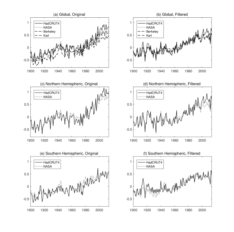
Figure 1: Global, Northern and Southern Hemispheric Temperature Series

The temperature series are affected by various modes of natural variability such as the Atlantic Multidecadal Oscillation (AMO) and the North Atlantic Oscillation (NAO), which are characterized by low frequency movements (Kerr, 2000; Hurrell, 1995). Since trends and breaks are low frequency features, it is important to purge them from the temperature series allowing more precise estimates of the break dates. Other high frequency fluctuations in temperature series do not affect the precision of the estimates of the break dates and the magnitudes of the changes in slope. Accordingly, we filter out the effect of these modes of variability by regressing each temperature series on these modes and a constant. Since the effect of natural variability might have occurred with a time lag, we choose an appropriate lag using the Bayesian Information Criterion (BIC); Schwarz (1978). The candidate regressors for the filtering are the current value and lags (up to order $kmax-1$) of AMO and NAO. We first work with G from HadCRUT4. We start with $kmax=2$, so that the candidates are the current value and the first lag only. BIC chooses the current value of AMO and the first lag of NAO. Since the maximum lag allowed is selected, we increase $kmax$ to 4. Then, BIC chooses the current value of AMO and the second lag of NAO (the first is not included given that we search over models not necessarily including all lags up to some chosen order). When applying the BIC, the number of observations used is limited by $kmax$ (e.g., Perron and Ng, 2005). Having decided on the current value of AMO and the second lag of NAO, we apply the filtering to all available observations, not limited by $kmax$. We could repeat the same procedure to each series. However, it does not make much sense to have the same mode affect each temperature series with a different lag. Hence, we filter all series with the current value of AMO and the second lag of NAO. The filtered temperature series are denoted as G̃, Ñ and S̃. Figure 1 presents graphs of the original and filtered series.

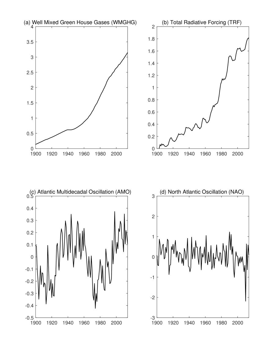
Figure 2: Radiative Forcing Variables and Modes of Variablility

For the radiative forcing variables, we use WMGHG and TRF. Figure 2 displays the time plots of WMGHG and TRF as well as the AMO and NAO. The data set used covers the period 1880-2014 and the filtering is done with the full sample. We use the data for 1900-2014 for the purpose of the common break date tests. We use two sample periods: 1900-1992 and 1963-2014. The reason we split the sample is to reduce the number of breaks in the system, thereby lessening the computational burden. Our choice of sample periods is made with the intention to minimize any unwanted effect from a second break that might exist in any of the variables in the system. The break dates in WMGHG are estimated most precisely since it has a very small noise component (see Figure 2) and they are 1963 and 1992. First we consider bivariate systems with one temperature series and one radiative forcing series. The null hypothesis of a common break date is tested using the LR test from Theorem 1. Since this test is not asymptotically pivotal, we supply bootstrap p-values as well. The bootstrap is carried out in the same way as done in the Monte Carlo simulations reported earlier. We also report the GLS-Wald test from Theorem 2. Although the GLS-Wald test is asymptotically pivotal, we still supply the bootstrap p-values because of the size distortions observed in our Monte Carlo study. In addition to the 4 global, 2 northern hemispheric and 2 southern hemispheric temperature series, we also consider the average of the global, northern and southern hemispheric temperature series across different datasets. Hence, there are 11 temperature series and 11 filtered temperature series, each of which is paired with either WMGHG or TRF, yielding a total of 44 bivariate systems.

Table 4 (a) reports the results for the sample period of 1900-1992 when the original temperature series are considered; the asymptotic p-values of the Wald and LR test are very small in most cases and the null of a common break date is rejected with only a few exceptions. However, the bootstrap p-values are well over the conventional thresholds 0.05 or 0.01 in all cases. Given the previous simulation results, we view the bootstrap p-values as more reliable than the asymptotic ones. Note that the break date for the radiative forcing variable is almost unchanged at either 1963 or 1966, regardless of the temperature series in the bivariate system. Also, the estimated common break date, i.e., the estimate imposing the null of common breaks, always coincide with the break date for the radiative forcing variable. On the other hand, the break date estimates for the temperature series are quite spread out. Hence, the break dates in the radiative forcing variables are being estimated more precisely than those in the temperature series. The large p-values produced by the bootstrapping is a consequence of the high level of noise in the temperature series relative to the magnitude of the break. Accordingly, we fail to reject the null of a common break date despite the large discrepancy in the estimated break dates. Table 4 (a) also shows the results obtained with the filtered temperature series. The picture changes quite dramatically. The break dates for the radiative forcing variables are still at 1963 or 1966, but those for the temperature series are now also around 1960. Especially, when TRF enters the bivariate system, the estimate of the break date is 1960, 1965 or 1966, the exception being the southern hemispheric temperature from HadCRUT4 and the average of the two southern hemispheric temperature series, for which the estimate is still 1956. As a result, both the asymptotic and bootstrap p-values are much larger than those for the original temperature series.

Tables 4 (b) presents the results for the second sample 1963-2014 when the original temperature series are used and the estimates of the break dates for the temperature series are again quite spread out, while those for the radiative forcing variables are consistently around 1990-1992. Just like in Table 4 (a), the asymptotic p-values suggest strong rejection of the null hypothesis, but the bootstrap p-values turns out much larger reflecting again the high level of correlated noise in the original series. Note that the estimates of the break dates for the filtered temperature series are 1990-1992 with only a few exceptions. Also, the p-values are larger than the corresponding ones for the original temperature series.

We repeat the analysis for the bivariate systems with the OLS-Wald test as a robustness check and report the results in Table 5. The results are very similar when the filtered series are considered. The break date estimates obtained equation by equation coincide with those obtained from the system or differ only by a few years at most. When the original series are used, the break date estimates for some series largely deviate from those computed by the system method. However, the fact that the bootstrap p-values are much larger than usual thresholds still applies. Thus, our conclusions remain the same.

An advantage of the OLS-Wald test is that it can handle a larger system without extra computational burden. The break date estimates will not change if we consider a larger system, because they are computed equation by equation. However, the long-run variance estimate and the bootstrap p-values can change as we consider a bigger system. We consider three five-variables systems. Each system has a global, northern and southern hemispheric temperature and the two radiative forcing variables. The first one uses the temperature series from HadCRUT4, the second one from NASA and the third one has average global, northern and southern hemispheric temperature series. The results are reported in Table 6. They show results broadly similar to those obtained bivariate systems.

To provide a final robustness check, we consider testing jointly whether the two breaks near 1960 and for the “hiatus” are common. We use the OLS-Wald test, which estimates the two breaks jointly for each equation, and the period 1926-2014 to focus on the time span whereby anthropogenic factors are most likely to be the main driver affecting changes in temperatures. The results are presented in Table 7. The results obtained are broadly similar and lead to the same conclusions. When using the filtered series and the bootstrap p-values, the test fails to reject the null hypothesis of two common breaks. The first is located in the early 60’s (the onset of sustained global warming) and the second in the early 90’s (the “hiatus”) consistent with methods dealing with one break at a time presented earlier.

6.3 Testing for the “hiatus”

The literature on the existence and drivers of the current slowdown in the rate of warming has expanded quickly (Tollefson, 2014, 2016). In this section, we focus on testing if the “hiatus” can be explained by natural variability or if it is a feature of the underlying warming trend (Estrada, Perron and Martinez, 2013). A small part of the literature investigating the slowdown in the warming in global temperatures are based on formal structural change/change-point tests (Cahill et al., 2015; Pretis et al., 2015), while others are simply based on testing for trends during arbitrarily selected periods of time (Cahill et al., 2015; Foster and Rahmstorf, 2011; Lewandowsky et al., 2015). This type of approach, as well as most of physical-based studies, have typically failed to find convincing evidence for the existence of a change in the slope of global temperatures during the last decades. According to one of the commonly accepted hypothesis, the apparent “hiatus” is produced by the effects of low-frequency natural variability that result from coupled ocean-atmosphere processes and heat exchange between the ocean and the atmosphere. It has been proposed that effects of natural variability modes such as AMO, NAO and PDO were able to mask the warming trend since the 1990s, creating the illusion of a slowdown in the underlying warming trend (e.g., Guan et al ., 2015; Steinman et al., 2015; Li, Sun and Jin, 2013; Trenberth and Fasullo, 2013). However, Estrada and Perron (2016) argue that low-frequency oscillations do distort the underlying warming trend but cannot account for the current slowdown. Instead, the main effect of these oscillations has been to make it more difficult to detect the drop in the rate of warming, a real feature of the warming trend imparted by the slowdown in the radiative forcing from well-mixed greenhouse gases.

Establishing whether the “hiatus” period is statistically significant is important because it would counter the widely held view that it is the product of natural internal variability (Kosaka and Xie, 2013; Trenberth and Fasullo, 2013; Meehl et al., 2011; Balmaseda, Trenberth and Källén, 2013). Using standard tests (e.g., Perron and Yabu, 2009), the results are mixed across various series and sometimes borderline. Our aim is to provide tests with enhanced power by casting the testing problem in a bivariate framework involving temperatures and radiative forcing. We consider bivariate systems with one temperature series and one forcing variable. We use the LR test for the presence of a break in temperature series given the presence of a structural break in radiative forcing series. We first estimate a break date in the radiative forcing series under the likelihood framework for a bivariate system of a pair of radiative forcing and temperature series. Then, given the estimated break date in the radiative forcing series, we apply the LR test for the null hypothesis of no break in temperatures versus one break. To obtain $p$-values, we apply the bootstrap procedure described in Section 5 with 1,000 samples. The results are presented in Table 8. First, as expected from previous results, the LR test is more likely to reject the null hypothesis of no break when using filtered temperature series. Hence, we report results only for that case. For the filtered series from 1900 to 1992, we reject the null at less than 5% significance level in all pairs of radiative forcing and temperature series. Hence, there is clear evidence of a break in temperatures that is near 1960 (varying between 1954 and 1966 depending on the series and the forcing). This concurs with the common break results obtained in the previous section. When using the sample 1963-2014 we reject the null in seven and eight cases out of eleven filtered series at the 10% significance level with well-mixed green-house gases and total radiating forcing, respectively. Since the sample size is small ($T=52)$, we might expect that the LR test may have little power, but our result suggests strong evidence for the presence of a break in temperature series. Note that the evidence for a break is stronger when using bivariate systems involving TRF. This is due to the fact that TRF exhibits a larger decrease in slope compared to WMGHG. The errors are also more strongly correlated. For instance, solar irradiance is a part of both TRF and temperatures and an important source of variations. When considering systems with TRF, the only pairs that do not allow a rejection at the 10% level are those associated with Northern hemisphere temperatures. For these, the p-values range from .14 to .19, while for all other pairs they are below 10%. Given that the small sample size is small, the overall evidence strongly indicates a break in temperatures in the early 90s consistent with the presence of the much-debated “hiatus”.

7 Conclusion

We consider a multivariate system with $n$ equations with the dependent variables modeled as joint-segmented trends with multiple changes in slope. The errors can be serially correlated and correlated across equations. We consider testing for general linear restrictions on the break dates, including testing for common breaks across equations. The test used is a (quasi-) likelihood ratio test assuming serially uncorrelated errors. Under the stated conditions, the LR test has a pivotal chi-square distribution, though it is non-pivotal in general cases of interest. Hence, we also consider a corrected Wald test having a pivotal limit distribution, which can be constructed using break dates estimated one equation at a time or via the complete system. The limit distribution of the test is standard chi-square. However, simulations show that the two Wald tests suffer from potentially severe liberal size distortions for moderate to strong serial correlation. Hence, for all three tests, we suggest a bootstrap procedure to obtain the relevant critical values. These bootstrap tests are shown to have correct size in all cases considered. Our empirical results show that, once we filter the temperature data for the effect of the Atlantic Mutidecadal Oscillation (AMO) and the North Atlantic Oscillation (NAO), the breaks in the slope of radiative forcing and temperatures are common, both for the large increase in the 60s and the recent “hiatus”.

We also consider a test for the presence of an additional break in some series. The theoretical framework is general and allows multiple breaks in a general multivariate system. The test considered is a quasi-likelihood ratio test. The limit distribution is shown to be non-pivotal and depends in a complex way on a number of nuisance parameters. Hence, we use a bootstrap procedure to obtain relevant critical values. In our applications, the null and alternative hypotheses specify a break in the slope of the radiative forcing series, while under the null hypothesis there is no break in the temperature series but there is one under the alternative hypothesis. Our results indicate that indeed the “hiatus” represents a significant slowdown in the rate of increase in temperatures, especially when considering global or southern hemisphere series, for which our test points to a rejection of the null of no change for all data sources considered. The statistical results are of independent interest and applicable more generally beyond the climate change applications considered.

Appendix

Proof of Theorems 1 and 2: Let $\hat{\lambda}_{r}=\arg\min_{\lambda\text{ s.t. }R\lambda=r}|\hat{\Sigma}(\lambda)|$ and $\hat{\lambda}=\min_{\lambda}|\hat{\Sigma}(\lambda)|$. Given the consistency of $\hat{\Sigma}(\hat{\lambda}_{r})$, $\hat{\Sigma}(\hat{\lambda})$ and $\hat{\Sigma}(\lambda^{0})$ under the null hypothesis, we can apply a Taylor series expansion to $LR$ such that

$$LR = T~{}tr[\hat{\Sigma}^{-1}(\hat{\lambda})(\hat{\Sigma}(\hat{\lambda}_{r})-\hat{\Sigma}(\hat{\lambda}))]+o_{p}(1)$$ (A.1)

$$= T~{}tr[\hat{\Sigma}^{-1}(\hat{\lambda})(\hat{\Sigma}(\hat{\lambda}_{r})-\hat{\Sigma}(\lambda^{0}))]-T~{}tr[\hat{\Sigma}^{-1}(\hat{\lambda})(\hat{\Sigma}(\hat{\lambda})-\hat{\Sigma}(\lambda^{0}))]+o_{p}(1).$$

Consider the first term in the above decomposition. We may write

$$T~{}tr[\hat{\Sigma}^{-1}(\hat{\lambda})\left(\hat{\Sigma}(\hat{\lambda}_{r})-\hat{\Sigma}(\lambda^{0})\right)]=tr[\hat{\Sigma}^{-1}(\hat{\lambda})(\hat{U}_{\hat{\lambda}_{r}}^{\prime}\hat{U}_{\hat{\lambda}_{r}}-\hat{U}_{\lambda^{0}}^{\prime}\hat{U}_{\lambda^{0}})]$$

$$=tr[\Sigma^{-1}(\widetilde{U}_{\hat{\lambda}_{r}}^{\prime}\widetilde{U}_{\hat{\lambda}_{r}}-\widetilde{U}_{\lambda^{0}}^{\prime}\widetilde{U}_{\lambda^{0}})]+o_{p}(1)=\min_{\lambda\text{ s.t. }R\lambda=r}tr[\Sigma^{-1}(\widetilde{U}_{\lambda}^{\prime}\widetilde{U}_{\lambda}-\widetilde{U}_{\lambda^{0}}^{\prime}\widetilde{U}_{\lambda^{0}})]+o_{p}(1),$$

where $\widetilde{U}_{\lambda}$ is the matrix of estimated residuals from the infeasible GLS estimator, instead of the ML estimator, for $\lambda$. For notational simplicity, write $\Omega=\Sigma\otimes I_{T}$ and $M(\lambda)=I-\Omega^{-1/2}X(X^{\prime}\Omega^{-1}X)^{-1}X^{\prime}\Omega^{-1/2}$. Then the test statistic admits the following decomposition:

$$tr[\Sigma^{-1}(\widetilde{U}_{\lambda}^{\prime}\widetilde{U}_{\lambda}-\widetilde{U}_{\lambda^{0}}^{\prime}\widetilde{U}_{\lambda^{0}})]=vec(\widetilde{U}_{\lambda})^{\prime}\Omega^{-1}vec(\widetilde{U}_{\lambda})-vec(\widetilde{U}_{\lambda^{0}})^{\prime}\Omega^{-1}vec(\widetilde{U}_{\lambda^{0}})$$

$$=\theta^{\prime}(X^{0}-X)^{\prime}\Omega^{-1/2\prime}M(\lambda)\Omega^{-1/2}(X^{0}-X)\theta+2\theta^{\prime}(X^{0}-X)^{\prime}\Omega^{-1/2\prime}M(\lambda)\Omega^{-1/2}u$$

$$+u^{\prime}\Omega^{-1/2\prime}\left[M(\lambda)-M(\lambda^{0})\right]\Omega^{-1/2}u$$

$$\equiv(XX)+2(XU)+(UU)\text{.}$$ (A.2)

Note that

$$\left[X(k_{i}^{0})-X(k_{i})\right]\theta_{i} = [0,0,b(k_{i1}^{0})-b(k_{i1}),\dots,b(k_{im_{i}}^{0})-b(k_{im_{i}})]\theta_{i}$$

$$= [0,0,(k_{i1}-k_{i1}^{0})\widetilde{\iota}(k_{i1}),\dots,(k_{im_{i}}-k_{im_{i}}^{0})\widetilde{\iota}(k_{im_{i}})]\theta_{i}$$

$$= [(k_{i1}-k_{i1}^{0})\widetilde{\iota}(k_{i1}),\dots,(k_{im_{i}}-k_{im_{i}}^{0})\widetilde{\iota}(k_{im_{i}})]\delta_{i}\equiv\widetilde{\iota}(k_{i})diag(\delta_{i})(k_{i}-k_{i}^{0}),$$

where $\delta_{i}=(\delta_{i1},\dots,\delta_{im_{i}})^{\prime}$, $\widetilde{\iota}(k_{ij})=(k_{ij}-k_{ij}^{0})^{-1}(b(k_{ij}^{0})-b(k_{ij}))$, $k_{i}=(k_{i1},\dots,k_{im_{i}})^{\prime}$ and $\widetilde{\iota}(k_{i})=[\widetilde{\iota}(k_{i1}),\dots,\widetilde{\iota}(k_{im_{i}})]$. Now,

$$\left[X^{0}-X\right]\theta = \begin{pmatrix}\left[X(k_{1}^{0})-X(k_{1})\right]\theta_{1}&&0\\ &\ddots&\\ 0&&\left[X(k_{n}^{0})-X(k_{n})\right]\theta_{n}\end{pmatrix}$$

$$= \begin{pmatrix}\widetilde{\iota}(k_{1})&&0\\ &\ddots&\\ 0&&\widetilde{\iota}(k_{n})\end{pmatrix}\begin{pmatrix}D_{\delta_{1}}&&0\\ &\ddots&\\ 0&&D_{\delta_{n}}\end{pmatrix}\begin{pmatrix}k_{1}-k_{1}^{0}\\ \vdots\\ k_{n}-k_{n}^{0}\end{pmatrix}\equiv\Psi(\delta)(k-k^{0}),$$

with $D_{\delta_{i}}=diag(\delta_{i})$. Thus

$$\left|(XX)\right| \leq \left\|\Omega^{-1/2}(X^{0}-X)\theta\right\|^{2}\leq\left\|\Omega^{-1/2}\right\|^{2}\left\|(X^{0}-X)\theta\right\|^{2}$$

$$= \left\|\Omega^{-1/2}\right\|^{2}\left\|\Psi(\delta)(k-k^{0})\right\|^{2}\leq\left\|\Omega^{-1/2}\right\|^{2}\left\|\Psi(\delta)\right\|^{2}\left\|k-k^{0}\right\|^{2}=O(T)\left\|k-k^{0}\right\|^{2},$$

where the last equality follows from Lemma 1 of Perron and Zhu (2005). In addition, the $O(T)$ term in the above equation is not $o(T)$ and $(XX)>0$.

$$\left|(XU)\right| = \left|\theta^{\prime}(X^{0}-X)^{\prime}\Omega^{-1/2\prime}M(\lambda)\Omega^{-1/2}u\right|=\left|(k-k^{0})^{\prime}\Psi(\delta)^{\prime}\Omega^{-1/2\prime}M(\lambda)\Omega^{-1/2}u\right|$$

$$\leq \left\|k-k^{0}\right\|\left\|\Psi(\delta)^{\prime}\Omega^{-1/2\prime}M(\lambda)\Omega^{-1/2}u\right\|=\left\|k-k^{0}\right\|O_{p}(T^{1/2}).$$

For $(UU)$, note that

$$(UU) = u^{\prime}\Omega^{-1/2\prime}\left[M(\lambda)-M(\lambda^{0})\right]\Omega^{-1/2}u$$

$$= u^{\prime}\Omega^{-1}X^{0}(X^{0\prime}\Omega^{-1}X^{0})^{-1}X^{0\prime}\Omega^{-1}u-u^{\prime}\Omega^{-1}X(X^{\prime}\Omega^{-1}X)^{-1}X^{\prime}\Omega^{-1}u$$

$$= u^{\prime}\Omega^{-1}(X^{0}-X)(X^{0\prime}\Omega^{-1}X^{0})^{-1}X^{0\prime}\Omega^{-1}u$$

$$+u^{\prime}\Omega^{-1}X(X^{\prime}\Omega^{-1}X)^{-1}\left(X^{\prime}\Omega^{-1}X-X^{0\prime}\Omega^{-1}X^{0}\right)(X^{0\prime}\Omega^{-1}X^{0})^{-1}X^{0\prime}\Omega^{-1}u$$

$$+u^{\prime}\Omega^{-1}X(X^{\prime}\Omega^{-1}X)^{-1}(X_{0}-X)^{\prime}\Omega^{-1}u$$

$$= \left\|k-k^{0}\right\|O_{p}(T^{-1})\text{.}$$

These orders of magnitude show that $(XX)$, which is strictly positive, is the dominant term in (A.2). When these terms are evaluated at $k=\hat{k}_{r}$, $(XX)$ is still the dominant term and it contradicts to the fact that $tr[\Sigma^{-1}(\widetilde{U}_{\hat{\lambda}_{r}}^{\prime}\widetilde{U}_{\hat{\lambda}_{r}}-\widetilde{U}_{\lambda^{0}}^{\prime}\widetilde{U}_{\lambda^{0}})]<0$. The only way to avoid the contradiction is to have $T^{1/2}||\hat{k}_{r}-k^{0}||=T^{3/2}(\hat{\lambda}_{r}-\lambda^{0})=O_{p}(1)$. Since the rate of convergence is obtained as $T^{3/2}$, the minimization can be carried out over the set

$$\Lambda_{T}=\{\lambda:|\lambda_{ij}-\lambda_{ij}^{0}|\leq MT^{-3/2}\text{ for all }i\text{, }j\text{ and some large constant }M\}\text{.}$$

On $\Lambda_{T}$, $(UU)$ is asymptotically negligible and can be ignored. Thus,

$$\min_{\lambda\text{ s.t. }R\lambda=r\text{ on }\Lambda_{T}}tr[\Sigma^{-1}(\widetilde{U}_{\lambda}^{\prime}\widetilde{U}_{\lambda}-\widetilde{U}_{\lambda^{0}}^{\prime}\widetilde{U}_{\lambda^{0}})]=\min_{\lambda\text{ s.t. }R\lambda=r\text{ on }\Lambda_{T}}(XX)+2(XU)+o_{p}(1)\text{.}$$

Defining $\varphi_{T}=T^{3/2}(\lambda-\lambda^{0})$ yields that

$$(XX)=\varphi_{T}^{\prime}\left[T^{-1}\Psi(\delta)^{\prime}\Omega^{-1/2}M(\lambda)\Omega^{-1/2}\Psi(\delta)\right]\varphi_{T},$$

and

$$(XU)=\varphi_{T}^{\prime}\left[T^{-1/2}\Psi(\delta)^{\prime}\Omega^{-1/2\prime}M(\lambda)\Omega^{-1/2}u\right]\text{.}$$

Define a $Tn\times m$ matrix $Z=T^{-1/2}M(\lambda^{0})\Omega^{-1/2}\Psi(\delta)$, a $Tn\times 1$ vector $z=M(\lambda^{0})\Omega^{-1/2}u$ and $Q=Z(Z^{\prime}Z)^{-1}R_{\perp}^{\prime}$ where the $(m-q)\times m$ matrix $R_{\perp}$ is such that $R(Z^{\prime}Z)^{-1}R_{\perp}^{\prime}=0$ for a $q\times m$ matrix of restrictions $R$. Then,

$$\min_{\lambda\text{ s.t. }R\lambda=r\text{ on }\Lambda_{T}}(XX)+2(XU) = \min_{\varphi_{T}\text{ s.t. }R\varphi_{T}=0\text{ on }\Lambda_{T}}\left[Z\varphi_{T}+z\right]^{\prime}\left[Z\varphi_{T}+z\right]-z^{\prime}z+o_{p}(1)$$

$$= z\left[I-Q(Q^{\prime}Q)^{-1}Q^{\prime}\right]z-z^{\prime}z+o_{p}(1)$$

$$= -z^{\prime}Q(Q^{\prime}Q)^{-1}Q^{\prime}z+o_{p}(1).$$

The second term in (A.1) is basically the same as the first except that there is no restriction on the break dates, so that $Q=Z$. It follows that

$$T~{}tr\left[\hat{\Sigma}^{-1}(\hat{\lambda})\left(\hat{\Sigma}(\hat{\lambda})-\hat{\Sigma}(\lambda^{0})\right)\right]=-z^{\prime}Z(Z^{\prime}Z)^{-1}Z^{\prime}z+o_{p}(1)\text{,}$$

and

$$LR = -z^{\prime}Q(Q^{\prime}Q)^{-1}Q^{\prime}z+z^{\prime}Z(Z^{\prime}Z)^{-1}Z^{\prime}z+o_{p}(1)$$

$$= z^{\prime}Z(Z^{\prime}Z)^{-1}R\left(R^{\prime}(Z^{\prime}Z)^{-1}R\right)^{-1}R^{\prime}(Z^{\prime}Z)^{-1}Z^{\prime}z+o_{p}(1)\text{.}$$

Note that

$$Z^{\prime}Z = \frac{1}{T}\Psi(\delta)^{\prime}\Omega^{-1/2\prime}M(\lambda^{0})\Omega^{-1/2}\Psi(\delta)$$

$$= \frac{1}{T}\Psi(\delta)^{\prime}\Omega^{-1}\Psi(\delta)-\frac{1}{T}\Psi(\delta)^{\prime}\Omega^{-1}X^{0}S_{T}\left(\frac{1}{T}S_{T}X^{0\prime}\Omega^{-1}X^{0}S_{T}\right)^{-1}\frac{1}{T}S_{T}X^{0\prime}\Omega^{-1}\Psi(\delta)$$

$$\rightarrow D_{\delta}\left[Q_{GG}-Q_{GF}Q_{FF}^{-1}Q_{FG}\right]D_{\delta}=\Xi_{1}\text{,}$$

where

$$S_{T}=diag\left\{\begin{bmatrix}1&&\\ &T^{-1}&\\ &&T^{-1}I_{m_{1}}\end{bmatrix},\dots,\begin{bmatrix}1&&\\ &T^{-1}&\\ &&T^{-1}I_{m_{n}}\end{bmatrix}\right\}\text{.}$$

For $Z^{\prime}z$, let $\epsilon=\Omega^{-1}u$, which means that $\epsilon_{t}=(\epsilon_{1t},...,\epsilon_{nt})^{\prime}=\Sigma^{-1}(u_{1t},...,u_{nt})^{\prime}$ and the partial sums of $\epsilon_{t}$ obeys a functional central limit theorem from Assumption 3, i.e., $T^{-1/2}\sum_{t=1}^{[Tr]}\epsilon_{t}\Rightarrow\bar{B}(r)=\Sigma^{-1}\Psi^{1/2}W(r)$. Denote the $i^{th}$ element of $\bar{B}(r)$ by $\bar{B}_{i}(r)$. We can then express the limit of $Z^{\prime}z$ as the follows:

$$Z^{\prime}z = T^{-1/2}\Psi(\delta)^{\prime}\Omega^{-1/2\prime}M(\lambda^{0})\Omega^{-1/2}u$$

$$= T^{-1/2}\Psi(\delta)^{\prime}\Omega^{-1}u-T^{-1}\Psi(\delta)^{\prime}\Omega^{-1}X^{0}S_{T}\left(T^{-1}S_{T}X^{0\prime}\Omega^{-1}X^{0}S_{T}\right)^{-1}T^{-1/2}S_{T}X^{0\prime}\Omega^{-1}u$$

$$= \begin{bmatrix}-T^{-1}\Psi(\delta)^{\prime}\Omega^{-1}X^{0}S_{T}\left(\frac{1}{T}S_{T}X^{0\prime}\Omega^{-1}X^{0}S_{T}\right)^{-1}&I\end{bmatrix}\begin{bmatrix}T^{-1/2}S_{T}X^{0\prime}\epsilon\\ T^{-1/2}\Psi(\delta)^{\prime}\epsilon\end{bmatrix}$$

$$\overset{d}{\rightarrow}\begin{bmatrix}-D_{\delta}Q_{GF}Q_{FF}^{-1}&I_{m}\end{bmatrix}\times$$

$$\left(\begin{array}[]{cccccc}\int f_{1}(r)^{\prime}d\bar{B}_{1}(r)&\cdots&\int f_{n}(r)^{\prime}d\bar{B}_{n}(r)&\int g_{1}(r)^{\prime}d\bar{B}_{1}(r)&\cdots&\int g_{n}(r)^{\prime}d\bar{B}_{n}(r)\end{array}\right)^{\prime},$$

where the covariance of the vector of stochastic integrals in the above expression is given by

$$\left(\begin{array}[]{cc}\Gamma_{FF}&\Gamma_{FG}D_{\delta}\\ D_{\delta}\Gamma_{GF}&D_{\delta}\Gamma_{GG}D_{\delta}\end{array}\right)\text{.}$$

Thus, $Z^{\prime}z\overset{d}{\rightarrow}N\left(0,\Xi_{0}\right)$. Theorem 1 assumes that $\Sigma=\Psi$, hence $\Xi_{0}=\Xi_{1}$. Then, it follows that $LR\overset{d}{\rightarrow}\chi_{q}^{2}$. For Theorem 2, $T^{3/2}(\hat{\lambda}-\lambda^{0})=\hat{\varphi}_{T}+o_{p}(1)=-(Z^{\prime}Z)^{-1}Z^{\prime}z\overset{d}{\rightarrow}N(0,\Xi_{1}^{-1}\Xi_{0}\Xi_{1}^{-1\prime})$.

Proof of Corollary 1: Similarly to (A.2), we have the following decomposition

$$SSR_{i}(\lambda_{i})-SSR_{i}(\lambda_{i}^{0}) = \theta_{i}^{\prime}(X(k_{i}^{0})-X(k_{i}))^{\prime}M_{\lambda_{i}}(X(k_{i}^{0})-X(k_{i}))\theta_{i}$$

$$+2\theta_{i}^{\prime}(X(k_{i}^{0})-X(k_{i}))^{\prime}M_{\lambda_{i}}u_{i}$$

$$+u_{i}^{\prime}(M_{\lambda_{i}}-M_{\lambda_{i}^{0}})u_{i}$$

$$\equiv (XX)_{i}+2(XU)_{i}+(UU)_{i}.$$

The results in Perron and Zhu (2005) directly applies and $\widetilde{\lambda}_{i}$ is consistent at rate $T^{3/2}$. Thus, we can again focus on $T^{-3/2}$ neighborhood of $\lambda_{i}^{0}$, say $\Lambda_{iT}$, and

$$\widetilde{\lambda}_{i}=\arg\min_{\lambda_{i}\in\Lambda_{iT}}SSR_{i}(\lambda_{i})-SSR_{i}(\lambda_{i}^{0})=\arg\min_{\lambda_{i}\in\Lambda_{iT}}(XX)_{i}+2(XU)_{i}+o_{p}(1)\text{.}$$

Define $\varphi_{i}=T^{3/2}(\lambda_{i}-\lambda_{i}^{0})$ and $\Psi_{i}(\delta_{i})=\widetilde{\iota}(k_{i})D_{\delta_{i}}$. It follows that

$$T^{3/2}(\widetilde{\lambda}_{i}-\lambda_{i}^{0}) = \arg\min_{\varphi_{i}\in\Lambda_{iT}}\varphi_{i}^{\prime}\left[T^{-1}\Psi_{i}(\delta_{i})^{\prime}M_{\lambda_{i}}\Psi_{i}(\delta_{i})\right]\varphi_{i}+2\varphi_{i}^{\prime}\left[T^{-1/2}\Psi_{i}(\delta_{i})^{\prime}M_{\lambda_{i}}u_{i}\right]+o_{p}(1)$$

$$= -\left[T^{-1}\Psi_{i}(\delta_{i})^{\prime}M_{\lambda_{i}^{0}}\Psi_{i}(\delta_{i})\right]^{-1}\left[T^{-1/2}\Psi_{i}(\delta_{i})^{\prime}M_{\lambda_{i}^{0}}u_{i}\right]+o_{p}(1)\text{.}$$

Note that

$$T^{-1}\Psi_{i}(\delta_{i})^{\prime}M_{\lambda_{i}^{0}}\Psi_{i}(\delta_{i})\rightarrow D_{\delta_{i}}\left[\int p_{i}(r)p_{i}^{\prime}(r)dr\right]D_{\delta_{i}}$$

and

$$T^{-1/2}\Psi_{i}(\delta_{i})^{\prime}M_{\lambda_{i}^{0}}u_{i}\Rightarrow D_{\delta_{i}}\left[\int p_{i}(r)dB_{i}(r)\right],$$

where $B_{i}(r)$ is the $i^{th}$ element of $B(r)=\Psi^{1/2}W(r)$ in Assumption 3. Furthermore, the weak convergence holds jointly in $i$ under Assumption 3. Therefore,

$$T^{3/2}\begin{pmatrix}\widetilde{\lambda}_{1}-\lambda_{1}^{0}\\ \vdots\\ \widetilde{\lambda}_{n}-\lambda_{n}^{0}\end{pmatrix}\overset{d}{\rightarrow}N\left(0,\begin{pmatrix}\psi_{11}D_{\delta_{1}}^{-1}P_{11}D_{\delta_{1}}^{-1}&\dots&\psi_{1n}D_{\delta_{1}}^{-1}P_{1n}D_{\delta_{n}}^{-1}\\ \vdots&\ddots&\vdots\\ \psi_{n1}D_{\delta_{n}}^{-1}P_{n1}D_{\delta_{1}}^{-1}&\dots&\psi_{nn}D_{\delta_{n}}^{-1}P_{nn}D_{\delta_{n}}^{-1}\end{pmatrix}\right),$$

where $P_{ij}=(\int p_{i}(r)p_{i}^{\prime}(r)dr)^{-1}\int p_{i}(r)p_{j}^{\prime}(r)dr(\int p_{j}(r)p_{j}^{\prime}(r)dr)^{-1}$.

Proof of Theorem 3: We use $\hat{\Sigma}_{(i)}(k,h)$ and $\hat{\Sigma}_{(i)}(\lambda,\nu)$ interchangeably. As in (A.1),

$$LR=T~{}tr\left[\hat{\Sigma}_{(i)}^{-1}(\hat{\lambda},\hat{\nu})\left(\hat{\Sigma}(\hat{\lambda})-\hat{\Sigma}_{(i)}(\hat{\lambda},\hat{\nu})\right)\right]+o_{p}(1)\text{,}$$

where $\hat{\nu}=\arg\min_{\nu\in C_{T}^{(i)}}\log\left|\hat{\Sigma}_{(i)}(\hat{\lambda},\nu)\right|$. Define the projection matrix $P_{(i)}(\lambda,\nu)$ as

$$P_{(i)}(\lambda,\nu)=M(\lambda)\Omega^{-1/2}a_{i}\left(a_{i}^{\prime}\Omega^{-1/2\prime}M(\lambda)\Omega^{-1/2}a_{i}\right)^{-1}a_{i}^{\prime}\Omega^{-1/2\prime}M(\lambda)\text{,}$$

where $a_{i}=a_{i}([T\nu])$ for simplicity and $M(\lambda)=I-\Omega^{-1/2}X(X^{\prime}\Omega^{-1}X)^{-1}X^{\prime}\Omega^{-1/2}$. Then, it follows that

$$LR=\sup\nolimits_{\nu\in C_{T}^{(i)}}y^{\prime}\Omega^{-1/2\prime}M(\hat{\lambda})P_{(i)}(\hat{\lambda},\nu)M(\hat{\lambda})\Omega^{-1/2}y+o_{p}(1)\text{.}$$

Since

$$M(\lambda)\Omega^{-1/2}y = M(\lambda)\Omega^{-1/2}(X^{0}-X)\theta+M(\lambda)\Omega^{-1/2}u$$

$$= M(\lambda)\Omega^{-1/2}\Psi(\delta)(k-k^{0})+M(\lambda)\Omega^{-1/2}u,$$

we can write

$$LR=\sup_{\nu\in C_{T}^{(i)}}\left[\begin{array}[]{c}(\hat{k}-k^{0})^{\prime}\Psi(\delta)^{\prime}\Omega^{-1/2\prime}M(\hat{\lambda})P_{(i)}(\hat{\lambda},\nu)M(\hat{\lambda})\Omega^{-1/2}\Psi(\delta)(\hat{k}-k^{0})\\ +2(\hat{k}-k^{0})^{\prime}\Psi(\delta)^{\prime}\Omega^{-1/2\prime}M(\hat{\lambda})P_{(i)}(\hat{\lambda},\nu)M(\hat{\lambda})\Omega^{-1/2}u\\ +u^{\prime}\Omega^{-1/2\prime}M(\hat{\lambda})P_{(i)}(\hat{\lambda},\nu)M(\hat{\lambda})\Omega^{-1/2}u\end{array}\right]+o_{p}(1)\text{.}$$

From the proof of Theorem 1, recall that $\sqrt{T}(\hat{k}-k^{0})=-(Z^{\prime}Z)^{-1}Z^{\prime}z+o_{p}(1)$ where $Z=T^{-1/2}M(\lambda^{0})\Omega^{-1/2}\Psi(\delta)$ and $z=M(\lambda^{0})\Omega^{-1/2}u$. Then,

$$LR=\sup\nolimits_{\nu\in C^{(i)}}\left[\begin{array}[]{c}z^{\prime}\left(I-Z(Z^{\prime}Z)^{-1}Z^{\prime}\right)P_{(i)}(\lambda^{0},\nu)\left(I-Z(Z^{\prime}Z)^{-1}Z^{\prime}\right)z\end{array}\right]+o_{p}(1)\text{.}$$

To further analyze this expression, we write

$$z^{\prime}\left(I-Z(Z^{\prime}Z)^{-1}Z^{\prime}\right)P_{(i)}(\lambda^{0},\nu)\left(I-Z(Z^{\prime}Z)^{-1}Z^{\prime}\right)z$$

$$= \frac{(T^{-3/2}a_{i}^{\prime}\Omega^{-1/2\prime}M(\lambda^{0})\left(I-Z(Z^{\prime}Z)^{-1}Z^{\prime}\right)z)^{2}}{T^{-3}a_{i}^{\prime}\Omega^{-1/2\prime}M(\lambda^{0})\Omega^{-1/2}a_{i}}.$$

The weak convergence result for the numerator of (Inference Related to Common Breaks in a Multivariate System with Joined Segmented Trends with Applications to Global and Hemispheric Temperatures) follows from Assumption 3 and the continuous mapping theorem. To see this, consider the following decomposition.

$$T^{-3/2}a_{i}^{\prime}\Omega^{-1/2\prime}M(\lambda^{0})\left(I-Z(Z^{\prime}Z)^{-1}Z^{\prime}\right)z=A_{1}(\nu)A_{2}(\nu)A_{3}(\nu)\text{, say,}$$

with

$$A_{1}(\nu) = \left(1,-\left(T^{-3/2}a_{i}^{\prime}\Omega^{-1/2\prime}M(\lambda^{0})Z\right)(Z^{\prime}Z)^{-1}\right)$$

$$A_{2}(\nu) = \left(\begin{array}[]{ccc}1&-T^{-2}a_{i}^{\prime}\Omega^{-1}X^{0}S_{T}\left(\frac{1}{T}S_{T}X^{0\prime}\Omega^{-1}X^{0}S_{T}\right)^{-1}&0\\ 0&-T^{-1}\Psi(\delta)^{\prime}\Omega^{-1}X^{0}S_{T}\left(\frac{1}{T}S_{T}X^{0\prime}\Omega^{-1}X^{0}S_{T}\right)^{-1}&I_{m}\end{array}\right)$$

$$A_{3}(\nu) = \left(\begin{array}[]{ccc}T^{-3/2}a_{i}&T^{-1/2}(S_{T}X^{0\prime})&T^{-1/2}\Psi(\delta)\end{array}\right)^{\prime}\Omega^{-1}u\text{.}$$

For $A_{1}$, note that $Z^{\prime}Z\overset{p}{\rightarrow}\Xi_{1}$ from the proof of Theorem 1 and

$$T^{-3/2}a_{i}^{\prime}\Omega^{-1/2\prime}M(\lambda^{0})Z = T^{-2}a_{i}^{\prime}\Omega^{-1/2\prime}M(\lambda^{0})\Omega^{-1/2}\Psi(\delta)$$

$$= T^{-2}a_{i}^{\prime}\Omega^{-1}\Psi(\delta)$$

$$-T^{-2}a_{i}^{\prime}\Omega^{-1}X^{0}S_{T}\left(\frac{1}{T}S_{T}X^{0\prime}\Omega^{-1}X^{0}S_{T}\right)^{-1}T^{-1}S_{T}X^{0\prime}\Omega^{-1}\Psi(\delta)$$

$$\rightarrow [Q_{BG}^{(i)}(\nu)-Q_{BF}^{(i)}(\nu)Q_{FF}^{-1}Q_{FG}]D_{\delta}\text{,}$$

uniformly in $\nu$. Thus,

$$A_{1}(\nu)\rightarrow\left(1,-[Q_{BG}^{(i)}(\nu)-Q_{BF}^{(i)}(\nu)Q_{FF}^{-1}Q_{FG}]D_{\delta}\Xi_{1}^{-1}\right)=\left(1,-\varsigma_{1}^{\prime}(\nu)\Xi_{1}^{-1}\right)\text{,}$$ (A.7)

uniformly in $\nu$. Similarly, $A_{2}$ is such that

$$A_{2}(\nu)\rightarrow\left(\begin{array}[]{ccc}1&-Q_{BF}^{(i)}(\nu)Q_{FF}^{-1}&0\\ 0&-D_{\delta}Q_{GF}Q_{FF}^{-1}&I_{m}\end{array}\right)\text{,}$$ (A.8)

uniformly in $\nu$. For $A_{3}$, let $\bar{B}_{i}(r)$ be as defined in the proof of Theorem 1. Then,

$$A_{3}(\nu)=\left(\begin{array}[]{c}T^{-3/2}a_{i}^{\prime}\epsilon\\ T^{-1/2}S_{T}X^{0\prime}\epsilon\\ T^{-1/2}\Psi(\delta)^{\prime}\epsilon\end{array}\right)\Rightarrow\left(\begin{array}[]{ccc}1&&0\\ &I_{m+2n}&\\ 0&&D_{\delta}\end{array}\right)\left(\begin{array}[]{c}\int b(r,\nu)d\bar{B}_{i}(r)\\ \int f_{1}(r)d\bar{B}_{1}(r)\\ \vdots\\ \int f_{n}(r)d\bar{B}_{n}(r)\\ \int g_{1}(r)d\bar{B}_{1}(r)\\ \vdots\\ \int g_{n}(r)d\bar{B}_{n}(r)\end{array}\right),$$ (A.9)

over $\nu\in(0,1)$. Thus, $A_{3}$ is a Gaussian process with covariance matrix given by

$$\left(\begin{array}[]{ccc}\Gamma_{BB}^{(i)}(\nu)&\Gamma_{BF}^{(i)}(\nu)&\Gamma_{BG}^{(i)}(\nu)D_{\delta}\\ \Gamma_{FB}^{(i)}(\nu)&\Gamma_{FF}&\Gamma_{FG}D_{\delta}\\ D_{\delta}\Gamma_{GB}^{(i)}(\nu)&D_{\delta}\Gamma_{GF}&D_{\delta}\Gamma_{GG}D_{\delta}\end{array}\right)\text{.}$$

Therefore, combining (A.7), (A.8) and (A.9) yields the weak convergence result

$$T^{-3/2}a_{i}^{\prime}\Omega^{-1/2\prime}M(\lambda^{0})[I-Z(Z^{\prime}Z)^{-1}Z^{\prime}]z\Rightarrow\eta_{(i)}(\nu),$$ (A.10)

over $\nu\in(0,1)$. Lastly, the denominator in (Inference Related to Common Breaks in a Multivariate System with Joined Segmented Trends with Applications to Global and Hemispheric Temperatures) is such that

$$T^{-3}a_{i}^{\prime}\Omega^{-1/2\prime}M(\lambda^{0})\Omega^{-1/2}a_{i}$$

$$= T^{-3}a_{i}^{\prime}\Omega^{-1}a_{i}-T^{-2}a_{i}^{\prime}\Omega^{-1}X^{0}S_{T}\left(T^{-1}S_{T}X^{0\prime}\Omega^{-1}X^{0}S_{T}\right)^{-1}T^{-2}S_{T}X^{0\prime}\Omega^{-1}a_{i}$$

$$\rightarrow Q_{BB}^{(i)}(\nu)-Q_{BF}^{(i)}(\nu)Q_{FF}^{-1}Q_{FB}^{(i)}(\nu)=\xi_{1}^{(i)}(\nu)\text{,}$$

uniformly in $\nu$. The result in part (i) of the theorem follows from (A.10) and (Inference Related to Common Breaks in a Multivariate System with Joined Segmented Trends with Applications to Global and Hemispheric Temperatures). The result in part (ii) also follows since the above result holds jointly in $i$.

References

- 1 Andrews, D.W.K., 1991. Heteroskedasticity and autocorrelation consistent covariance matrix estimation. Econometrica 59, 817-858.
- 2 Bai, J., Perron, P., 1998. Estimating and testing linear models with multiple strucutral changes. Econometrica 66, 47-78.
- 3 Bai, J., Perron, P., 2003. Computation and analysis of multiple structural change models. Journal of Applied Econometrics 18, 1-22.
- 4 Balmaseda, M.A., Trenberth, K.E., Källén, E., 2013. Distinctive climate signals in reanalysis of global ocean heat content. Geophysical Research Letters 40, 1754-1759.
- 5 Bierens, H.J., 2000. Nonparametric Nonlinear Cotrending Analysis, with an application to interest and inflation in the United States. Journal of Business and Economic Statistics 18, 323–337.
- 6 Cahill, N., Rahmstorf, S., Parnell, A.C., 2015. Change points of global temperature. Environmental Research Letters 10(8), 084002.
- 7 Dickey. D.A., Fuller, W.A., 1979. Distribution of the estimators for autoregressive time series with a unit root. Journal of the American Statistical Association 74, 427–431.
- 8 Engle, R.F., Granger, C.W.J., 1987. Co-integration and error correction: representation, estimation and testing. Econometrica 55, 251-276.
- 9 Estrada, F., Perron, P., 2014. Detection and attribution of climate change through econometric methods. Boletín de la Sociedad Matemática Mexicana 20, 107-136.
- 10 Estrada, F., Perron, P., 2016. Extracting and analyzing the warming trend in global and hemispheric temperatures. Unpublished Manuscript, Department of Economics, Boston University.
- 11 Estrada, F., Perron, P., Gay-García, C., Martínez-López, B., 2013. A time-series analysis of the 20th century climate simulations produced for the IPCC’s Fourth Assessment Report. Plos One 8(3): e60017.
- 12 Estrada F., Perron P., Martínez-López B., 2013. Statistically derived contributions of diverse human influences to twentieth-century temperature changes. Nature Geoscience 6, 1050-1055.
- 13 Foster, G., Rahmstorf, S., 2011. Global temperature evolution 1979–2010. Environmental Research Letters 6(4), 044022.
- 14 Fyfe, J.C., Meehl, G.A., England, M.H., Mann, M.E., Santer, B.D., Flato, G.M., Hawkins, E., Gillett, N.P., Xie, S.P., Kosaka, Y., Swart, N.C., 2016. Making sense of the early-2000s warming slowdown. Nature Climate Change 6, 224–228.
- 15 Gallagher, C., Lund, R., Robbins, M., Gallagher, C., Lund, R., Robbins, M., 2013. Changepoint Detection in Climate Time Series with Long-Term Trends. Journal of Climate 26, 4994–5006.
- 16 Gay-Garcia, C., Estrada, F., Sanchez, A. 2009. Global and hemispheric temperature revisited. Climatic Change 94, 333-349.
- 17 Giacomini, R., Politis, D.N., White, H., 2013. A warp-speed method for conducting Monte Carlo experiments involving bootstrap estimators. Econometric Theory 29, 567-589.
- 18 GISTEMP Team, 2015. GISS surface temperature analysis (GISTEMP). NASA Goddard Institute for Space Studies. Dataset accessed at http://data.giss.nasa.gov/gistemp/
- 19 Guan, X., Huang, J., Guo, R., Pu, L., 2015. The role of dynamically induced variability in the recent warming trend slowdown over the Northern Hemisphere. Scientific Reports 5, 12669.
- 20 Hansen, J., Ruedy, R., Sato, M., Lo, K., 2010. Global surface temperature change. Reviews of Geophysics 48.4.
- 21 Hansen, J., Sato, M., Kharecha, P., von Schuckmann, K., 2011. Earths energy imbalance and implications. Atmospheric Chemistry and Physics 11, 13421-13449.
- 22 Harvey, D.I., Mills, T.C., 2002. Unit roots and double smooth transitions. Journal of Applied Statistics 29, 675–683.
- 23 Hurrell, J.W., 1995. Decadal trends in the North Atlantic Oscillation and relationships to regional temperature and precipitation. Science 269, 676-679.
- 24 Johansen, S., 1991. Estimation and hypothesis testing of cointegration vectors in Gaussian vector autoregressive models. Econometrica 59, 1551-1580.
- 25 Karl, T.R., Knight, R.W., Baker, B., 2000. The record breaking global temperatures of 1997 and 1998: Evidence for an increase in the rate of global warming? Geophysical Research Letters 27, 719–722.
- 26 Karl, T.R., Arguez, A., Huang, B., Lawrimore, J.H., McMahon, J.R., Menne, M.J., Peterson, T.C., Vose, R.S., Zhang, H.M., 2015 Possible artifacts of data biases in the recent global surface warming hiatus. Science 348, 1469–1472.
- 27 Kaufmann, R.K., Kauppi, H., Stock, J.H., 2006. Emissions, concentrations, & temperature: A time series analysis. Climatic Change 77, 249-278.
- 28 Kerr, R.A., 2000. A North Atlantic climate pacemaker for the centuries. Science 288, 1984-1985.
- 29 Kilian, L., 1998. Small-sample confidence intervals for impulse response functions. Review of Economics and Statistics 80, 218-230.
- 30 Kim, D., Perron, P., 2009. Unit root tests allowing for a break in the trend function at an unknown time under both the null and alternative hypotheses. Journal of Econometrics 148, 1-13.
- 31 Kosaka. Y., Xie, S.P., 2013. Recent global-warming hiatus tied to equatorial Pacific surface cooling. Nature 501, 403–407.
- 32 Lewandowsky, S., Risbey, J.S., Oreskes, N., 2015. On the definition and identifiability of the alleged “hiatus” in global warming. Scientific Reports 5:16784.
- 33 Lewandowsky, S., Risbey, J.S., Oreskes, N., 2016. The pause in global warming: Turning a routine fluctuation into a problem for science. Bulletin of the American Meteorological Society 97, 723-733.
- 34 Li, J., Sun, C., Jin, F.F., 2013. NAO implicated as a predictor of Northern Hemisphere mean temperature multidecadal variability. Geophysical Research Letters 40, 5497-5502.
- 35 Mantua, N.J., Hare, S.R., 2002. The Pacific Decadal Oscillation. Journal of Oceanography 58.1, 35-44.
- 36 Meehl, G.A., Arblaster, J.M., Fasullo, J.T., Hu, A., Trenberth, K.E., 2011. Model-based evidence of deep-ocean heat uptake during surface-temperature hiatus periods. Nature Climate Change 1, 360–364.
- 37 Mills, T.C., 2013. Breaks and unit roots in global and hemispheric temperatures: An updated analysis. Climatic Change 118, 745–755.
- 38 Morice, C.P., Kennedy, J.J., Rayner, N.A., Jones, P.D., 2012. Quantifying uncertainties in global and regional temperature change using an ensemble of observational estimates: The HadCRUT4 dataset. Journal of Geophysical Research 117, D8.
- 39 Ng, S., Perron, P., 2001. Lag length selection and the construction of unit root tests with good size and power. Econometrica 69, 1519-1554.
- 40 Oka, T., Perron, P., 2016. Testing for common breaks in a multiple equation system. Unpublished Manuscript, Department of Economics, Boston University.
- 41 Perron, P., 1989. The great crash, the oil price shock, and the unit root hypothesis. Econometrica 57, 1361-1401.
- 42 Perron, P., 1997. Further evidence on breaking trend functions in macroeconomic variables. Journal of Econometrics 80, 355-385.
- 43 Perron, P., Ng, S., 2005. A note on the selection of time series models. Oxford Bulletin of Economics and Statistics 67, 115-134.
- 44 Perron, P., Zhu, X., 2005. Structural breaks with deterministic and stochastic trends. Journal of Econometrics 129, 65-119.
- 45 Perron P, Yabu T., 2009. Testing for shifts in trend with an integrated or stationary noise component. Journal of Business & Economic Statistics 27, 369-396.
- 46 Pretis, F., Mann, M.L., Kaufmann, R.K., 2015. Testing competing models of the temperature hiatus: assessing the effects of conditioning variables and temporal uncertainties through sample-wide break detection. Climatic Change 131, 705–718.
- 47 Qu, Z., Perron, P., 2007. Estimating and testing structural changes in multivariate regressions. Econometrica 75, 459-502.
- 48 Reeves, J., Chen, J., Wang, X.L., Lund, R., Lu, Q.Q., Reeves, J., Chen, J., Wang, X.L., Lund, R., Lu, Q.Q., 2007. A Review and Comparison of Changepoint Detection Techniques for Climate Data. Journal of Applied Meteorology and Climatology 46, 900–915.
- 49 Rohde, R., Muller, R., Jacobsen, R., Perlmutter, S., Rosenfeld, A., Wurtele, J., Curry, J., Wickhams, C. and Mosher, S., 2013. Berkeley Earth Temperature Averaging Process, Geoinformatics and Geostatistics: An Overview 1(2), 20-100.
- 50 Schwarz, G.E., 1978. Estimating the dimension of a model. Annals of Statistics 6, 461–464.
- 51 Seidel, D.J., Lanzante, J.R., 2004. An assessment of three alternatives to linear trends for characterizing global atmospheric temperature changes. Journal of Geophysical Research: Atmospheres 109, D14.
- 52 Steinman, B.A., Mann, M.E., Miller, S.K., 2015. Atlantic and pacific multidecadal oscillations and northern hemisphere temperatures. Science 347, 988–991.
- 53 Stocker, T.F., Qin, D., Plattner, G.K., Tignor, M., Allen, S.K., Boschung, J., Nauels, A., Xia, Y., Bex, B., Midgley, B.M., 2013. IPCC, 2013: climate change 2013: The physical science basis. Contribution of Working roup I to the Fifth Assessment Report of the Intergovernmental Panel on Climate Change.
- 54 Swanson, K.L., Sugihara, G., Tsonis, A.A., 2009. Long-term natural variability and 20th century climate change. Proceedings of the National Academy of Sciences 106.38, 16120-16123.
- 55 Tol, R.S.J., De Vos, A.F. 1993 Greenhouse statistics - time series analysis. Theoretical and Applied Climatology, 48, 63–74.
- 56 Tol, R.S.J., De Vos, A.F. 1998. A Bayesian statistical analysis of the enhanced greenhouse effect. Climatic Change 38, 87-112.
- 57 Tollefson, J., 2014. Climate change: The case of the missing heat. Nature 505, 276–278.
- 58 Tollefson, J., 2016. Global warming “hiatus” debate flares up again. Nature. doi:10.1038/nature.2016.19414.
- 59 Tomé, A.R., Miranda, P.M.A., 2004. Piecewise linear fitting and trend changing points of climate parameters. Geophysical Research Letters 31(2).
- 60 Trenberth, K.E., Fasullo, J.T., 2013. An apparent hiatus in global warming? Earth’s Future 1, 19–32.
- 61 Wolter, K., Timlin, M.S., 1998. Measuring the strength of ENSO events: how does 1997/98 rank?. Weather 53, 315-324.
- 62 Wu, Z., Huang, N.E., Wallace, J.M., Smoliak, B. V., Chen, X., 2011. On the time-varying trend in global-mean surface temperature. Climate Dynamics 37, 759–773.