A Light Curve Analysis of Recurrent and Very Fast Novae
in our Galaxy, Magellanic Clouds, and M31

Abstract

We analyzed optical, UV, and X-ray light curves of 14 recurrent and very fast novae in our galaxy, Magellanic Clouds, and M31, and obtained their distances and white dwarf (WD) masses. Among the 14 novae, we found that eight novae host very massive ($\gtrsim 1.35~{}M_{\sun}$) WDs and are candidates of Type Ia supernova (SN Ia) progenitors. We confirmed that the same timescaling law and time-stretching method as in galactic novae can be applied to extra-galactic fast novae. We classify the four novae, V745 Sco, T CrB, V838 Her, and V1534 Sco, as the V745 Sco type (rapid-decline), the two novae, RS Oph and V407 Cyg, as the RS Oph type (circumstellar matter(CSM)-shock), and the two novae, U Sco and CI Aql, as the U Sco type (normal-decline). The $V$ light curves of these novae almost overlap with each other in the same group, if we properly stretch in the time direction (timescaling law). We apply our classification method to LMC, SMC, and M31 novae. YY Dor, LMCN 2009a, and SMCN 2016 belong to the normal-decline type, LMCN 2013 to the CSM-shock type, and LMCN 2012a and M31N 2008-12a to the rapid-decline type. We obtained the distance of SMCN 2016 to be $d=20\pm 2$ kpc, suggesting that SMCN 2016 is a member of our galaxy. The rapid-decline type novae have very massive WDs of $M_{\rm WD}=1.37-1.385~{}M_{\sun}$ and are promising candidates of SN Ia progenitors. This type of novae are much fainter than the MMRD relations.

1 Introduction

Type Ia supernovae (SNe Ia) play a crucial role in astrophysics, because they are used as standard candles to measure cosmic distances (Perlmutter et al., 1999; Riess et al., 1998), and produce a major proportion of iron group elements in the chemical evolution of galaxies (Kobayashi et al., 1998). However, the progenitor systems have not yet been identified observationally or theoretically (see, e.g., Maoz et al., 2014, for a review). One of the promising evolutionary paths to SNe Ia is the single-degenerate (SD) scenario, in which a white dwarf (WD) accretes matter from a nondegenerate companion, grows in mass to near the Chandrasekhar mass, and explodes as a SN Ia triggered by central carbon burning (e.g., Nomoto, 1982; Hachisu et al., 1999a). The WD mass approaches the Chandrasekhar mass just before a SN Ia explosion. One of the candidates for such SD systems is a recurrent nova, because their optical light curves quickly decay and their supersoft X-ray source (SSS) phases are very short compared with other classical novae (e.g., Hachisu & Kato, 2001b; Hachisu et al., 2007; Ness et al., 2007; Schwarz et al., 2011; Pagnotta & Schaefer, 2014). The nova theory suggests that such very fast evolving novae harbor a very massive WD close to the Chandrasekhar mass (Hachisu & Kato, 2006, 2010; Kato et al., 2014). In the present paper, we analyze optical, near-infrared (NIR), ultra-violet (UV), and supersoft X-ray light curves of recurrent novae as well as very fast novae, and estimate their basic properties including the WD masses to study the possibility of SN Ia progenitors.

A classical nova is a thermonuclear runaway event in a mass-accreting WD in a binary. A recurrent nova is a classical nova with multiple recorded outbursts. Hydrogen ignites to trigger an outburst after a critical amount of hydrogen-rich matter is accreted on the WD. The photospheric radius of the hydrogen-rich envelope expands to red-giant (RG) size and the binary becomes bright in the optical range (e.g., Starrfield et al., 1972; Prialnik, 1986; Nariai et al., 1980). The hydrogen-rich envelope then emits strong winds (e.g., Kato & Hachisu, 1994; Hachisu & Kato, 2006). After the maximum expansion of the pseudo-photosphere, it begins to shrink, and the nova optical emission declines. Subsequently, UV emission dominates the spectrum and finally, supersoft X-ray emission increases. The nova outburst ends when the hydrogen shell burning ends. Various timescaling laws have been proposed to identify a common pattern among the nova optical light curves (see, e.g., introduction of Hachisu et al., 2008b).

Hachisu & Kato (2006) found that the optical and NIR light curves of several novae follow a similar decline law. Moreover, they found that the time-normalized light curves are independent of the WD mass, chemical composition of the ejecta, and wavelength. They called this property “the universal decline law.” The universal decline law was examined first in several well-observed novae and later in many other novae ($\gtrsim 30$ novae) (Hachisu & Kato, 2007, 2009, 2010, 2015, 2016a, 2016b; Hachisu et al., 2006b, 2007, 2008b; Kato et al., 2009; Kato & Hachisu, 2012). Hachisu & Kato (2006) defined a unique timescaling factor of $f_{\rm s}$ for optical, UV, and supersoft X-ray light curves of a nova. The shortest timescales (smallest $f_{\rm s}$) correspond to the WD masses in the range $1.37-1.38~{}M_{\sun}$. Therefore, the shortest $f_{\rm s}$ systems are candidates for immediate progenitors of SNe Ia (e.g., Hachisu & Kato, 2001b, 2010, 2016a, 2016b).

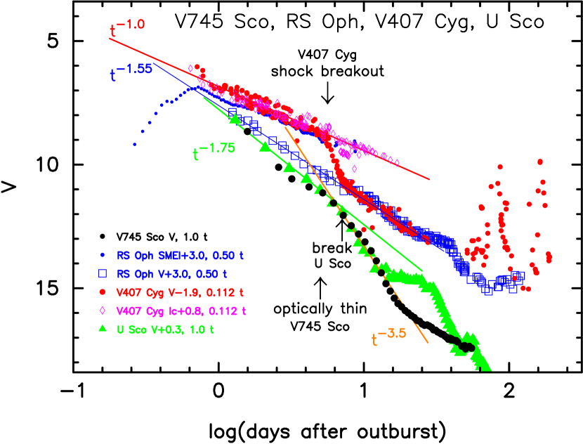
Figure 1: Three template $V$ light curves of the V745 Sco, RS Oph, and U Sco type novae. We add the $V$ and $I_{\rm C}$ light curves of V407 Cyg and the Solar Mass Ejection Imager (SMEI) magnitudes (Hounsell et al., 2010) of RS Oph for comparison. Each light curve is horizontally moved by $\Delta\log t=\log f_{\rm s}$ and vertically shifted by $\Delta V$ with respect to that of V745 Sco, as indicated in the figure by, for example, “RS Oph V+3.0, 0.50 t,” where $\Delta V=3.0$ and $f_{\rm s}=0.50$. The data are the same as those in Figures 3, 21, and 23. The filled black circles represent the $V$ light curve of the V745 Sco (2014) outburst. The filled red circles and open magenta diamonds denote the $V$ and $I_{\rm C}$ magnitudes of V407 Cyg, respectively. The blue dots and open blue squares denote the SMEI and $V$ magnitudes of the RS Oph (2006) outburst, respectively. The filled green triangles show the $V$ magnitudes of the U Sco (2010) outburst. The solid red line represents the decline trend of $F_{\nu}\propto t^{-1.0}$, solid blue line $F_{\nu}\propto t^{-1.55}$, solid green lines $F_{\nu}\propto t^{-1.75}$, and solid orange line $F_{\nu}\propto t^{-3.5}$, where $t$ is the time from the outburst and $F_{\nu}$ is the flux at the frequency $\nu$. See the text for more detail.

However, there are exceptions of fast novae that do not follow the universal decline law. For example, V407 Cyg outbursted in 2010 (e.g., Munari et al., 2011b) and showed a decay trend of $F_{\nu}\propto t^{-1.0}$ in the early $V$ light curve, as shown in Figure 1, whereas the universal decline law of novae follows $F_{\nu}\propto t^{-1.75}$, as in the early decay phase of U Sco. Here, $F_{\nu}$ is the flux at the frequency $\nu$ and $t$ is the time from the outburst. V745 Sco is a recurrent nova and does not show a substantial slope of $F_{\nu}\propto t^{-1.75}$ in the early decay phase, but rather a steeper decline of $F_{\nu}\propto t^{-3.5}$, as shown in Figure 1. We have to clarify the reasons for these exceptions and determine the WD mass based on our model light curve fitting.

Based on the universal decline law, Hachisu & Kato (2010) proposed a method for obtaining the distance modulus in the $V$ band, $\mu_{V}\equiv(m-M)_{V}$, of a nova. One nova light curve overlaps another with a time-stretching factor of $f_{\rm s}$; the distance modulus $(m-M)_{V}$ of the former nova is calculated from the distance modulus of the latter. Hachisu & Kato (2010) called this procedure “the time-stretching method” after the Type Ia supernova community (Phillips, 1993). This method has been confirmed for many classical novae in our galaxy (Hachisu & Kato, 2010, 2015, 2016a, 2016b). However, we have not yet examined whether the time-stretching method is applicable to very fast novae, including recurrent novae, both in our galaxy and extra-galaxies.

It has long been discussed that the brightness of a nova is related with the nova speed class (the decay rate of the nova optical light curve). Several empirical relations have been proposed so far (e.g., Schmidt, 1957; della Valle & Livio, 1995; Downes & Duerbeck, 2000). Among them, the maximum magnitude vs. rate of decline (MMRD) relations of recurrent or very fast novae have sometimes been questioned (e.g., Shara et al., 2017), based mainly on the result of Kasliwal et al. (2011). They claimed the discovery of a new rich class of fast and faint novae in M31. Munari et al. (2017) argued against the result of Kasliwal et al. and supported the MMRD relations. Hachisu & Kato (2010) theoretically examined the MMRD law on the basis of their universal decline law, and explained the reason for large scatter of the nova MMRD distribution (see also Hachisu & Kato, 2015, 2016a). They concluded that the main trend of the MMRD relation is governed by the WD mass, i.e., the timescaling factor of $f_{\rm s}$, whereas the peak brightness depends also on the initial envelope mass, which is determined by the mass-accretion rate to the WD. This second parameter causes large scatter around the main trend of the MMRD relations. Thus, Hachisu & Kato (2010) reproduced the distribution of MMRD points summarized by Downes & Duerbeck (2000). Hachisu & Kato’s (2010) study was based on the individual galactic classical novae.

In the present work, we study recurrent and very fast novae and examine whether they follow a similar timescaling law to classical novae. Do they follow the universal decline law? Do they follow the MMRD relations? If not, what is the reason? Do they belong to a new class of novae, as claimed by Kasliwal et al. (2011)? We choose 14 novae and obtain their WD masses, distances, and absorptions. We also discuss the possibility that they are progenitors of SNe Ia. Among 10 galactic recurrent novae (e.g., Schaefer, 2010), we select five galactic recurrent novae, V745 Sco, T CrB, RS Oph, U Sco, and CI Aql, mainly because of their rich observational data. We exclude the recurrent nova T Pyx from our analysis because it is not a very fast nova. Instead, we include three galactic classical novae, V838 Her, V1534 Sco, and V407 Cyg, because these fast novae have similar features to recurrent novae and have plenty of observational data. This paper is organized as follows. First, we identify three types of light curve shapes for recurrent and very fast novae, V745 Sco, RS Oph, and U Sco types (see Figure 1). In Section 2, we analyze the first group, i.e., the V745 Sco type, V745 Sco, T CrB, V838 Her, and V1534 Sco, as the rapid-decline type. In Section 3, we examine two novae, RS Oph and V407 Cyg, as the circumstellar matter (CSM)-ejecta shock (RS Oph) type. In Section 4, we study two novae, U Sco and CI Aql, as the normal-decline (U Sco) type. In Section 5, we analyze several recurrent and very fast novae in Large Magellanic Cloud (LMC), Small Magellanic Cloud (SMC), and M31, i.e., YY Dor, LMC N 2009a, LMC N 2012a, LMC N 2013, SMC N 2016, and M31N 2008-12a. The discussion and conclusions follow in Sections 6 and 7, respectively.

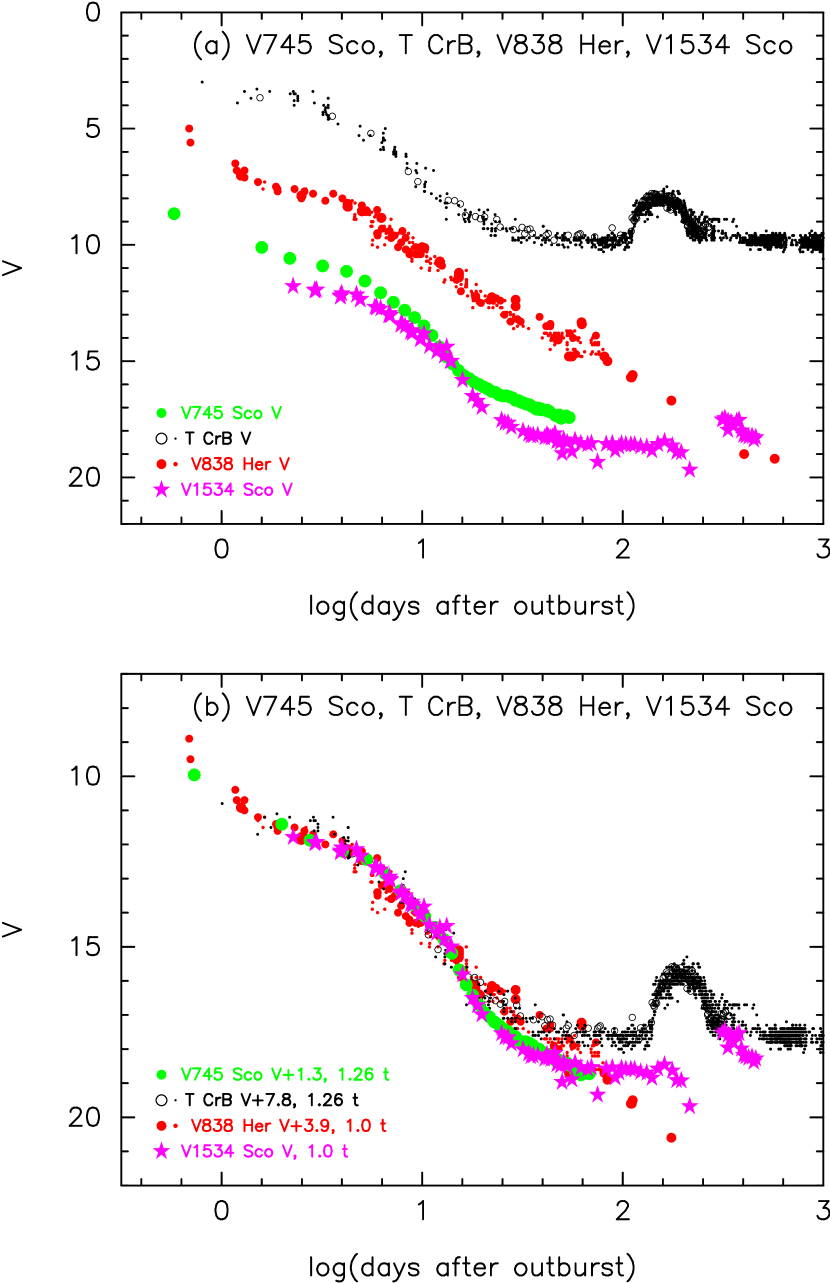
Figure 2: (a) $V$ and visual light curves of four novae, V745 Sco, T CrB, V838 Her, and V1534 Sco on a logarithmic timescale. Large symbols show the $V$ magnitudes, and small dots denote the visual magnitudes of each nova. (b) The four $V$ light curves overlap each other if we properly squeeze/stretch the timescales and shift up/down the $V$ and visual brightnesses.

2 Timescaling Law of Rapid-decline Novae

We analyze the light curves of V745 Sco, T CrB, V838 Her, and V1534 Sco, in this order. These novae do not follow the universal decline law of $F_{\nu}\propto t^{-1.75}$, but rather decline much faster, as $F_{\nu}\propto t^{-3.5}$ in the early decline phase (see filled black circles in Figure 1). Thus, we call them the rapid-decline (or V745 Sco) type novae. V745 Sco, T CrB, and V1534 Sco have a RG companion whereas V838 Her has a main-sequence (MS) companion. V745 Sco and T CrB are recurrent novae. Despite these differences, they show similar $V$ light curve shapes. Figure 2(a) shows the $V$ and visual light curves of these four novae on a logarithmic timescale. At the first glance, these novae show different shapes. However, V745 Sco and T CrB have similar shapes in the initial 20 days, and V838 Her and V1534 Sco decline similarly in the initial 15 days. If we stretch the first two light curves in the time direction by a factor of $1.26$, i.e., shift them rightward by $\Delta\log t=\log 1.26=0.1$, and shift all four light curves in the vertical direction, these four nova light curves almost overlap with each other, as shown in Figure 2(b). The vertical shifts $\Delta V(=1.3)$ and time-stretching factors $f_{\rm s}(=1.26)$ are shown in the figure, such as “V745 Sco $V+1.3$, $1.26~{}t$” for the V745 Sco light curve. Note that the time-stretching factor of $f_{\rm s}$ corresponds to the horizontal shift by $\Delta\log t=\log f_{\rm s}$ in Figure 2(b).

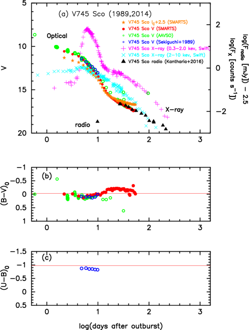
Figure 3: (a) The $V$ light curve of the V745 Sco 1989 (open blue circles from Sekiguchi et al., 1990) and 2014 (filled red circles from SMARTS and open green circles from AAVSO) outbursts are plotted on a logarithmic timescale. We add the $I_{C}$ magnitudes (filled orange stars) taken from SMARTS. We also include X-ray ($0.3-2.0$ keV with magenta pluses and $2.0-10$ keV with cyan crosses) data taken from Page et al. (2015) and radio (filled black triangles, GMRT at 610 MHz) data taken from Kantharia et al. (2016). (b) The $(B-V)_{0}$ color curve of the V745 Sco 1989 and 2014 outbursts. The horizontal solid red line denotes the intrinsic color of optically thick free-free emission, i.e., $(B-V)_{0}=-0.03$. (c) The $(U-B)_{0}$ color curve of the V745 Sco 1989 outburst. The horizontal solid red line denotes the intrinsic color of optically thick free-free emission, i.e., $(B-V)_{0}=-0.97$.

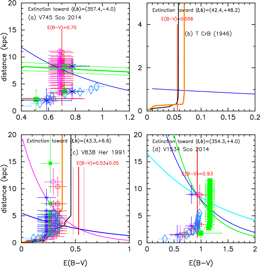
Figure 4: Distance-reddening relation toward (a) V745 Sco, (b) T CrB, (c) V838 Her, and (d) V1534 Sco. The thick blue lines denote (a) $(m-M)_{V}=16.6$, (b) $(m-M)_{V}=10.1$, (c) $(m-M)_{V}=13.7$, and (d) $(m-M)_{V}=17.6$, together with Equation (5). The vertical thick red lines denote the reddening of each nova, $E(B-V)$. Open red squares, filled green squares, blue asterisks, and open magenta circles with error bars represent the relations of Marshall et al. (2006) in the four directions close to each nova. The thick black and orange lines show the distance-reddening relations of Green et al. (2015, 2018), respectively. Open cyan-blue diamonds denote the distance-reddening relation taken from Özdörmez et al. (2016). In panel (a), the thick green line flanked by thin green lines indicates the distance-reddening relation of Equation (4). In panel (c), the thick magenta line denotes the distance-reddening relation given by the 1455 Å light curve fitting together with Equation (9). In panel (d), the green line denotes $(m-M)_{B}=18.55$ together with Equation (27) and the cyan line indicates $(m-M)_{I}=16.1$ together with Equation (31).

2.1 V745 Sco (1989, 2014)

V745 Sco is a recurrent nova with three recorded outbursts in 1937, 1989, and 2014 (e.g., Page et al., 2015). Figure 3 shows the $V$ and $I_{C}$ light curves, X-ray ($0.3-2.0$ keV soft band and $2-10$ keV hard band) light curves, radio (610 MHz) light curve, $(B-V)_{0}$, and $(U-B)_{0}$ color curves on a logarithmic timescale. This is similar to Figure 75 of Hachisu & Kato (2016b), but we added the $I_{C}$ data from SMARTS, the radio data from Kantharia et al. (2016), and the $V$ light curve from the American Association of Variable Star Observers (AAVSO). The 2014 outburst shows $m_{V,\rm max}=8.66$ (AAVSO), $t_{2}=2$ days, and $t_{3}=4$ days (e.g., Orio et al., 2015).

Table 1: Extinctions, distance moduli, and distances of selected novae

Object	Outburst	$E(B-V)$	$(m-M)_{V}$	$d$	$z$	$\log f_{s}$	Type
	Year			(kpc)	(pc)
CI Aql	(2000)	1.0	15.7	3.3	$-47$	$1.1$	normal
T CrB	(1946)	0.056	10.1	0.96	715	0.0	rapid
V407 Cyg	2010	1.0	16.1	3.9	$-33$	0.95	CSM
YY Dor	(2010)	0.12	18.9	50.0	—	0.6	normal
V838 Her	1991	0.53	13.7	2.6	310	0.1	rapid
RS Oph	(2006)	0.65	12.8	1.4	250	0.3	CSM
U Sco	(2010)	0.26	16.3	12.6	4680	0.0	normal
V745 Sco	(2014)	0.70	16.6	7.8	$-540$	0.0	rapid
V1534 Sco	2014	0.93	17.6	8.8	610	0.1	rapid
LMCN 2009a	(2014)	0.2	19.1	50.0	—	0.8	normal
LMCN 2012a	2012	0.15	19.0	50.0	—	0.1	rapid
LMCN 2013	2013	0.12	18.9	50.0	—	0.9	CSM
SMCN 2016	2016	0.08	16.8	20.4	$-13750$	0.6	normal
M31N 2008-12a	(2015)	0.30	24.8	780	—	0.0	rapid

Table 2: Decline rates of selected novae

Object	$\log f_{\rm s}$	$t_{2}$	$t_{3}$	$M_{V,\rm max}$	$P_{\rm orb}$	Companion	Reference of $t_{2}$ and $t_{3}$
		(day)	(day)		(day)
CI Aql	1.1	$25$	$32$	$-6.9$	0.618	subgiant	Strope et al. (2010)
T CrB	0.0	$4$	$6$	$-7.6$	227.6	red-giant	Strope et al. (2010)
V407 Cyg	0.95	$5.9$	$24$	$-9.0$	—	Mira	Munari et al. (2011b)
YY Dor	0.6	$4.0$	$10.9$	$-8.2$	—	—	Walter et al. (2012)
V838 Her	0.1	$1$	$4$	$-8.4$	0.2976	main-sequence	Strope et al. (2010)
RS Oph	0.3	$7$	$14$	$-8.0$	453.6	red-giant	Strope et al. (2010)
U Sco	0.0	$1.7$	$3.6$	$-8.7$	1.23	subgiant	Schaefer (2011)
V745 Sco	0.0	$2$	$4$	$-7.9$	—	red-giant	Orio et al. (2015)
V1534 Sco	0.1	$5.6$	$9.2$	$-5.8$	—	red-giant	Munari et al. (2017)
LMC N 2009a	0.8	$5.0$	$10.4$	$-8.5$	1.19	subgiant	Bode et al. (2016)
LMC N 2012a	0.1	$1.1$	$2.1$	$-8.3$	0.802	subgiant	Walter et al. (2012)
LMC N 2013	0.9	$21$	$47$	$-7.4$	—	—	present paper
SMC N 2016	0.6	$4.0$	$7.8$	$-8.3$	—	—	Aydi et al. (2018)
M31N 2008-12a	0.0	$1.65$	$2.37$	$-6.25$	—	—	Darnley et al. (2016)

Table 3: White dwarf masses of selected novae

Object	$\log f_{\rm s}$	$M_{\rm WD}$	$M_{\rm WD}$	$M_{\rm WD}$	$M_{\rm WD}$
		$f_{\rm s}$	UV 1455 Å	$t_{\rm SSS-on}$	$t_{\rm SSS-off}$
		($M_{\sun}$)	($M_{\sun}$)	($M_{\sun}$)	($M_{\sun}$)
CI Aql	1.1	$1.18$	—	—	—
T CrB	0.0	$1.38$	—	—	—
V407 Cyg	0.95	$1.22$	—	—	—
YY Dor	0.6	$1.29$	—	—	—
V838 Her	0.1	$1.37$	$1.37$	—	—
RS Oph	0.3	$1.35$	$1.35$	$1.35$	$1.35$
U Sco	0.0	$1.37$	—	$1.37$	$1.37$
V745 Sco	0.0	$1.38$	—	$1.385$	$1.385$
V1534 Sco	0.1	$1.37$	—	—	—
LMC N 2009a	0.8	$1.25$	—	$1.25$	$1.25$
LMC N 2012a	0.1	$1.37$	—	—	—
LMC N 2013	0.9	$1.23$	—	—	—
SMC N 2016	0.6	$1.29$	—	—	—
M31N 2008-12a	0.0	$1.38$	—	$1.38$	$1.38$

2.1.1 Reddening and distance

The galactic coordinates of V745 Sco are $(l,b)=(357\fdg 3584,-3\fdg 9991)$. The NASA/IPAC galactic dust absorption map gives $E(B-V)=0.71\pm 0.02$ toward V745 Sco, which is based on the galactic dust extinction of Schlafly & Finkbeiner (2011). Banerjee et al. (2014) suggested that the extinction for V745 Sco is $E(B-V)=0.70$ on the basis of the galactic dust extinction of Schlafly & Finkbeiner (2011) and Marshall et al. (2006). Orio et al. (2015) fitted the X-ray spectrum 10 days after the discovery of the 2014 outburst with a model spectrum and obtained the hydrogen column density of $N_{\rm H}=(6.9\pm 0.9)\times 10^{21}$ cm^-2, which corresponds to the extinction of $E(B-V)=N_{\rm H}/6.8\times 10^{21}$ cm${}^{-2}=1.0\pm 0.1$ (Güver & Özel, 2009) or $E(B-V)=N_{\rm H}/8.3\times 10^{21}=0.83\pm 0.1$ (Liszt, 2014). Hachisu & Kato (2016b) adopted $E(B-V)=0.70\pm 0.1$, mainly from the results of Banerjee et al. (2014) and the NASA/IPAC galactic dust absorption map. We adopt $E(B-V)=0.70\pm 0.1$, pursuant to Hachisu & Kato (2016b).

The intrinsic colors are obtained from

$$(B-V)_{0}=(B-V)-E(B-V),$$ (1)

$$(U-B)_{0}=(U-B)-0.64E(B-V),$$ (2)

where the factor of $0.64$ is taken from Rieke & Lebofsky (1985). The intrinsic color $(B-V)_{0}$ of AAVSO and Sekiguchi et al. (1990) are systematically 0.1 and 0.3 mag redder than those of SMARTS, the data of which are taken from Page et al. (2015). Therefore, we shift them up by 0.1 and 0.3 mag, respectively, in Figure 3(b).

There are sometimes substantial differences among colors of novae observed at different observatories. Such differences could originate from, for example, slight differences in response functions of each filter, different comparison stars, and so on. We do not know the exact origin of the difference in this nova, but we suppose that the $(B-V)_{0}$ color is close to $-0.03$ in the early decline phase before the nebular phase. This is because nova spectra are dominated by optically thick free-free emission (continuum) and its intrinsic color $(B-V)_{0}$ is $-0.03$ ($F_{\nu}\propto\nu^{2/3}$, see Hachisu & Kato, 2014). The color of SMARTS is close to this value in the very early phase. We regard that the intrinsic colors of SMARTS are reasonable but the colors of AAVSO and Sekiguchi et al. (1990) deviate from those of SMARTS. Thus, we correct the intrinsic $(B-V)_{0}$ colors of AAVSO and Sekiguchi et al. by 0.1 and 0.3 mag, respectively.

The distance to V745 Sco was estimated by Schaefer (2009) to be $d=7.8$ kpc from the orbital period of $P_{\rm orb}=510\pm 20$ days and the corresponding Roche lobe size. However, this period was not confirmed by Mróz et al. (2014), and thus, we do not use the method based on the Roche lobe size.

Mróz et al. (2014) detected semi-regular pulsations of the RG companion (with periods of 136.5 days and 77.4 days). Hachisu & Kato (2016b) estimated the distance from the period-luminosity relation for pulsating red-giants, i.e.,

$$M_{K}=-3.51\times(\log P({\rm day})-2.38)-7.25,$$ (3)

with an error of $\sim 0.2$ mag (Whitelock et al., 2008). Hachisu & Kato (2016b) obtained the absolute $K$ magnitude of $M_{K}=-6.39\pm 0.2$ for the fundamental 136.5-day pulsation from the data of Mróz et al. (2014). Adopting an average $K$ mag of $m_{K}=8.33$ mag (Hoard et al., 2002), Hachisu & Kato (2016b) obtained $d=7.8\pm 0.8$ kpc for $E(B-V)=0.70$ from

$$(m-M)_{K}=0.353\times E(B-V)+5\log~{}(d/1~{}{\rm kpc})+10,$$ (4)

where they adopted the reddening law of $A_{K}=0.353\times E(B-V)$ (Cardelli et al., 1989). Their new distance is accidentally identical to Schaefer’s value of 7.8 kpc. The vertical distance from the galactic plane is approximately $z=-540$ pc, being significantly above the scale height of galactic matter distribution ($z=\pm 125$ pc, see, e.g., Marshall et al., 2006). Thus, it is likely that V745 Sco belongs to the galactic bulge.

We plot the distance-reddening relation of Equation (4) with a thick green line flanked by thin green lines in Figure 4(a). In the same figure, we add the reddening of $E(B-V)=0.70$, indicated by the vertical thick red line. The thick green line and red line cross at $d=7.8$ kpc. Hachisu & Kato (2016b) obtained the distance modulus in the $V$ band, $(m-M)_{V}=16.6\pm 0.2$, which was calculated from

$$(m-M)_{V}=5\log(d/{\rm 10~{}pc})+3.1E(B-V),$$ (5)

where the factor of $3.1$ is taken from Rieke & Lebofsky (1985). We also plot this distance-reddening relation of Equation (5) with the thick blue line in Figure 4(a). Note that this relation of $(m-M)_{V}=16.6$ is not an independent relation of $(m-M)_{K}=m_{K}-M_{K}=8.33-(-6.39)=14.72$ because it is just derived from Equation (5) together with $E(B-V)=0.70$ and $d=7.8$ kpc.

After Hachisu & Kato’s (2016b) paper was published, Özdörmez et al. (2016) obtained distance-reddening relations toward 46 novae based on the unique position of red clump giants in the color-magnitude diagram. Their distance-$E(J-K)$ relation toward V745 Sco is plotted in their Figure C2. They estimated the distance to V745 Sco to be $d=3.5\pm 0.85$ kpc for the assumed reddening of $E(B-V)=0.84\pm 0.15$ (or $E(J-K)=0.44\pm 0.07$). This distance of $d=3.5$ kpc is much shorter than our distance of $d=7.8$ kpc. We converted their distance-$E(J-K)$ relation to a distance-$E(B-V)$ relation using the conversion of $E(J-K)=0.524E(B-V)$ (Rieke & Lebofsky, 1985), and plotted it with the open cyan-blue diamonds in Figure 4(a).

We also plot the distance-reddening relations given by Marshall et al. (2006), who published a three-dimensional (3D) dust extinction map of our galaxy in the direction of $-100\fdg 0\leq l\leq 100\fdg 0$ and $-10\fdg 0\leq b\leq+10\fdg 0$ with grids of $\Delta l=0\fdg 25$ and $\Delta b=0\fdg 25$, where $(l,b)$ are the galactic coordinates. Figure 4(a) shows four relations in the directions close to V745 Sco, i.e., $(l,b)=(357\fdg 25,-4\fdg 00)$ (open red squares), $(357\fdg 50,-4\fdg 00)$ (filled green squares), $(357\fdg 25,-3\fdg 75)$ (blue asterisks), and $(357\fdg 50,-3\fdg 75)$ (open magenta circles), with error bars. The closest one is that of the open red squares. The reddening saturates to $E(B-V)\sim 0.7\pm 0.1$ at the distance of $d\sim 3-4$ kpc. This is consistent with the result of the NASA/IPAC galactic two-dimensional (2D) dust absorption map, $E(B-V)=0.71\pm 0.02$. The distance-reddening relation given by Özdörmez et al. (2016) consistently follows the relation given by Marshall et al. (2006) until $E(B-V)=0.7$, but does not saturate at the distance of $d\sim 3-4$ kpc. Their reddening linearly increases to $E(B-V)=1.0$. This is the reason why Özdörmez et al. (2016) obtained a much smaller distance for V745 Sco.

The angular resolution of the map of Marshall et al. is 0$\fdg$25=15$\farcm$ Marshall et al. used only giants in their analysis, and thus the dust map they produced has little information for the nearest kiloparsec. The effective resolution of the NASA/IPAC galactic 2D dust absorption map depends on the few-arcminute resolution of the IRAS $100~{}\mu$m image and the $\sim$1 degree COBE/DIRBE dust temperature map, which is considerably larger than the molecular cloud structure observed in the interstellar medium. Özdörmez et al. (2016) used red clump giants. The number density of red clump giants is smaller than that of giants that Marshall et al. used. Therefore, the angular resolution of Özdörmez et al. (2016) could be less than that of Marshall et al. (2006). Although Özdörmez et al. (2016) showed that the distance-reddening relation toward WY Sge is not significantly different for the four resolutions of 0$\fdg$3, 0$\fdg$4, 0$\fdg$5, and 0$\fdg$8, we adopt $E(B-V)=0.70$ for V745 Sco in the present study, following Marshall et al. (2006) and the NASA/IPAC galactic 2D dust absorption map. We will demonstrate that this reddening of $E(B-V)=0.70$ is reasonable by comparing various properties of V745 Sco with those of other novae. We summarize various properties of V745 Sco in Tables 1, 2, and 3.

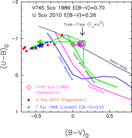
Figure 5: Color-color diagrams of V745 Sco (1989), U Sco (2010), and T Pyx (1966). These color-color diagrams are similar to Figure 36 of Hachisu & Kato (2016b), but we reanalyzed the data. The open black square denotes the position of optically thin free-free emission ($F_{\nu}\propto\nu^{0}$). See the text for sources of observational data.

2.1.2 Color-color diagram

Figure 5 shows the color-color diagram of V745 Sco (1989) in outburst for the reddening of $E(B-V)=0.70$. We add other two tracks of U Sco (2010) and T Pyx (1966) for comparison. There are only six data (magenta open circles) of V745 Sco but five of the six data are located at or near the point of $(B-V)_{0}=+0.13$ and $(U-B)_{0}=-0.87$ denoted by the open black square labeled “free-free ($F_{\nu}\propto\nu^{0}$).” This point corresponds to the position of optically thin free-free emission (Hachisu & Kato, 2014). These positions of the data in the color-color diagram are consistent with the fact that the ejecta had already been optically thin when these data were obtained. This is consistent with the value of $E(B-V)=0.70$.

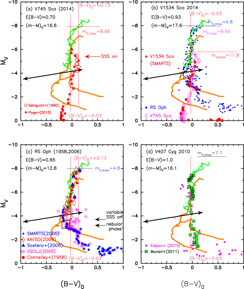
Figure 6: Color-magnitude diagrams of (a) V745 Sco, (b) V1534 Sco, (c) RS Oph, and (d) V407 Cyg. The thick green lines show the template track of V1668 Cyg and the thick orange lines represent that of LV Vul (taken from Hachisu & Kato, 2016b). The two-headed black arrow indicates the locations of inflection (for slow novae) or turning point of color-magnitude tracks (Hachisu & Kato, 2016b). The vertical thin red lines indicate the color of optically thick, $(B-V)_{0}=-0.03$, and optically thin, $(B-V)_{0}=+0.13$, free-free emission. See the text for more detail.

2.1.3 Color-magnitude diagram

Using $E(B-V)=0.70$ and $(m-M)_{V}=16.6$ ($d=7.8$ kpc), we plot the color-magnitude diagram, $(B-V)_{0}$-$M_{V}$, of V745 Sco in Figure 6(a). The green lines denote the template track of V1668 Cyg and the orange lines represent that of LV Vul (taken from Hachisu & Kato, 2016b). The two-headed black arrow indicates the locations of inflection (for slow novae) or turning point of color-magnitude tracks (Hachisu & Kato, 2016b). In the very early phase, the track of V745 Sco follows the vertical solid red line of $(B-V)_{0}=-0.03$, which is the intrinsic color of optically thick free-free emission (see, e.g., Hachisu & Kato, 2014). This trend is similar to other classical novae such as V1668 Cyg.

The color increases to $(B-V)_{0}=+0.13$ four days after the discovery; the discovery date is JD 2456695.194 (e.g., Page et al., 2015). This is the intrinsic color of optically thin free-free emission (Hachisu & Kato, 2014). The color change from $(B-V)_{0}=-0.03$ to $(B-V)_{0}=+0.13$ indicates that the ejecta became transparent (optically thin) after this date. The color then gradually becomes blue and reaches $(B-V)_{0}=-0.2$ in the very late phase. This is because strong emission lines begin to contribute to the $B$ band flux (Hachisu & Kato, 2014). The intrinsic color of V745 Sco is redder than $(B-V)_{0}\gtrsim-0.2$ throughout the outburst. This is a common property among symbiotic nova systems with a RG companion, as shown in Figures 6(b), (c), and (d).

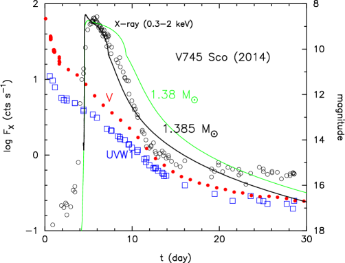
Figure 7: Model light curve fitting of the supersoft X-ray flux ($0.3-2.0$ keV denoted by open black circles) for the V745 Sco 2014 outburst. The start of day (horizontal axis) is the discovery date (JD 2456695.194). We also include the $V$ (filled red circles) and UVW1 (open blue squares) magnitudes. All the observational data are taken from Page et al. (2015). A $1.385~{}M_{\sun}$ WD model (solid black line) reasonably reproduces the observed supersoft X-ray flux rather than a $1.38~{}M_{\sun}$ WD model (solid green line).

2.1.4 Model light curve of supersoft X-ray

The SSS phase of V745 Sco started just four days after the discovery (Figure 7). If the optical brightness reaches its maximum at the discovery date, this turn-on time of SSS is the earliest record ($t_{\rm SSS-on}=4$ days) among novae. The second shortest record ($t_{\rm SSS-on}=6$ days) is the 1-yr recurrence period nova, M31N 2008-12a (Henze et al., 2015). Kato et al. (2017) modeled time-evolutions of such very-short-timescale novae and obtained a reasonable light curve fit with a $1.38~{}M_{\sun}$ WD for M31N 2008-12a. The earlier appearance of SSS for V745 Sco suggests a more massive WD than that of M31N 2008-12a. We have modeled time-evolutions similar to the calculation of Kato et al. (2017) and obtained a reasonable fit (solid black line) with the supersoft X-ray light curve (open black circles), as shown in Figure 7. We plot the supersoft X-ray flux ($0.3-2.0$ keV count rates of the Swift XRT) as well as the $V$ magnitude and Swift UVW1 magnitude light curves. All the observational data are taken from Page et al. (2015). Our obtained WD mass is $1.385~{}M_{\sun}$, more massive than $1.38~{}M_{\sun}$ for M31N 2008-12a. It is unlikely that these WDs were born as massive as they are ($1.38~{}M_{\sun}$ or $1.385~{}M_{\sun}$, see, e.g., Doherty et al., 2015). We suppose that these WDs have grown in mass.

The X-ray flux of our model is calculated from blackbody spectra of the photospheric temperature ($T_{\rm ph}$) and radius ($R_{\rm ph}$), and the detailed flux itself is thus not so accurate, but the duration of the SSS phase (rise and decay of the flux) is reasonably reproduced. Nomoto (1982) showed that, if a WD has a carbon-oxygen core and its mass reaches $\sim 1.38~{}M_{\sun}$ or more, the WD explodes as a SN Ia. Therefore, V745 Sco is one of the most promising candidates of SN Ia progenitors.

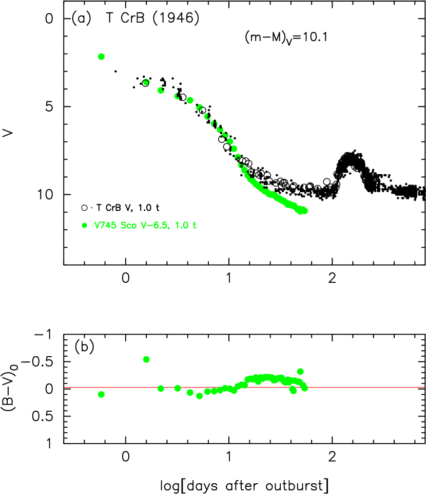
Figure 8: (a) The $V$ (open black circles) and visual (black dots) light curves of the T CrB 1946 outburst are plotted on a logarithmic timescale as well as the light/color curves of the V745 Sco 2014 outburst (filled green circles). The timescales of these two novae are the same, i.e., the timescaling factor of T CrB is $f_{\rm s}=1.0$ with respect to that of V745 Sco. The $V$ light curve of V745 Sco is shifted up by 6.5 mag. The vertical shift and timescaling are written as “V745 Sco V$-$6.5, 1.0 t” in the figure. (b) $(B-V)_{0}$ color curve of the V745 Sco 2014 outburst. The horizontal solid red line denotes the color of optically thick free-free emission, i.e., $(B-V)_{0}=-0.03$.

2.2 T CrB (1946)

T CrB is also a recurrent nova with two recorded outbursts in 1866 and 1946 (e.g., Schaefer, 2010). The orbital period was obtained to be $P_{\rm orb}=227.6$ days (Fekel et al., 2000). Figure 8 shows the $V$ and visual light curves of T CrB on a logarithmic timescale. The $V$ and visual light curves show a smooth decline and a late secondary maximum. The origin of the secondary maximum was discussed by Hachisu & Kato (2001b) in terms of an irradiated tilting disk. They also estimated the WD mass of T CrB to be $M_{\rm WD}=1.37\pm 0.01~{}M_{\sun}$ from the model light curve fitting. The peak $V$ magnitude of T CrB reaches $m_{V,\rm max}=2.5$ (Schaefer, 2010). The decline rate is characterized by $t_{2}=4$ and $t_{3}=6$ days (e.g., Strope et al., 2010). Figure 8 also shows the $V$ light curve of V745 Sco on the same timescale, but its brightness is shifted up by 6.5 mag. These two light curves are very similar until $\sim 10$ days after the outbursts.

2.2.1 Distance and reddening

The distance was estimated by various authors (e.g., Bailey, 1981; Harrison et al., 1993; Belczyński & Mikołajewska, 1998; Schaefer, 2010), and summarized by Schaefer (2010) to be $d=900\pm 200$ pc. In the present paper, we adopt $d=960\pm 150$ pc after Belczyński & Mikołajewska (1998). T CrB shows an ellipsoidal variation in the quiescent light curve, suggesting that the RG companion almost fills its Roche lobe. Assuming that the RG companion just fills its Roche lobe, Belczyński & Mikołajewska (1998) obtained the absolute brightness of the RG companion and estimated the distance.

For the reddening toward T CrB, whose galactic coordinates are $(l,b)=(42\fdg 3738,+48\fdg 1647)$, the NASA/IPAC galactic 2D dust absorption map gives $E(B-V)=0.056\pm 0.003$ toward T CrB. If we adopt $E(B-V)=0.056$ toward T CrB, then we calculate the distance modulus in the $V$ band to be $(m-M)_{V}=10.1\pm 0.3$ from Equation (5). We plot the distance-reddening relations (black and orange lines) of Green et al. (2015, 2018), respectively, in Figure 4(b). Green et al. (2015) published data for the galactic 3D extinction map, which covers a wide range of the galactic coordinates (over three quarters of the sky) with grids of 3$\farcm$4 to 13$\farcm$7 and a maximum distance resolution of 25%. Note that the values of $E(B-V)$ reported by Green et al. could have an error of $0.05-0.1$ mag compared with the 2D dust extinction maps. The reddening saturates at the distance of $0.7$ kpc and the set of $d=0.96$ kpc and $E(B-V)=0.056$ is consistent with the relation of Green et al. (2015). Then, the vertical distance from the galactic plane is approximately $z=+715$ pc. We summarize various properties of T CrB in Tables 1, 2, and 3.

2.2.2 Absolute magnitudes and diversity in the late phase

Figure 8(a) shows that the global decline timescales of T CrB and V745 Sco are very similar and their $V$ light curves almost overlap with each other if we shift the $V$ light curve of V745 Sco vertically up by 6.5 mag. The $V$ light curves of the two novae deviate in the late phase of the outbursts. This is caused by different contributions of the RG companions and accretion disks.

The distance modulus in the $V$ band is calculated to be $(m-M)_{V}=10.1\pm 0.3$ from Equation (5), together with $d=960\pm 150$ pc and $E(B-V)=0.056\pm 0.003$. For T CrB and V745 Sco, we have the following relation

$$(m - M)_{V,\rm T~{}CrB}=10.1\pm 0.3$$ (6)

$$= (m-M+\Delta V)_{V,\rm V745~{}Sco}$$ (7)

$$= (16.6\pm 0.2)+(-6.5\pm 0.1)=10.1\pm 0.3,$$ (8)

where we adopt $(m-M)_{V,\rm V745~{}Sco}=16.6\pm 0.2$, as obtained in Section 2.1, and the vertical shift of the V745 Sco $V$ light curve is $\Delta V=-6.5\pm 0.1$ because we change $\Delta V$ in steps of $0.1$ mag and searched for the best overlap. This clearly shows that the two novae have the same absolute magnitudes within the ambiguity of $\pm 0.3$ mag when the timescales are the same. The difference in the apparent magnitudes is due to the differences in the distance and absorption.

In general, there are two sources of $(m-M)_{V}$ ambiguities in our fitting procedure: one is the error in $(m-M)_{V}$ of the template nova and the other is the ambiguity of vertical fit of $\Delta V$. For the vertical fit, we change $\Delta V$ in steps of 0.1 mag and search for the best overlap by eye. Its error is typically 0.1 mag (sometimes 0.2 mag) unless the $V$ data are substantially scattered. The $(m-M)_{V}$ ambiguity of the template nova is dependent on each template (typically 0.2 or 0.3 mag). Thus, the errors of distance moduli $(m-M)_{V}$ are 0.2 or 0.3 mag unless otherwise specified.

Figure 9: Same as Figure 8, but we plot the visual (red dots) and $V$ (filled red circles), UV 1455 Å flux (large open red circles), and $(B-V)_{0}$ color curves (filled red circles) of V838 Her (red symbols) as well as the visual and $V$ light curves of T CrB (black symbols), and the $V$ light curve and $(B-V)_{0}$ color curve of V745 Sco (blue symbols). The timescales of T CrB and V745 Sco are stretched by a factor of $1.26$, i.e., the timescaling factor of V838 Her is $f_{\rm s}=1.26$ with respect to that of V745 Sco. (a) The $V$ light curve of T CrB is shifted down by 3.8 mag and that of V745 Sco is shifted up by 2.7 mag. These shifts are indicated by “T CrB V+3.8, 1.26 t” and “V745 Sco V$-$2.7, 1.26 t” in the figure. (b) $(B-V)_{0}$ color curves of V838 Her and V745 Sco.

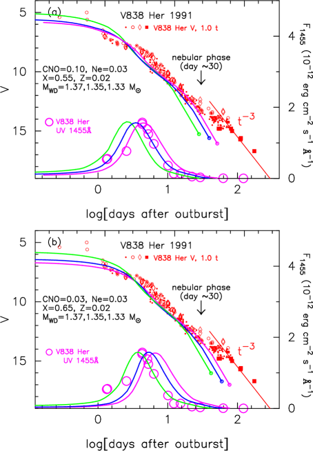
Figure 10: $V$ and UV 1455 Å light curve fittings for V838 Her. The sources of optical and UV 1455 Å data are the same as those in Figure 8 of Kato et al. (2009). (a) We plot three WD mass models of $1.37~{}M_{\sun}$ (green), $1.35~{}M_{\sun}$ (blue), and $1.33~{}M_{\sun}$ (magenta) for the chemical composition of Ne nova 2 (Hachisu & Kato, 2010). The open circles at the right edge of the model light curves denote the epoch when the optically thick winds stop. We add a straight solid red line labeled “$t^{-3}$” in the figure from the theoretical point of view. If the ejecta were expanding homologously, i.e., free expansion, the flux would evolve as $F_{\nu}\propto t^{-3}$. (b) We plot three WD mass models of $1.37~{}M_{\sun}$ (green), $1.35~{}M_{\sun}$ (blue), and $1.33~{}M_{\sun}$ (magenta), but for the different chemical composition of Ne nova 3 (Hachisu & Kato, 2016a).

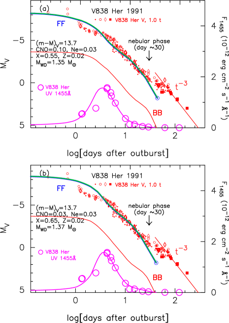
Figure 11: Same as Figure 10, but we plot the best-fit models in the absolute $V$ magnitude: (a) the $1.35~{}M_{\sun}$ WD with the chemical composition of Ne nova 2 and (b) the $1.37~{}M_{\sun}$ WD with the chemical composition of Ne nova 3. Three $V$ light curves are plotted for the blackbody flux (solid red line labeled “BB”), free-free flux (solid blue line labeled “FF”), and the total flux (solid green) of blackbody and free-free emission. The open blue circle at the right end of free-free flux denotes the epoch when the optically thick winds stop.

2.3 V838 Her 1991

V838 Her is a very fast nova with $t_{2}=1$ day and $t_{3}=4$ days, and its peak brightness reached $m_{V,\rm max}=5.3$ (Strope et al., 2010). The orbital period was obtained to be $P_{\rm orb}=0.2976$ days (Ingram et al., 1992; Leibowitz et al., 1992). Figure 9 shows the $V$ and visual light curves of V838 Her on a logarithmic timescale. This figure also shows the $V$ light and $B-V$ color curves of V745 Sco and the $V$ and visual light curves of T CrB to demonstrate the resemblance among the three novae. The reddening toward V838 Her was estimated by several authors (e.g., Matheson et al., 1993; Harrison et al., 1994; Vanlandingham et al., 1996; Kato et al., 2009) to lie between $E(B-V)=0.3-0.7$. Of these values, we adopt $E(B-V)=0.53\pm 0.05$ after Kato et al. (2009), which was obtained from the 2175 Å feature of the UV spectra of V838 Her. Kato et al. (2009) also derived the distance of $d=2.7\pm 0.5$ kpc from the UV 1455 Å flux fitting and the WD mass of $M_{\rm WD}=1.35\pm 0.02~{}M_{\sun}$ from the model light curve fitting.

2.3.1 Model light curve fitting

We briefly explain the $V$ light curve and UV 1455 Å light curve fitting of novae. Nova spectra are dominated by the free-free emission the after optical maximum (e.g., Gallagher & Ney, 1976; Ennis et al., 1977). This free-free emission comes from optically thin plasma outside the photosphere. Hachisu & Kato (2006) calculated free-free emission model light curves of novae and showed that theoretical light curves reproduce well observed NIR/optical light curves of several classical novae from near the peak to the nebular phase. These free-free emission model light curves are calculated from the nova evolution models based on the optically thick wind theory (Kato & Hachisu, 1994). Their numerical models provide the photospheric temperature ($T_{\rm ph}$), radius ($R_{\rm ph}$), velocity ($v_{\rm ph}$), and wind mass-loss rate ($\dot{M}_{\rm wind}$) of a nova hydrogen-rich envelope (mass of $M_{\rm env}$) for a specified WD mass ($M_{\rm WD}$) and chemical composition of the hydrogen-rich envelope. The free-free emission model light curves are calculated by Equations (9) and (10) in Hachisu & Kato (2006).

Envelope chemical composition of their model is given by the form of $(X,Y,X_{\rm CNO},X_{\rm Ne},Z)$. Here, $X$ is the hydrogen content, $Y$ the helium content, $X_{\rm CNO}$ the abundance of carbon, nitrogen, and oxygen, $X_{\rm Ne}$ the neon content, and $Z=0.02$ the heavy element (heavier than helium) content by weight, in which carbon, nitrogen, oxygen, and neon are also included with the solar composition ratios (Hachisu & Kato, 2006). The chemical composition of the V838 Her ejecta was estimated by Vanlandingham et al. (1996), Vanlandingham et al. (1997), and Schwarz et al. (2007). The results are summarized in Table 2 of Kato et al. (2009). In this study, we calculated two cases, “Ne nova 2” ($X=0.55$, $Y=0.30$, $Z=0.02$, $X_{\rm CNO}=0.10$, and $X_{\rm Ne}=0.03$) (Hachisu & Kato, 2010) and “Ne nova 3” ($X=0.65$, $Y=0.27$, $Z=0.02$, $X_{\rm CNO}=0.03$, and $X_{\rm Ne}=0.03$) (Hachisu & Kato, 2016a), both of which are close to the estimates mentioned above.

In Figure 10(a), we plot three WD mass models: $1.37~{}M_{\sun}$ (green), $1.35~{}M_{\sun}$ (blue), and $1.33~{}M_{\sun}$ (magenta) for Ne nova 2. The open circles at the right edge of model light curves denote the epoch when the optically thick winds stop. We tabulate these three free-free emission model light curves in Table 4. A more massive WD evolves faster. The UV 1455 Å band is an emission-line-free narrow band (20 Å width centered at 1455 Å) invented by Cassatella et al. (2002) based on the IUE spectra of novae. This band represents continuum flux at UV well and is useful for model light curve fitting. Hachisu & Kato (2006, 2010, 2015, 2016a) calculated UV 1455 Å model light curves for various WD masses and chemical compositions of the hydrogen-rich envelope, assuming blackbody emission at the photosphere. In Figure 10(a), the best-fit model among the three WD mass models is the $1.35~{}M_{\sun}$ WD model (solid blue lines).

In Figure 10(b), we also plot three WD mass models: $1.37~{}M_{\sun}$ (green), $1.35~{}M_{\sun}$ (blue), and $1.33~{}M_{\sun}$ (magenta), but for the different chemical composition of Ne nova 3. We tabulate these three free-free emission model light curves in Table 5. For this chemical composition, the best-fit model among the three WD mass models is the $1.37~{}M_{\sun}$ WD model (solid green lines).

We add a straight solid red line labeled “$t^{-3}$” in these figures from the theoretical point of view. After the optically thick winds stop at the open circle (right edge of the free-free model $V$ light curve), the ejecta mass $M_{\rm ej}$ is virtually constant with time because of no mass supply from the WD. If the ejecta were expanding homologously, i.e., free expansion, the free-free emission flux would evolve as $F_{\nu}\propto t^{-3}$ (see, e.g., Woodward et al., 1997; Hachisu & Kato, 2006). We plot this trend as a guide in the later decline phase.

After the optically thick winds stop, the photosphere quickly shrinks, the photospheric temperature increases to emit high-energy photons, and the nova enters the nebular phase. This nova entered the nebular phase approximately 30 days after the outburst, i.e., at least by UT 1991 April 23 (e.g., Williams et al., 1994; Vanlandingham et al., 1996). In this case, the neon forbidden lines had grown to become comparable in strength to H$\alpha$. In the nebular phase, strong emission lines contribute to the $V$ magnitude. As a result, the model light curve deviates significantly from the observational $V$ light curve, as shown in Figure 10, because the model $V$ light curve does not include the effect of emission lines, but rather represents only continuum (free-free) emission.

Fitting our model to the observed UV 1455 Å flux, we have the following relation:

$$-2.5\log\left(F_{\lambda}^{\rm obs}/F_{\lambda}^{\rm mod}\right)=R_{\lambda}E(B-V)+5\log\left({{d}\over{10~{}{\rm kpc}}}\right),$$ (9)

where $F_{\lambda}^{\rm mod}$ is the model flux at the distance of $d=10$ kpc, $F_{\lambda}^{\rm obs}$ is the observed flux, the absorption is calculated from $A_{\lambda}=R_{\lambda}E(B-V)$, and $R_{\lambda}=8.3$ for $\lambda=1455$ Å (Seaton, 1979). For the $1.35~{}M_{\sun}$ WD model in Figure 10(a), $F_{1455}^{\rm obs}=5.0$ and $F_{1455}^{\rm mod}=21.0$, in units of $10^{-12}$ erg cm^-2 s^-1 Å^-1, at the upper bound of Figure 10(a), whereas for the $1.37~{}M_{\sun}$ WD model in Figure 10(b), $F_{1455}^{\rm obs}=5.0$ and $F_{1455}^{\rm mod}=20.0$. Substituting $E(B-V)=0.53$ into Equation (9), both the cases give $d=2.6-2.7$ kpc. This value is consistent with the estimate by Kato et al. (2009). The distance calculated by our model fitting hardly depends on the assumed chemical composition. The distance modulus in the $V$ band is calculated from Equation (5) to be $(m-M)_{V}=13.7\pm 0.3$ for V838 Her. The vertical distance from the galactic plane is approximately $z=+310$ pc, because the galactic coordinates of V838 Her are $(l,b)=(43\fdg 3155,+6\fdg 6187)$. We summarize various properties of V838 Her in Tables 1, 2, and 3.

Assuming that $(m-M)_{V}=13.7$, we plot the absolute $V$ magnitude light curve of V838 Her in Figure 11. The total flux (solid green line) of the $V$ band consists of the two parts; one is the flux of free-free emission (solid blue line labeled “FF”), which comes from optically thin plasma outside the photosphere, and the other is the photospheric emission (solid red line labeled “BB”), which is approximated by blackbody emission. It is clear that the flux of free-free emission is much larger than that of blackbody emission. Thus, the free-free emission dominates the continuum spectra of very fast novae.

If we average the hydrogen contents of the three results mentioned above, i.e., Vanlandingham et al. (1996), Vanlandingham et al. (1997), and Schwarz et al. (2007), we obtain $X=(0.78+0.59+0.562)/3=0.644$. This value is close to our case of Ne nova 3 ($X=0.65$, $Y=0.27$, $Z=0.02$, $X_{\rm CNO}=0.03$, and $X_{\rm Ne}=0.03$). Therefore, we adopt the $1.37~{}M_{\sun}$ WD for V838 Her.

Table 4: Free-free Light Curves of Ne Novae 2

$m_{\rm ff}$	1.33$M_{\sun}$	1.35$M_{\sun}$	1.37$M_{\sun}$
(mag)	(day)	(day)	(day)
4.500	0.0	0.0	0.0
4.750	0.4617	0.6000	0.4350
5.000	0.8397	1.019	0.7630
5.250	1.173	1.354	1.074
5.500	1.575	1.673	1.385
5.750	1.992	2.019	1.694
6.000	2.396	2.399	2.007
6.250	2.786	2.742	2.328
6.500	3.189	3.075	2.628
6.750	3.591	3.408	2.871
7.000	4.001	3.736	3.137
7.250	4.403	4.041	3.380
7.500	4.810	4.346	3.606
7.750	5.235	4.643	3.819
8.000	5.717	4.959	4.044
8.250	6.355	5.326	4.295
8.500	7.079	5.766	4.594
8.750	7.949	6.299	4.943
9.000	8.922	6.945	5.373
9.250	10.05	7.683	5.857
9.500	11.45	8.533	6.443
9.750	13.13	9.533	7.097
10.00	14.94	10.76	7.918
10.25	16.83	12.15	8.828
10.50	18.68	13.51	9.748
10.75	20.56	14.85	10.62
11.00	22.30	16.25	11.40
11.25	23.73	17.56	12.23
11.50	25.19	18.75	13.10
11.75	26.75	20.01	14.03
12.00	28.39	21.35	15.01
12.25	30.13	22.76	16.05
12.50	31.97	24.26	17.15
12.75	33.93	25.84	18.31
13.00	35.99	27.52	19.55
13.25	38.18	29.30	20.86
13.50	40.50	31.19	22.24
13.75	42.96	33.18	23.71
14.00	45.57	35.30	25.27
14.25	48.32	37.54	26.91
14.50	51.24	39.91	28.66
14.75	54.34	42.42	30.50
15.00	57.61	45.08	32.46
X-ray	23.4	14.3	7.80
$\log f_{\rm s}$	$+0.10$	0.0	$-0.12$
$M_{\rm w}$	$2.2$	$1.8$	$1.4$

Table 5: Free-free Light Curves of Ne Novae 3

$m_{\rm ff}$	1.33$M_{\sun}$	1.35$M_{\sun}$	1.37$M_{\sun}$
(mag)	(day)	(day)	(day)
3.750	0.0	0.0	0.0
4.000	0.4317	0.4570	0.3855
4.250	0.9427	0.9240	0.9118
4.500	1.481	1.388	1.420
4.750	2.023	1.914	1.889
5.000	2.594	2.477	2.324
5.250	3.173	3.008	2.752
5.500	3.686	3.426	3.140
5.750	4.176	3.861	3.498
6.000	4.665	4.270	3.870
6.250	5.128	4.653	4.180
6.500	5.621	5.042	4.487
6.750	6.130	5.430	4.798
7.000	6.622	5.842	5.058
7.250	7.129	6.232	5.320
7.500	7.646	6.621	5.605
7.750	8.221	7.041	5.930
8.000	8.886	7.557	6.296
8.250	9.698	8.153	6.707
8.500	10.63	8.908	7.222
8.750	11.80	9.778	7.801
9.000	13.14	10.79	8.494
9.250	14.64	11.92	9.268
9.500	16.36	13.22	10.21
9.750	18.38	14.81	11.29
10.00	20.61	16.55	12.48
10.25	23.04	18.36	13.69
10.50	25.45	20.14	14.96
10.75	27.66	21.95	16.09
11.00	30.02	23.34	17.07
11.25	32.48	24.82	18.12
11.50	34.55	26.38	19.23
11.75	36.64	28.03	20.40
12.00	38.87	29.78	21.64
12.25	41.22	31.64	22.95
12.50	43.71	33.60	24.35
12.75	46.35	35.69	25.83
13.00	49.15	37.89	27.39
13.25	52.10	40.23	29.04
13.50	55.24	42.70	30.80
13.75	58.56	45.32	32.66
14.00	62.08	48.10	34.62
14.25	65.81	51.04	36.71
14.50	69.76	54.16	38.92
14.75	73.94	57.46	41.26
15.00	78.37	60.95	43.73
X-ray	41.6	24.1	12.4
$\log f_{\rm s}$	0.26	0.15	0.0
$M_{\rm w}$	$2.5$	$2.2$	$1.8$

2.3.2 Timescaling law and time-stretching method

We showed in the previous subsection that the absolute magnitudes of the $V$ light curves are the same for V745 Sco and T CrB. We plot the $V$ and visual magnitudes of V838 Her on a logarithmic timescale in Figure 9, and plot the $V$ and visual magnitude light curves of V745 Sco and T CrB in the same figure but stretch their timescales by a factor of $f_{\rm s}=1.26$. We further shift the $V$ light curve of V745 Sco up by $\Delta V=-2.7$ and that of T CrB down by $\Delta V=+3.8$. We confirm that these three stretched $V$ light curves overlap.

Hachisu & Kato (2010) showed that, if the two nova light curves, called the template and the target, $(m[t])_{V,\rm target}$ and $(m[t])_{V,\rm template}$, overlap each other after time-stretching by a factor of $f_{\rm s}$ in the horizontal direction and shifting vertically down by $\Delta V$, i.e.,

$$(m[t])_{V,\rm target}=\left((m[t\times f_{\rm s}])_{V}+\Delta V\right)_{\rm template},$$ (10)

their distance moduli in the $V$ band satisfy

$$(m-M)_{V,\rm target}=\left((m-M)_{V}+\Delta V\right)_{\rm template}-2.5\log f_{\rm s}.$$ (11)

Here, $(m-M)_{V,\rm target}$ and $(m-M)_{V,\rm template}$ are the distance moduli in the $V$ band of the target and template novae, respectively. For the set of V745 Sco, T CrB, and V838 Her in Figure 9, Equations (10) and (11) are satisfied, because we have the relation:

$$(m - M)_{V,\rm V838~{}Her}=13.7\pm 0.3$$ (12)

$$= (m-M+\Delta V)_{V,\rm V745~{}Sco}-2.5\log 1.26$$ (13)

$$= 16.6\pm 0.2-2.7\pm 0.1-0.25=13.65\pm 0.2$$ (14)

$$= (m-M+\Delta V)_{V,\rm T~{}CrB}-2.5\log 1.26$$ (15)

$$= 10.1\pm 0.3+3.8\pm 0.1-0.25=13.65\pm 0.3,$$ (16)

where we adopt $(m-M)_{V,\rm V745~{}Sco}=16.6\pm 0.2$ in Section 2.1 and $(m-M)_{V,\rm T~{}CrB}=10.1\pm 0.3$ in Section 2.2. This procedure was called “the time-stretching method” (Hachisu & Kato, 2010). See Appendix A.3 for more detail.

2.3.3 Reddening and distance

We check the distance and reddening toward V838 Her based on distance-reddening relations. Figure 4(c) shows various distance-reddening relations toward V838 Her. Substituting $F_{1455}^{\rm obs}=5.0$ and $F_{1455}^{\rm mod}=20.0$ into Equation (9), we plot the distance-reddening relation (solid magenta line) for our UV 1455 Å fit. Even by substituting $F_{1455}^{\rm obs}=5.0$ and $F_{1455}^{\rm mod}=21.0$, we obtain a nearly overlapping magenta line. The cross point between the vertical solid red line of $E(B-V)=0.53$ and the solid magenta line gives a distance of 2.6 kpc. We also plot the distance-reddening relation calculated from Equation (5) with $(m-M)_{V}=13.7$ by the solid blue line. The NASA/IPAC Galactic dust absorption map gives $E(B-V)=0.368\pm 0.003$ toward V838 Her. The distance-reddening relations given by Marshall et al. (2006), Green et al. (2015, 2018), and Özdörmez et al. (2016) are roughly consistent with each other, i.e., $E(B-V)\sim 0.3\pm 0.1$ at the distance of $d=2.6$ kpc. If we adopt $E(B-V)=0.3$ toward V838 Her, we obtain the distance of $d=6.5$ kpc from Equation (9), that is, the solid magenta line. Then, the distance modulus in the $V$ band is calculated from Equation (5) to be $(m-M)_{V}=15.0$, which is inconsistent with Equation (16).

This large discrepancy can be understood as follows. The 3D (2D) dust maps essentially give an averaged value of a relatively broad region, and thus the pinpoint reddening could be different from the value of the 3D (2D) dust maps, because the resolutions of these dust maps are considerably larger than molecular cloud structures observed in the interstellar medium, as mentioned in Section 2.1. The pinpoint estimate of the reddening toward V838 Her was summarized by Vanlandingham et al. (1996) to be $E(B-V)=0.50\pm 0.12$, based on the Balmer decrement (Ingram et al., 1992; Vanlandingham et al., 1996), the equivalent width of Na I interstellar lines (Lynch et al., 1992), the ratio of the UV flux above and below 2000 Å  (Starrfield et al., 1992), and the assumed intrinsic color at maximum light (Woodward et al., 1992). Kato et al. (2009) estimated the reddening to be $E(B-V)=0.53\pm 0.05$ based on the 2175 Å feature in the IUE spectra of V838 Her. When and only when we adopt $E(B-V)=0.53$, we obtain the distance modulus in the $V$ band, $(m-M)_{V}=13.7$, which is consistent with Equation (16).

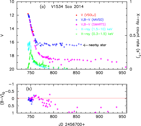
Figure 12: Optical light curve (a) and color curve (b) of V1534 Sco: (a) A few $V$ data in the very early phase are taken from VSOLJ (filled red circles). The $BV$ data are taken from AAVSO (open blue circles) and SMARTS (filled magenta stars). The AAVSO $V$ data saturate at $V\sim 16.3$ owing to contamination of a nearby star. The soft ($0.3-1.5$ keV, denoted by green crosses) and hard ($1.5-10$ keV, denoted by cyan pluses) X-ray count rates are also plotted, the data for which are taken from the Swift web site (Evans et al., 2009). (b) The $(B-V)_{0}$ are dereddened with $E(B-V)=0.93$.

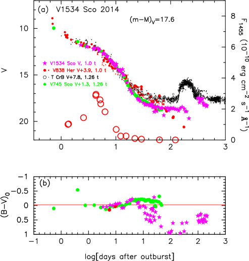
Figure 13: Same as Figure 9, but we plot the light/color curves of V1534 Sco as well as V838 Her, T CrB, and V745 Sco. (a) The filled magenta stars denote the $V$ magnitudes of V1534 Sco, the filled red circles (red dots) represent the $V$ (visual) magnitudes of V838 Her, the black open circles (black dots) indicate the $V$ (visual) magnitude of T CrB, and the filled green circles represent the $V$ magnitude of V745 Sco. (b) The $(B-V)_{0}$ colors of V1534 Sco are dereddened with $E(B-V)=0.93$.

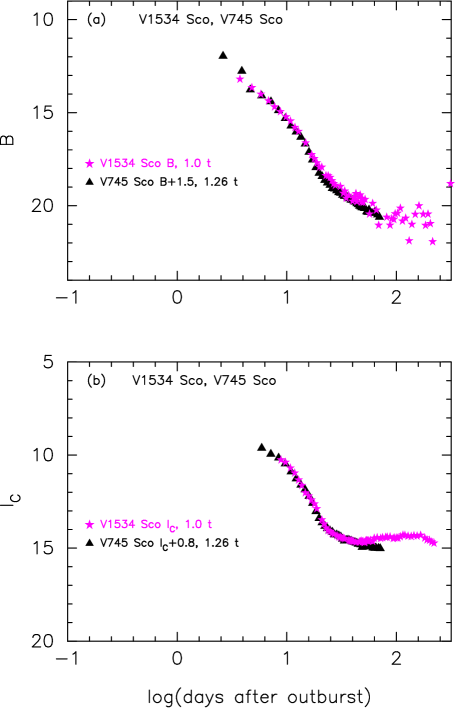
Figure 14: The (a) $B$ and (b) $I_{C}$ light curves of V1534 Sco and V745 Sco. The filled magenta stars denote the $B$ and $I_{C}$ magnitudes of V1534 Sco while the filled black triangles represent the $B$ and $I_{C}$ magnitudes of V745 Sco. The light curve of V745 Sco is stretched by $f_{\rm s}=1.26$ and shifted down by $\Delta B=1.5$ and $\Delta I_{C}=0.8$, as listed in the figure.

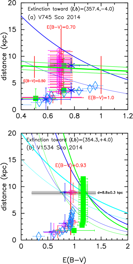
Figure 15: Distance-reddening relation toward (a) V745 Sco and (b) V1534 Sco. Each symbol and lines are the same as those in Figure 4(a) and (d), respectively. However, we plot various distance-reddening relations assuming different reddenings of $E(B-V)=1.0$ (thick solid lines) and $E(B-V)=0.5$ (thin solid lines) for V745 Sco for comparison. In panel (a), the thick/thin solid blue lines denote $(m-M)_{V}=17.5$/16.1, which are just calculated from Equation (5) together with $d=7.5$/8.1 kpc and $E(B-V)=1.0$/0.5, not a result of fitting. In panel (b), the thick/thin solid green, blue, and cyan lines denote $(m-M)_{B}=19.75$/17.85, $(m-M)_{V}=18.5$/17.1, and $(m-M)_{I}=16.5$/15.9, respectively. These three lines do not exactly but broadly cross at $d=8.5$/9.1 kpc and $E(B-V)=1.24$/0.74, respectively. See the text for detail.

2.4 V1534 Sco 2014

V1534 Sco is a classical nova in a symbiotic system (Joshi et al., 2015). Figure 12 shows (a) the $V$ and X-ray fluxes and (b) $(B-V)_{0}$ color evolutions of V1534 Sco. Here, $(B-V)_{0}$ are dereddened with $E(B-V)=0.93$ as explained below. V1534 Sco reached $m_{V,\rm max}=11.8$ on JD 2456744.27 (UT 2014 March 27.77) from the data of the Variable Star Observers League of Japan (VSOLJ). The AAVSO $V$ data becomes flat when the $V$ goes down to $V\sim 16.3$. This is an artifact due to the $V$ flux being contaminated by nearby stars (e.g., Munari et al., 2017). Therefore, we use only the data of SMARTS (Walter et al., 2012) in the following analysis. The nova declined with $t_{2}=6\pm 0.3$ day and was identified as a He/N nova by Joshi et al. (2015). Joshi et al. (2015) also obtained the reddening of $E(B-V)=0.91$ from the empirical relations derived by van den Bergh & Younger (1987), i.e., the intrinsic color of $(\bv)_{0}=0.23\pm 0.06$ at maximum and $(\bv)_{0}=-0.02\pm 0.04$ at time $t_{2}$. From the NIR spectra of this nova, Joshi et al. (2015) concluded that the nova outbursted in a symbiotic system with an M5III ($\pm$ two subclasses) RG companion and suggested that V1534 Sco is a recurrent nova such as T CrB, RS Oph, and V745 Sco. They estimated the distance to the nova as 8.1, 9.6, 13.0, 18.6, and 26.4 kpc depending on the subclass, M3III, M4III, M5III, M6III, and M7III, respectively.

2.4.1 Timescaling law and time-stretching method

Figure 13 shows the $V$ light and $(B-V)_{0}$ color curves of V1534 Sco on a logarithmic timescale. We add the light/color curves of the symbiotic recurrent novae V745 Sco and T CrB and the very fast nova V838 Her. The $V$ light curves of four novae overlap each other, i.e., Equation (10) is satisfied. Here, we determine the horizontal shift of the V745 Sco $V$ light curve with respect to V1534 Sco as $\Delta\log t=\log f_{\rm s}=0.10$. The positions of the other two novae are uniquely determined from Figure 9.

We found no reliable distance or distance modulus to V1534 Sco in the literature. Therefore, we apply Equation (11) to Figure 13 and obtain the distance modulus in the $V$ band relative to the three novae as

$$(m - M)_{V,\rm V1534~{}Sco}$$ (17)

$$= (m-M+\Delta V)_{V,\rm V745~{}Sco}-2.5\log 1.26$$ (18)

$$= 16.6\pm 0.2+1.3\pm 0.1-0.25=17.55\pm 0.2$$ (19)

$$= (m-M+\Delta V)_{V,\rm T~{}CrB}-2.5\log 1.26$$ (20)

$$= 10.1\pm 0.3+7.8\pm 0.1-0.25=17.55\pm 0.3$$ (21)

$$= (m-M+\Delta V)_{V,\rm V838~{}Her}-2.5\log 1.0$$ (22)

$$= 13.7\pm 0.3+3.9\pm 0.1-0.0=17.6\pm 0.3,$$ (23)

where we adopt $(m-M)_{V,\rm V745~{}Sco}=16.6\pm 0.2$ in Section 2.1, $(m-M)_{V,\rm T~{}CrB}=10.1\pm 0.3$ in Section 2.2, and $(m-M)_{V,\rm V838~{}Her}=13.7\pm 0.3$ in Section 2.3. Thus, we obtain $(m-M)_{V}=17.6\pm 0.3$ and $f_{\rm s}=1.26$ (against V745 Sco) for V1534 Sco.

Figure 14 shows the (a) $B$ and (b) $I_{C}$ magnitudes of V1534 Sco and V745 Sco on a logarithmic timescale. These two nova light curves overlap to each other. Therefore, we again apply Equation (11) to the $B$ magnitudes of V1534 Sco and V745 Sco in Figure 14(a), and obtain

$$(m - M)_{B,\rm V1534~{}Sco}$$ (24)

$$= (m-M+\Delta B)_{B,\rm V745~{}Sco}-2.5\log 1.26$$ (25)

$$= 17.3\pm 0.2+1.5\pm 0.1-0.25=18.55\pm 0.2,$$ (26)

where we adopt the absorption law of $A_{B}=4.1\times E(B-V)$ from Rieke & Lebofsky (1985) and use the distance-reddening relation of

$$(m-M)_{B}=4.1\times E(B-V)+5\log(d/10~{}{\rm pc}),$$ (27)

and $(m-M)_{B,\rm V745~{}Sco}=16.6+1.0\times 0.7=17.3$. Thus, we obtain $(m-M)_{B}=18.55\pm 0.2$ for V1534 Sco.

We further apply Equation (11) to the $I_{C}$ magnitudes of V1534 Sco and V745 Sco in Figure 14(b), and obtain

$$(m - M)_{I,\rm V1534~{}Sco}$$ (28)

$$= (m-M+\Delta I_{C})_{I,\rm V745~{}Sco}-2.5\log 1.26$$ (29)

$$= 15.55\pm 0.2+0.8\pm 0.1-0.25=16.1\pm 0.2,$$ (30)

where we adopt the absorption law of $A_{I}=1.5\times E(B-V)$ from Rieke & Lebofsky (1985) and use the distance-reddening relation of

$$(m-M)_{I}=1.5\times E(B-V)+5\log(d/10~{}{\rm pc}),$$ (31)

and $(m-M)_{I,\rm V745~{}Sco}=16.6-1.6\times 0.7=15.55$. Thus, we obtain $(m-M)_{I}=16.1\pm 0.2$ for V1534 Sco.

We plot the distance-reddening relations of Equations (27), (5), and (31) for $(m-M)_{B}=18.55$ (green line), $(m-M)_{V}=17.6$ (blue line), and $(m-M)_{I}=16.1$ (cyan line) for V1534 Sco in Figure 4(d). These three lines consistently cross at $d=8.8$ kpc and $E(B-V)=0.93$. This demonstrates an independent consistency check of our distance and reddening even if we assume the time-stretching method.

2.4.2 Reddening and distance

We examine this result of $(m-M)_{V}=17.6$ and $E(B-V)=0.93$ from various points of view. For the reddening toward V1534 Sco, whose galactic coordinates are $(l,b)=(354\fdg 3345,+3\fdg 9915)$, the NASA/IPAC Galactic dust absorption map gives $E(B-V)=0.93\pm 0.05$. This value is close to the value of $E(B-V)=0.91$ given by Joshi et al. (2015) and consistent with our cross point of $d=8.8$ kpc and $E(B-V)=0.93$. Therefore, we adopt $E(B-V)=0.93$ and further examine whether this value is reasonable or not.

Figure 4(d) shows various distance-reddening relations toward V1534 Sco. The vertical solid red line denotes the reddening of $E(B-V)=0.93$. The solid green, blue, and cyan lines denote the distance moduli in the $B$, $V$, and $I_{C}$ bands, i.e., $(m-M)_{B}=18.55$, $(m-M)_{V}=17.6$, and $(m-M)_{I}=16.1$. These four lines cross at $E(B-V)=0.93$ and $d=8.8$ kpc. The relations of Marshall et al. (2006) are plotted in four directions close to the direction of V1534 Sco: $(l,b)=(354\fdg 25,+3\fdg 75)$ (open red squares), $(354\fdg 50,+3\fdg 75)$ (filled green squares), $(354\fdg 25,+4\fdg 00)$ (blue asterisks), and $(354\fdg 50,+4\fdg 00)$ (open magenta circles). The direction of V1534 Sco is midway between those of the blue asterisks and open magenta circles. The open cyan-blue diamonds show the relation of Özdörmez et al. (2016), which is roughly consistent with that of Marshall et al. until $d=6$ kpc. The cross point at $E(B-V)=0.93$ and $d=8.8$ kpc is consistent with the relation of Marshall et al. Then, the vertical distance from the galactic plane is approximately $z=+610$ pc. Thus, it is likely that V1534 Sco belongs to the galactic bulge (Munari et al., 2017).

2.4.3 Color-magnitude diagram

Using $E(B-V)=0.93$ and $(m-M)_{V}=17.6$ ($d=8.8$ kpc), we plot the color-magnitude diagram of V1534 Sco in Figure 6(b). The track of V1534 Sco (filled red circles) is located closely to that of V745 Sco (open magenta diamonds). These two tracks almost overlap apart from the difference in the peak brightness: V1534 Sco has $M_{V,\rm max}=11.8-17.6=-5.8$, whereas V745 Sco reached $M_{V,\rm max}=8.66-16.6=-7.94$. This overlap supports our derived values of $E(B-V)=0.93$ and $(m-M)_{V}=17.6$ ($d=8.8$ kpc). We conclude that the distance of $d=8.8\pm 0.9$ kpc and the reddening of $E(B-V)=0.93\pm 0.05$ are reasonable. Thus, we confirm that Equations (10) and (11) are satisfied for V1534 Sco.

2.4.4 Consistency check with V745 Sco

The three relations, i.e., $(m-M)_{B}=18.55$, $(m-M)_{V}=17.6$, and $(m-M)_{I}=16.1$ for V1534 Sco, consistently cross at the point of $d=8.8$ kpc and $E(B-V)=0.93$ in the distance-reddening relation in Figure 4(d). These three distance moduli are calculated from Equations (26), (23), and (30) using V745 Sco’s $(m-M)_{B}=17.3$, $(m-M)_{V}=16.6$, and $(m-M)_{I}=15.55$. However, these V745 Sco’s values are calculated assuming the reddening of $E(B-V)=0.70$. We check the dependency on the reddening of V745 Sco.

If we adopt a different value, for example, $E(B-V)=1.0$, we have a different cross point as shown in Figure 15(a). Here we assume $(m-M)_{K}=8.33-(-6.39)=14.72$ (only this value is fixed from Equation (3) and $m_{K}=8.33$). Then, we calculate distance modulus in each band as $(m-M)_{B}=(m-M)_{K}+3.75\times E(B-V)=18.5$, $(m-M)_{V}=(m-M)_{K}+2.75\times E(B-V)=17.5$, and $(m-M)_{I}=(m-M)_{K}+1.15\times E(B-V)=15.9$ for V745 Sco. Using these different values in Equations (26), (23), and (30), we obtain $(m-M)_{B}=19.75$, $(m-M)_{V}=18.5$, and $(m-M)_{I}=16.5$ for V1534 Sco. These new three lines do not exactly but broadly cross at $d=8.5$ kpc and $E(B-V)=1.24$ as plotted (thick solid lines) in Figure 15(b). This reddening of $E(B-V)=1.24$ is much larger than the reddening of $E(B-V)=0.91$ obtained by Joshi et al. (2015) (or $E(B-V)=0.93$ of our cross point in Figure 4(d)).

Similarly if we adopt a smaller reddening of $E(B-V)=0.50$ for V745 Sco, we obtain $(m-M)_{B}=(m-M)_{K}+3.75\times E(B-V)=16.6$, $(m-M)_{V}=(m-M)_{K}+2.75\times E(B-V)=16.1$, and $(m-M)_{I}=(m-M)_{K}+1.15\times E(B-V)=15.3$ for V745 Sco. Then, we obtain $(m-M)_{B}=17.85$, $(m-M)_{V}=17.1$, and $(m-M)_{I}=15.9$ for V1534 Sco. These three lines roughly cross at $d=9.1$ kpc and $E(B-V)=0.74$ as plotted (thin solid lines) in Figure 15(b). This value of $E(B-V)=0.74$ is much smaller than $E(B-V)\approx 0.9$. Therefore, such a smaller value of $E(B-V)=0.50$ for V745 Sco is not supported.

We have already discussed the distance and reddening in Sections 2.4.2 and 2.4.3, and concluded that the reddening of $E(B-V)=0.93$ is reasonable for V1534 Sco. In other words, only the reddening of $E(B-V)\approx 0.7$ for V745 Sco is consistent with the reddening of $E(B-V)\approx 0.9$ for V1534 Sco. We should also note that the distance of V1534 Sco is well constrained to $d=8.8\pm 0.3$ kpc even for a wide range of $E(B-V)=0.5-1.0$ for V745 Sco. This analysis confirms that only the two sets of $d=7.8$ kpc and $E(B-V)=0.70$ for V745 Sco and $d=8.8$ kpc and $E(B-V)=0.93$ for V1534 Sco are consistent with each other in the distance-reddening relations and color-magnitude diagram.

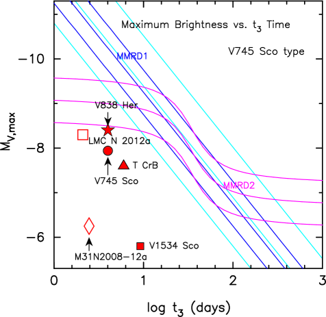
Figure 16: Maximum magnitude vs. rate of decline relations for the rapid-decline (V745 Sco) type novae. Each symbol is labeled with a nova name. The filled symbols correspond to novae in our galaxy, whereas the open symbols denote novae in extra-galaxies. Kaler-Schmidt’s law (labeled “MMRD1,” Schmidt, 1957) is denoted by a blue line with two attendant lines corresponding to the cases of $\pm 0.5$ mag brighter/fainter. Della Valle & Livio’s law (labeled “MMRD2,” della Valle & Livio, 1995) is indicated by a magenta line flanked with $\pm 0.5$ mag brighter/fainter lines. The three cyan lines represent Equations (B8), (B6), and (B10) in Appendix B, from upper to lower. These cyan lines envelop the galactic novae studied by Downes & Duerbeck (2000), as shown in Figure 51 of Appendix B. We call this region the broad MMRD relation.

2.5 Faint locations much below the MMRD relations

It has been frequently discussed that very fast novae and recurrent novae sometimes deviate from the MMRD relations (e.g., Schaefer, 2010; Hachisu & Kato, 2010, 2015, 2016a). Here, the two empirical MMRD relations are defined as (Kaler-Schmidt’s law, MMRD1)

$$M_{V,{\rm max}}=-11.75+2.5\log t_{3},$$ (32)

by Schmidt (1957), and as (Della Valle & Livio’s law, MMRD2)

$$M_{V,{\rm max}}=-7.92-0.81\arctan\left({{1.32-\log t_{2}}\over{0.23}}\right),$$ (33)

by della Valle & Livio (1995), where $M_{V,{\rm max}}$ is the absolute $V$ magnitude at maximum, ($t_{2}$ or) $t_{3}$ is the period of days during which the nova decays by (two or) three magnitudes from the $V$ maximum. We use $t_{2}\approx 0.6\times t_{3}$ (Hachisu & Kato, 2006) to calculate $t_{2}$ from $t_{3}$ in Equation (33). Kaler-Schmidt’s law is denoted in Figure 16 by a blue solid line with two attendant blue solid lines, corresponding to $\pm 0.5$ mag brighter/fainter cases. Della Valle & Livio’s law is indicated by a magenta solid line flanked with $\pm 0.5$ mag brighter/fainter cases.

As mentioned in Section 1, Hachisu & Kato (2010) theoretically examined the MMRD law on the basis of their universal decline law. They showed that the main trend of the MMRD relation is governed by the WD mass (timescaling factor of $f_{\rm s}$) and the second parameter (the initial envelope mass, i.e., the ignition mass) causes large scatter around the main trend of the MMRD relations. Hachisu & Kato (2010) reproduced the distribution of MMRD points summarized by Downes & Duerbeck (2000). We plot Hachisu & Kato’s results with the three cyan lines in Figure 16, which represent Equations (B8), (B6), and (B10) in Appendix B, from top to bottom. These three cyan lines envelop the MMRD points studied by Downes & Duerbeck (2000) as shown in Figure 51 of Appendix B. We call this region the broad MMRD relation.

In Figure 16, we plot the MMRD points $(t_{3},M_{V,\rm max})$ of the V745 Sco (rapid-decline) type novae in our galaxy, LMC, and M31, some of which (filled symbols) are discussed in this section and the others (open symbols) are examined in Section 5. They are tabulated in Table 2. All of them are far outside the broad MMRD relation (solid cyan lines). It is clear that the MMRD relations cannot be applied to the rapid-decline type novae.

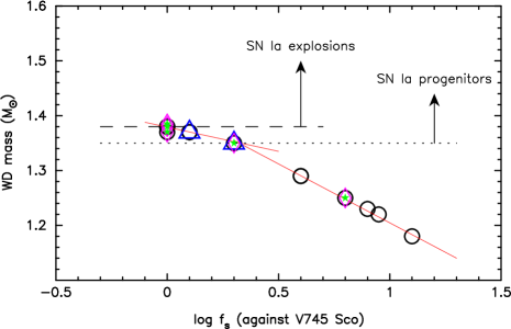
Figure 17: WD mass vs. timescaling factor $\log f_{\rm s}$. The timescaling factor is measured against that of V745 Sco ($f_{\rm s}=1.0$ for V745 Sco). The data are taken from Table 3. See the text for more detail.

2.6 WD mass vs. timescaling factor

Figure 17 shows the WD mass against the timescaling factor of $\log f_{\rm s}$, where the timescaling factor is measured based on that of V745 Sco ($f_{\rm s}=1.0$ for V745 Sco). The WD mass of V745 Sco ($\log f_{\rm s}=0.0$) is estimated to be $M_{\rm WD}=1.385~{}M_{\sun}$ from the X-ray model light curve fitting in Section 2.1. The WD mass of M31N 2008-12a ($\log f_{\rm s}=0.0$) was suggested to be $M_{\rm WD}=1.38~{}M_{\sun}$ from the X-ray and optical model light curve fitting (Kato et al., 2017, see also Section 5.6 below). The WD mass of V838 Her ($\log f_{\rm s}=0.1$) is obtained to be $M_{\rm WD}=1.37~{}M_{\sun}$ from the $V$ and UV 1455 Å model light curve fitting in Section 2.3. We plot these WD masses with open blue triangles (UV 1455 Å), open magenta diamonds ($t_{\rm SSS-on}$), and filled green stars ($t_{\rm SSS-off}$), as listed in Table 3.

Assuming that the WD mass is linearly related to the timescaling factor of $\log f_{\rm s}$ between $\log f_{\rm s}=0.0$ and $\log f_{\rm s}=0.3$ (and differently related between $\log f_{\rm s}=0.3$ and $\log f_{\rm s}=1.1$), we determine each WD mass of the novae (large open black circles) as shown in Figure 17. We estimate the ambiguity of the WD mass determination could be $\pm(0.01-0.02)~{}M_{\sun}$ from this linear relation. The main reason is the difference in the chemical composition of hydrogen-rich envelope as shown in the case of V838 Her ($1.37~{}M_{\sun}$ vs. $1.35~{}M_{\sun}$).

Among these 14 novae, we have already analyzed 4 novae in this section, i.e., T CrB ($\log f_{\rm s}=0.0$, $1.38~{}M_{\sun}$, RG, $P_{\rm orb}=227.6$ days), V838 Her ($\log f_{\rm s}=0.1$, $1.37~{}M_{\sun}$, MS, $P_{\rm orb}=0.2976$ days), V745 Sco ($\log f_{\rm s}=0.0$, $1.385~{}M_{\sun}$, RG, $P_{\rm orb}=$unknown), and V1534 Sco ($\log f_{\rm s}=0.1$, $1.37~{}M_{\sun}$, RG, $P_{\rm orb}=$unknown). It is unlikely that these WDs were born as massive as they are ($\gtrsim 1.37~{}M_{\sun}$, see, e.g., Doherty et al., 2015). We suppose that these WDs have grown in mass. This strongly suggests further increases in the WD masses in these systems.

The WD masses of SN Ia progenitors should be close to or exceed the SN Ia explosion mass of $M_{\rm Ia}=1.38~{}M_{\sun}$ (Nomoto, 1982), as mentioned in Section 1. The typical mass-increasing rates of WDs are $\dot{M}_{\rm WD}\sim 1\times 10^{-7}~{}M_{\sun}$ yr^-1 just below the stability line of hydrogen shell burning, that is, in relatively short-recurrence-period novae (see, e.g., Kato et al., 2017). The WD mass increases from $1.37~{}M_{\sun}$ to $M_{\rm Ia}=1.38~{}M_{\sun}$ and explodes as a SN Ia. It takes approximately $t_{\rm Ia}\sim 0.01~{}M_{\sun}/1\times 10^{-7}~{}M_{\sun}$ yr${}^{-1}=1\times 10^{5}$ yr, which is much shorter than the evolution timescale of the donor (RG star or MS star). Therefore, these WDs have grown in mass and will explode as a SN Ia if the core consists of carbon and oxygen.

Note that V838 Her is identified as a neon nova because the ejecta are enriched by neon. The neon rich ejecta, however, do not always mean that the underling WD has an oxygen-neon core. A mass-increasing WD, like in some recurrent novae, develops a helium layer underneath the hydrogen burning zone and experiences periodic helium shell flashes (e.g., Wu et al., 2017; Kato et al., 2017). Helium burning produces neon and other heavy elements that remain after the helium shell flash and mixed into the freshly accreted hydrogen-rich matter. The next recurrent nova outburst could show strong neon lines. Thus, the neon nova identification should not be directly connected to an oxygen-neon core when the WD mass is close to the Chandrasekhar mass. Considering this possibility and unlikely born massive WD, we regard V838 Her is a candidate of SN Ia progenitors.

2.7 Summary of the rapid-decline (V745 Sco) type novae

We summarize the results on the four rapid-decline type novae.

1. We analyzed four very fast novae including two recurrent novae, V745 Sco, T CrB, V838 Her, and V1534 Sco. We obtained the distances, distance moduli in the $V$ band, and reddenings of the four novae using various methods. The results are summarized in Table 1. These novae are located significantly above or below the scale height of galactic matter distribution ($z=\pm 125$ pc, see, e.g., Marshall et al., 2006).

2. The $V$ light curves of the four novae almost overlap when we properly stretch their timescales by a factor of $f_{\rm s}$ and shift up or down their $V$ light curves by $\Delta V$ (see Figure 2). This means that these novae satisfy the timescaling law of Equation (10). Utilizing the obtained distance moduli in the $V$ band and the time-stretching factor of $f_{\rm s}$, we confirm that these four novae satisfy the time-stretching method of Equation (11). The time-stretching method is applicable to the rapid-decline type novae including recurrent novae.

3. All the four novae are substantially fainter than the MMRD relations. In particular, V1534 Sco is located significantly below Kaler-Schmidt’s law (MMRD1) and Della Valle & Livio’s law (MMRD2). This means that the MMRD relations cannot be applied to the rapid-decline type novae.

4. The WD mass of V745 Sco is estimated to be $M_{\rm WD}=1.385~{}M_{\sun}$ from our model light curve fitting with the supersoft X-ray light curve. This WD mass is more massive than $M_{\rm WD}=1.38~{}M_{\sun}$ of the 1-yr recurrence period nova, M31N 2008-12a. This is consistent with the earlier appearance of the SSS phase of V745 Sco ($t_{\rm SSS-on}\sim 4$ days) than that of M31N 2008-12a ($t_{\rm SSS-on}\sim 6$ days).

5. The WD mass of V838 Her is independently estimated to be $M_{\rm WD}=1.37~{}M_{\sun}$ from our model light curve fitting with the UV 1455 Å light curve. This is consistent with the timescaling factor $f_{\rm s}=1.26$ of V838 Her, which is slightly longer than $f_{\rm s}=1.0$ of V745 Sco ($M_{\rm WD}=1.385~{}M_{\sun}$), suggesting that its WD mass is smaller than that of V745 Sco.

6. The rapid-decline type novae have a timescaling factor of $f_{\rm s}=1.0$ and $f_{\rm s}=1.26$. Therefore, their WD masses are $M_{\rm WD}=1.38~{}M_{\sun}$ (or $1.385~{}M_{\sun}$) and $M_{\rm WD}=1.37~{}M_{\sun}$, respectively. It is unlikely that the WDs were born as massive as they are. These WDs should have grown in mass after they were born. This supports that the rapid-decline type novae are immediate progenitors of SNe Ia if their WDs have a carbon-oxygen core.

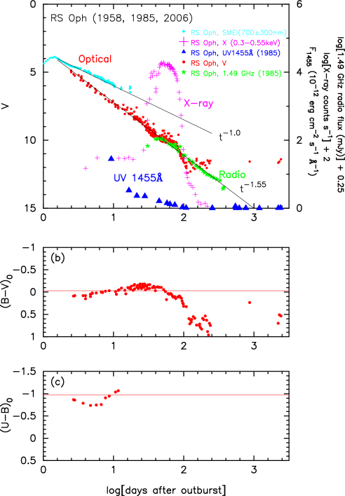
Figure 18: Same as Figure 3, but for the RS Oph 1958, 1985, and 2006 outbursts. The colors are dereddened with $E(B-V)=0.65$. (a) The $V$ data (filled red circles) are taken from Siviero & Munari (2006), AAVSO, and SMARTS for the 2006 outburst and from Connelley & Sandage (1958) for the 1958 outburst. The SMEI band data (filled cyan circles) are from Hounsell et al. (2010) for the 2006 outburst. We also plot the supersoft X-ray ($0.3-0.55$ keV, magenta plus, Hachisu et al., 2007) for the 2006 outburst, UV 1455 Å  band (filled blue triangles, Cassatella et al., 2002) and radio (1.49 GHz) band fluxes (filled green stars, Hjellming et al., 1986) for the 1985 outburst. (b) The $B-V$ data (filled red circles) are from Siviero & Munari (2006), AAVSO, and SMARTS for the 2006 outburst and from Connelley & Sandage (1958) for the 1958 outburst. (c) The $U-B$ data (filled red circles) are taken from Connelley & Sandage (1958) for the 1958 outburst.

3 Timescaling Law of CSM-shock Novae

We analyze the light curves of RS Oph and V407 Cyg and show that these two novae follow a timescaling law if we consider the interaction between ejecta and CSM. We call this group of novae the CSM-shock (RS Oph) type novae.

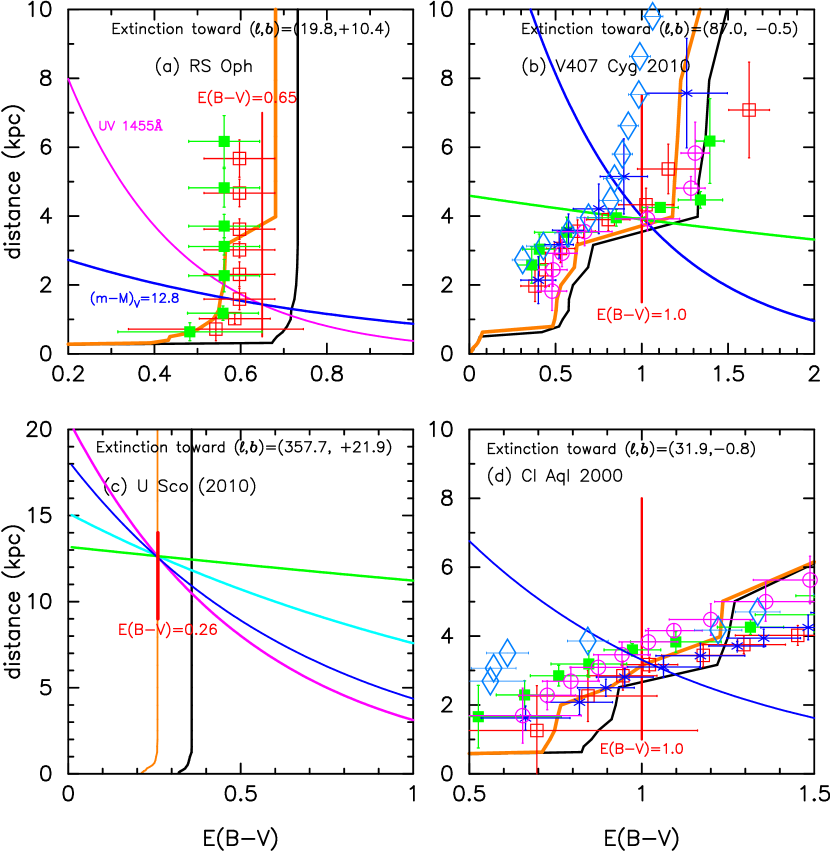
Figure 19: Same as Figure 4, but for (a) RS Oph, (b) V407 Cyg, (c) U Sco, and (d) CI Aql. The thick solid blue lines denote (a) $(m-M)_{V}=12.8$, (b) $(m-M)_{V}=16.1$, (c) $(m-M)_{V}=16.3$, and (d) $(m-M)_{V}=15.7$. In panel (c), we add three distance-reddening relations of Equations (27), (31), and (4) for U Sco, that is, $(m-M)_{B}=16.6$ (magenta line), $(m-M)_{I}=15.9$ (cyan line), and $(m-M)_{K}=15.6$ (green line).

3.1 RS Oph (2006)

RS Oph is a recurrent nova with six recorded outbursts in 1898, 1933, 1958, 1967, 1985, and 2006 (e.g., Schaefer, 2010). The orbital period of 453.6 days was obtained by Brandi et al. (2009). Figure 18 shows (a) the $V$ magnitudes, SMEI magnitudes (Hounsell et al., 2010), radio (1.49 GHz) fluxes (Hjellming et al., 1986), UV 1455 Å, and X-ray light curves, (b) $(B-V)_{0}$, and (c) $(U-B)_{0}$ color curves of RS Oph on a logarithmic timescale. The $V$ magnitude reaches $m_{V,\rm max}=4.8$ and declines with $t_{2}=6.8$ and $t_{3}=14$ days (Schaefer, 2010). The WD mass of RS Oph was estimated to be $M_{\rm WD}=1.35\pm 0.01~{}M_{\sun}$ by Hachisu et al. (2006b, 2007) from the model $V$ and supersoft X-ray light curve fittings. Thus, we regard the WD mass of RS Oph to be $1.35~{}M_{\sun}$. Hachisu & Kato (2001b) argued that RS Oph is a progenitor of SNe Ia because the WD mass is close to the SN Ia explosion mass of $M_{\rm Ia}=1.38~{}M_{\sun}$ and now increases. Mikołajewska & Shara (2017) also reached a similar conclusion.

The $V$ and radio light curves clearly show the trend of $F_{\nu}\propto t^{-1.55}$, as shown in Figure 18(a). However, the SMEI magnitude light curve has a different trend of $L_{\rm SMEI}\propto t^{-1.0}$, where $L_{\rm SMEI}$ is the luminosity of the SMEI band. This is because the SMEI magnitude is a wide-band (peak quantum efficiency at 700 nm with a full width at half maximum (FWHM) of 300 nm) and include the flux of very strong H$\alpha$ line, which mainly comes from the shock interaction. RS Oph has a RG companion and the companion star emits cool slow winds ($\sim 40$ km s^-1, see Iijima, 2009), which form CSM around the binary before the nova outburst. The ejecta of the nova outburst have high velocity, up to $\sim 4000$ km s^-1, and collide with the CSM, giving rise to strong shock (e.g., Sokoloski et al., 2006). The shock interaction contributes to the H$\alpha$ line and slows the decay of SMEI magnitude. Such an interaction between ejecta and CSM was frequently observed in supernovae Type IIn, and the relation $L_{V}\propto t^{-1.0}$ in the $V$-band luminosity was calculated by Moriya et al. (2013) for SN 2005ip. We discuss this point in more detail in the next subsection on V407 Cyg.

For the reddening and distance modulus toward RS Oph, we adopt $E(B-V)=0.65\pm 0.05$ and $(m-M)_{V}=12.8\pm 0.2$ after Hachisu & Kato (2016b). The distance is calculated to be $d=1.4\pm 0.2$ kpc. This reddening is roughly consistent with those obtained by Snijders (1987), i.e., $E(B-V)=0.73\pm 0.06$ from the He II line ratio of 1640Å  and 3203Å, and $E(B-V)=0.73\pm 0.10$ from the 2715Å interstellar dust absorption feature. The NASA/IPAC galactic dust absorption map also gives $E(B-V)=0.64\pm 0.03$ in the direction toward RS Oph, whose galactic coordinates are $(l,b)=(19\fdg 7995,+10\fdg 3721)$.

There are still debates on the distance to RS Oph (see, e.g., Schaefer, 2010). Hjellming et al. (1986) estimated the distance to be 1.6 kpc from H I absorption-line measurements. Snijders (1987) also obtained the distance of 1.6 kpc assuming the UV peak flux is equal to the Eddington luminosity. Harrison et al. (1993) calculated a distance of 1290 pc from the $K$-band luminosity. Hachisu & Kato (2001b) obtained a smaller distance of 0.6 kpc from the comparison of observed and theoretical UV fluxes integrated for the wavelength region of 911-3250 Å . They assumed blackbody radiation at the photosphere, although the free-free flux is much larger than the blackbody flux in this wavelength region. Hachisu et al. (2006b) revised the distance to be $1.3-1.7$ kpc from the $y$ and $I_{c}$ band light curve fittings in the late phase of the 2006 outburst. O’Brien et al. (2006) estimated the distance of 1.6 kpc from VLBA mapping observation with an expansion velocity indicated from emission line width. Monnier et al. (2006) estimated a shorter distance of $<540$ pc assuming that the IR interferometry size corresponds to the binary separation. If we regard this IR emission region as a circumbinary disk, we get a much larger distance. Barry et al. (2008) reviewed various estimates and summarized that, for the 2006 outburst, the canonical distance is $1.4^{+0.6}_{-0.2}$ kpc. On the other hand, Schaefer (2009) proposed $d=4.2\pm 0.9$ kpc assuming that the companion fills its Roche lobe. We do not think that this assumption is supported by observation (e.g., Mürset & Schmid, 1999). Therefore, our adopt value of $1.4\pm 0.2$ kpc is roughly consistent with many other estimates except for Schaefer’s large value.

We plot the color-magnitude diagram of RS Oph in Figure 6(c), the data of which are taken from Connelley & Sandage (1958) (filled red circles) for the 1958 outburst, and AAVSO (open red diamonds), VSOLJ (encircled magenta pluses), SMARTS (blue stars), and Sostero & Guido (2006a, b) (filled blue triangles), Sostero et al. (2006c) (filled blue triangles) for the 2006 outburst.

Figure 19(a) shows various distance-reddening relations toward RS Oph. In the figure, we plot the vertical red line of $E(B-V)=0.65$, the distance modulus in the $V$ band of $(m-M)_{V}=12.8$ (solid blue line), the UV 1455 Å flux fitting (solid magenta line), the relations of Marshall et al. (2006): $(l,b)=(19\fdg 75,+10\fdg 0)$ (open red squares) and $(l,b)=(20\fdg 0,+10\fdg 0)$ (filled green squares), and the relations of Green et al. (2015, 2018) (solid black and orange lines, respectively). The three lines of $E(B-V)=0.65$, $(m-M)_{V}=12.8$, and UV 1455 Å flux fitting consistently cross at $E(B-V)=0.65$ and $d=1.4$ kpc. Then, the location of RS Oph is approximately $z=+250$ pc above the galactic plane. These data are the same as those in Figure 15 of Hachisu & Kato (2016b). The relation of Green et al. (2015) (black line) gives a larger value of $E(B-V)=0.73$ for $d>2$ kpc. However, the NASA/IPAC galactic dust absorption map gives $E(B-V)=0.64\pm 0.03$ in the direction toward RS Oph, which is consistent with our value of $E(B-V)=0.65\pm 0.05$.

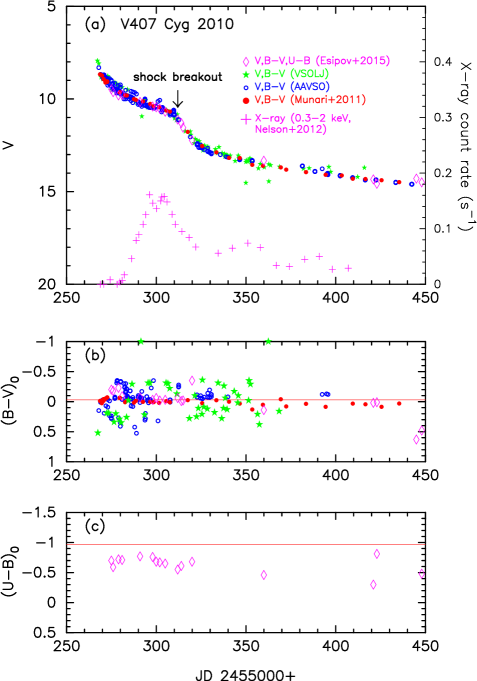
Figure 20: Same as Figure 12, but for V407 Cyg. (a) The $UBV$ data (open magenta diamonds) are taken from Esipov et al. (2015). The $BV$ data (filled green stars) are from VSOLJ. The $BV$ data (open blue circles) are from AAVSO. The $BV$ data (filled red circles) are from Munari et al. (2011b). The X-rays ($0.3-2.0$ keV, denoted by magenta pluses) are from Nelson et al. (2012). The $V$ light curve shows a sharp decay around JD 2455310, which we identify as the shock breakout. (b) The $(B-V)_{0}$ are dereddened with $E(B-V)=1.0$. (c) The $(U-B)_{0}$ are dereddened with $E(B-V)=1.0$. The horizontal solid red line denotes the color of optically thick free-free emission, i.e., $(U-B)_{0}=-0.97$.

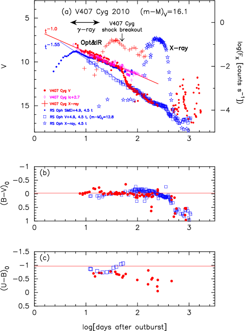
Figure 21: Same as Figure 8, but we plot the light/color curves of V407 Cyg and RS Oph. (a) The filled red circles denote the $V$ magnitudes of V407 Cyg, and the open blue squares represent the $V$ magnitudes of RS Oph. The $V$ data of V407 Cyg are taken from Munari et al. (2011b) and Esipov et al. (2015). We add the $I_{C}$ magnitudes (open magenta diamonds taken from AAVSO and VSOLJ) of V407 Cyg and the SMEI magnitudes (filled blue circles) of RS Oph. We also add the X-ray fluxes of V407 Cyg (red pluses) and RS Oph (open blue stars). The (b) $(B-V)_{0}$ and (c) $(U-B)_{0}$ color curves. The $(B-V)_{0}$ and $(U-B)_{0}$ are dereddened with $E(B-V)=1.0$ and $E(B-V)=0.65$ for V407 Cyg and RS Oph, respectively. See the text for more detail.

3.2 V407 Cyg 2010

V407 Cyg is a well-observed symbiotic nova (e.g., Munari et al., 1990), in which a WD accretes mass from a cool RG companion via the Roche-lobe overflow or stellar wind. The RG companion of V407 Cyg is a Mira with the pulsation period of 762.9 days in the $K$ band (Kolotilov et al., 2003). SiO maser observations suggest that the Mira companion has already reached a very late evolution stage of an AGB star (Deguchi et al., 2011; Cho et al., 2015). The 2010 outburst of V407 Cyg was discovered on UT 2010 March 10.813 at $m_{V}=7.6$ (Nishiyama et al., 2010). Figure 20 shows (a) the $V$ and X-ray light curves, (b) $(B-V)_{0}$, and (c) $(U-B)_{0}$ color curves of V407 Cyg. Here, $(B-V)_{0}$ and $(U-B)_{0}$ are dereddened with $E(B-V)=1.0$, as explained below. The nova reached $m_{V,\rm max}=7.1$ on UT 2010 March 10.8 (JD 2455266.3) and then declined with $t_{2}=5.9$ days and $t_{3}=24$ days in the $V$-band (Munari et al., 2011b). The $V$ light curve sharply drops around JD 2455310.

X-rays were observed with Swift, which are interpreted in terms of strong shock heating between the ejecta and circumstellar cool wind (Nelson et al., 2012). The strong shock possibly produced gamma-rays by accelerating high-energy particles. V407 Cyg is the first gamma-ray-detected nova with Fermi/Large Area Telescope (LAT) (Abdo et al., 2010). Since V407 Cyg, gamma-rays were observed in six novae between 2010 and 2015, i.e., V1324 Sco, V959 Mon, V339 Del, V1369 Cen, V745 Sco, and V5668 Sgr (e.g., Ackermann et al., 2014; Morris et al., 2017).

3.2.1 Reddening

Many authors adopted the reddening of $E(B-V)=0.57$ and the distance of $d=2.7$ kpc after Munari et al. (1990), who derived $E(B-V)=0.57$ by fitting the broad-band spectrum of V407 Cyg with an M6III model spectrum and $d=2.7$ kpc from the Mira period-luminosity relation. Shore et al. (2011) derived $E(B-V)=0.45\pm 0.05$ from the depth of the diffuse interstellar absorption bands and proposed that the Mira looks like an M8III rather than M6III type. Iijima (2015) argued that the diffuse interstellar bands cannot give a reliable reddening because the different bands resulted in very different values of the reddening; for example, $E(B-V)=0.15$ from the band at $\lambda=6613$ Å but $E(B-V)=0.76$ from the band at $\lambda=6270$ Å of his spectra. Iijima (2015) obtained $E(B-V)=0.6$ from the color excess relation of $E(B-V)=(B-V)-(B-V)_{0}$ and the empirical relation of the intrinsic color of $(\bv)_{0}=-0.02\pm 0.04$ at time $t_{2}$ (van den Bergh & Younger, 1987). He used the $B-V$ colors of VSOLJ/VSNET which are rather scattered and not reliable, as clearly shown in Figure 20(b). If we use the $B-V$ colors of Munari et al. (2011b), i.e., the filled red circles in Figure 20(b), the empirical relation of van den Bergh & Younger (1987) gives a reddening value of $E(B-V)\sim 1.0$ at $t_{2}$-time. In the present study, we adopt $E(B-V)=1.0$ which is examined in detail in Sections 3.2.2, 3.2.6, and 3.2.7.

3.2.2 Distance-reddening relation

V407 Cyg is a symbiotic binary star system consisting of a mass-accreting hot WD and a cool Mira giant with a pulsation period of 762.9 days in the $K$ band (Kolotilov et al., 2003). The period-luminosity relation of the LMC Miras has a bend at the pulsation period of $\sim 400$ days (Ita & Matsunaga, 2011). Beyond the bend, Ita & Matsunaga (2011) obtained the period-luminosity relation as

$$M_{K_{\rm s}}=(-6.850\pm 0.901)\log P+28.225\pm 2.493-\mu_{0,\rm LMC},$$ (34)

where $P(>400$ days) is the pulsation period in days and $\mu_{0,\rm LMC}$ is the distance modulus toward LMC. We adopt $\mu_{0,\rm LMC}=18.493\pm 0.048$ (Pietrzyński et al., 2013). Substituting $P=762.9$ days into Equation (34), we obtain the absolute $K_{\rm s}$ magnitude of $M_{K_{\rm s}}=-10.01$. The average $K$ mag of V407 Cyg is $m_{K}=3.3$, and thus we have

$$(m-M)_{K}=0.353\times E(B-V)+5\log(d/1{\rm~{}kpc})+10=13.31,$$ (35)

where we adopt the reddening law of $A_{K}=0.353\times E(B-V)$ (Cardelli et al., 1989). We plot this distance-reddening relation of $(m-M)_{K}=13.31$ using the thick green line in Figure 19(b). Substituting $E(B-V)=1.0$ into Equation (35), we obtain the distance of $d=3.9$ kpc. Then, the location of V407 Cyg is $z=-33$ pc below the galactic plane, because the galactic coordinates of V407 Cyg are $(l,b)=(86\fdg 9826,-0\fdg 4820)$. The distance modulus in the $V$ band is calculated to be $(m-M)_{V}=16.1$ from Equation (5). In the same figure, we include the distance-reddening law of $(m-M)_{V}=16.1$ (solid blue line) and the reddening of $E(B-V)=1.0$ (vertical solid red line).

Figure 19(b) also shows various 3D extinction maps toward V407 Cyg. The relations of Marshall et al. (2006) are plotted in four directions close to the direction of V407 Cyg: $(l,b)=(86\fdg 75,-0\fdg 25)$ (open red squares), $(87\fdg 00,-0\fdg 25)$ (filled green squares), $(86\fdg 75,-0\fdg 50)$ (blue asterisks), and $(87\fdg 00,-0\fdg 50)$ (open magenta circles). The closest one is that of the open magenta circles. We include the relations of Green et al. (2015, 2018) (thick solid black and orange lines, respectively) and Özdörmez et al. (2016) (open cyan-blue diamonds). The 3D distance-reddening relations of Marshall et al. and Green et al., $(m-M)_{V}=16.1$, $(m-M)_{K}=13.31$, and $E(B-V)=1.0$ consistently cross each other at the distance of $d=3.9$ kpc (and the reddening of $E(B-V)=1.0$). Thus, we finally confirm that the reddening of $E(B-V)=1.0$ and the distance modulus in the $V$ band of $(m-M)_{V}=16.1$ are reasonable.

3.2.3 CSM-shock interaction

Figure 21(a) shows a comparison of light curves of V407 Cyg and RS Oph on a logarithmic timescale. We stretch the timescale of RS Oph by a factor of $f_{\rm s}=4.5$ and shift down both the $V$ and SMEI light curves of RS Oph by 4.9 mag. The $V$ light curve of RS Oph (open blue squares) overlaps that of V407 Cyg (filled red circles) in the later phase, whereas the SMEI light curve of RS Oph (blue dots) overlap the $V$ light curve of V407 Cyg (filled red circles). The $V$ light curve of V407 Cyg decays as $F_{\nu}\propto t^{\alpha}$ ($\alpha=-1.0$, denoted by the solid red line) in the early phase (up to $t\sim 45$ days).

Cool winds from the Mira companion form CSM around the binary (e.g., Mohamed & Podsiadlowski, 2012). The nova ejecta collide with the CSM and form a strong shock (e.g., Orlando & Drake, 2012; Pan et al., 2015). Shore et al. (2011) and Iijima (2015) showed that the strong shock between the ejecta and CSM contributes to the emission lines and soft X-ray flux. Such an interaction between ejecta and CSM was frequently observed in supernovae Type IIn. For example, Moriya et al. (2013) showed that $F_{\nu}\propto t^{\alpha}$ ($\alpha\approx-1.0$) in the $V$-band for SN 2005ip. Thus, we interpret this early decay of $F_{\nu}\propto t^{-1}$ as the shock interaction. The $I_{C}$ light curve of V407 Cyg also show a decline trend of $F_{\nu}\propto t^{-1.0}$, which is shifted down by 2.7 mag.

Considering the shock interaction, we propose the evolution of V407 Cyg $V$ light curve as follows: in the early stage, just after the optical maximum, the ejecta collide with the CSM and produce a strong shock. This shock-heating contributes significantly to the $V$ brightness. Then, the shock broke out of the CSM approximately 45 days after the outburst (JD 2455310). Soon after the shock breakout, the $V$ light curve decays as $F_{\nu}\propto t^{-1.55}$, as shown in Figure 21(a). This $\alpha=-1.55$ is close to the universal decline law of $\alpha=-1.75$ (see Hachisu & Kato, 2006).

RS Oph decays as $F_{\nu}\propto t^{-1.55}$ in the $V$ band, as shown in Figure 18(a). The CSM shock is much weaker in RS Oph than in V407 Cyg, such that the $V$ light curve of RS Oph is close to that of the universal decline law ($F_{\nu}\propto t^{-1.75}$) showing no indication of strong shock interaction ($F_{\nu}\propto t^{-1.0}$). The radio flux also follows the same decline trend of $F_{\nu}\propto t^{-1.55}$ in the later phase. In other words, the shock interaction is strong enough to increase the continuum flux to $F_{\nu}\propto t^{-1.0}$ in V407 Cyg, but not enough in RS Oph. In contrast, the SMEI light curve of RS Oph almost obeys $L_{\rm SMEI}\propto t^{-1.0}$ like the early decline trend of V407 Cyg, where $L_{\rm SMEI}$ is the SMEI band luminosity. This is because the SMEI magnitude is a wide-band (peak quantum efficiency at 700 nm with an FWHM of 300 nm) and envelopes a very strong H$\alpha$ line, which mainly comes from the shock interaction.

It should be noted that the three rapid-decline novae, V745 Sco, T CrB, and V1534 Sco, also have a RG companion but do not show clear evidence of shock-heating in their $V$ (or visual) light curves, because no part shows $F_{\nu}\propto t^{-1}$. Their $V$ light curves almost overlap to that of V838 Her, which has a MS companion as mentioned in Section 2.3. The X-ray fluxes of V407 Cyg, RS Oph, V745 Sco, and V1534 Sco were observed with Swift. Their origin could be shock-heating in the very early phase, before the SSS phase started. Munari & Banerjee (2018) showed no evidence of deceleration of ejecta in V1534 Sco. These indicate that the shape of $V$ light curve changes from that of V407 Cyg to RS Oph, and finally to V1534 Sco, depending on the strength of shock interaction. V407 Cyg shows a strongest limit of shock interaction while V1534 Sco corresponds to a weakest limit of shock.

3.2.4 Timescaling law and time-stretching method

As discussed in the previous subsection, the $V$ light curve of V407 Cyg essentially follows a similar decline law to RS Oph. We apply V407 Cyg and RS Oph to Equations (10) and (11) and obtain the following relation

$$(m - M)_{V,\rm V407~{}Cyg}=16.1$$ (36)

$$= (m-M+\Delta V)_{V,\rm RS~{}Oph}-2.5\log f_{\rm s}$$ (37)

$$= 12.8+\Delta V-2.5\log f_{\rm s},$$ (38)

where we adopt $(m-M)_{V,\rm RS~{}Oph}=12.8$ in Section 3.1. We have the relation between $\Delta V$ and $f_{\rm s}$ as

$$\Delta V-2.5\log f_{\rm s}=3.3,$$ (39)

where $\Delta V$ is the vertical shift and $\log f_{\rm s}$ is the horizontal shift with respect to the original $V$ light curve of RS Oph in Figure 18(a). If we choose an arbitrary $\Delta V$, these two $V$ light curves do not overlap. We search by eye for the best-fit value by changing $\Delta V$ in steps of $0.1$ mag and obtain the set of $\Delta V$ and $\log f_{\rm s}$ for best overlap; $\Delta V=4.9$ and $\log f_{\rm s}=0.65$ ($f_{\rm s}=4.5$), as shown in Figure 21.

3.2.5 WD mass of V407 Cyg

Using the linear relation between $M_{\rm WD}$ and $\log f_{\rm s}$ in Figure 17, we obtain the WD mass of $M_{\rm WD}=1.22~{}M_{\sun}$ for V407 Cyg (see also Table 3). Here, we use the linear relation between $\log f_{\rm s}=0.3$ and $\log f_{\rm s}=1.1$ (right solid red line). Even if we assume the WD mass increases at the rate of $\dot{M}_{\rm WD}=1\times 10^{-7}~{}M_{\sun}$ yr^-1 as discussed in Section 2.6, it takes $t_{\rm Ia}=(1.38-1.22)~{}M_{\sun}/1\times 10^{-7}M_{\sun}$ yr${}^{-1}=1.6\times 10^{6}$ yr to explode as a SN Ia. We do not expect that this high mass-accretion rate will continue for such a long time, because the Mira companion has already reached a very late evolution stage of an AGB star as suggested by the SiO maser observations (Deguchi et al., 2011; Cho et al., 2015). Therefore, we suppose that V407 Cyg is not a progenitor of SNe Ia.

3.2.6 Color-magnitude diagram

Using $E(B-V)=1.0$ and $(m-M)_{V}=16.1$, we plot the color-magnitude diagram of V407 Cyg in Figure 6(d). The color evolves down along with the red solid line of $(B-V)_{0}=-0.03$, which is the intrinsic color of optically thick winds (e.g., Hachisu & Kato, 2014). Note that the track of V407 Cyg is very similar to and closely located to that of RS Oph (Figure 6(c)). Here, we adopt only the data of Munari et al. (2011b) and Esipov et al. (2015) because the other $B-V$ color data of the VSOLJ and AAVSO archives are rather scattered, as can be seen in Figure 20(b). This similarity again confirms that our adopted values of $E(B-V)=1.0$ and $(m-M)_{V}=16.1$ ($d=3.9$ kpc) are reasonable.

3.2.7 Discussion on the distance

The distance to V407 Cyg was determined to be $d=2.7$ kpc by Munari et al. (1990) or $d=1.9$ kpc by Kolotilov et al. (1998), based on the absolute $K$ magnitudes of the Mira companion, which were calculated from the period-luminosity relation of the Mira variables (Glass & Feast, 1982; Feast et al., 1989). Munari et al. (1990) assumed $E(B-V)=0.57$, $J=5.1$, $H=4.0$, $K=3.3$, and the relations given by Glass & Feast (1982), whereas Kolotilov et al. (1998) used $E(B-V)=0.40$, $L_{\rm cool,max}=4.7\times 10^{3}L_{\sun}(d/{\rm kpc})^{2}$ from the spectral energy distribution (SED) fitting with the cool RG and $L_{\rm cool,mid}=1.2\times 10^{4}L_{\sun}$ from the period-luminosity relation of Feast et al. (1989). However, a bend was recently found at $P\sim 400$ days in the period-luminosity relation of Mira variables (e.g., Ita & Matsunaga, 2011). Above the bend, i.e., $P\gtrsim 400$ days, the intrinsic luminosity of a Mira is much brighter than the old period-luminosity relation. Iijima (2015) made his period-luminosity relation of Mira variables for $P>400$ days. Using the minimum $K$ magnitudes of V407 Cyg, he obtained the distance of $5.3\pm 1$ kpc, much larger than the old values of 2.7 and 1.9 kpc. Instead of Iijima’s relation, we adopted the period-luminosity relation obtained by Ita & Matsunaga (2011) and estimated the distance modulus in the $K$-band, i.e., $(m-M)_{K}=13.31$ (thick solid green line in Figure 19(b)). This relation gives a reasonable cross point of $E(B-V)=1.0$ and $d=3.9$ kpc with the distance modulus in the $V$-band, i.e., $(m-M)_{V}=16.1$ (solid blue line in Figure 19(b)). This cross point is consistent with the distance-reddening relation given by Marshall et al. (2006) (open magenta circles in Figure 19(b)) and by Green et al. (2015, 2018) (solid black and orange lines). This consistency supports our new estimates of $E(B-V)=1.0$ and $d=3.9$ kpc ($(m-M)_{V}=16.1$).

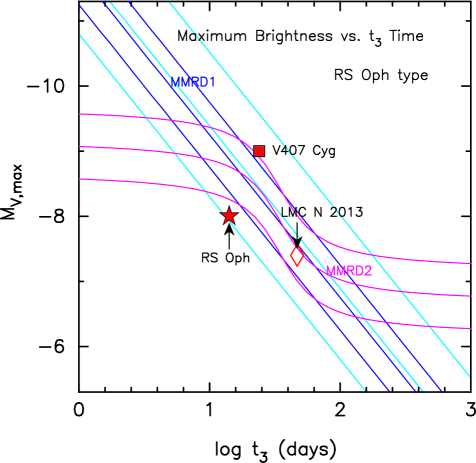
Figure 22: Same as Figure 16, but for the CSM-shock (RS Oph) type novae. The three novae, which are contaminated by shock-heating, are virtually consistent with the MMRD relations.

3.3 Template light curves of CSM-shock type novae

We have analyzed two novae, RS Oph and V407 Cyg, both of which have CSM that was shock-heated by the ejecta. The $V$ light curves of these novae were influenced by this shock-heating. The decay of optical and NIR light curves obeys the $F_{\nu}\propto t^{-1}$ (or $L_{\rm SMEI}\propto t^{-1}$ for RS Oph) during the strong deceleration phase of the ejecta. After the shock breaks out of the CSM, the decay follows $F_{\nu}\propto t^{-1.55}$, which is close to the universal decline law of $F_{\nu}\propto t^{-1.75}$. Thus, we propose the template $V$ light curves of the CSM-shock type novae, as shown in Figure 1, which are represented by, and can be applied to, both the V407 Cyg and RS Oph $V$ light curves.

The three rapid-decline novae, V745 Sco, T CrB, and V1534 Sco, have a RG companion, although they show no part of shock-heating in the $V$ light curve. We conclude that the effect of shock-heating is strongest in V407 Cyg and becomes weaker in RS Oph, V745 Sco, and V1534 Sco, in that order. V407 Cyg behaves as $F_{\nu}\propto t^{-1}$ in the early phase both of $V$ and $I_{C}$ magnitudes; RS Oph has no part of $F_{\nu}\propto t^{-1}$ in the $V$ magnitude but has a part of $F_{\nu}\propto t^{-1}$ in the SMEI magnitude, V745 Sco and V1534 Sco have no part of $F_{\nu}\propto t^{-1}$ but emit X-ray (possibly shock-origin) before the SSS phase.

3.4 MMRD relation of CSM-shock type novae

We plot each MMRD point in Figure 22 for the CSM-shock type novae. In the figure, we include another nova observed in LMC, which is analyzed in Section 5 and categorized to the CSM-shock type. It seems that these novae broadly follow both the MMRD1 (Kaler-Schmidt’s law) and MMRD2 (Della Valle & Livio’s law), although RS Oph is located slightly below the MMRD relations. The light curves of V407 Cyg and LMC N 2013 are contaminated by the flux from shock-heating and the slow decline rates make the $t_{2}$ and $t_{3}$ times longer. If we take the SMEI light curve of RS Oph, $F_{\nu}\propto t^{-1.0}$, the $t_{3}$ time becomes longer and its MMRD point is calculated to be $(t_{3},M_{V,\rm max})=($60 days, $-8.0$), which is located on the upper flanked line of the MMRD1 relation (blue line in Figure 22). Conversely, if there is no contribution from the CSM shock, V407 Cyg and LMC N 2013 should be located at the rather left side of the MMRD1 relation but still inside the cyan lines (broad MMRD region). These left-lower side positions are consistent with the general trend of normal-decline type novae which will be examined later in Section 4.

3.5 Summary of the CSM-shock (RS Oph) type novae

We summarize the results of the two CSM-shock type novae.

1. We have estimated the distance, reddening, and distance modulus of RS Oph using various methods after Hachisu & Kato (2016b). The results are summarized in Table 1.

2. We have also estimated the distance, reddening, and distance modulus of V407 Cyg using various methods, especially, from the new Mira period-luminosity relation proposed by Ita & Matsunaga (2011). The results are summarized in Table 1.

3. The $V$ light curve of V407 Cyg decays as $F_{\nu}\propto t^{-1.0}$ in the early phase (up to $t\sim 45$ days) and then sharply drops and obeys $F_{\nu}\propto t^{-1.55}$ like RS Oph after the shock breaks out of the CSM. Thus, V407 Cyg follows a timescaling law similar to RS Oph except for the early shock interaction phase.

4. We confirm that these two novae satisfy the time-stretching method, i.e., Equations (10) and (11).

5. These two novae broadly follow the MMRD relations, i.e., Kaler-Schmidt’s law (MMRD1) and the law of Della Valle & Livio (MMRD2).

6. The WD mass of RS Oph is $M_{\rm WD}=1.35~{}M_{\sun}$ and very close to the critical mass of SN Ia explosion, $M_{\rm Ia}=1.38~{}M_{\sun}$ (Nomoto, 1982). The numerical simulations show that the WD grows in mass (Hachisu & Kato, 2001b; Kato et al., 2017). This suggests that RS Oph is a progenitor of SNe Ia.

7. The WD mass of V407 Cyg is estimated to be $M_{\rm WD}=1.22~{}M_{\sun}$ from the timescaling factor of $f_{\rm s}=8.9$ against V745 Sco as listed in Table 3. SiO maser observations suggest that the Mira companion has already reached a very late evolution stage of an AGB star (Deguchi et al., 2011; Cho et al., 2015). It is unlikely that the WD mass will increase to $M_{\rm Ia}=1.38~{}M_{\sun}$ during the remaining of life of the Mira companion. Therefore, V407 Cyg is not a progenitor of SNe Ia.

4 Timescaling Law of Normal-decline Novae

We analyze the light curves of the two recurrent novae, U Sco and CI Aql, and show that they follow a timescaling law. We call this group of novae the normal-decline (U Sco) type novae.

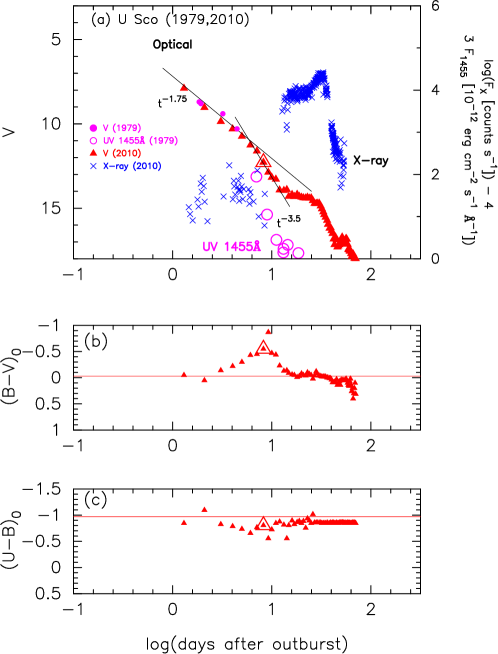
Figure 23: Light/color curves of the U Sco 1979 and 2010 outbursts. (a) The filled red triangles denote the $V$ magnitudes of the U Sco (2010) outburst, and the filled and open magenta circles represent the $V$ and UV 1455 Å fluxes of the U Sco (1979) outburst, respectively. The blue crosses are the X-ray ($0.3-10$ keV) count rates of the U Sco (2010) outburst. The (b) $(B-V)_{0}$ and (c) $(U-B)_{0}$ color curves of the U Sco (2010) outburst. The large red triangle indicates the start of the nebular phase approximately eight days after the outburst. See the text for detail.

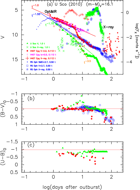
Figure 24: Same as Figure 21, but for the light/color curves of U Sco as well as RS Oph and V407 Cyg. (a) The filled green triangles denote the $V$ magnitudes of U Sco, the open blue squares represent the $V$ magnitudes of RS Oph and the filled red circles are the $V$ magnitudes of V407 Cyg. We add the X-ray count rates of U Sco (green crosses) as well as RS Oph (open blue stars) and V407 Cyg (red pluses). The blue dots are the SMEI magnitudes of RS Oph and open magenta diamonds are the $I_{C}$ magnitude of V407 Cyg. The (b) $(B-V)_{0}$ and (c) $(U-B)_{0}$ color curves.

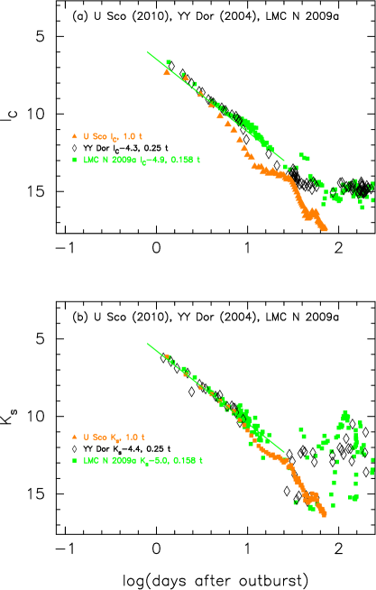
Figure 25: The (a) $I_{C}$ and (b) $K_{s}$ light curves of U Sco (2010), YY Dor (2004), and LMC N 2009a. Each light curve is horizontally stretched by $\log f_{\rm s}$ and vertically shifted by $\Delta I_{C}$ or $\Delta K_{s}$. See the text for detail.

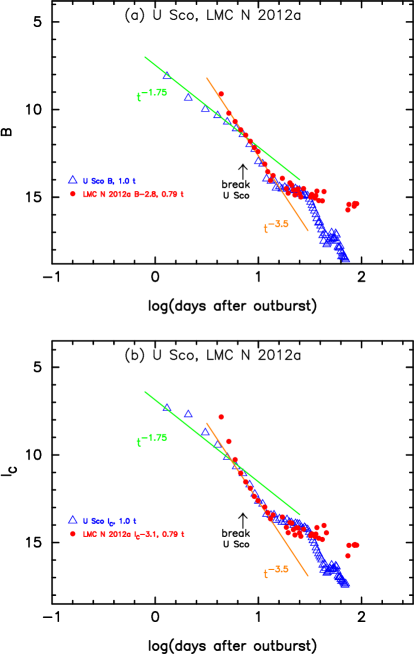
Figure 26: The (a) $B$ and (b) $I_{C}$ light curves of U Sco (2010) and LMC N 2012a. The light curves of LMC N 2012a are horizontally stretched by $\log f_{\rm s}=0.1$ and vertically shifted by $\Delta B=-2.8$ and $\Delta I_{C}=-3.1$. See the text for detail.

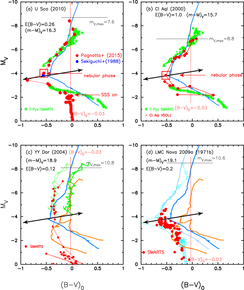
Figure 27: Same as Figure 6, but for (a) U Sco, (b) CI Aql, (c) YY Dor, and (d) LMC N 2009a. The thick solid cyan-blue lines show the template track of V1500 Cyg. The thick solid orange lines show the template track of LV Vul. The thick solid green lines show the template track of V1668 Cyg. In panels (a) and (b), we add the data of the T Pyx 2011 outburst (filled green stars, taken from SMARTS), which are the same as those in Figures 16 and 19 of Hachisu & Kato (2016b). In panel (c), the thin solid green lines correspond to the track of V1668 Cyg but blue-shifted by $\Delta(B-V)_{0}=-0.3$ mag. The track of YY Dor (filled red circles connected with a solid red line) almost overlaps with this blue-shifted V1668 Cyg track. In panel (d), the thin solid cyan-blue lines denote a $\Delta(B-V)_{0}=-0.2$ mag blue-shifted track of V1500 Cyg. The open cyan squares connected with thin solid cyan line represent a U Sco track blue-shifted by $\Delta(B-V)_{0}=-0.15$ mag.

4.1 U Sco (2010)

U Sco is a recurrent nova with ten recorded outbursts in 1863, 1906, 1917, 1936, 1945, 1969, 1979, 1987, 1999, and 2010, nearly every ten years (Schaefer, 2010). Figure 23 shows (a) the $V$, UV 1455 Å, and X-ray, (b) $(B-V)_{0}$, and (c) $(U-B)_{0}$ evolutions of the U Sco (1979, 2010) outbursts on a logarithmic timescale. Here, $(B-V)_{0}$ and $(U-B)_{0}$ of U Sco are dereddened with $E(B-V)=0.26$, as explained below. The $UBV$ data of the U Sco (2010) outburst are taken from Pagnotta et al. (2015). The X-ray data of the U Sco (2010) outburst are from the Swift web page (Evans et al., 2009). The $V$ data of the U Sco (1979) outburst are from IAU Circular No.3373(2) and the UV 1455 Å fluxes of the U Sco (1979) outburst are calculated using the data taken from the INES archive data sever. The maximum brightness and decline rates of the 2010 outburst were estimated to be $m_{V,\rm max}=7.6$, $t_{2}=1.7$ days, and $t_{3}=3.6$ days by Schaefer et al. (2011).

U Sco is one of the fastest novae. The WD mass should be very massive and close to the Chandrasekhar mass. Its mass was estimated by Thoroughgood et al. (2001) to be $M_{\rm WD}=1.55\pm 0.24~{}M_{\sun}$ from the primary orbital velocity of $K_{\rm W}=93\pm 10$ km s^-1 and the secondary orbital velocity of $K_{\rm R}=170\pm 10$ km s^-1. Hachisu et al. (2000a) obtained the WD mass of $M_{\rm WD}=1.37\pm 0.01~{}M_{\sun}$ for the U Sco (1999) outburst based on their model light curve fitting. Using the $1.37~{}M_{\sun}$ WD model, Hachisu & Kato (2012) reasonably reproduced the $V$ and supersoft X-ray light curves for the U Sco (2010) outburst. Thus, we regard the WD mass of U Sco to be $1.37~{}M_{\sun}$. Hachisu et al. (2000a) argued that U Sco is a promising progenitor of SNe Ia. We summarize these results in Tables 1, 2, and 3.

4.1.1 Break in the light curve slope

The slope of nova decay changes from the universal decline of $F_{\nu}\propto t^{-1.75}$ to a more rapid decay of $F_{\nu}\propto t^{-3.5}$ by approximately eight days after the outburst, at the large open red triangle, as shown in Figure 23(a). We call this change of slope the “break,” as shown in Figure 1. Such a change of decay trend can be seen in the model light curves (Figure 49 in Appendix A) when the wind mass-loss rate sharply decreases and the photosphere quickly shrinks. In the case of V1668 Cyg, this change is coincident with the start of the nebular phase, as shown in Figure 49. Therefore, we consider this change as the transition to optically thin from optically thick of the ejecta.

Approximately 14 days after the outburst, the $V$ light curve of U Sco becomes flat, as shown in Figure 23(a). This plateau is due to the contribution from the irradiated accretion disk (Hachisu et al., 2000a). Approximately 30 days after the outburst, hydrogen shell-burning ended, as clearly shown by the drop in supersoft X-ray flux in Figure 23(a), which corresponds to the end of the plateau phase in the $V$ light curve.

4.1.2 Timescaling law and time-stretching method

Figure 1 shows that the $V$ light curves of V745 Sco and U Sco almost overlap with each other until 12 days after the outbursts. We apply Equation (11) to these two novae and obtain

$$(m - M)_{V,\rm U~{}Sco}$$ (40)

$$= (m-M+\Delta V)_{V,\rm V745~{}Sco}-2.5\log 1.0$$ (41)

$$= 16.6-0.3+0.0=16.3,$$ (42)

where we adopt $(m-M)_{V,\rm V745~{}Sco}=16.6$ in Section 2.1. Thus, we have independently determined the distance moduli of U Sco, RS Oph, and V407 Cyg. Figure 24 shows the (a) $V$ and X-ray, (b) $(B-V)_{0}$, and (c) $(U-B)_{0}$ evolutions of these three novae. We have already fixed the horizontal shifts between RS Oph and V407 Cyg in Figure 21. We further determine the horizontal shifts of these two novae with respect to U Sco by overlapping the ends of the SSS phase between U Sco (green crosses) and RS Oph (open blue stars), as shown in Figure 24. Although these three $V$ light curves do not perfectly overlap with each other, that is, do not perfectly satisfy Equation (10), we apply Equation (11) to U Sco, RS Oph, and V407 Cyg in Figure 24 and have the relation of

$$(m - M)_{V,\rm U~{}Sco}=16.3$$ (43)

$$= (m-M+\Delta V)_{V,\rm RS~{}Oph}-2.5\log 0.50$$ (44)

$$= 12.8+2.7+0.75=16.25$$ (45)

$$= (m-M+\Delta V)_{V,\rm V407~{}Cyg}-2.5\log 0.112$$ (46)

$$= 16.1-2.2+2.38=16.28,$$ (47)

where we adopt $(m-M)_{V,\rm RS~{}Oph}=12.8$ in Section 3.1 and $(m-M)_{V,\rm V407~{}Cyg}=16.1$ in Section 3.2.

We check the distance modulus of U Sco using the $I_{C}$ and $K_{s}$ light curves of YY Dor and LMC N 2009a in Figure 25 and the $B$ and $I_{C}$ light curves of LMC N 2012a in Figure 26, which are studied later in Sections 5.1, 5.2, and 5.3, respectively. These three novae are members of LMC and their distances are well constrained, i.e., $\mu_{0}\equiv(m-M)_{0}=18.5$ as mentioned later in Section 5.

Both the $I_{C}$ and $K_{s}$ light curves in Figure 25 have a slope of $F_{\nu}\propto t^{-1.75}$ and overlap with the U Sco light curve for the horizontal shift of $\log f_{\rm s}=0.6$ for YY Dor as in Section 5.1 and $\log f_{\rm s}=0.8$ for LMC N 2009a as in Section 5.2. Thus, we conclude that YY Dor and LMC N 2009a belong to the U Sco type (normal decline). Then, we apply Equation (11) to these three novae in Figure 25 and obtain

$$(m - M)_{I,\rm U~{}Sco}$$ (48)

$$= (m-M+\Delta I_{C})_{I,\rm YY~{}Dor}-2.5\log 0.25$$ (49)

$$= 18.7-4.3+1.5=15.9$$ (50)

$$= (m-M+\Delta I_{C})_{I,\rm LMC~{}N~{}2009a}-2.5\log 0.158$$ (51)

$$= 18.8-4.9+2.0=15.9,$$ (52)

where we adopt $(m-M)_{I,\rm YY~{}Dor}=18.5+1.5\times 0.12=18.7$ from Section 5.1, $(m-M)_{I,\rm LMC~{}N~{}2009a}=18.5+1.5\times 0.2=18.8$ from Section 5.2. We also obtain for the $K_{s}$ band as

$$(m - M)_{K,\rm U~{}Sco}$$ (53)

$$= (m-M+\Delta K_{s})_{K,\rm YY~{}Dor}-2.5\log 0.25$$ (54)

$$= 18.5-4.4+1.5=15.6$$ (55)

$$= (m-M+\Delta K_{s})_{K,\rm LMC~{}N~{}2009a}-2.5\log 0.158$$ (56)

$$= 18.6-5.0+2.0=15.6,$$ (57)

where we adopt $(m-M)_{K,\rm YY~{}Dor}=18.5+0.35\times 0.12=18.5$ from Section 5.1, $(m-M)_{K,\rm LMC~{}N~{}2009a}=18.5+0.35\times 0.2=18.6$ from Section 5.2.

Figure 26(a) shows the $B$ light curves of U Sco and LMC N 2012a. These two light curves overlap each other in the $t^{-3.5}$ slope (and also in the plateau phase) for the horizontal shift $\log f_{\rm s}=0.1$ as obtained in Sections 5.3 and 6.1. Applying Equation (11) to the two novae, we obtain

$$(m - M)_{B,\rm U~{}Sco}$$ (58)

$$= (m-M+\Delta B)_{B,\rm LMC~{}N~{}2012a}-2.5\log 0.79$$ (59)

$$= 19.15-2.8+0.25=16.6,$$ (60)

where we adopt $(m-M)_{B,\rm LMC~{}N~{}2012a}=(m-M)_{V,\rm LMC~{}N~{}2012a}+1.0\times E(B-V)=19.0+0.15=19.15$ in Section 5.3, using Equation (27).

Similarly from Figures 26(b), we obtain

$$(m - M)_{I,\rm U~{}Sco}$$ (61)

$$= (m-M+\Delta I_{C})_{I,\rm LMC~{}N~{}2012a}-2.5\log 0.79$$ (62)

$$= 18.76-3.1+0.25=15.91,$$ (63)

where we adopt $(m-M)_{I,\rm LMC~{}N~{}2012a}=(m-M)_{V,\rm LMC~{}N~{}2012a}-1.6\times E(B-V)=19.0-0.24=18.76$ in Section 5.3. This value is consistent with that obtained in Equation (52).

Thus, we plot four distance-reddening relations of Equation (27), (5), (31), and (4) for U Sco, that is, $(m-M)_{B}=16.6$ (magenta line), $(m-M)_{V}=16.3$ (blue line), $(m-M)_{I}=15.9$ (cyan line), and $(m-M)_{K}=15.6$ (green line) in Figure 19(c). The four distance-reddening relations cross each other at $d=12.6$ kpc and $E(B-V)=0.26$. Therefore, we adopt $(m-M)_{V}=16.3$, $d=12.6$ kpc, and $E(B-V)=0.26$.

4.1.3 Color-color diagram

We plot the color-color diagram of U Sco in outburst in Figure 5 for the reddening of $E(B-V)=0.26$ as well as V745 Sco and T Pyx. Hachisu & Kato (2016b) discussed the reddening toward U Sco based on the color-color diagram in the outburst, the $UBV$ data of which are taken from Pagnotta et al. (2015), and concluded that the reddening of $E(B-V)=0.35\pm 0.05$ is consistent with the general track (green lines) of novae in the intrinsic color-color diagram (Hachisu & Kato, 2014). We reanalyzed the data in Figure 5 and concluded that the track of U Sco is still consistent with the general track (green lines) even for $E(B-V)=0.26$. This confirms that the reddening toward U Sco is $E(B-V)=0.26\pm 0.05$.

We check the reddening value of $E(B-V)=0.26\pm 0.05$ from the literature. U Sco is located at a high galactic latitude, $(l,b)=(357\fdg 6686,+21\fdg 8686)$. Thus, the extinction toward U Sco could be close to the galactic 2D dust extinction. The NASA/IPAC galactic dust absorption map gives $E(B-V)=0.32\pm 0.04$ toward U Sco. We plot the distance-reddening relations (black and orange lines) given by Green et al. (2015, 2018), respectively. The cross point at $d=12.6$ kpc and $E(B-V)=0.26$ is consistent with the orange line (revised version) of Green et al. (2018).

Unfortunately, direct measurements of reddening show a large scatter between 0.1 and 0.35 (e.g., Schaefer, 2010, for a summary). For example, Barlow et al. (1981) obtained two different absorptions toward U Sco in the 1979 outburst, $E(B-V)\sim 0.2$ from the line ratio of He II at an early phase of the outburst ($\sim 12$ days after maximum) and $E(B-V)\sim 0.35$ from the Balmer line ratio at a late phase of the outburst ($\sim 33-34$ days after maximum). The latter value was obtained assuming the case B recombination. It should be noted that it could be incorrect if the case B condition is not satisfied as mentioned by Barlow et al. (1981). Thus, we may conclude that the value of $E(B-V)\sim 0.26\pm 0.05$ is broadly consistent with other various estimates.

4.1.4 Color-magnitude diagram

Figure 27(a) shows the color-magnitude diagram (filled red circles) of U Sco for $E(B-V)=0.26$ and $(m-M)_{V}=16.3$. The filled red circles are taken from Pagnotta et al. (2015) and the filled blue circle denotes the 1987 outburst taken from Sekiguchi et al. (1988). We also plot the track (filled green stars) of the recurrent nova T Pyx (2011) in outburst, the data of which are taken from SMARTS (Walter et al., 2012). The distance of T Pyx is taken from Sokoloski et al. (2013) and the reddening of T Pyx is taken from Hachisu & Kato (2014, 2016b), that is, $d=4.8$ kpc, $E(B-V)=0.25$, and $(m-M)_{V}=14.2$. The track of U Sco is closely located to that of T Pyx. This similarity may support the set of $E(B-V)=0.26$ and $(m-M)_{V}=16.3$ for U Sco.

Hachisu & Kato (2016b) identified several types of tracks (shape and location) in the color-magnitude diagram of nova outbursts. They further found that the V1500 Cyg and V1974 Cyg types of tracks show a large turn from blueward to redward, as shown by the solid cyan-blue line in Figure 27(a). For many V1500 Cyg and V1974 Cyg types novae, they confirmed that the turning points are located on the two-headed black arrow in the color-magnitude diagram, which is given by Equation (5) of Hachisu & Kato (2016b), and shown in Figure 27(a). We identify the turning point (or cusp) of U Sco as $(B-V)_{0}=-0.55$ and $M_{V}=-4.02$ (large open red square). This point corresponds to the large open red triangle in Figure 23, i.e., the bend of slope from $F_{\nu}\propto t^{-1.75}$ to $F_{\nu}\propto t^{-3.5}$ or the start of the nebular phase. The open red triangle is located 0.2 mag above the two-headed arrow, but the data point (filled blue circle) of Sekiguchi et al. (1988) is almost on the two-headed arrow. This may support the trend that the turning (or reflection) point is located on the two-headed arrow.

After the turning point, U Sco goes down further, crossing the two-headed arrow, and jumps to the left (toward blue) up to $(B-V)_{0}\sim-1.0$. We neglect this bluest point in our determination of the turning point, because it could be affected by the first flare in the 2010 outburst (e.g., Schaefer, 2011; Maxwell et al., 2012; Anupama et al., 2013; Pagnotta et al., 2015). This sharp pulse is seen in the $(B-V)_{0}$ color evolution in Figure 23(b). If we neglect this epoch, we have a relatively smooth turning point at $(B-V)_{0}=-0.55$ in Figure 23(b).

Below $M_{V}>-3.0$, we suppose that the $B$ and $V$ magnitudes are affected by a large irradiated disk around the WD (e.g., Hachisu et al., 2000a) and the $B-V$ color is contaminated by the disk radiation. This is the reason why the color-magnitude track stays at $(B-V)_{0}\approx-0.0$ between $-2.0\lesssim M_{V}\lesssim-0.0$. In Figure 27(a), we added the epoch when the SSS phase started at $m_{V}=14.0$, approximately 14 days after the outburst (Schaefer, 2011).

4.1.5 Distance and reddening

Figure 19(c) shows various distance-reddening relations. The black and orange lines show the distance-reddening relations calculated by Green et al. (2015, 2018), respectively. The four (magenta, blue, cyan, and green) lines denote the distance moduli in the four bands, $(m-M)_{B}=16.6$, $(m-M)_{V}=16.3$, $(m-M)_{I}=15.9$, and $(m-M)_{K}=15.6$, respectively. These are calculated from the distance moduli of LMC novae, YY Dor, LMC N 2009a, and LMC N 2012a. Therefore, we regard that these four are based on firm ground. The four lines cross at $d=12.6$ kpc and $E(B-V)=0.26$ as already mentioned in Section 4.1.2. The reddening of $E(B-V)=0.26$ is just on the distance-reddening relation (orange line) revised by Green et al. (2018). From the consistency in the distance-reddening relation (cross point and Green et al.’s reddening) and also in the color-color and color-magnitude diagrams, we conclude that the set of $(m-M)_{V}=16.3\pm 0.2$ and $E(B-V)=0.26\pm 0.05$ ($d=12.6\pm 2.0$ kpc) are reasonable.

4.1.6 Discussion on the distance

The distance of $d=12.6\pm 2.0$ kpc is larger than the distance of $d=6-7$ kpc calculated by Hachisu et al. (2000a, b) from the nova explosion/quiescent models. Hachisu et al. calculated the nova brightness from the WD photosphere and the photospheric surface of the accretion disk with blackbody approximation. Their brightness did not include a large contribution of free-free emission (and nebula emission) from optically thin gaseous matter outside the WD photosphere. This is the reason why they obtained a much shorter distance.

Schaefer (2010) proposed a value of $d=12\pm 2$ kpc assuming totality at mid-eclipse and G5IV spectral type of the companion star. This is consistent with our estimate. However, various spectral types of the companion star have been reported. Anupama & Dewangan (2000) proposed K2IV, which was revised to K0$\sim$K1 by Anupama et al. (2013). Mason et al. (2012) suggested the spectral type not earlier than F3 and not later than G, but they could not confidently exclude an early K spectral type. We must be careful to use the spectral type in determining the distance.

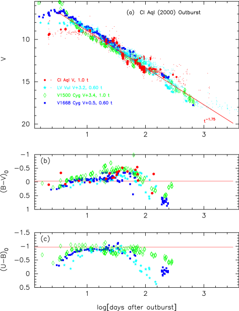
Figure 28: Light/color curves of the CI Aql (2000) outburst as well as LV Vul, V1500 Cyg, and V1668 Cyg. (a) The filled red circles and dots denote the $V$ and visual magnitudes of CI Aql, whereas the filled cyan stars, open green diamonds, and filled blue squares represent the $V$ magnitudes of LV Vul, V1500 Cyg, and V1668 Cyg, respectively. The data of LV Vul, V1668 Cyg, and V1500 Cyg are the same as those in Figures 4 and 1 of Hachisu & Kato (2016b), and Figure 6 of Hachisu & Kato (2014), respectively. These novae broadly follow the universal decline law of $F_{\nu}\propto t^{-1.75}$ (solid red line) (Hachisu & Kato, 2006). The (b) $(B-V)_{0}$ and (c) $(U-B)_{0}$ color curves. The colors of CI Aql are dereddened with $E(B-V)=1.0$.

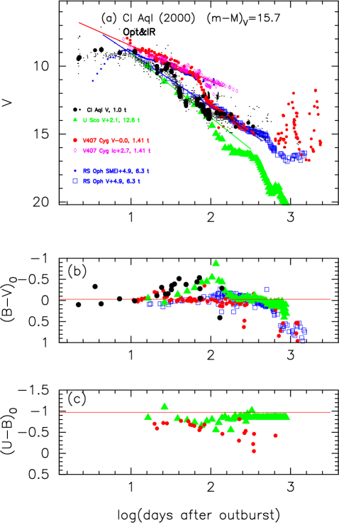
Figure 29: Same as Figure 24, but we plot the light/color curves of CI Aql (2000) as well as U Sco (2010), RS Oph (2006), and V407 Cyg. (a) The filled black circles and black dots denote the $V$ and visual magnitudes of CI Aql. The (b) $(B-V)_{0}$ and (c) $(U-B)_{0}$ color curves. The colors of CI Aql are dereddened with $E(B-V)=1.0$.

4.2 CI Aql (2000)

CI Aql is also a recurrent nova with three recorded outbursts in 1917, 1941, and 2000 (e.g., Schaefer, 2010). The maximum brightness and decline rates of the 2000 outburst were summarized as $m_{V,\rm max}=8.8$, $t_{2}=25$ days, and $t_{3}=32$ days by Strope et al. (2010). The WD mass was estimated by Hachisu et al. (2003) and Hachisu & Kato (2003) to be $M_{\rm WD}=1.2\pm 0.05~{}M_{\sun}$ from the model light curve fitting. The mass transfer rate and WD mass increasing rate were estimated to be $\dot{M}_{2}\sim-1\times 10^{-7}M_{\sun}$ yr^-1 and $\dot{M}_{\rm WD}=1.8\times 10^{-8}~{}M_{\sun}$ yr^-1, respectively, by Hachisu & Kato (2003). It takes $t_{\rm Ia}>(1.38-1.2)~{}M_{\sun}/1.8\times 10^{-8}~{}M_{\sun}$ yr${}^{-1}>1\times 10^{7}$ yr, during which time the companion will lose $\sim 1.0~{}M_{\sun}$ and the mass ratio will be reversed. Then the thermal timescale mass transfer cannot be maintained. We may conclude that CI Aql is not a progenitor of SNe Ia.

4.2.1 Universal decline law

Figure 28 shows the light/color curves of CI Aql on a logarithmic timescale. This figure also shows the light/color curves of the classical novae, LV Vul, V1500 Cyg, and V1668 Cyg. Although the $V$ light curve of CI Aql (2000) shows a wavy structure, these four novae broadly follow the universal decline law of $F_{\nu}\propto t^{-1.75}$ (solid red line). The horizontal shifts of $\log f_{\rm s}$ are essentially determined to overlap the $(B-V)_{0}$ color curves of these novae as shown in Figure 28. Once the horizontal shift is fixed, the vertical shift of $V$ light curve is uniquely determined. When the $V$ light curves obey the universal decline law and overlap each other, i.e., satisfy Equation (10), we can apply Equation (11) to Figure 28 and obtain the relation:

$$(m - M)_{V,\rm CI~{}Aql}$$ (64)

$$= (m-M+\Delta V)_{V,\rm LV~{}Vul}-2.5\log 0.60$$ (65)

$$= 11.9+3.2+0.55=15.65$$ (66)

$$= (m-M+\Delta V)_{V,\rm V1668~{}Cyg}-2.5\log 0.60$$ (67)

$$= 14.6+0.5+0.55=15.65$$ (68)

$$= (m-M+\Delta V)_{V,\rm V1500~{}Cyg}-2.5\log 1.0$$ (69)

$$= 12.3+3.4+0.0=15.7,$$ (70)

where we adopt $(m-M)_{V,\rm LV~{}Vul}=11.9$, $(m-M)_{V,\rm V1668~{}Cyg}=14.6$, and $(m-M)_{V,\rm V1500~{}Cyg}=12.3$ in Hachisu & Kato (2016b). We searched for the best overlap of CI Aql with V1668 Cyg and LV Vul but the vertical shifts of $\Delta V$ are not accurately determined because of its wavy structure of the $V$ light curve. Thus, we obtain $(m-M)_{V}=15.7\pm 0.5$ for CI Aql.

4.2.2 Reddening and distance

Figure 19(d) shows various distance-reddening relations toward CI Aql, whose galactic coordinates are $(l,b)=(31\fdg 6876,-0\fdg 8120)$. The relations of Marshall et al. (2006) are plotted in four directions close to the direction of CI Aql: $(l,b)=(31\fdg 50,-0\fdg 75)$ (open red squares), $(31\fdg 75,-0\fdg 75)$ (filled green squares), $(31\fdg 50,-1\fdg 00)$ (blue asterisks), and $(31\fdg 75,-1\fdg 00)$ (open magenta circles). The closest one is that shown with filled green squares. We added the relations of Green et al. (2015, 2018) (black and orange lines) and Özdörmez et al. (2016) (open cyan-blue diamonds). We adopt the reddening of $E(B-V)=1.0$ after Hachisu & Kato (2016b). The 3D distance-reddening relations of Marshall et al. and Green et al. (orange line), $(m-M)_{V}=15.7$ (solid blue line), and $E(B-V)=1.0$ (vertical solid red line) consistently cross each other at the distance of $d=3.3$ kpc and reddening of $E(B-V)=1.0$. Thus, we finally confirm that both the reddening of $E(B-V)=1.0$ and distance modulus in the $V$ band of $(m-M)_{V}=15.7$ are reasonable.

4.2.3 Color-magnitude diagram

Figure 27(b) shows the color-magnitude diagram of CI Aql. We identify the turning point (or cusp) to be $(B-V)_{0}=-0.52$ and $M_{V}=-3.84$, which is indicated by the large open red square. This turning point is on the two-headed black arrow given by Equation (5) of Hachisu & Kato (2016b). This property is common among U Sco and a number of classical novae, as discussed by Hachisu & Kato (2016b). The track of CI Aql almost overlaps with that of T Pyx. This again supports the set of $E(B-V)=1.0$ and $(m-M)_{V}=15.7$ for CI Aql.

4.2.4 Timescaling law and time-stretching method

Figure 29 compares CI Aql with RS Oph, V407 Cyg, and U Sco. If we adopt $(m-M)_{V}=15.7$ for CI Aql, the vertical shift of the $V$ light curve and horizontal shift of $\log f_{\rm s}$ are uniquely determined. We apply Equation (11) to Figure 29(a) to obtain the relation:

$$(m - M)_{V,\rm CI~{}Aql}=15.7$$ (71)

$$= (m-M+\Delta V)_{V,\rm RS~{}Oph}-2.5\log 6.3$$ (72)

$$= 12.8+4.9-2.0=15.7$$ (73)

$$= (m-M+\Delta V)_{V,\rm V407~{}Cyg}-2.5\log 1.41$$ (74)

$$= 16.1-0.0-0.38=15.72$$ (75)

$$= (m-M+\Delta V)_{V,\rm U~{}Sco}-2.5\log 12.6$$ (76)

$$= 16.3+2.1-2.75=15.65,$$ (77)

where we adopt $(m-M)_{V,\rm RS~{}Oph}=12.8$ in Section 3.1, $(m-M)_{V,\rm V407~{}Cyg}=16.1$ in Section 3.2, and $(m-M)_{V,\rm U~{}Sco}=16.3$ in Section 4.1. The $V$ light curve of CI Aql does not accurately overlap with the other three $V$ light curves, mainly because of the wavy shape. However, the global trend follows the other three $V$ light curves. Note that the $(B-V)_{0}$ color curve of CI Aql roughly overlaps with the trend of U Sco. In this sense, the time-stretching method of Equation (11) seems to be valid, even for the wavy $V$ light curve of CI Aql.

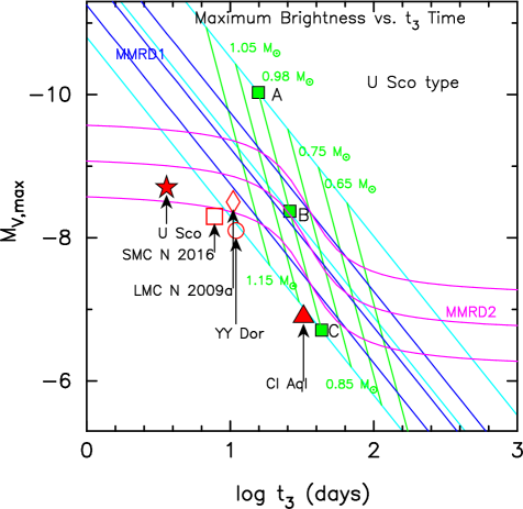
Figure 30: Same as Figure 16, but we plot U Sco (filled red star), CI Aql (filled red triangle), YY Dor (open red circles), LMC N 2009a (open red diamond), and SMC N 2016 (open red square). Here, we assume a distance of $20.4$ kpc for SMC N 2016. We also plot the MMRD lines (solid green lines) for the same WD mass but with different initial envelope masses (different ignition masses of the hydrogen-rich envelope). We plot 1.15, 1.05, 0.98, 0.85, 0.75, and $0.65~{}M_{\sun}$ WDs for the chemical composition of CO nova 3. The cyan line passing through point A (C) is a MMRD relation for a much larger (smaller) initial envelope mass than that of point B. The slope of these cyan lines is the same as that of MMRD1. See Appendix B for more detail.

4.3 MMRD relation of normal-decline type novae

We plot each MMRD point of the two recurrent novae, U Sco and CI Aql, in Figure 30. We added the same type of novae in LMC and SMC that are analyzed in Section 5. These normal-decline type novae are located slightly below or within the lower bound of MMRD1 and MMRD2. These locations can be understood in terms of small ignition masses, where the ignition mass is the hydrogen-rich envelope mass at the start of a nova outburst.

Hachisu & Kato (2010) theoretically examined the MMRD law for the galactic classical novae on the basis of the universal decline law. They concluded that the main trend of the MMRD relation is governed by the WD mass, i.e., the timescaling factor of $f_{\rm s}$ is the main parameter. The second parameter is the ignition mass, which determines the deviation from the main trend. To show the dependences, we plot the MMRD relations (solid green lines) in Figure 30 for the same WD mass but with different initial envelope masses. Here, we plot 1.15, 1.05, 0.98, 0.85, 0.75, and $0.65~{}M_{\sun}$ WDs for the chemical composition of CO nova 3, which are taken from Figure 51 of Appendix B.

There are three points denoted by A, B, and C on the $0.98~{}M_{\sun}$ WD model in Figure 30. The classical nova V1668 Cyg is located on point B. A nova on point A starts from a much larger envelope mass (smaller mass-accretion rate) than that of V1668 Cyg whereas a nova on point C has a much smaller envelope mass at ignition (larger mass-accretion rate) than that of V1668 Cyg even if they have the same WD mass as that of V1668 Cyg. The three cyan lines passing through points, A, B, and C, represent the model MMRD relations derived in Appendix B. These three cyan lines envelop the distribution of the classical novae studied by Downes & Duerbeck (2000) as shown in Figure 51 of Appendix B. The upper bound cyan line represents the case of larger envelope mass at ignition and the lower bound cyan line indicates that of smaller envelope mass at ignition for different WD masses.

In Figure 30, the normal-decline type novae are located almost on the lower bound of, or slightly below, the broad MMRD relation (cyan lines). These locations are theoretically understood in terms of small initial envelope masses, but the location of U Sco is slightly lower. This may be related to the shorter recurrence period of U Sco ($\sim 10$ yr) than the other ($\sim 20$ yr or more). The larger the mass-accretion rate is, the smaller the ignition mass is (e.g., Kato et al., 2014). Thus, the normal-decline type novae can be understood based on the universal decline law ($F_{\nu}\propto t^{-1.75}$). We may conclude that the normal-decline type novae have the same properties as those of classical novae that follow the universal decline law and do not belong to the faint class claimed by Kasliwal et al. (2011).

4.4 Summary of normal-decline (U Sco) type novae

We have analyzed the two recurrent novae, U Sco and CI Aql. The decay of optical and NIR light curves broadly follows the universal decline of $F_{\nu}\propto t^{-1.75}$ (Hachisu & Kato, 2006). If we properly stretch the timescales and shift up or down the $V$ magnitudes, we showed that these novae broadly obey the timescaling law of Equation (10) and the time-stretching method of Equation (11) is valid for these two novae. Although the $V$ light curve of CI Aql shows a wavy structure and does not exactly follow the universal decline law, we call these novae the normal decline (or U Sco) type novae.

We summarize the results of the two normal-decline (U Sco) type novae.

1. We have estimated the distance, reddening, and distance modulus of U Sco from various literature and methods after Hachisu & Kato (2016b). The results are summarized in Table 1.

2. We have also estimated the distance, reddening, and distance modulus of CI Aql from various literature and methods. The results are summarized in Table 1.

3. The $V$ light curve of U Sco decays as $F_{\nu}\propto t^{-1.75}$ in the early phase and then drops as $F_{\nu}\propto t^{-3.5}$.

4. The $V$ light curves of CI Aql shows a wavy structure but its global trend roughly follows the universal trend of $F_{\nu}\propto t^{-1.75}$.

5. We confirm that these two novae broadly overlap, i.e., satisfy Equation (10) and the time-stretching method, i.e., Equation (11).

6. These two novae are located at the lower bound of the law of Della Valle & Livio (MMRD2). CI Aql is located at the lower side of Kaler-Schmidt’s law (MMRD1) but U Sco is slightly fainter than this trend.

7. The WD mass of U Sco was estimated to be $M_{\rm WD}=1.37~{}M_{\sun}$ from the model light curve fitting (Hachisu et al., 2000a). This WD mass is so close to the explosion mass of SN Ia, $M_{\rm Ia}=1.38~{}M_{\sun}$ (Nomoto, 1982). The WD mass increases now (Hachisu et al., 2000a). This suggests that U Sco is a promising progenitor of SNe Ia.

8. The WD mass of CI Aql is estimated to be $M_{\rm WD}=1.2\pm 0.05~{}M_{\sun}$ (Hachisu & Kato, 2003) from the light curve fitting. The WD mass increases now (Hachisu & Kato, 2003) but it takes $t_{\rm Ia}>(1.38-1.2)~{}M_{\sun}/1.8\times 10^{-8}~{}M_{\sun}$ yr${}^{-1}>1\times 10^{7}$ yr, during which the companion will lose $\sim 1.0~{}M_{\sun}$ and the mass ratio will be reversed. The thermal timescale mass transfer cannot be maintained. Therefore, CI Aql is probably not a progenitor of SNe Ia.

5 Novae in Magellanic Clouds and M31

This is the first time that we apply our time-stretching method to extra-galactic novae, i.e., LMC, SMC, and M31. Their distances are generally well determined, and thus it is a good litmus test for our time-stretching method. We also observe if there are any characteristic differences between these novae and galactic novae, especially owing to the difference in the metallicity. We analyze YY Dor (2004), Nova LMC 2009a, Nova LMC 2012a, Nova LMC 2013 in LMC, and Nova SMC 2016 in SMC, and M31 N 2008-12a (2015) in M31. For LMC, we use the distance modulus of $\mu_{0}=18.5$ (Pietrzyński et al., 2013) and the reddening of $E(B-V)=0.12$ (Imara & Blitz, 2007) and neglect the difference in the reddening inside LMC unless otherwise specified.

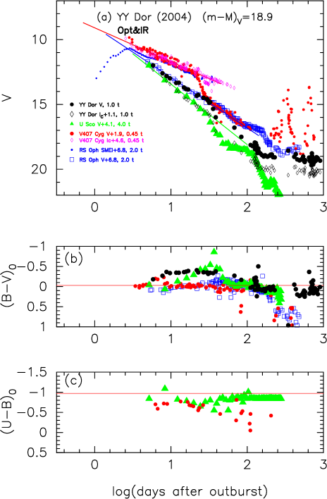
Figure 31: Same as Figure 24, but for the light/color curves of YY Dor (2004) as well as U Sco, V407 Cyg, and RS Oph. The data of YY Dor are taken from SMARTS. (a) The filled black circles denote the $V$ magnitudes of YY Dor, whereas the filled green triangles, filled red circles, and open blue squares denote the $V$ magnitudes of U Sco, V407 Cyg, and RS Oph, respectively. The $I_{C}$ magnitudes (open black diamonds) of YY Dor are added. The (b) $(B-V)_{0}$ and (c) $(U-B)_{0}$ color curves. The colors of YY Dor are dereddened with $E(B-V)=0.12$. See the text for detail.

5.1 YY Dor (2004)

YY Dor is a recurrent nova in LMC with two recorded outbursts in 1937 and 2004 (e.g., Bond et al., 2004; Shafter, 2013; Mason & Munari, 2014). The brightness reaches $m_{V,\rm max}=10.8$ (Liller et al., 2004) and the decline rates are estimated to be $t_{2}=4.0$ days and $t_{3}=10.9$ days (Walter et al., 2012). The distance modulus in the $V$ band is $(m-M)_{V}=\mu_{0}+A_{V}=18.5+3.1\times 0.12=18.9$, where $A_{V}=3.1\times E(B-V)$ is the absorption in the $V$ band.

Figure 31 shows the (a) $V$ and $I_{C}$ light curves and (b) $(B-V)_{0}$ color curve of YY Dor (2004). The data of YY Dor are taken from SMARTS (Walter et al., 2012). We explain our procedure of overlapping the nova light curves. In Figure 31(a), the $V$ light curve of YY Dor has a slope of $F_{\nu}\propto t^{-1.55}$ rather than $F_{\nu}\propto t^{-1.75}$. Therefore, we overlap it to the $V$ light curve of RS Oph rather than that of U Sco. We adopt $(m-M)_{V,\rm YY~{}Dor}=18.9$ and apply Equation (11) to the set of YY Dor and RS Oph. Then, we have

$$(m - M)_{V,\rm YY~{}Dor}=18.9$$ (78)

$$= (m-M+\Delta V)_{V,\rm RS~{}Oph}-2.5\log f_{\rm s}$$ (79)

$$= 12.8+\Delta V-2.5\log f_{\rm s},$$ (80)

where we adopt $(m-M)_{V,\rm RS~{}Oph}=12.8$ in Section 3.1. In this case, we have the relation:

$$\Delta V-2.5\log f_{\rm s}=6.1.$$ (81)

We change the value of $\Delta V$ in steps of 0.1 mag, obtain $\log f_{\rm s}$ from Equation (81), and plot the $V$ light curve of YY Dor for the set of $\Delta V$ (vertical shift) and $\log f_{\rm s}$ (horizontal shift). We search for the best-fit position of overlapping, as shown in Figure 31(a). In this case, we finally obtain $\Delta V=6.8$ and $\log f_{\rm s}=0.3$ ($f_{\rm s}=2.0$). After this procedure, the other two, V407 Cyg and U Sco, are fixed automatically because the overlapping positions of U Sco, V407 Cyg, and RS Oph are already known in Figure 24. Thus, we obtain the vertical and horizontal shifts of $\Delta V$ and $\log f_{\rm s}$ for these novae.

We also plot the $I_{C}$ light curve (open black diamonds) of YY Dor in Figure 31(a) in order to confirm that our horizontal fit is reasonable. The $I_{C}$ light curve has a slope of $F_{\nu}\propto t^{-1.75}$ and its break of the slope coincides with the break of U Sco $V$ light curve for the horizontal shift of $\log f_{\rm s}=0.3$. Thus, we conclude that YY Dor belongs to the U Sco type (normal decline), although its $V$ light curve has a slope of $F_{\nu}\propto t^{-1.55}$.

Now, we examine whether the time-stretching method is applicable to LMC novae. Using $(m-M)_{V}=18.9$ for YY Dor, we apply Equation (11) to all the novae in Figure 31(a) and obtain the relation:

$$(m - M)_{V,\rm YY~{}Dor}=18.9$$ (82)

$$= (m-M+\Delta V)_{V,\rm RS~{}Oph}-2.5\log 2.0$$ (83)

$$= 12.8+6.8-0.75=18.85$$ (84)

$$= (m-M+\Delta V)_{V,\rm V407~{}Cyg}-2.5\log 0.45$$ (85)

$$= 16.1+1.9+0.88=18.88$$ (86)

$$= (m-M+\Delta V)_{V,\rm U~{}Sco}-2.5\log 4.0$$ (87)

$$= 16.3+4.1-1.5=18.9,$$ (88)

where we adopt $(m-M)_{V,\rm RS~{}Oph}=12.8$ in Section 3.1, $(m-M)_{V,\rm V407~{}Cyg}=16.1$ in Section 3.2, and $(m-M)_{V,\rm U~{}Sco}=16.3$ in Section 4.1. These values are close to $(m-M)_{V,\rm YY~{}Dor}=18.9$. Thus, we confirm that the set of YY Dor, U Sco, V407 Cyg, and RS Oph consistently overlap with each other in the early phase, i.e., satisfy the timescaling law of Equation (10) and, at the same time, satisfy the time-stretching method of Equation (11).

Figure 32 shows the $I_{C}$ and $K_{s}$ light curves of YY Dor, U Sco, and LMC N 2009a. We also add the $I_{C}$ light curve of SMC N 2016 in Figure 32(a). This figure is essentially the same as Figure 25, but we plot the other light curves against YY Dor. These three novae have a slope of $F_{\nu}\propto t^{-1.75}$ (green lines) in the $I_{C}$ and $K_{s}$ light curves and overlap with the same scaling factors of $f_{\rm s}$ as that of the $V$ light curves. The distance modulus in the $I_{C}$ band is calculated to be $(m-M)_{I,\rm YY~{}Dor}=18.5+1.5\times 0.12=18.7$. We apply Equation (11) to all the novae and obtain

$$(m - M)_{I,\rm YY~{}Dor}=18.7$$ (89)

$$= (m-M+\Delta I_{C})_{I,\rm U~{}Sco}-2.5\log 4.0$$ (90)

$$= 15.9+4.3-1.5=18.7$$ (91)

$$= (m-M+\Delta I_{C})_{I,\rm LMC~{}N~{}2009a}-2.5\log 0.63$$ (92)

$$= 18.8-0.6+0.5=18.7$$ (93)

$$= (m-M+\Delta I_{C})_{I,\rm SMC~{}N~{}2016}-2.5\log 1.0$$ (94)

$$= 16.7+2.0-0.0=18.7,$$ (95)

where we adopt $(m-M)_{I,\rm U~{}Sco}=16.3-1.6\times 0.26=15.9$ from Section 4.1, $(m-M)_{I,\rm LMC~{}N~{}2009a}=18.5+1.5\times 0.2=18.8$ from Section 5.2, and $(m-M)_{I,\rm SMC~{}N~{}2016}=16.7$ from Section 5.5 in advance. Thus, we confirm that the set of YY Dor, U Sco, LMC N 2009a, and SMC N 2016 consistently overlap with each other in the early phase, i.e., satisfy the timescaling law of Equation (10) and, at the same time, satisfy the time-stretching method of Equation (11).

For the $K_{s}$ light curves, we similarly obtain

$$(m - M)_{K,\rm YY~{}Dor}=18.5+0.35\times 0.12=18.5$$ (96)

$$= (m-M+\Delta K_{s})_{K,\rm U~{}Sco}-2.5\log 4.0$$ (97)

$$= 15.6+4.4-1.5=18.5$$ (98)

$$= (m-M+\Delta K_{s})_{K,\rm LMC~{}N~{}2009a}-2.5\log 0.63$$ (99)

$$= 18.6-0.6+0.5=18.5,$$ (100)

where we adopt $(m-M)_{K,\rm U~{}Sco}=16.3-2.75\times 0.26=15.6$ from Section 4.1, $(m-M)_{K,\rm LMC~{}N~{}2009a}=18.5+0.35\times 0.2=18.6$ from Section 5.2. Thus, we confirm that the set of YY Dor, U Sco, and LMC N 2009a satisfy the timescaling law of Equation (10) and the time-stretching method of Equation (11). Thus, we conclude that YY Dor (and LMC N 2009a) belong to the normal decline (U Sco) type.

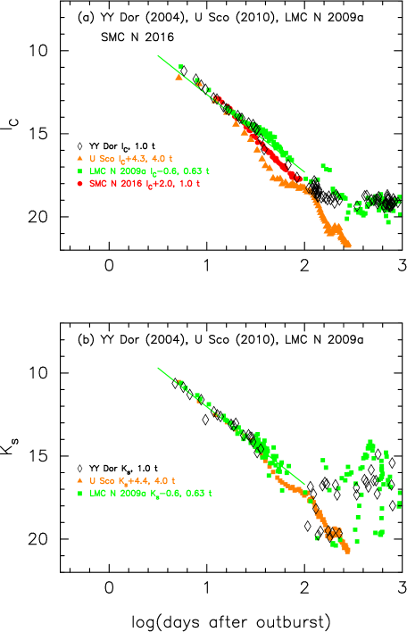
Figure 32: The (a) $I_{C}$ and (b) $K_{s}$ light curves of YY Dor (2004), U Sco (2010), and LMC N 2009a. We also add the $I_{C}$ light curve of SMC N 2016. Each light curve is horizontally stretched by $\log f_{\rm s}$ and vertically shifted by $\Delta I_{C}$ (or $\Delta K_{s}$). See the text for detail.

We plot the MMRD point of YY Dor in Figure 30. It lies in the lower side of the broad MMRD relations, close to the other members of the normal-decline type novae.

Figure 27(c) shows the color-magnitude diagram of YY Dor. We add a track (thin solid green lines) of V1668 Cyg shifted by $\Delta(B-V)=-0.3$ for comparison. The color-magnitude track of YY Dor almost overlaps with the blue-shifted V1668 Cyg track. We suppose that the reason for this blue-shift is the lower metallicity of LMC stars, [Fe/H]$=-0.55$ (see, e.g., Piatti & Geisler, 2013).

The WD mass of YY Dor is estimated to be $M_{\rm WD}=1.29~{}M_{\sun}$ from the linear relation between $M_{\rm WD}$ and $\log f_{\rm s}$ in Figure 17 (see Table 3 for the other WD masses). Although the exact recurrence period and orbital period of the binary are not known, we assume that the mass transfer rate and WD mass increasing rate are similar to those of CI Aql. Then, the mass transfer rate and WD mass increasing rate were estimated to be $\dot{M}_{2}\sim 1\times 10^{-7}M_{\sun}$ yr^-1 and $\dot{M}_{\rm WD}=1.8\times 10^{-8}~{}M_{\sun}$ yr^-1 by Hachisu & Kato (2003). It takes $t_{\rm Ia}>(1.38-1.29)~{}M_{\sun}/1.8\times 10^{-8}~{}M_{\sun}$ yr${}^{-1}>0.5\times 10^{7}$ yr, during which the companion will lose $\gtrsim 0.5~{}M_{\sun}$ and the mass ratio could be reversed. The thermal timescale mass transfer cannot be maintained. We may conclude that YY Dor is not a progenitor of SNe Ia.

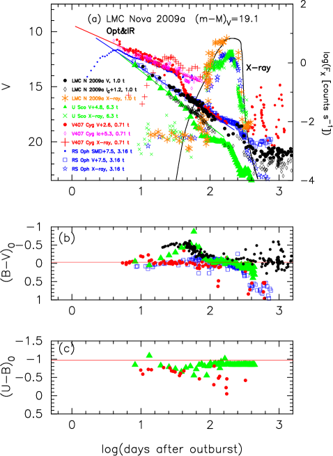
Figure 33: Same as Figure 24, but for LMC N 2009a. We included U Sco, V407 Cyg, and RS Oph for comparison. (a) The filled black circles denote the $V$ magnitudes and orange asterisks represent the X-ray flux of LMC N 2009a. The $I_{C}$ magnitudes (open black diamonds) of LMC N 2009a are added. The solid black line is the model supersoft X-ray flux of a $1.25~{}M_{\sun}$ WD with the chemical composition of Ne nova 3. The (b) $(B-V)_{0}$ and (c) $(U-B)_{0}$ color curves. The colors of LMC N 2009a are dereddened with $E(B-V)=0.2$.

5.2 Nova LMC 2009a

LMC Nova 2009a is a recurrent nova with recorded outbursts in 1971 and 2009. There was some confusion regarding the locations of the 1971 (1971b or 1971-08a) nova and 2009 (2009a or 2009-02a) nova. As a result, the recurrence was once suspected (e.g., Shafter, 2013; Mróz et al., 2016). Bode et al. (2016) remeasured the original plate of the 1971 outburst and confirmed that the 1971 nova position is the same as the 2009 nova position within 0$\farcs$1. The brightness reached $m_{\rm max}=10.6$ (unfiltered Kodak Technical Pan films by Liller, 2009). The decline rates are estimated to be $t_{2}=5.0$ days and $t_{3}=10.4$ days in the $V$ band (Bode et al., 2016). We assume that the $V$ maximum also reached $m_{V,\rm max}=10.6$. Figure 33 shows the (a) $V$ light curve and (b) $(B-V)_{0}$ color curve of LMC N 2009a. The data of LMC N 2009a are taken from SMARTS (Walter et al., 2012). Bode et al. (2016) reported pan-chromatic observations of LMC N 2009a, the emergence of the SSS phase at $63-70$ days, which was initially highly variable, and periodic modulations with $P=1.2$ days, which is most probably orbital in nature. They identified the progenitor system, i.e., the secondary is most likely a subgiant feeding a luminous accretion disk and suggested a WD mass of $1.1-1.3~{}M_{\sun}$ from the properties of the SSS phase. They also obtained the reddening $E(B-V)=A_{V}/3.1=0.6/3.1=0.2$ from the neutral hydrogen column density. Using this value, we calculate the intrinsic color of $(B-V)_{0}$ and plot them in Figure 33(b). The color evolution of LMC N 2009a is similar to that of U Sco. The distance modulus in the $V$ band is calculated to be $(m-M)_{V}=\mu_{0}+A_{V}=18.5+0.6=19.1$.

Using $(m-M)_{V}=19.1$ for LMC N 2009a, we confirm that the $V$ light curves of LMC N 2009a overlap to that of RS Oph and satisfy Equation (10) as shown in Figure 33. The slope of the $V$ light curve is close to that of RS Oph rather than U Sco while the slope of $I_{C}$ light curve (open black diamonds) is close to that of U Sco. Therefore, we conclude that LMC N 2009a belongs to the U Sco (normal decline) type. In the figure, we adopt the horizontal shift $\log f_{\rm s}=0.50$ of RS Oph against LMC N 2009a by overlapping the end of SSS phase of RS Oph (open blue stars) to that of LMC N 2009a (orange asterisks). Then, we apply Equation (11) to Figure 33 and obtain the relation:

$$(m - M)_{V,\rm LMCN~{}2009a}=19.1$$ (101)

$$= (m-M+\Delta V)_{V,\rm RS~{}Oph}-2.5\log 3.16$$ (102)

$$= 12.8+7.5-1.25=19.05$$ (103)

$$= (m-M+\Delta V)_{V,\rm V407~{}Cyg}-2.5\log 0.71$$ (104)

$$= 16.1+2.6+0.38=19.08$$ (105)

$$= (m-M+\Delta V)_{V,\rm U~{}Sco}-2.5\log 6.3$$ (106)

$$= 16.3+4.8-2.0=19.1,$$ (107)

where we adopt $(m-M)_{V,\rm RS~{}Oph}=12.8$ in Section 3.1, $(m-M)_{V,\rm V407~{}Cyg}=16.1$ in Section 3.2, and $(m-M)_{V,\rm U~{}Sco}=16.3$ in Section 4.1. From the close agreement of $(m-M)_{V}=19.1$, we confirm that the set of LMC N 2009a, U Sco, V407 Cyg, and RS Oph follow the timescaling law of Equation (10) and satisfy the time-stretching method of Equation (11).

With the same timescaling factors, we have already showed that the $I_{C}$ and $K_{s}$ light curves of LMC N 2009a, YY Dor, and U Sco overlap to each other and satisfy the time-stretching method of Equation (11) in Sections 4.1 and 5.1. These $I_{C}$ and $K_{s}$ light curves have a slope of $F_{\nu}\propto t^{-1.75}$, so we regard LMC N 2009a as a normal decline (U Sco) type. We plot the MMRD point in Figure 30. It is located in the lower bound of the broad MMRD relation.

Figure 27(d) shows the color-magnitude diagram of LMC N 2009a. The track of LMC N 2009a is in good agreement with the 0.2 mag blue-shifted V1500 Cyg and 0.15 mag blue-shifted U Sco tracks. The irradiated accretion disk contributes to the $B$, $V$, and $(B-V)$ below $M_{V}>-3$ and, as a result, the $(B-V)_{0}$ color is almost constant. The LMC N 2009a track overlaps to the 0.15 mag blue-shifted U Sco track. It should be noted that the turning point is located on the line of Equation (5) of Hachisu & Kato (2016b), i.e., the two-headed black arrow, in Figure 27(d). We again suppose that the bluer feature of the LMC N 2009a track is due to the lower metallicity of the LMC stars, as mentioned in Section 5.1.

The WD mass of LMC N 2009a is estimated to be $M_{\rm WD}=1.25~{}M_{\sun}$ from the linear relation between $M_{\rm WD}$ and $\log f_{\rm s}$ in Figure 17 (see Table 3 for the other WD masses). We plot the X-ray flux (solid black line) of a $1.25~{}M_{\sun}$ WD with the chemical composition of Ne nova 3 in Figure 33(a), which broadly reproduces the observation. If the orbital period is $1.2$ days, the companion is a subgiant, as in U Sco and CI Aql. The exact recurrence period is not known, but it is 38 yr or shorter. If we assume that the mass transfer rate and WD mass increasing rate are similar to those of CI Aql, it takes $t_{\rm Ia}>(1.38-1.25)~{}M_{\sun}/1.8\times 10^{-8}~{}M_{\sun}$ yr${}^{-1}>0.72\times 10^{7}$ yr, during which the companion will lose $\gtrsim 0.72~{}M_{\sun}$ and the mass ratio could be reversed. As a result, the thermal timescale mass transfer cannot be maintained. We may conclude that LMC N 2009a is not a progenitor of SNe Ia.

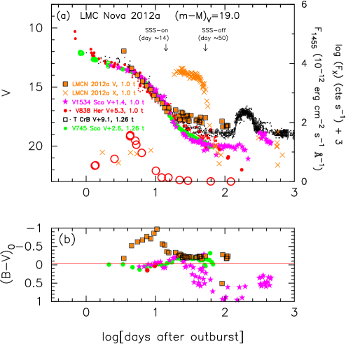
Figure 34: Same as Figure 13, but for the light/color curves of LMC N 2012a as well as V1534 Sco, V838 Her, T CrB, and V745 Sco. (a) The filled orange squares with black outlines denote the $V$ magnitudes of LMC N 2012a. The data are taken from SMARTS. The magenta crosses represent the Swift XRT X-ray flux ($0.3-10$ keV). The data are taken from the Swift web page (Evans et al., 2009). (b) The $(B-V)_{0}$ colors of LMC N 2012a are dereddened with $E(B-V)=0.15$.

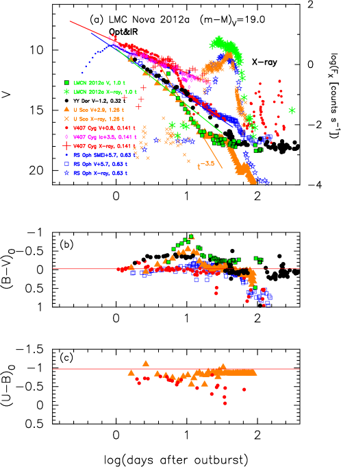
Figure 35: Same as Figure 33, but for the light/color curves of LMC N 2012a as well as YY Dor, U Sco, V407 Cyg, and RS Oph. (a) The filled green squares with black outlines denote the $V$ magnitudes of LMC N 2012a. The (b) $(B-V)_{0}$ and (c) $(U-B)_{0}$ color curves. The colors of LMC N 2012a are dereddened with $E(B-V)=0.15$.

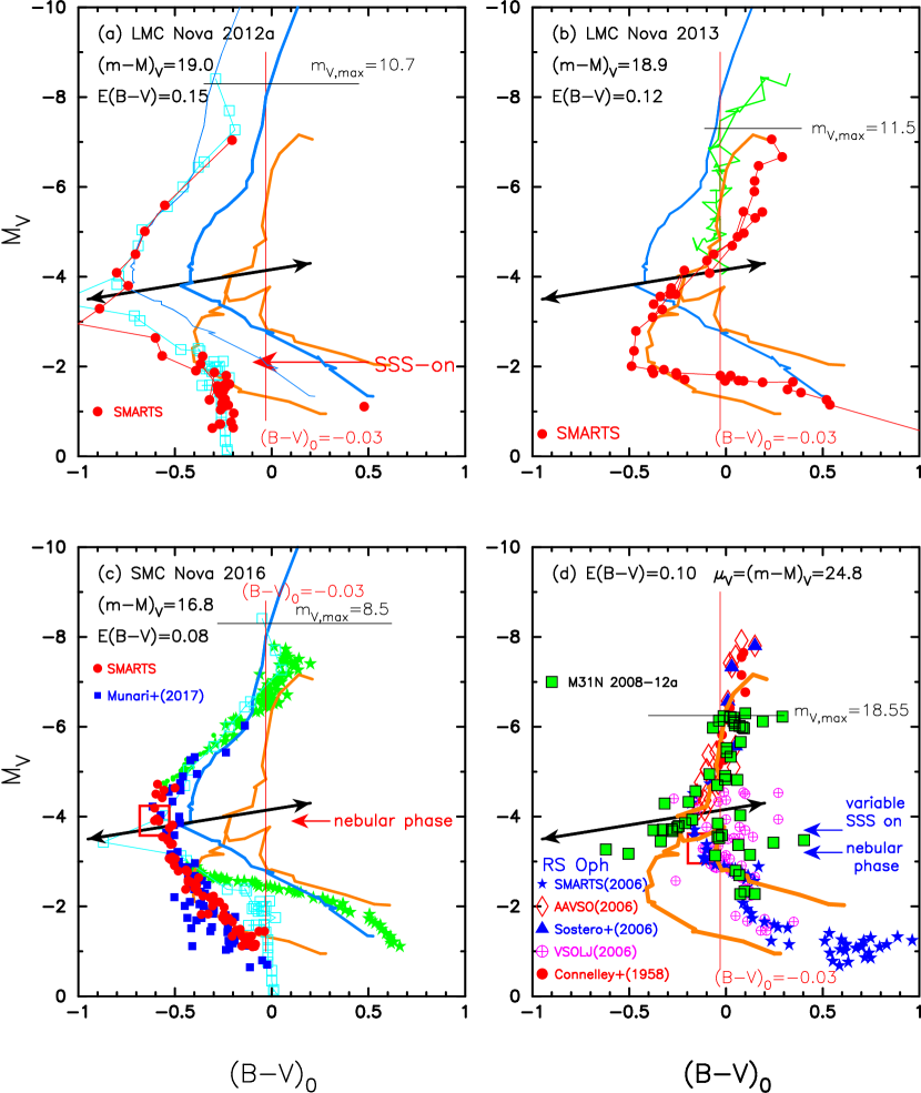
Figure 36: Same as Figure 6, but for (a) LMC N 2012a, (b) LMC N 2013, (c) SMC N 2016, and (d) M31N 2008-12a. The thick solid cyan-blue lines show the template track of V1500 Cyg, the thick solid orange lines show that of LV Vul, and the thick solid green lines show that of V1668 Cyg. In panel (a), we include a $\Delta(B-V)_{0}=-0.3$ mag blue-shifted track (thin solid cyan-blue line) of V1500 Cyg and $\Delta(B-V)_{0}=-0.25$ mag blue-shifted track (open cyan squares connected with thin solid cyan line) of U Sco (2010). In panel (c), we include the U Sco track (open cyan squares connected with thin solid cyan line) and T Pyx track (filled green stars). The large open red square denotes the start of the nebular phase, 23 days after optical maximum. In panel (d), we include the data of RS Oph, which are the same as those in Figure 16(a) of Hachisu & Kato (2016b). The filled green squares with black outlines denote M31N 2008-12a. Other symbols are all for RS Oph.

5.3 Nova LMC 2012a

LMC Nova 2012a reached maximum at $m_{\rm max}=10.7$ (digital SLR camera by Seach et al., 2012). The decline rates are estimated to be $t_{2}=1.1$ days and $t_{3}=2.1$ days in the $V$ band (Walter et al., 2012). We assumed that the $V$ maximum also reached $m_{V,\rm max}=10.7$. Figure 34 shows the (a) $V$ light curve and (b) $(B-V)_{0}$ color curve of LMC N 2012a. The data of LMC N 2012a are taken from SMARTS (Walter et al., 2012). Schwarz et al. (2015) reported the Swift and Chandra X-ray observations. The SSS phase started $13\pm 5$ days and ended approximately 50 days after the discovery. They obtained the orbital period of $19.24\pm 0.03$ hr (0.802 days) and the reddening of $E(B-V)=0.15$. We adopt this reddening and calculated the distance modulus in the $V$ band of $(m-M)_{V}=\mu_{0}+A_{V}=18.5+3.1\times 0.15=19.0$.

Using $(m-M)_{V}=19.0$ for LMC N 2012a, we confirm that the $V$ light curve of LMC N 2012a overlaps well with the $V$ light curves of V1534 Sco, V838 Her, T CrB, and V745 Sco. These five novae satisfy Equation (10). Then, we apply Equation (11) to Figure 34 and obtain the relation:

$$(m - M)_{V,\rm LMCN~{}2012a}=19.0$$ (108)

$$= (m-M+\Delta V)_{V,\rm V1534~{}Sco}-2.5\log 1.0$$ (109)

$$= 17.6+1.4+0.0=19.0$$ (110)

$$= (m-M+\Delta V)_{V,\rm V838~{}Her}-2.5\log 1.0$$ (111)

$$= 13.7+5.3+0.0=19.0$$ (112)

$$= (m-M+\Delta V)_{V,\rm T~{}CrB}-2.5\log 1.26$$ (113)

$$= 10.1+9.1-0.25=18.95$$ (114)

$$= (m-M+\Delta V)_{V,\rm V745~{}Sco}-2.5\log 1.26$$ (115)

$$= 16.6+2.6-0.25=18.95,$$ (116)

where we adopt $(m-M)_{V,\rm V1534~{}Sco}=17.6$ in Section 2.4, $(m-M)_{V,\rm V838~{}Her}=13.7$ in Section 2.3, $(m-M)_{V,\rm T~{}CrB}=10.1$ in Section 2.2, and $(m-M)_{V,\rm V745~{}Sco}=16.6$ in Section 2.1. We confirm that these novae satisfy Equation (11). We regard LMC N 2012a as a rapid-decline (V745 Sco) type nova. We plot the MMRD point of LMC N 2012a in Figure 16. The point is located closely to the other novae, and significantly below MMRD1 but slightly below MMRD2.

Figure 35 compares the light/color curves of LMC N 2012a with different types of novae, YY Dor, U Sco, V407 Cyg, and RS Oph. In this figure, there is no exhibit of $F_{\nu}\propto t^{-1.75}$, but one can observe $F_{\nu}\propto t^{-3.5}$ in the $V$ light curve of LMC N 2012a that overlaps with U Sco. This is because the initial envelope mass (ignition mass of hydrogen-rich envelope) is too small to reach the universal decline trend of $F_{\nu}\propto t^{-1.75}$, which is explained in more detail in Section 6.2. From Figure 35, we obtain the relation:

$$(m - M)_{V,\rm LMCN~{}2012a}=19.0$$ (117)

$$= (m-M+\Delta V)_{V,\rm YY~{}Dor}-2.5\log 0.32$$ (118)

$$= 18.9-1.2+1.25=18.95$$ (119)

$$= (m-M+\Delta V)_{V,\rm U~{}Sco}-2.5\log 1.26$$ (120)

$$= 16.3+2.9-0.25=18.95$$ (121)

$$= (m-M+\Delta V)_{V,\rm V407~{}Cyg}-2.5\log 0.141$$ (122)

$$= 16.1+0.8+1.13=19.03$$ (123)

$$= (m-M+\Delta V)_{V,\rm RS~{}Oph}-2.5\log 0.63$$ (124)

$$= 12.8+5.7+0.5=19.0,$$ (125)

where we adopt $(m-M)_{V,\rm YY~{}Dor}=18.9$ in Section 5.1, $(m-M)_{V,\rm U~{}Sco}=16.3$ in Section 4.1, $(m-M)_{V,\rm V407~{}Cyg}=16.1$ in Section 3.2, and $(m-M)_{V,\rm RS~{}Oph}=12.8$ in Section 3.1. Thus, we suggest that Equation (11) is satisfied by the set of LMC N 2012a, YY Dor, U Sco, V407 Cyg, and RS Oph even for the overlap in the part of $F_{\nu}\propto t^{-3.5}$. Comparing the timescaling factors between Figure 34 and Figure 35, we bridge the timescales between the two groups, V745 Sco and U Sco. Then, we obtain the common timescaling factors $f_{\rm s}$ among the three groups, as discussed in more detail in Section 6.1.

For the other bands, assuming the same timescaling factors, we have already compared the $B$ and $I_{C}$ light curves of LMC N 2012a with those of U Sco in Figure 26 of Section 4.1.2. Using the time-stretching method, we have obtained the distance and reddening of U Sco, because the distance and distance moduli of LMC N 2012a are well constrained.

Figure 36(a) shows the color-magnitude diagram of LMC N 2012a. The track of LMC N 2012a is in good agreement with the 0.3 mag blue-shifted V1500 Cyg (thin solid cyan-blue line) and 0.25 mag blue-shifted U Sco (open cyan squares connected with cyan line) tracks. The blue-shifted U Sco track overlaps well with that of LMC N 2012a, including the nearly constant $(B-V)_{0}$ phase below $M_{V}>-2$. The brightness and color of this SSS phase are dominated by the irradiated accretion disk. We regard that the lower metallicity environment in LMC is the cause of the bluer position of the color-magnitude track.

The WD mass of LMC N 2012a is estimated to be $M_{\rm WD}=1.37~{}M_{\sun}$ from the linear relation between $M_{\rm WD}$ and $\log f_{\rm s}$ in Figure 17 (see Table 3 for the other WD masses). It is unlikely that the WD was born as massive as $M_{\rm WD}\sim 1.37~{}M_{\sun}$ (Doherty et al., 2015). We suppose that the WD has grown in mass. This strongly suggests further increase in the WD masses in these systems. The orbital period is 0.802 days and the companion is a subgiant. Although the recurrence period is not known, we assume that the LMC N 2012a is a recurrent nova with a relatively short recurrence period, because the WD had grown in mass and the companion is a lobe-filling subgiant. If we further assume that the mass-increasing rate of WD is $\dot{M}_{\rm WD}\sim 1\times 10^{-7}~{}M_{\sun}$ yr^-1 just below the stability line of hydrogen-shell burning (Kato et al., 2017), the WD mass increases from $1.37~{}M_{\sun}$ to $M_{\rm Ia}=1.38~{}M_{\sun}$ and explodes as a SN Ia. It takes approximately $t_{\rm Ia}\sim 0.01~{}M_{\sun}/1\times 10^{-7}~{}M_{\sun}$ yr${}^{-1}=1\times 10^{5}$ yr, which is much shorter than the evolution timescale of the donor (subgiant star). Therefore, the WD will explode as a SN Ia if the core consists of carbon and oxygen. We suggest that LMC N 2012a is a promising progenitor of SNe Ia.

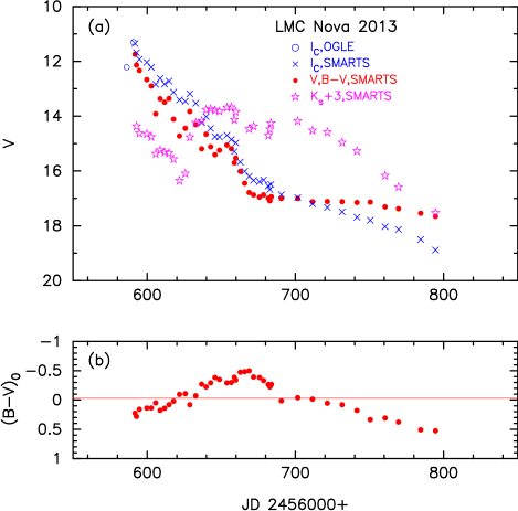
Figure 37: Same as Figure 20, but for LMC N 2013. (a) The $V$ (filled red circles), $I_{\rm C}$ (blue cross), and $K_{\rm s}$ (open magenta stars) data are taken from SMARTS. The $I_{\rm C}$ (open blue circles) data are from Mróz et al. (2015). (b) The $(B-V)_{0}$ data are taken from SMARTS and dereddened with $E(B-V)=0.12$.

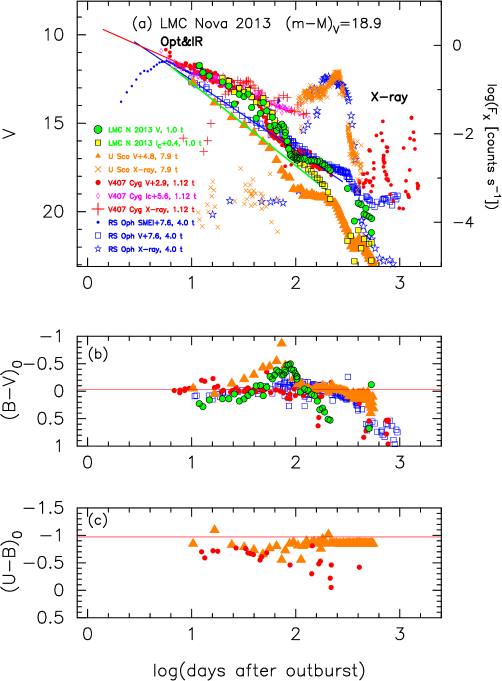
Figure 38: Same as Figure 33, but for the light/color curves of LMC N 2013 as well as U Sco, V407 Cyg, and RS Oph. (a) The filled green circles with black outlines denote the $V$ magnitudes of LMC N 2013. The $I_{C}$ magnitudes (filled yellow squares with black outlines) of LMC N 2013 are added. The (b) $(B-V)_{0}$ and (c) $(U-B)_{0}$ color curves. The $(B-V)_{0}$ colors of LMC N 2013 are dereddened with $E(B-V)=0.12$.

5.4 Nova LMC 2013

Figure 37 shows the (a) $V$, $I_{\rm C}$, and $K_{\rm s}$ light and (b) $(B-V)_{0}$ color curves of LMC N 2013 on a linear timescale. The $I_{\rm C}$ light curve decays almost linearly, whereas the $V$ light curve shows wavy structure with an amplitude of half a magnitude. The $K_{\rm s}$ magnitude (open magenta stars) sharply increases approximately 40 days after the outburst. A dust shell formed at this epoch, which was not so optically thick. The epoch of the $I_{\rm C}$ maximum is determined from the OGLE (open blue circles, Mróz et al., 2015) and SMARTS (blue crosses, Walter et al., 2012) data. The $I_{\rm C}$ magnitude reaches its maximum at $m_{I_{\rm C},{\rm max}}=11.3$ on JD 2456591.0. We regard that the $V$ brightness reaches $m_{V,\rm max}=11.5$ on the same day and estimate the decline rates as $t_{2}=21$ days and $t_{3}=47$ days from this figure.

We adopt $(m-M)_{V}=18.9$. Then, we determined the vertical shift $\Delta V$ and horizontal shift $\log f_{\rm s}$ for the set of LMC N 2013 and V407 Cyg by the same procedure as described in Section 5.1. The other timescaling factors $f_{\rm s}$ and vertical shifts $\Delta V$ are calculated from those in Figure 24. Thus, we plot the light/color curves of U Sco, V407 Cyg, and RS Oph against LMC N 2013 in Figure 38. We apply Equation (11) to Figure 38 and obtain the relation:

$$(m - M)_{V,\rm LMCN~{}2013}=18.9$$ (126)

$$= (m-M+\Delta V)_{V,\rm U~{}Sco}-2.5\log 7.9$$ (127)

$$= 16.3+4.8-2.25=18.85$$ (128)

$$= (m-M+\Delta V)_{V,\rm V407~{}Cyg}-2.5\log 1.12$$ (129)

$$= 16.1+2.9-0.13=18.87$$ (130)

$$= (m-M+\Delta V)_{V,\rm RS~{}Oph}-2.5\log 4.0$$ (131)

$$= 12.8+7.6-1.5=18.9,$$ (132)

where we adopt $(m-M)_{V,\rm U~{}Sco}=16.3$ in Section 4.1, $(m-M)_{V,\rm V407~{}Cyg}=16.1$ in Section 3.2, and $(m-M)_{V,\rm RS~{}Oph}=12.8$ in Section 3.1. Thus, LMC N 2013 and V407 Cyg satisfy Equations (10) and (11).

The $V$ light curve of LMC N 2013 shows a similar decline trend to that of V407 Cyg in the very early phase and then decays to the trend of RS Oph in the middle and later phase. Therefore, we regard LMC N 2013 as a CSM-shock (RS Oph) type nova. We plot the MMRD point of LMC N 2013 in Figure 22. The MMRD point of LMC N 2013 is located in the middle of the MMRD relations (both the MMRD1 and MMRD2 trends).

Figure 36(b) shows the color-magnitude diagram of LMC N 2013. The track of LMC N 2013 broadly follows the LV Vul track (thick solid orange lines) without blue-shifting. Comparing the LMC N 2013 track with that of LMC N 2012a (Figure 36(a), which overlaps with the 0.3 mag blue-shifted template), we suppose that LMC N 2013 has metallicity similar to those of galactic novae.

The WD mass of LMC N 2013 is estimated to be $M_{\rm WD}=1.23~{}M_{\sun}$ from the linear relation between $M_{\rm WD}$ and $\log f_{\rm s}$ in Figure 17 (see Table 3 for the other WD masses). Neither the orbital period nor the recurrence period is known. Even if we assume that the mass transfer rate and WD mass increasing rate are similar to CI Aql, it takes $t_{\rm Ia}>(1.38-1.23)~{}M_{\sun}/1.8\times 10^{-8}~{}M_{\sun}$ yr${}^{-1}>0.83\times 10^{7}$ yr, during which the companion will lose $\gtrsim 0.83~{}M_{\sun}$ and the mass ratio could be reversed before the WD mass reaches $M_{\rm Ia}=1.38~{}M_{\sun}$. We suppose that the thermal timescale mass transfer cannot be maintained until a SN Ia explosion. We may conclude that LMC N 2013 is not a progenitor of SNe Ia.

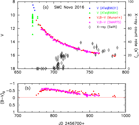
Figure 39: Same as Figure 37, but for SMC N 2016. (a) The $V$ (filled red circles) data are taken from Munari et al. (2017). The $V$ (filled magenta stars) data are from SMARTS. The filled blue circles (ATel No.9631) and filled green triangles (ATel No.9684) are the pre-discovery brightnesses of SMC N 2016 and taken from Lipunov et al. (2016) and Jablonski & Oliveira (2016), respectively. We also include the X-ray ($0.3-10$ keV) flux (open black diamonds) data taken from the Swift web site (Evans et al., 2009). (b) The $(B-V)_{0}$ are dereddened with $E(B-V)=0.08$.

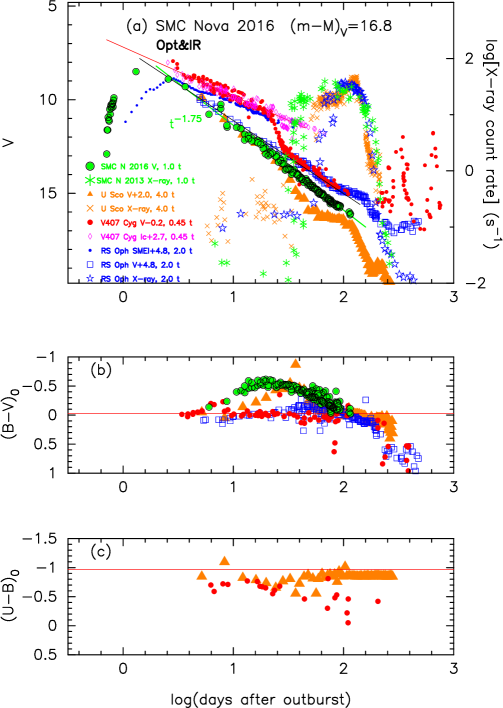
Figure 40: Same as Figure 38, but for the light/color curves of SMC N 2016. (a) The filled green circles with black outlines denote the $V$ magnitudes of SMC N 2016. The (b) $(B-V)_{0}$ and (c) $(U-B)_{0}$ color curves.

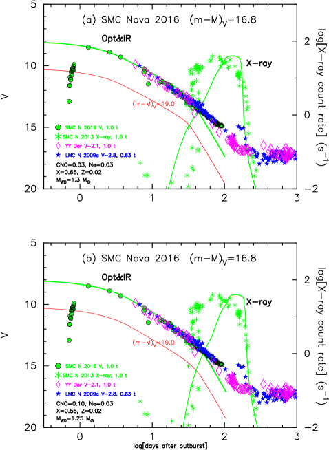
Figure 41: Same as Figure 40(a), but comparison with YY Dor and LMC N 2009a. The solid lines represent the model light curves of (a) a $1.3~{}M_{\sun}$ WD with the chemical composition of Ne nova 3, and (b) a $1.25~{}M_{\sun}$ WD of Ne nova 2. The green/red lines correspond to the model $V$ light curves for the distance modulus of $(m-M)_{V}=16.8$/19.0.

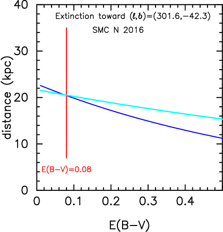
Figure 42: Various distance-reddening relation toward SMC N 2016 are plotted. The vertical solid red line denotes the reddening of $E(B-V)=0.08$. The blue and cyan lines indicate Equations (5) and (31) for $(m-M)_{V}=16.8$ and $(m-M)_{I}=16.7$, respectively.

5.5 Nova SMC 2016

SMC Nova 2016 (or 2016-10a) is located in the direction toward the outskirt of SMC, whose galactic coordinates are $(l,b)=(301\fdg 6362,-42\fdg 3037)$. Although Munari et al. (2017) and Aydi et al. (2018) assumed that SMC N 2016 is a member of SMC, we suppose that SMC N 2016 is a member of our galaxy, as discussed below.

Figure 39 shows the (a) $V$ light and (b) $(B-V)_{0}$ color curves of SMC N 2016. This nova was discovered by Shumkov et al. (2016) at mag 10.8 (unfiltered) on UT 2016 October 14.19. Lipunov et al. (2016) and Jablonski & Oliveira (2016) reported the pre-discovery brightnesses of SMC N 2016. The brightness reached $m_{\rm max}=8.5$ (unfiltered, Lipunov et al., 2016) and the decline rates were estimated to be $t_{2}=8.8$ days and $t_{3}=17.4$ days by Munari et al. (2017) or $t_{2}=4.0\pm 1.0$ days and $t_{3}=7.8\pm 2.0$ days by Aydi et al. (2018). Munari et al. (2017) also estimated the distance to be $d=44.8$ kpc and the reddening to be $E(B-V)=0.08$. Then, the distance modulus in the $V$ band is calculated to be $(m-M)_{V}=18.5$. The peak brightness is estimated from the MMRD relations to be $M_{V,\rm max}=-8.9$ or $-9.3$, depending on which MMRD relation is adopted. However, Aydi et al. (2018) obtained $M_{V,\rm max}=-10.5\pm 0.5$ and $(m-M)_{V}=19.0\pm 0.5$, assuming the distance of $d=61\pm 10$ kpc and absorption of $A_{V}=0.11\pm 0.06$.

Aydi et al. (2018) concluded that, if the nova is located in the SMC, it is the brightest nova ever discovered in the SMC and one of the brightest on record. Aydi et al. (2018) also showed that the total luminosity is as high as $10-20$ times the Eddington luminosity of a $1.2~{}M_{\sun}$ WD during the SSS phase (see their Figure 10). However, it is very unlikely that the total luminosity significantly exceeds the Eddington luminosity during the SSS phase. Evolution calculations clearly showed that the bolometric luminosity is close to the Eddington limit in the SSS phase (e.g., Sala & Hernanz, 2005; Denissenkov et al., 2013; Kato et al., 2017). This is because such large super-Eddington luminosity pushes the envelope against the gravity and expands the envelope. As a result, the photospheric temperature decreases below the supersoft X-ray emitting region. It seems more plausible that the distance to the nova is shorter by at least a factor of three, i.e., approximately $d\sim 20$ kpc, because the luminosity is just the Eddington luminosity during the SSS phase.

5.5.1 Time-stretching method

Figure 40 shows the same (a) $V$ light and (b) $(B-V)_{0}$ color curves of SMC N 2016 as in Figure 39 but on a logarithmic timescale. We included the $V$ light and $(B-V)_{0}$ color curves of U Sco, V407 Cyg, and RS Oph. We also included the supersoft X-ray fluxes of U Sco and RS Oph for comparison. Here, we determine the horizontal shifts $f_{\rm s}$ of each nova by overlapping the end of the SSS phase. The $V$ light and $(B-V)_{0}$ color curves of SMC N 2016 show a reasonable overlap with those of U Sco. Then, we determine the set of $\Delta V=2.0$ and $\log f_{\rm s}=0.6$ ($f_{\rm s}=4.0$) for SMC N 2016 and U Sco, as shown in Figure 40(a). We regard that Equation (10) is satisfied for SMC N 2016 and U Sco, because the $V$ light curves of these two novae nearly overlap with each other. Thus, we regard SMC N 2016 as a normal-decline (U Sco) type nova. We apply Equation (11) to all the novae in Figure 40 and obtain the relation:

$$(m - M)_{V,\rm SMC~{}N~{}2016}$$ (133)

$$= (m-M+\Delta V)_{V,\rm U~{}Sco}-2.5\log 4.0$$ (134)

$$= 16.3+2.0-1.5=16.8$$ (135)

$$= (m-M+\Delta V)_{V,\rm V407~{}Cyg}-2.5\log 0.45$$ (136)

$$= 16.1-0.2+0.88=16.78$$ (137)

$$= (m-M+\Delta V)_{V,\rm RS~{}Oph}-2.5\log 2.0$$ (138)

$$= 12.8+4.8-0.75=16.75,$$ (139)

where we adopt $(m-M)_{V,\rm U~{}Sco}=16.3$ in Section 4.1, $(m-M)_{V,\rm V407~{}Cyg}=16.1$ in Section 3.2, and $(m-M)_{V,\rm RS~{}Oph}=12.8$ in Section 3.1. Thus, we obtain $(m-M)_{V}=16.8$ for SMC N 2016.

Our value of $(m-M)_{V}=16.8$ yields the distance of $d=20.4$ kpc from Equation (5) together with $E(B-V)=0.08$ (Munari et al., 2017). Our distance is much shorter than the SMC distance of $d=61\pm 10$ kpc (Aydi et al., 2018). We contend that this nova belongs to our galaxy. It should be emphasized that this short distance is consistent with the above argument that the luminosity is just the Eddington luminosity during the SSS phase.

We check our distance of $d=20.4$ kpc to SMC N 2016 by comparing with the $V$ light curves of LMC novae, YY Dor and LMC N 2009a. Figure 41 shows that their $V$ light curves overlap to each other. We apply Equation (11) to all the novae and obtain

$$(m - M)_{V,\rm SMC~{}N~{}2016}=16.8$$ (140)

$$= (m-M+\Delta V)_{V,\rm YY~{}Dor}-2.5\log 1.0$$ (141)

$$= 18.9-2.1-0.0=16.8$$ (142)

$$= (m-M+\Delta V)_{V,\rm LMC~{}N~{}2009a}-2.5\log 0.63$$ (143)

$$= 19.1-2.8+0.5=16.8,$$ (144)

where we adopt $(m-M)_{V,\rm YY~{}Dor}=18.9$ from Section 5.1, $(m-M)_{V,\rm LMC~{}N~{}2009a}=19.1$ from Section 5.2. The distance moduli of YY Dor and LMC N 2009a are reliable because the two novae are members of LMC whose distance modulus is well constrained.

5.5.2 Model light curve fitting

Figure 41 also shows comparison with our model light curves. Figure 41(a) plots a $1.3~{}M_{\sun}$ WD model with the chemical composition of Ne nova 3 as a best-fit one among 1.2, 1.25, and $1.3~{}M_{\sun}$ WDs (Hachisu & Kato, 2016a). For Ne nova 2, we select the $1.25~{}M_{\sun}$ WD, which is shown in Figure 41(b), as a best-fit one among the three, 1.2, 1.25, and $1.3~{}M_{\sun}$ WDs (Hachisu & Kato, 2010). Note that the absolute magnitudes of these $V$ light curves are already known (Hachisu & Kato, 2010, 2016a). If we assume the distance modulus of $(m-M)_{V}=16.8$, we have a good fit (solid green line) with the observation. On the other hand, if we assume the SMC distance of $d=61$ kpc, that is, $(m-M)_{V}=19.0$ (Aydi et al., 2018), the model light curves (solid red lines) are much below the observation.

5.5.3 Distance-reddening relation

We further check our distance of $d=20.4$ kpc by the $I_{C}$ light curve. Figure 32(a) shows the $I_{C}$ light curves of SMC N 2016, YY Dor, U Sco, and LMC N 2009a. These four novae have a slope of $F_{\nu}\propto t^{-1.75}$ (green lines) in the $I_{C}$ light curves and overlap with the same scaling factors of $f_{\rm s}$ as those of the $V$ light curves. The distance modulus of SMC N 2016 in the $I_{C}$ band is calculated to be $(m-M)_{I,\rm SMC~{}N~{}2016}=16.8-1.6\times 0.08=16.7$. We apply Equation (11) to all the novae and obtain

$$(m - M)_{I,\rm SMC~{}N~{}2016}=16.7$$ (145)

$$= (m-M+\Delta I_{C})_{I,\rm YY~{}Dor}-2.5\log 1.0$$ (146)

$$= 18.7-2.0-0.0=16.7$$ (147)

$$= (m-M+\Delta I_{C})_{I,\rm U~{}Sco}-2.5\log 4.0$$ (148)

$$= 15.9+2.3-1.5=16.7$$ (149)

$$= (m-M+\Delta I_{C})_{I,\rm LMC~{}N~{}2009a}-2.5\log 0.63$$ (150)

$$= 18.8-2.6+0.5=16.7,$$ (151)

where we adopt $(m-M)_{I,\rm YY~{}Dor}=18.7$ from Section 5.1, $(m-M)_{I,\rm U~{}Sco}=15.9$ from Section 4.1, $(m-M)_{I,\rm LMC~{}N~{}2009a}=18.8$ from Section 5.2. Thus, we confirm that the set of SMC N 2016, YY Dor, U Sco, and LMC N 2009a consistently overlap with each other in the early phase, i.e., satisfy the timescaling law of Equation (10) and, at the same time, satisfy the time-stretching method of Equation (11).

Figure 42 shows various distance-reddening relations toward SMC N 2016. The vertical solid red line denotes the reddening of $E(B-V)=0.08$. The blue and cyan lines indicate the relations of Equations (5) and (31) for $(m-M)_{V}=16.8$ and $(m-M)_{I}=16.7$, respectively. These three lines cross consistently at the point of $d=20.4$ kpc and $E(B-V)=0.08$, supporting our estimate.

5.5.4 MMRD relation

We plot the MMRD point of SMC N 2016 in Figure 30. It is located closely to U Sco, LMC N 2009a, and YY Dor, and in the lower side of the broad MMRD relation. Thus, this nova is slightly fainter than the MMRD2 relation, not the brightest on record as argued by Aydi et al. (2018). We summarize the results in Tables 1, 2, and 3.

5.5.5 Color-magnitude diagram

Figure 36(c) shows the color-magnitude diagram of SMC N 2016. Here, we add two tracks of U Sco (open cyan squares connected by thin cyan lines) and T Pyx (filled green stars). The SMC N 2016 track broadly overlaps with those of U Sco and T Pyx. The start of the nebular phase (large open red square) is located on the two-headed arrow. This coincidence clearly shows that our adopted values of $E(B-V)=0.08$ and $(m-M)_{V}=16.8$ are reasonable and demonstrates that SMC N 2016 is a member of our galaxy. The distance of $d=20.4$ kpc is consistent with our overall understanding of the characteristic properties of novae.

5.5.6 Summary of SMC N 2016

The WD mass of SMC N 2016 is estimated to be $M_{\rm WD}=1.29~{}M_{\sun}$ from the linear relation between $M_{\rm WD}$ and $\log f_{\rm s}$ in Figure 17 (see Table 3 for the other WD masses). Aydi et al. (2018) discussed several constraints and summarized their results as $M_{\rm WD}>1.25~{}M_{\sun}$ from $t_{2}$ and $M_{\rm WD}\sim 1.25-1.3~{}M_{\sun}$ from the SSS duration, being consistent with our estimate both from the model light curve fitting in Figure 41 and linear relation of Figure 17. Neither the recurrence period nor the orbital period of the binary is known. If the evolutionary state is similar to CI Aql and YY Dor, we may conclude that SMC N 2016 is not a progenitor of SNe Ia.

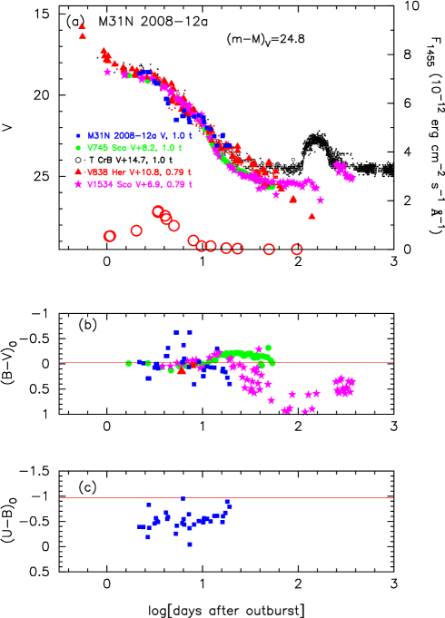
Figure 43: Same as Figure 34, but for the light/color curves of M31N 2008-12a. (a) The filled blue squares denote the $V$ magnitudes of M31N 2008-12a. The (b) $(B-V)_{0}$ and (c) $(U-B)_{0}$ color curves of M31N 2008-12a are dereddened with $E(B-V)=0.10$.

5.6 M31N 2008-12a (2015)

The 1-yr recurrence period nova M31N 2008-12a is an excellent example of recurrent novae because the distance and extinction are well determined (Darnley et al., 2015, 2016; Henze et al., 2015; Kato et al., 2015, 2016, 2017). The nova reached $m_{V,\rm max}=18.55$ and its decline rates are estimated to be $t_{2}=1.77$ days and $t_{3}=3.84$ days in the $V$ band (Darnley et al., 2016), being a very fast nova. Kato et al. (2015, 2016, 2017) concluded, on the basis of their multiwavelength light curve model, that the WD mass is close to $1.38~{}M_{\sun}$ and a promising candidate of SN Ia progenitors. The distance to M31 is $d\approx 780$ kpc and the extinction toward the nova is $E(B-V)\approx 0.1$ (e.g., Darnley et al., 2016). Then, the distance modulus is calculated to be $(m-M)_{V}=24.8$ from Equation (5).

With $(m-M)_{V}=24.8$ for M31N 2008-12a, the set of vertical shift $\Delta V$ and horizontal shift $\log f_{\rm s}$ are uniquely determined with the procedure described in Section 5.1. We overlap the $V$ light curve of M31N 2008-12a with those of V745 Sco, T CrB, V838 Her, and V1534 Sco, as shown in Figure 43. The $V$ light curve of M31N 2008-12a shows a quick decline a few days after the optical peak compared with the other rapid-decline (V745 Sco) type novae. Although the reason of this behavior is not identified yet, the decay trend recovers and again follows the other rapid-decline novae about 10 days after the outburst. Thus, we regard M31N 2008-12a as a rapid-decline type nova.

From Figure 43, we obtain $\Delta V=8.2\pm 0.3$ and $\log f_{\rm s}=0.0$ ($f_{\rm s}=1.0$) with respect to V745 Sco by overlapping the light curve in the early 1-3 days and late 10-20 days except the mid 4-9 days, because M31N 2008-12a shows a sharp decline during mid 4-9 days. We exclude T CrB and V838 Her from our fitting because these data show large scatter and are not appropriate. The $V$ light curve of M31N 2008-12a does not exactly but broadly overlap with V745 Sco and V1534 Sco. Thus, the vertical overlapping error could be as large as $\pm 0.3$ mag. We regard that these novae satisfy Equation (10). Then, we apply Equation (11) to M31N 2008-12a, V745 Sco, and V1534 Sco in Figure 43 and obtain the relation:

$$(m - M)_{V,\rm M31N~{}2008-12a}=24.8$$ (152)

$$= (m-M+\Delta V)_{V,\rm V745~{}Sco}-2.5\log 1.0$$ (153)

$$= 16.6+8.2+0.0=24.8$$ (154)

$$= (m-M+\Delta V)_{V,\rm V1534~{}Sco}-2.5\log 0.79$$ (155)

$$= 17.6+6.9+0.25=24.75,$$ (156)

where we adopt $(m-M)_{V,\rm V745~{}Sco}=16.6$ in Section 2.1 and $(m-M)_{V,\rm V1534~{}Sco}=17.6$ in Section 2.4. Thus, M31N 2008-12a, V745 Sco, and V1534 Sco satisfy Equations (10) and (11) within a vertical fitting error of $\pm 0.3$ mag. We regard M31N 2008-12a as a rapid-decline (V745 Sco) type nova. We plot the MMRD point of M31N 2008-12a in Figure 16. Its position is far below both the MMRD1 and MMRD2 relations. We may conclude that this nova belongs to the faint class, as claimed by Kasliwal et al. (2011).

Figure 36(d) shows the color-magnitude diagram of M31N 2008-12a (filled green squares with black outlines). The data for the 2014 outburst are taken from Darnley et al. (2015) and those for the 2015 outburst from Darnley et al. (2016). The peak brightness is approximately $M_{V}=18.55-24.8=-6.25$, being fainter than typical classical novae. The nova almost follows the track of RS Oph, which is a recurrent nova with a RG companion, although the $(B-V)_{0}$ data of M31N 2008-12a are rather scattered around $(B-V)_{0}=-0.03$. This resemblance may support our set of $E(B-V)=0.1$ and $(m-M)_{V}=24.8$ and a RG companion rather than a subgiant companion (see also discussion of Darnley et al., 2016).

Recently, Darnley et al. (2017) observed M31N 2008-12a in quiescence with HST and concluded that a quiescent disk mass accretion rate is the order of $10^{-6}~{}M_{\sun}$ yr^-1, based on their accretion disk model. This large accretion rate, however, clearly contradicts to the current theoretical understanding of nova outbursts because this accretion rate is far above the critical accretion rate for unstable nuclear burning (nova outbursts), several times $10^{-7}~{}M_{\sun}$ yr^-1 (see, e.g., Nomoto et al., 2007; Kato et al., 2014). Darnley et al. (2017) argued the possibility that a large part of accreted matter is blown in the accretion disk wind. We point out another possible explanation. Their disk model does not include the irradiation effect by the hot WD, which emits as much as $\sim 300~{}L_{\sun}$ (Kato et al., 2017). If the irradiation effect by the WD is included in their disk model, the accretion rate could be much smaller than their adopted value of $\sim 10^{-6}~{}M_{\sun}$ yr^-1 or more.

6 Discussion

6.1 Timescales over the three types

We have divided the 14 novae into three groups. In each group, we have determined the timescaling factor of $f_{\rm s}$ with respect to the template nova of the group. In this subsection, we determine the common timescales over the three groups. We adopt the timescale of V745 Sco as the unit of common timescale, which is the smallest $f_{\rm s}$ among the 14 novae.

The V745 Sco novae do not have the $F_{\nu}\propto t^{-1.75}$ slope, as shown in Figure 1. To determine the timescale difference between the V745 Sco and U Sco types, we use the slope of $F_{\nu}\propto t^{-3.5}$. In U Sco, this slope started approximately 10 days after the outburst (see Figures 1 and 23). We regard that the rapid-decline light curve of V745 Sco corresponds to the $F_{\nu}\propto t^{-3.5}$ decline of U Sco. This is because the ignition mass of the hydrogen-rich envelope of V745 Sco is too small to reach the slope of $F_{\nu}\propto t^{-1.75}$, and much smaller than that of U Sco.

Now, we determine the timescaling factor $f_{\rm s}$ of U Sco with respect to V745 Sco with the same procedure as in Sections 3.2.4 and 5.1. We overlap the V745 Sco and U Sco at the rapid decline trend of $F_{\nu}\propto t^{-3.5}$ and obtain the best overlap for the set of $\Delta V=0.3$ and $\log f_{\rm s}=0.0$ ($f_{\rm s}=1.0$), as shown in Figures 1 and 44. The timescaling factor of $f_{\rm s}$ is almost the same between these two novae, although their WD mass is slightly different. It is interesting that the start of the optically thin phase of V745 Sco and the start of the nebular phase (break) of U Sco roughly overlap. From Figures 1 and 44, we finally obtain

$$(m - M)_{V,\rm V745~{}Sco}=16.6$$ (157)

$$= (m-M+\Delta V)_{V,\rm RS~{}Oph}-2.5\log 0.50$$ (158)

$$= 12.8+3.0+0.75=16.55$$ (159)

$$= (m-M+\Delta V)_{V,\rm V407~{}Cyg}-2.5\log 0.112$$ (160)

$$= 16.1-1.9+2.38=16.58$$ (161)

$$= (m-M+\Delta V)_{V,\rm U~{}Sco}-2.5\log 1.0$$ (162)

$$= 16.3+0.3+0.0=16.6,$$ (163)

where we adopt $(m-M)_{V,\rm RS~{}Oph}=12.8$ in Section 3.1, $(m-M)_{V,\rm V407~{}Cyg}=16.1$ in Section 3.2, and $(m-M)_{V,\rm U~{}Sco}=16.3$ in Section 4.1, because we already know the difference in the timescale between RS Oph and U Sco. Figure 1 shows the relations between the template light curves for the four novae thus determined. The timescaling factor of each nova against that of V745 Sco is listed in Tables 1, 2, and 3.

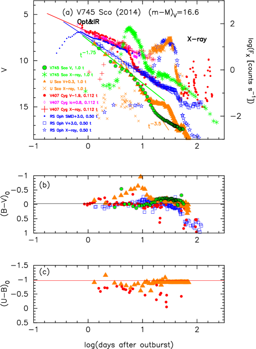
Figure 44: Same as Figure 35, but we plot the light/color curves of V745 Sco. (a) The filled green circles with black outlines denote the $V$ magnitudes of V745 Sco and the green asterisks represent the X-ray ($0.3-2.0$ keV) flux of V745 Sco, and the other symbols are the same as those in Figure 35. The (b) $(B-V)_{0}$ and (c) $(U-B)_{0}$ color curves. The $(B-V)_{0}$ colors of V745 Sco are dereddened with $E(B-V)=0.70$.

We have already tried to bridge the two timescales in the U Sco and LMC N 2012a light curve analysis (Sections 4.1 and 5.3). The above result is supported also by comparing the timescaling factors between Figures 34 and 35. The light curve of LMC N 2012a is similar to that of U Sco but has only $F_{\nu}\propto t^{-3.5}$ slope in the early decline phase. So we assign this nova to the V745 Sco group. Moreover, its absolute magnitude is well determined because of its LMC membership. Therefore, LMC N 2012a is a best example for bridging the two groups as clearly demonstrated in Section 5.3. To confirm again the relation among these three novae, we plot the absolute $V$ light curves and $(B-V)_{0}$ color curves of V745 Sco, U Sco, and LMC N 2012a in Figure 45. The ordinate is $M_{V}-2.5\log f_{\rm s}$ instead of $M_{V}$. After time-stretch of each nova light curve, the absolute $M_{V}-2.5\log f_{\rm s}$ magnitude should overlap to each other. In this particular case, V745 Sco and U Sco are time-stretched with $f_{\rm s}=1.26$ against LMC N 2012a. The three $V$ light curves clearly overlap to each other on the line of $F_{\nu}\propto t^{-3.5}$. The $V$ light curves of V745 Sco and U Sco further overlap to each other even in the very early phase of the outburst. The $V$ light curves of U Sco and LMC N 2012a show a similar plateau of $M_{V}-2.5\log f_{\rm s}\sim-2$ mag, which is caused by a disk irradiation by the central WD (e.g., Hachisu et al., 2000a). Thus, we confirm that our common timescale between the V745 Sco and U Sco types supports Equation (11) and vice versa.

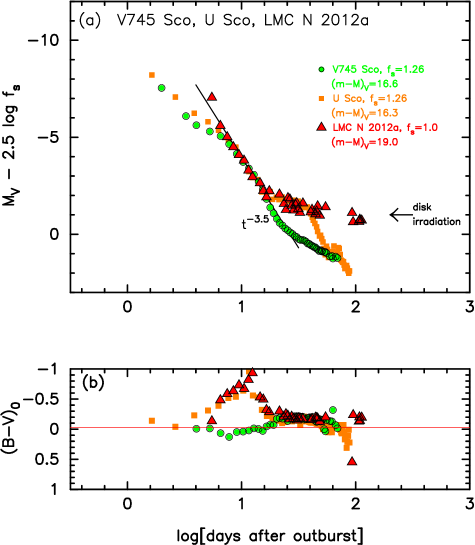
Figure 45: (a) The absolute $V$ light curves of V745 Sco, U Sco, and LMC N 2012a on a logarithmic timescale. The ordinate is $M_{V}-2.5\log f_{\rm s}$ instead of $M_{V}$. (b) The $(B-V)_{0}$ color curves of V745 Sco, U Sco, and LMC N 2012a.

6.2 Large deviation from MMRD relations

We have already examined the MMRD relation for many galactic classical novae based on our model light curves (Hachisu & Kato, 2010, 2015, 2016a). The main conclusions are that (1) the main trend is determined by the timescaling factor $f_{\rm s}$ (WD mass), (2) the scatter from the main trend is due to the difference in the ignition mass (mass accretion rate on to the WD), and (3) the saturation of the peak brightness for the longer ($t_{2}$ or) $t_{3}$ time regime (less massive WDs) is caused by the contribution from the photospheric radiation (see Hachisu & Kato, 2015, for more detail). In this subsection, we add new reasons for the scatter of MMRD points from the main trend, especially for recurrent and very fast novae.

We pointed out that there are three types of nova light curves, the normal-decline (U Sco), rapid-decline (V745 Sco), and CSM-shock (RS Oph) types. We discuss the three types in this order.

The light curves of the normal-decline (U Sco) novae closely follow the trend of the universal decline law, $F_{\nu}\propto t^{-1.75}$, as shown in Figure 1. Their MMRD points are located in the lower region of the MMRD relations, as shown in Figure 30. These deviations come from reason (2) mentioned above. This is because the ignition masses are relatively small in these novae, i.e., smaller initial envelope mass at hydrogen burning (point C rather than point B in Figures 30, 48, 49, and 51). Therefore, the peak brightness $M_{V,\rm max}$ is relatively faint, even for the smaller $t_{2}$ and $t_{3}$ times. This trend is the same as that in classical novae. We explain this effect in more detail in Appendix B.

The light curves of the rapid-decline (V745 Sco) type novae are characterized by a very short period before the start of SSS phase. Soon after the optical peak, the $V$ brightness quickly decays as $F_{\nu}\propto t^{-3.5}$, as shown in Figure 1. The start of quick decay from $F_{\nu}\propto t^{-1.75}$ to $F_{\nu}\propto t^{-3.5}$ roughly corresponds to the break of the U Sco $V$ light curve. (See also Figure 49 in Appendix A for the break). This means that the ignition mass of the hydrogen-rich envelope is too small to reach the normal-decline segment of $F_{\nu}\propto t^{-1.75}$. The $t_{2}$ and $t_{3}$ times are much shorter because $F_{\nu}\propto t^{-3.5}$ rather than $F_{\nu}\propto t^{-1.75}$. The peak brightness is fainter because of the smaller ignition mass and smaller wind mass-loss rate. Thus, this type of novae are located significantly below the MMRD relations, as shown in Figure 16. In short, this occurs when the ignition mass is much smaller than the case of the normal-decline types. We may conclude that the rapid-decline type novae do not exhibit $F_{\nu}\propto t^{-1.75}$ (the universal trend of galactic classical novae) in their early phase $V$ light curves, but start with $F_{\nu}\propto t^{-3.5}$ and the two novae, V1534 Sco and M31N 2008-12a, belong to the faint class claimed by Kasliwal et al. (2011).

The final case we discuss is the contamination of shock-heating. The light curves of the CSM-shock (RS Oph) type novae are contaminated by the flux from shock-heating, as shown in Figures 1, 18, 21, and 38. These show slow decline rates close to $F_{\nu}\propto t^{-1.0}$ during the strong shock-interaction with the CSM. Therefore, their $t_{2}$ and $t_{3}$ times are longer than those with no shock contamination, even for the same $M_{V,\rm max}$. These novae host a massive WD and the ignition mass is large enough to start from the decline of $F_{\nu}\propto t^{-1.75}$. Therefore, the naked MMRD points without shock contamination should be located in the lower side of the broad MMRD relations, like those of the normal-decline (U Sco) types. With the help of shock-heating, novae of this type happen to follow the MMRD relations as shown in Figure 22.

6.3 Progenitors of Type Ia supernovae

A typical evolution path of the progenitors in the SD scenario (e.g., Hachisu et al., 1999a, b) is as follows: When the companion evolves to expand and fills its Roche lobe, mass transfer begins from the companion to the WD. The mass transfer rate quickly increases and exceeds the critical rate for optically thick wind (see $\dot{M}_{\rm cr}$ in Figure 3 of Kato et al., 2014). The WD evolves from the optically thick wind phase, through the SSS phase (steady H-burning phase) and to the recurrent nova phase (H-shell flash phase), and finally explodes as a SN Ia (e.g., Hachisu et al., 2008a, 2012). The WD mass substantially increases during the wind and SSS phases before the WD enters a recurrent nova phase. In other words, a recurrent nova in the course toward a SN Ia has a WD that has already grown up to very close to the Chandrasekhar mass. A recurrent nova with a WD mass, say $1.2~{}M_{\sun}$, will not reach the Chandrasekhar mass in the ensuing binary evolution (e.g., Hachisu et al., 2008a, 2012).

Therefore, a SN Ia progenitor in a recurrent nova phase should host a WD close enough to $M_{\rm Ia}=1.38~{}M_{\sun}$ (Nomoto, 1982) before the SN Ia explosion, as mentioned in Section 1. The binary orbital period is highly likely in the ranges between $\sim$0.3 and $\sim$5 days for WD+MS binary systems, or between $\sim$100 and $\sim$1000 days for WD+RG binary systems (see, e.g., Figure 1 of Hachisu et al., 2008a). These orbital periods support high mass accretion rates onto the WDs and sufficient mass retention efficiency of the accreted matter. The typical mass-increasing rates of WDs are $\dot{M}_{\rm WD}\sim 1\times 10^{-7}~{}M_{\sun}$ yr^-1 just below the stability line of hydrogen-shell burning (see, e.g., Kato et al., 2017). If the WD mass increases from $1.35~{}M_{\sun}$ to $M_{\rm Ia}=1.38~{}M_{\sun}$ in the recurrent nova phase and explodes as a SN Ia, it takes approximately $t_{\rm Ia}\sim 0.03~{}M_{\sun}/1\times 10^{-7}~{}M_{\sun}$ yr${}^{-1}=3\times 10^{5}$ yr, which is shorter than the evolution timescale of the donor (RG star or MS star). It is unlikely that these WDs were born as massive as they are ($M_{\rm WD}\geq 1.35~{}M_{\sun}$). Therefore, these WDs have grown in mass since their births. This strongly suggests further increase in the WD masses in these systems.

Figure 17 shows the WD mass against the timescaling factor of $\log f_{\rm s}$, where the timescaling factor is measured based on that of V745 Sco ($f_{\rm s}=1.0$ for V745 Sco). Various WD masses are estimated from the trend of this $f_{\rm s}$ vs. $M_{\rm WD}$ relation (solid red lines). We also plot the WD masses determined by the other methods, as listed in Table 3. Among these 14 novae, we select eight novae that almost satisfy the conditions of SN Ia progenitor mentioned above, i.e., T CrB ($1.38~{}M_{\sun}$, RG, $P_{\rm orb}=227.6$ days), V838 Her ($1.37~{}M_{\sun}$, MS, $P_{\rm orb}=0.2976$ days), RS Oph ($1.35~{}M_{\sun}$, RG, $P_{\rm orb}=453.6$ days), U Sco ($1.37~{}M_{\sun}$, subgiant, $P_{\rm orb}=1.23$ days), V745 Sco ($1.385~{}M_{\sun}$, RG, $P_{\rm orb}=$unknown), V1534 Sco ($1.37~{}M_{\sun}$, RG, $P_{\rm orb}=$unknown), LMC N 2012a ($1.37~{}M_{\sun}$, subgiant, $P_{\rm orb}=0.802$ days), and M31N 2008-12a ($1.38~{}M_{\sun}$, RG?, $P_{\rm orb}=$unknown).

7 Conclusions

Our results are summarized as follows:

1. We analyzed 14 fast novae including eight recurrent novae, and divided them into three types of light curve shapes: the rapid-decline (V745 Sco), CSM-shock (RS Oph), and normal-decline (U Sco) types. The rapid-decline type includes V745 Sco, T CrB, V838 Her, V1534 Sco, LMC N 2012a, and M31N 2008-12a; the CSM-shock type includes RS Oph, V407 Cyg, and LMC N 2013; and the normal-decline type includes U Sco, CI Aql, YY Dor, LMC N 2009a, and SMC N 2016. We obtained the distances, distance moduli in the $V$ band, and reddenings of each nova from various methods. The results are summarized in Table 1.

2. The normal-decline type novae follow the universal decline trend of $F_{\nu}\propto t^{-1.75}$ in a substantial part of their early $V$ light curves. The CSM-shock type novae have a substantial part of $F_{\nu}\propto t^{-1.0}$ during shock-heating between ejecta and CSM. After the shock breakout, the slope changes to $F_{\nu}\propto t^{-1.55}$. The rapid-decline type novae have no or a very short duration of the universal trend of $F_{\nu}\propto t^{-1.75}$, but rather follow a steep trend of $F_{\nu}\propto t^{-3.5}$. This is because their initial envelope masses are too small to reach the normal-decline segment of $F_{\nu}\propto t^{-1.75}$, but they only start from a later phase in which the slope has already changed from $F_{\nu}\propto t^{-1.75}$ to $F_{\nu}\propto t^{-3.5}$.

3. Comparing the five nova light curves of V407 Cyg, RS Oph, V745 Sco, T CrB, and V1534 Sco that have a RG companion, we found that V407 Cyg is most heavily contaminated by shock-heating ($F_{\nu}\propto t^{-1.0}$), RS Oph is slightly weaker ($F_{\nu}\propto t^{-1.55}$ but $L_{\rm SMEI}\propto t^{-1.0}$) than V407 Cyg, V745 Sco and T CrB are much weaker ($F_{\nu}\propto t^{-3.5}$), and V1534 Sco is almost uncontaminated ($F_{\nu}\propto t^{-3.5}$).

4. In all three types of novae, the $V$ light curves follow a timescaling law (if we properly stretch or squeeze in the time direction and shift up or down each $V$ light curve), i.e., they almost overlap each other in the same group. We regard that they broadly obey Equation (10). Based on the obtained distance moduli, we confirm that these novae satisfy the time-stretching method, i.e., Equation (11) when they obey Equation (10).

5. We apply our methods, i.e., timescaling law and time-stretching method, to LMC, SMC, and M31 novae. This is our first attempt to apply the method to extra-galactic novae. We identified YY Dor, LMC N 2009a, and SMC N 2016 as the normal-decline type, LMC N 2013 as the CSM shock type, and LMC N 2012a and M31N 2008-12a as the rapid-decline type. We confirm that these novae also satisfy the time-stretching method when they overlap with each other, i.e., Equation (10) and Equation (11). These results support that the time-stretching method is applicable, even to M31 and LMC novae.

6. We find that SMC N 2016 is not a member of SMC, but rather a member of our galaxy, because its distance is obtained to be $d=20\pm 2$ kpc.

7. The rapid-decline type novae do not obey the MMRD relations, i.e., their MMRD points are much fainter. This is because their initial envelope masses, i.e., ignition masses, are too small to reach the universal decline of $F_{\nu}\propto t^{-1.75}$. The normal-decline type novae are located in the lower region of the law of Della Valle & Livio (MMRD2), but far below Kaler-Schmidt’s law (MMRD1). The CSM-shock type novae happen to be located near the main trend of the MMRD relations, because the light curves are contaminated with shock-heating and slowly decay as $F_{\nu}\propto t^{-1.0}$, resulting in longer $t_{2}$ and $t_{3}$ times that compensate the relatively faint $M_{V,\rm max}$. Thus, in general, the empirical MMRD relations should not be used to estimate the distance moduli of very fast and recurrent novae.

8. The WD mass of V745 Sco is estimated to be $M_{\rm WD}=1.385~{}M_{\sun}$ from our model light curve fitting with the supersoft X-ray light curve. This WD mass is more massive than $M_{\rm WD}=1.38~{}M_{\sun}$ of the 1-yr recurrence period nova, M31N 2008-12a. This is consistent with the earlier appearance of the SSS phase of V745 Sco ($t_{\rm SSS-on}\sim 4$ days) than that of M31N 2008-12a ($t_{\rm SSS-on}\sim 6$ days).

9. The WD mass of V838 Her is estimated to be $M_{\rm WD}=1.37~{}M_{\sun}$ from our model light curve fitting with the UV 1455 Å light curve. This is consistent with the timescaling factor $\log f_{\rm s}=0.1$ ($f_{\rm s}=1.26$) of V838 Her, which is slightly larger than $\log f_{\rm s}=0$ ($f_{\rm s}=1.0$) of V745 Sco ($M_{\rm WD}=1.385~{}M_{\sun}$) in the same V745 Sco group.

10. Among the analyzed 14 novae, we select eight novae that almost satisfy the conditions of SN Ia progenitors, i.e., T CrB ($M_{\rm WD}=1.38~{}M_{\sun}$), V838 Her ($1.37~{}M_{\sun}$), RS Oph ($1.35~{}M_{\sun}$), U Sco ($1.37~{}M_{\sun}$), V745 Sco ($1.385~{}M_{\sun}$), V1534 Sco ($1.37~{}M_{\sun}$), LMC N 2012a ($1.37~{}M_{\sun}$), and M31N 2008-12a ($1.38~{}M_{\sun}$).

Appendix A Model Light Curves of Novae

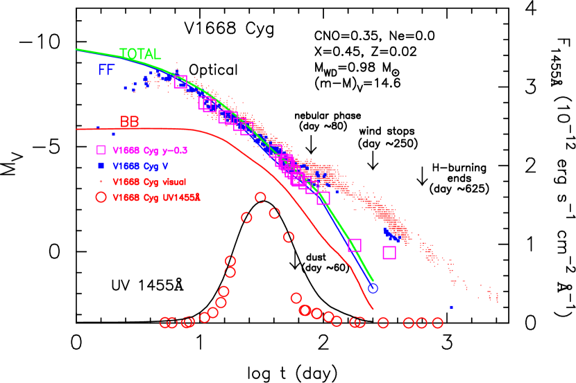
Figure 46: Visual (red dots), $V$ (filled blue circles), and $y$ (open magenta squares) light curves and UV 1455 Å light curve (large open red circles) of V1668 Cyg. Assuming that $(m-M)_{V}=14.6$, we plot three model light curves of a $0.98~{}M_{\sun}$ WD. The green, blue, and red solid lines show the total (labeled “TOTAL”), free-free (labeled “FF”), and blackbody (labeled “BB”) $V$ fluxes. The solid black line denotes the UV 1455 Å flux. An optically thin dust shell formed $\sim 60$ days after the outburst (e.g., Gehrz et al., 1980). Optically thick winds and hydrogen-shell burning end approximately 250 and 625 days after the outburst, respectively, for the $0.98~{}M_{\sun}$ WD model.

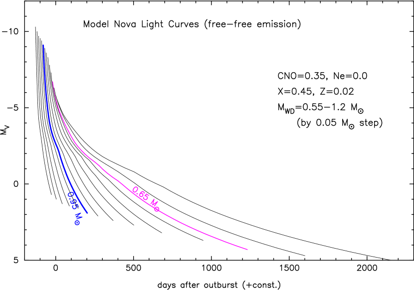
Figure 47: Absolute $V$ magnitudes of free-free emission model light curves for the chemical composition of CO nova 3 and WD masses of $0.55-1.2~{}M_{\sun}$ in $0.05~{}M_{\sun}$ steps, the numerical data of which are taken from Table 3 of Hachisu & Kato (2016a). The mass of hydrogen-rich envelope on the WD gradually decreases along each light curve because the envelope mass is lost in the wind and consumed by nuclear burning. The right edges of free-free emission model light curves correspond to the epoch when the optically thick winds stop. Two light curves are specified by the thick solid magenta line ($0.65~{}M_{\sun}$) and thick solid blue line ($0.95~{}M_{\sun}$). A less massive WD declines more slowly, and thus the nova speed class depends mainly on the WD mass.

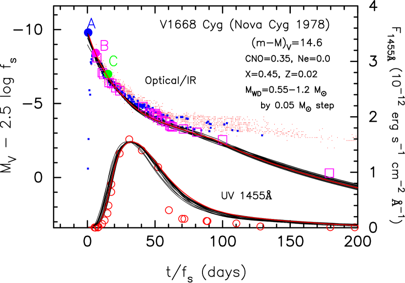
Figure 48: Same model light curves as in Figure 47, but in the $(t/f_{\rm s})$-$(M_{V}-2.5\log f_{\rm s})$ coordinates. We add the UV 1455 Å model light curves. The optical and UV 1455 Å data of V1668 Cyg are the same as those in Figure 3 of Hachisu & Kato (2016a). The UV 1455 Å model fluxes are normalized to the peak value of the UV observation. We measure the timescaling factor $f_{\rm s}$ of each model with respect to the V1668 Cyg light curves. The values of $\log f_{\rm s}$ are tabulated in Table 3 of Hachisu & Kato (2016a). All the free-free emission model light curves overlap with each other in the $M_{V}-2.5\log f_{\rm s}$ ordinate and the $t/f_{\rm s}$ abscissa. We add a $0.98~{}M_{\sun}$ WD model (solid red lines), which simultaneously reproduce the $V$ (filled blue squares), $y$ (large open magenta squares), and UV 1455 Å (large open red circles) light curves of V1668 Cyg. Three different initial envelope masses of $M_{\rm env,0}=2.0\times 10^{-5}M_{\sun}$, $1.4\times 10^{-5}M_{\sun}$, and $0.93\times 10^{-5}M_{\sun}$ correspond to the three peak brightnesses, i.e., points A, B, and C, respectively, on the $0.98~{}M_{\sun}$ WD model with the chemical composition of CO nova 3 (Hachisu & Kato, 2016a). The peak brightness of V1668 Cyg, $m_{V}=6.2~{}(M_{V}=6.2-14.6=-8.4)$, corresponds to point B.

A.1 Free-free emission model light curves of novae

After hydrogen ignites on a WD, the hydrogen-rich envelope on the WD expands to giant size and emits optically thick winds (e.g., Kato & Hachisu, 1994; Kato et al., 2017). The optical magnitude attains the peak at the maximum expansion of the photosphere (time $t_{0}$). The WD envelope settles in a steady state. The photospheric radius $R_{\rm ph}$ begins to decrease, whereas the total photospheric luminosity $L_{\rm ph}$ is almost constant during the outburst. Thus, the photospheric temperature $T_{\rm ph}$ increases with time because $L_{\rm ph}=4\pi R_{\rm ph}^{2}\sigma T_{\rm ph}^{4}$. The main emitting wavelength region moves from optical to UV and finally, to supersoft X-ray, corresponding to from $T_{\rm ph}\sim 10^{4}$ K through $\sim 10^{6}$ K. The optically thick winds blow continuously from the very beginning of the outburst until the photospheric temperature increases to $\log T_{\rm ph}$ (K)$\sim 5.4$. Just after the optically thick wind stops (time $t_{\rm wind}$), the temperature quickly rises and the supersoft X-ray phase starts (e.g., Kato & Hachisu, 1994).

Nova spectra are dominated by free-free emission after optical maximum (e.g., Gallagher & Ney, 1976; Ennis et al., 1977). This free-free emission comes from optically thin plasma outside the photosphere. Hachisu & Kato (2006) calculated free-free emission model light curves of novae and showed that theoretical light curves can reproduce observed NIR/optical light curves of several classical novae from near the peak to the nebular phase. These free-free emission model light curves are calculated from the nova evolution models based on the optically thick wind theory (Kato & Hachisu, 1994). Their numerical models provide the photospheric temperature ($T_{\rm ph}$), radius ($R_{\rm ph}$), velocity ($v_{\rm ph}$), and wind mass-loss rate ($\dot{M}_{\rm wind}$) of a nova hydrogen-rich envelope (mass of $M_{\rm env}$) for a specified WD mass ($M_{\rm WD}$) and chemical composition of the hydrogen-rich envelope. The free-free emission model light curves are calculated by Equations (9) and (10) in Hachisu & Kato (2006) together with these values.

Figure 46 shows such an example of the model light curves for the fast nova V1668 Cyg (see, e.g., Hachisu & Kato, 2016a). Here, we adopt a $0.98~{}M_{\sun}$ WD model and the chemical composition of CO nova 3 ($X=0.45$, $Y=0.18$, $Z=0.02$, $X_{\rm CNO}=0.35$, $X_{\rm Ne}=0.0$, see Hachisu & Kato, 2006, 2015, 2016a, for the definition of the chemical composition of the hydrogen-rich envelope). The green, blue, and red solid lines show the total (labeled “TOTAL”), free-free (labeled “FF”), and blackbody (labeled “BB”) $V$ fluxes, respectively. The blackbody $V$ flux is calculated from $T_{\rm ph}$ and $R_{\rm ph}$, assuming blackbody emission at the photosphere. The total flux is the summation of the free-free and blackbody fluxes. An optically thin dust shell formed $\sim 60$ days after the outburst (e.g., Gehrz et al., 1980). Our model light curves do not include the effect of dust shell formation. Optically thick winds and hydrogen-shell burning end approximately 250 days and 625 days after the outburst, respectively, for the $0.98~{}M_{\sun}$ WD model.

We should note that strong emission lines such as [O III] significantly contribute to the $V$ and visual magnitudes in the nebular phase. V1668 Cyg entered the nebular phase at $m_{V}\approx 10.4$, approximately 80 days after the outburst (e.g., Klare et al., 1980). Because our model light curves (free-free plus blackbody) do not include emission lines, they begin to deviate from the observed $V$ and visual magnitude as shown in Figure 46. The intermediate $y$ band (magenta open squares), which is designed to avoid such strong emission lines, reasonably follows our model light curve that represents the continuum spectrum.

This figure also shows the UV 1455 Å band fluxes of V1668 Cyg (large open red circles). The UV 1455 Å band is an emission-line-free narrow band (20 Å width centered at 1455 Å), invented by Cassatella et al. (2002) based on the IUE spectra of novae. This band represents well the continuum flux at UV and is useful for light curve fitting. The model flux of UV 1455 Å (solid black line) is calculated from $T_{\rm ph}$ and $R_{\rm ph}$, assuming blackbody emission at the photosphere. Both the UV 1455 Å and $V$ fluxes simultaneously reproduce the observation.

Hachisu & Kato (2010, 2014, 2015, 2016a) calibrated the absolute $V$ magnitudes of these free-free emission model light curves with various novae whose distance and reddening are well determined. They obtained a large set of model light curves with absolute magnitudes for various WD masses and chemical compositions. Figure 47 shows such free-free model light curves of novae for the chemical composition of CO nova 3.

The decay timescale of a nova light curve depends strongly on the WD mass and weakly on the chemical composition of hydrogen-rich envelope (Hachisu & Kato, 2006). As the main parameter is the WD mass, model light curve fitting can constrain the WD mass of a nova. Many nova WD masses were estimated with this fitting method (e.g., Hachisu & Kato, 2006, 2007, 2009; Hachisu et al., 2006b, 2007, 2008b).

A.2 Universal decline law of nova light curves

Hachisu & Kato (2006) found one more important property in nova optical and NIR light curves; when free-free emission dominates the spectrum, there is a universal decline law. Figure 48 demonstrates that the fourteen nova light curves (solid black lines) in Figure 47 overlap with each other if we stretch/squeeze the timescale by a factor of $f_{\rm s}$, and shift up/down the absolute $V$ magnitude by $-2.5\log f_{\rm s}$. Hachisu & Kato (2006) called this property the universal decline law of novae. They regarded V1668 Cyg as a standard nova and measure the $f_{\rm s}$ of fourteen theoretical light curves against the V1668 Cyg optical/UV light curves. They found that a $0.98~{}M_{\sun}$ WD model can best reproduce the observed light curves of V1668 Cyg, as shown in Figure 46. The free-free fluxes of $0.98~{}M_{\sun}$ WD model are also shown by the solid red lines in Figures 48, 49, and 50, as a representative of the universal decline law among the various WD mass models, i.e., $f_{\rm s}=1.0$ both for V1668 Cyg and the $0.98~{}M_{\sun}$ WD model. The $f_{\rm s}$ of each WD mass model is tabulated in Table 3 of Hachisu & Kato (2016a) for the chemical composition of CO nova 3. Note that the relation between V745 Sco and V1668 Cyg is $f_{\rm s,V1668~{}Cyg}/f_{\rm s,V745~{}Sco}=21$ from Equation (70) and Tables 2 and 3.

Figure 48 also shows the UV 1455 Å light curves as well as the observational data of V1668 Cyg (Cassatella et al., 2002). Hachisu & Kato (2006, 2010, 2015, 2016a) calculated UV 1455 Å model light curves for various WD masses and chemical compositions of hydrogen-rich envelope, assuming blackbody emission at the photosphere. With the same factor of $f_{\rm s}$ as those of optical/NIR light curves, the model UV 1455 Å light curves are squeezed/stretched and converged well, as shown in the figure. Here, each UV 1455 Å peak is normalized to fit with the observed peak of V1668 Cyg. With simultaneous fit to the $V$ and UV 1455 Å data, we can specify the WD mass much more precisely. For example, Hachisu & Kato (2016a) obtained the WD mass with the accuracy of $\pm 0.01~{}M_{\sun}$ ($M_{\rm WD}=0.98\pm 0.01~{}M_{\sun}$) for V1668 Cyg.

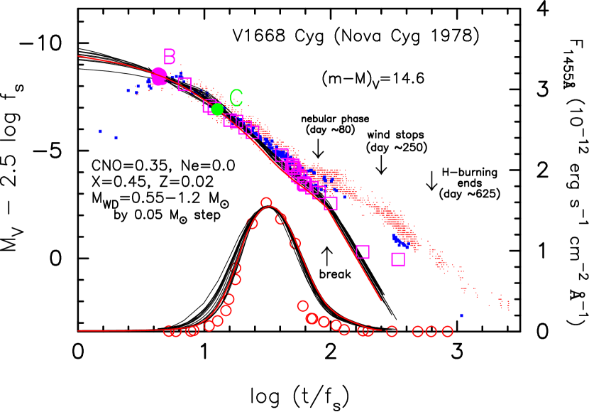
Figure 49: Same as Figure 48, but on a logarithmic timescale. The right edges of free-free emission model light curves correspond to the epoch when the optically thick winds stop. Other characteristic epochs are indicated for V1668 Cyg and the $0.98~{}M_{\sun}$ WD model. The model light curves show a bend $\sim 100$ days after the outburst, which is labeled “break.” This corresponds roughly to the start of the nebular phase of V1668 Cyg.

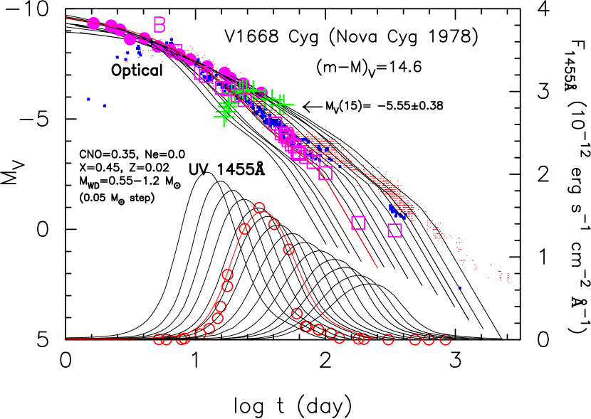
Figure 50: Same as Figure 49, but in the absolute $V$ magnitude vs. logarithmic timescale plane. The position at point B in Figures 48 and 49 is indicated by the filled magenta circle on each $V$ light curve. We also show the absolute magnitude 15 days after the optical maximum, $M_{V}(15)$, by the green crosses. The solid red lines indicate the $0.98~{}M_{\sun}$ WD model for V1668 Cyg.

A.3 Time-stretching method of nova light curves

Hachisu & Kato (2010) proposed a time-stretching method of nova light curves based on the universal decline law, and determined the timescaling factor of $f_{\rm s}$ and distance modulus in the $V$ band, $\mu_{V}\equiv(m-M)_{V}$, for various novae (see also Appendix of Hachisu & Kato, 2016a). In this subsection, we briefly explain how the time-stretching method works.

Figure 49 shows the same free-free emission model light curves of Figure 48, but on a logarithmic timescale, because we manipulate the nova light curves much more easily on logarithmic timescales. Figure 50 shows the same model light curves in Figure 47 but without time-normalization, i.e., $M_{V}$ vs. $\log t$. If we stretch/squeeze these light curves by $f_{\rm s}$ and shift in the vertical direction by $-2.5\log f_{\rm s}$, we obtain Figure 49.

If we pick two light curves in Figure 50 and overlap them by shifting one of the two, horizontally back and forth and vertically up and down, as in Figure 49, we can measure the timescaling factor of $f_{\rm s}$ from the time-shift of $\log f_{\rm s}=\Delta\log t$ and the difference in the absolute $V$ magnitude, $\Delta M_{V}$, from $\Delta M_{V}=-2.5\log f_{\rm s}$ with respect to the other. The stretching factor $f_{\rm s}$ is obtained for a selected nova (target nova) against the other (template nova). If the absolute magnitude of the template nova is known, the absolute magnitude of the target nova is calculated from

$$\left(M_{V}[t]\right)_{\rm template} = \left(M^{\prime}_{V}[t^{\prime}]\right)_{\rm target}$$ (A1)

$$= \left(M_{V}[t/f_{\rm s}]\right)_{\rm target}-2.5\log f_{\rm s},$$ (A2)

where the brightness $(t,~{}M_{V})$ of the target nova is converted to the brightness ($t^{\prime},~{}M^{\prime}_{V}$) by time-stretch $t^{\prime}=t/f_{\rm s}$ and $M^{\prime}_{V}[t^{\prime}]=M_{V}[t/f_{\rm s}]-2.5\log f_{\rm s}$. Here, we note $M_{V}[t]$ to demonstrate that $M_{V}$ is a function of $t$. This relation is easily understood from Figures 49 and 50. This equation is equivalent to

$$\left(M_{V}[t\times f_{\rm s}]\right)_{\rm template} = \left(M^{\prime}_{V}[t]\right)_{\rm target}$$ (A3)

$$= \left(M_{V}[t]\right)_{\rm target}-2.5\log f_{\rm s}.$$ (A4)

Using the inverse time-stretch $t^{\prime}=t\times f_{\rm s}$ and $M^{\prime}_{V}[t^{\prime}]=M_{V}[t\times f_{\rm s}]+2.5\log f_{\rm s}$ for the template, we rewrite Equation (A2) as

$$\left(M_{V}[t]\right)_{\rm target} = \left(M^{\prime}_{V}[t^{\prime}]\right)_{\rm template}$$ (A5)

$$= \left(M_{V}[t\times f_{\rm s}]\right)_{\rm template}+2.5\log f_{\rm s}.$$ (A6)

In general, we obtain nova light curves in the apparent magnitude. The difference between the apparent magnitudes of the two novae is obtained as

$$(m_{V}[t])_{\rm target}=(m_{V}[t\times f_{\rm s}])_{\rm template}+(\Delta V)_{\rm template},$$ (A7)

where we squeezed the apparent $V$ magnitude light curve of the template nova horizontally (in the time direction) by a factor of $f_{\rm s}$ and shifted vertically by $(\Delta V)_{\rm template}$ to overlap with the target nova. Subtracting Equation (A6) from Equation (A7), we obtain the distance modulus of the target nova as

$$\left(m[t]-M[t]\right)_{V,\rm target}=\left((m[t\times f_{\rm s}]-M[t\times f_{\rm s}])_{V}+\Delta V\right)_{\rm template}-2.5\log f_{\rm s}.$$ (A8)

Because $(m[t]-M[t])_{V}$ is a constant, we simply write Equation (A8) as

$$(m-M)_{V,\rm target}=\left((m-M)_{V}+\Delta V\right)_{\rm template}-2.5\log f_{\rm s},$$ (A9)

where $(m-M)_{V,\rm template}$ is the distance modulus of the template nova, which is known. Equation (A9) is the same equation as Equation (11). Thus, we can obtain the distance modulus of a target nova by comparing it with the template nova. Hachisu & Kato (2010) called this method the time-stretching method.

The above mathematical relations are derived from the universal decline law, which is based on the free-free emission model light curves calculated from the optically thick wind model (see Appendices of Hachisu & Kato, 2010, 2016a, for more detail). Note that individual nova light curves more or less deviate from the universal decline law for various reasons but these relations approximately represent the overall trends between nova light curves.

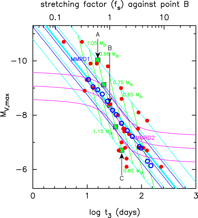
Figure 51: The maximum magnitude vs. rate of decline (MMRD) relation. The ordinate is the absolute $V$ magnitude and the abscissa is the $t_{3}$ time. The open blue circles are the MMRD points calculated from our various WD mass models in Figure 50. Point B represents the peak brightness of V1668 Cyg for a nova model on a $0.98M_{\sun}$ WD with the chemical composition of CO nova 3 (Hachisu & Kato, 2016a). We suppose that B corresponds to a typical initial envelope mass for a nova of a given WD mass. The thick cyan line passing through point B corresponds to a MMRD relation of novae with typical initial envelope mass but different WD mass. The cyan line passing through point A is a MMRD relation for a much larger initial envelope mass than that of point B (much lower mass accretion rates). The cyan line passing through point C is a MMRD relation for a much smaller initial envelope mass than that of point B (much higher mass accretion rates). The green solid lines connect the same WD mass, i.e., 1.15, 1.05, 0.98, 0.85, 0.75, and 0.65 $M_{\sun}$. The filled red circles are MMRD points for individual galactic novae taken from Table 5 of Downes & Duerbeck (2000). The cyan lines envelop these MMRD points studied by Downes & Duerbeck (2000). Two well-known MMRD relations are added: Kaler-Schmidt’s law (Schmidt, 1957) indicated by blue solid lines labeled “MMRD1,” and Della Valle & Livio’s (1995) law indicated by magenta solid lines labeled “MMRD2.” We add upper/lower bounds of $\pm 0.5$ mag for each of these two MMRD relations.

Appendix B Theoretical maximum magnitude vs. rate of decline relations

The Maximum Magnitude vs. Rate of Decline (MMRD) relation, i.e., the relation between $M_{V,{\rm max}}$ and ($t_{2}$ or) $t_{3}$, is often used to estimate the distance to novae (e.g., Cohen, 1988; della Valle & Livio, 1995; de Vaucouleurs, 1978; Downes & Duerbeck, 2000; Schmidt, 1957). The time-stretching method is fundamentally different from the MMRD methods, mainly because the time-stretching method does not require the peak brightness (maximum magnitude). In this subsection, we present a theoretical explanation of the MMRD relations not only on the main trend but also on the large scatter of individual novae around the main trend, based on the time-stretching method. The essential part of the theoretical explanation is given in Figure 15 of Hachisu & Kato (2010), Figure 36 of Hachisu & Kato (2015), and Figures 47 and 48 of Hachisu & Kato (2016a), but here we give a systematic description on the main trend of MMRD relations and scatter around the main trend.

The main trend of MMRD relations can be explained as follows. The model light curves of free-free emission decline along the decreasing envelope mass, $M_{\rm env}$, and thus, the peak brightness depends on the initial envelope mass, $M_{\rm env,0}$, at maximum. In other words, by specifying the WD mass and initial envelope mass, we can determine the peak brightness on the light curve. For example, the peak brightness of V1668 Cyg corresponds to point B in Figures 48 and 49. If we assume that V1668 Cyg has a typical peak brightness, which is expressed by a point (point B) in the $\log(t/f_{\rm s})$-$(M_{V}-2.5\log f_{\rm s})$ plane (Figure 49), other speed classes (other WD masses) of novae have the typical peak brightness $M_{V}$ at point B (filled magenta circles) in the real timescale $\log t$ (Figure 50). This means that a faster declining nova (smaller $t_{2}$ or $t_{3}$ time) has a brighter maximum magnitude (smaller $M_{V,{\rm max}}$) and a slower declining nova has a fainter peak.

We read the value of $M_{V,\rm max}$ at point B (filled magenta circle) on each model light curve (different WD mass) and obtain its $t_{3}$ time in Figure 50. Then, we plot the positions of $(t_{3},~{}M_{V,\rm max})$ by the open blue circles in Figure 51, which are approximately located on the thick straight cyan line. This is the main trend of the MMRD relation. In short, the main trend of the MMRD relation is explained by the difference in the WD mass.

Now, we derive a simple theoretical formula for the MMRD relation based on the universal decline law. Here, we take the absolute $V$ magnitude light curve of the $0.98~{}M_{\sun}$ WD model (solid red lines in Figures 48, 49, and 50) as the representative of the universal decline law. The apparent brightness, $m_{V,{\rm max}}$, at point B of each light curve with different WD masses (different $f_{\rm s}$) is expressed as $m_{V,{\rm max}}=m^{\prime}_{V,{\rm max}}+2.5\log f_{\rm s}$ and $t_{3}=t^{\prime}_{3}\times f_{\rm s}$ by time-stretch. Eliminating $f_{\rm s}$ from these two relations, we have

$$m_{V,{\rm max}}=2.5\log t_{3}+m^{\prime}_{V,{\rm max}}-2.5\log t^{\prime}_{3}.$$ (B1)

Because point B corresponds to the optical peak of V1668 Cyg ($f_{\rm s}=1.0$ in Figure 48), we obtain $t^{\prime}_{3}=26$ days and $m^{\prime}_{V,{\rm max}}=6.2$ from the V1668 Cyg light curve. Substituting $t^{\prime}_{3}=26$ days and $m^{\prime}_{V,{\rm max}}=6.2$ into Equation (B1), we have

$$m_{V,{\rm max}}=2.5\log t_{3}+6.2-2.5\log 26=2.5\log t_{3}+2.7.$$ (B2)

This is our theoretical apparent MMRD relation for a maximum point B in Figure 48. Using the distance modulus of $(m-M)_{V}$, we obtain our theoretical MMRD relation as

$$M_{V,{\rm max}} = m_{V,{\rm max}}-(m-M)_{V}$$ (B3)

$$= 2.5\log t_{3}+m^{\prime}_{V,{\rm max}}-2.5\log t^{\prime}_{3}-(m-M)_{V}.$$ (B4)

Substituting $(m-M)_{V}=14.6$ for V1668 Cyg into Equation (B4), we have

$$M_{V,{\rm max}} = 2.5\log t_{3}+6.2-2.5\log 26-14.6$$ (B5)

$$= 2.5\log t_{3}-11.9.$$ (B6)

Figure 51 shows this theoretical MMRD relation (passing through point B) for novae by the thick solid cyan line. We show the value of $f_{\rm s}$ on the upper horizontal axis of Figure 51, which corresponds to the $t_{3}$ time on the lower horizontal axis.

Next, we explain the reason why individual novae deviate from the main trend of MMRD relation, Equation (B6). If the initial envelope mass, $M_{\rm env,0}$, is larger or smaller than that at point B, we obtain different MMRD relations. Hachisu & Kato (2010) showed that the peak magnitude is brighter for a larger initial envelope mass, even for the same WD mass. Suppose that a nova follows a similar light curve to V1668 Cyg but reaches a much brighter peak, e.g., point A in Figure 48. Figure 48 shows that $t_{3}$ time is smaller for a brighter peak (point A) compared with $t_{3}$ for point B. (See also Figure 2 of Hachisu & Kato (2010) for the same trend of $t_{3}$ time). This corresponds to a different initial envelope mass for the same $0.98~{}M_{\sun}$ WD and chemical composition.

The solid cyan lines passing through points A, B, and C in Figure 51 indicates the degree of deviation from point B, originating from the difference in the peak brightness (i.e., the difference in the initial envelope mass). In other words, novae on the same WD mass show large scatter from the main trend of the thick solid cyan line in both sides of brighter/fainter along the solid green lines of the 1.15, 1.05, 0.98, 0.85, 0.75, and $0.65~{}M_{\sun}$ WD models.

Now we obtain the region that covers the scatter in Figure 51. Point A $(t^{\prime}_{3}=16$ days, $m^{\prime}_{V,{\rm max}}=4.6)$ in Figure 48 corresponds to a larger envelope mass than point B. The solid cyan line passing through point A is

$$M_{V,{\rm max}} = 2.5\log t_{3}+4.6-2.5\log 16-14.6$$ (B7)

$$= 2.5\log t_{3}-13.0,$$ (B8)

from Equation (B4). The solid cyan line passing through point C $(t^{\prime}_{3}=43$ days, $m^{\prime}_{V,{\rm max}}=7.9)$ has a different $t_{3}$–$M_{V,{\rm max}}$ relation for a much smaller initial envelope mass (at point C in Figure 48), i.e.,

$$M_{V,{\rm max}} = 2.5\log t_{3}+7.9-2.5\log 43-14.6$$ (B9)

$$= 2.5\log t_{3}-10.8,$$ (B10)

from Equation (B4). In our theoretical understanding of novae, the smaller the mass accretion rate, the larger the ignition mass. Thus, the envelope mass at the peak, $M_{\rm env,0}$, is larger (see Figure 3 of Kato et al., 2014, for the ignition mass vs. mass accretion rate).

Our theoretical MMRD relation of Equation (B6) is in good agreement with two well-known, empirically obtained MMRD relations, Kaler-Schmidt’s law (MMRD1) in Equation (32) and Della Valle & Livio’s law (MMRD2) in Equation (33). We plot these MMRD relations in Figure 51. Kaler-Schmidt’s law is denoted by the straight blue line with two attendant blue lines, corresponding to $\pm 0.5$ mag brighter/fainter cases. Della Valle & Livio’s law is indicated by the magenta solid lines, also with two attendant magenta lines of $\pm 0.5$ mag. These two well-known empirical MMRD relations are very close to our theoretical MMRD relation.

In Figure 51, we also add observational MMRD points (filled red circles) for individual galactic novae, the data of which are taken from Table 5 of Downes & Duerbeck (2000). It is clearly shown that the large scatter of individual points from the two empirical MMRD relations (blue and magenta lines) falls into between upper/lower cases of our MMRD relations for the largest (point A) and smallest (point C) initial envelope mass of $M_{\rm env,0}$. This simply means that there is a second parameter to specify the MMRD points for individual novae. As explained above, the main parameter is the WD mass, represented by the timescaling factor $f_{\rm s}$. The second parameter is the initial envelope mass (or the mass accretion rate onto the WD). This second parameter can reasonably explain the scatter of individual novae from all the proposed empirical MMRD relations.

References

- Abdo et al. (2010) Abdo, A. A., Ackermann, M., Ajello, M., et al. 2010, Science, 329, 817
- Ackermann et al. (2014) Ackermann, M., Ajello, M., Albert, A., et al. 2014, Science, 345, 554
- Anupama & Dewangan (2000) Anupama, G. C., & Dewangan, G. C. 2000, AJ, 119, 1359
- Anupama et al. (2013) Anupama, G. C., Kamath, U. S., Ramaprakash, A. N., et al. 2013, A&A, 559, A121
- Aydi et al. (2018) Aydi, E., Page, K. L., Kuin, N. P. M., et al. 2018, MNRAS, 474, 2679
- Bailey (1981) Bailey, J. 1981, MNRAS, 197, 31
- Banerjee et al. (2014) Banerjee, D. P. K., Joshi, V., Venkataraman, V., et al. 2014, MNRAS, 785, L11
- Barlow et al. (1981) Barlow, M. J., et al. 1981, MNRAS, 195, 61
- Barry et al. (2008) Barry, R. K., Mukai, K., Sokoloski, J. L., et al. 2008, RS Ophiuchi (2006) and the Recurrent Nova Phenomenon, ASP Conference Series, 401, eds. A. Evans, M. F. Bode, T. J. O’Brien, & M. J. Darnley, San Francisco, Astronomical Society of the Pacific, 52
- Belczyński & Mikołajewska (1998) Belczyński, K., & Mikołajewska, J., 1998, MNRAS, 296, 77
- Bode et al. (2016) Bode, M. F., Darnley, M. J., Beardmore, A. P., et al. 2016, ApJ, 818, 145
- Bond et al. (2004) Bond, H. E., Walter, F., Espinoza, J., et al. 2004, IAU Circ., 8424, 1
- Brandi et al. (2009) Brandi, E., Quiroga, C., Mikołajewska, J., Ferrer, O. E., & García, L. G. 2009, A&A, 497, 815
- Cardelli et al. (1989) Cardelli, J. A., Clayton, G. C., & Mathis, J. S. 1989, ApJ, 345, 245
- Cassatella et al. (2002) Cassatella, A., Altamore, A., & González-Riestra, R. 2002, A&A, 384, 1023
- Cho et al. (2015) Cho, S.-H., Kim, J., Yun, Y. 2015, J. Korean Astr. Society, 48, 267
- Cohen (1988) Cohen, J. G. 1988, The extragalactic distance scale, ASP conference series, 4, 114
- Connelley & Sandage (1958) Connelley, M., & Sandage, A. 1970, PASP, 70, 600
- Darnley et al. (2015) Darnley, M. J., Henze, M., Steele, I.A. et al. 2015, A&A, 580, A45
- Darnley et al. (2016) Darnley, M. J., Henze, M., Bode, M. F. et al. 2016, ApJ, 833, 149
- Darnley et al. (2017) Darnley, M. J., Hounsell, R., Godon, P., et al. 2017, ApJ, 849, 96
- Deguchi et al. (2011) Deguchi, S., Koike, K., Kuno, N., et al. 2011, PASJ, 63, 309
- Denissenkov et al. (2013) Denissenkov, P. A., Herwig, F., Bildsten, L., & Paxton, B. 2013, ApJ, 762, 8
- della Valle & Livio (1995) della Valle, M., & Livio, M. 1995, ApJ, 452, 704
- de Vaucouleurs (1978) de Vaucouleurs, G. 1978, ApJ, 223, 351
- Doherty et al. (2015) Doherty, C. L., Gil-Pons, P., Siess, L., Lattanzio, J. C., & Lau, H. H. B. 2015, MNRAS, 446, 2599
- Downes & Duerbeck (2000) Downes, R. A., & Duerbeck, H. W. 2000, AJ, 120, 2007
- Ennis et al. (1977) Ennis, D., Becklin, E. E., Beckwith, S., et al. 1977, ApJ, 214, 478
- Esipov et al. (2015) Esipov, V. F., Kolotilov, E. A., Shenavrin, V. I., et al. 2015, Baltic Astronomy, 24, 353
- Evans et al. (2009) Evans, P. A., Beardmore, A. P., Page, K. L., et al. 2009, MNRAS, 397, 1177
- Feast et al. (1989) Feast, M. W., Glass, I. S., Whitelock, P. A., & Catchpole, R. M. 1989, MNRAS, 241, 375
- Fekel et al. (2000) Fekel, F. C., Joyce, R. R., Hinkle, K. H., & Skrutskie, M. F. 2000, AJ, 119, 1375
- Gallagher & Ney (1976) Gallagher, J. S., & Ney, E. P. 1976, ApJ, 204, L35
- Gehrz et al. (1980) Gehrz, R. D., Hackwell, J. A., Grasdalen, G. I. et al. 1980, ApJ, 239, 570
- Glass & Feast (1982) Glass, I. S., & Feast, M. W. 1982, MNRAS, 199, 245
- Green et al. (2015) Green, G. M., Schlafly, E. F., Finkbeiner, D. P., et al. 2015, ApJ, 810, 25
- Green et al. (2018) Green, G. M., Schlafly, E. F., Finkbeiner, D. P., et al. 2018, arXiv:1801.03555
- Güver & Özel (2009) Güver, T., & Özel, F. 2009, MNRAS, 400, 2050
- Hachisu & Kato (2001b) Hachisu, I., & Kato, M. 2001b, ApJ, 558, 323
- Hachisu & Kato (2003) Hachisu, I., & Kato, M. 2003, ApJ, 588, 1003
- Hachisu & Kato (2006) Hachisu, I., & Kato, M. 2006, ApJS, 167, 59
- Hachisu & Kato (2007) Hachisu, I., & Kato, M. 2007, ApJ, 662, 552
- Hachisu & Kato (2009) Hachisu, I., & Kato, M. 2009, ApJ, 694, L103
- Hachisu & Kato (2010) Hachisu, I., & Kato, M. 2010, ApJ, 709, 680
- Hachisu & Kato (2012) Hachisu, I., & Kato, M. 2012, Baltic Astronomy, 21, 68
- Hachisu & Kato (2014) Hachisu, I., & Kato, M. 2014, ApJ, 785, 97
- Hachisu & Kato (2015) Hachisu, I., & Kato, M. 2015, ApJ, 798, 76
- Hachisu & Kato (2016a) Hachisu, I., & Kato, M. 2016a, ApJ, 816, 26
- Hachisu & Kato (2016b) Hachisu, I., & Kato, M. 2016b, ApJS, 223, 21
- Hachisu et al. (2008b) Hachisu, I., Kato, M., & Cassatella, A. 2008b, ApJ, 687, 1236
- Hachisu et al. (2000a) Hachisu, I., Kato, M., Kato, T., & Matsumoto, K. 2000a, ApJ, 528, L97
- Hachisu et al. (2000b) Hachisu, I., Kato, M., Kato, T., Matsumoto, K., & Nomoto, K. 2000b, ApJ, 534, L189
- Hachisu et al. (2006b) Hachisu, I., Kato, M., Kiyota, S., et al. 2006b, ApJ, 651, L141
- Hachisu et al. (2007) Hachisu, I., Kato, M., & Luna, G. J. M. 2007, ApJ, 659, L153
- Hachisu et al. (1999a) Hachisu, I., Kato, M., & Nomoto, K. 1999a, ApJ, 522, 487
- Hachisu et al. (2008a) Hachisu, I., Kato, M., & Nomoto, K. 2008a, ApJ, 683, L127
- Hachisu et al. (2012) Hachisu, I., Kato, M., & Nomoto, K. 2012, ApJ, 756, L4
- Hachisu et al. (1999b) Hachisu, I., Kato, M., Nomoto, K., & Umeda, H. 1999b, ApJ, 519, 314
- Hachisu et al. (2003) Hachisu, I., Kato, M., & Schaefer, B. E. 2003, ApJ, 584, 1008
- Harrison et al. (1993) Harrison, T. E., Johnson, J. J., & Spyromilio, J. 1993, AJ, 105, 320
- Harrison et al. (1994) Harrison, T. E., & Stringfellow, G. S. 1994, ApJ, 437, 827
- Henze et al. (2015) Henze, M., Ness, J.-U., Darnley, M., et al. 2015, A&A, 580, A46,
- Hjellming et al. (1986) Hjellming, R. M., van Gorkom, J. H., Seaquist, E. R., et al. ApJ, 305, L71
- Hoard et al. (2002) Hoard, D. W., Wachter, S., Clark, L. Lee, & Bowers, T. P. 2002, ApJ, 565, 511
- Hounsell et al. (2010) Hounsell, R., Bode, M. F., Hick, P. P., et al. 2010, ApJ, 724, 480
- Iijima (2009) Iijima, T. 2009, A&A, 505, 287
- Iijima (2015) Iijima, T. 2015, AJ, 150, 20
- Imara & Blitz (2007) Imara, N., & Blitz, L. 2007, ApJ, 662, 969
- Ingram et al. (1992) Ingram, D., Garnavich, P., Green, P., & Szkody, P. 1992, PASP, 104, 402
- Ita & Matsunaga (2011) Ita, Y., & Matsunaga, N. 2011, MNRAS, 412, 2345
- Jablonski & Oliveira (2016) Jablonski, F., & Oliveira, A. 2016, ATel, 9684, 1
- Joshi et al. (2015) Joshi, V., Banerjee, D. P. K., Ashok, N. M., Venkataraman, V., & Walter, F. M. 2015, MNRAS, 452, 3696
- Kantharia et al. (2016) Kantharia, N. G., Dutta, P., Roy, N. 2016, MNRAS, 456, L49
- Kasliwal et al. (2011) Kasliwal, M. M., Cenko, S. B., Kulkarni, S. R., et al. 2011, ApJ, 735, 94
- Kato & Hachisu (1994) Kato, M., & Hachisu, I., 1994, ApJ, 437, 802
- Kato & Hachisu (2012) Kato, M., & Hachisu, I., 2012, Bull. Astr. Soc. India, 40, 393
- Kato et al. (2009) Kato, M., Hachisu, I., & Cassatella, A. 2009, ApJ, 704, 1676
- Kato et al. (2014) Kato, M., Saio, H., Hachisu, I., & Nomoto, K. 2014, ApJ, 793, 136
- Kato et al. (2017) Kato, M., Hachisu, I., & Saio, H. 2017, arXiv:1701.01825
- Kato et al. (2015) Kato, M., Saio, H., & Hachisu, I. 2015, ApJ, 808, 52
- Kato et al. (2016) Kato, M., Saio, H., Henze, M., et al. 2016, ApJ, 830, 40
- Kato et al. (2017) Kato, M., Saio, H., & Hachisu, I. 2017, ApJ, 838, 153
- Klare et al. (1980) Klare, G., Wolf, B., & Krautter, J. 1980, A&A, 89, 282
- Kobayashi et al. (1998) Kobayashi, C., Tsujimoto, T., Nomoto, K., Hachisu, I., & Kato, M. 1998, ApJ, 503, L155
- Kolotilov et al. (1998) Kolotilov, E. A., Munari, U., Popova, A. A., et al. 1998, Astronomy Letters, 24, 451
- Kolotilov et al. (2003) Kolotilov, E. A., Shenavrin, V. I., Shugarov, S. Yu., & Yudin, B. F. 2003, Astronomy Reports, 47, 777
- Leibowitz et al. (1992) Leibowitz, E., Mendelson, H., Mashal, E., Prialnik, D., & Seitter, W. C. 1992, ApJ, 385, L49
- Liller (2009) Liller, W. 2009, IAU Circ., 9019, 1
- Liller et al. (2004) Liller, W., Pearce, A., & Monard, L. A. G. 2004, IAU Circ., 8422, 1
- Lipunov et al. (2016) Lipunov, V., Podesta, R., Levato, H., et al. 2016, ATel, 9631, 1
- Liszt (2014) Liszt, H. S. 2014, ApJ, 780, 10
- Lynch et al. (1992) Lynch, D. K., Hackwell, J. A., & Russell, R. W. 1992, ApJ, 398, 632
- Maoz et al. (2014) Maoz, D., Mannucci, F., & Nelemans, G. 2014, ARA&A, 52, 107
- Marshall et al. (2006) Marshall, D. J., Robin, A. C., Reylé, C., Schultheis, M., & Picaud, S. 2006, A&A, 453, 635
- Mason et al. (2012) Mason, E., Ederoclite, A., Williams, R. E., Della Valle, M., Setiawan, J. 2012, A&A, 544, A149
- Mason & Munari (2014) Mason, E., & Munari, U. 2014, A&A, 569, A84
- Matheson et al. (1993) Matheson, T., Filippenko, A. V., & Ho, L. C. 1993, ApJ, 418, L29
- Maxwell et al. (2012) Maxwell, M. P., Rushton, M. T., Darnley, M. J., et al. 2013, MNRAS, 419, 1465
- Mennickent & Honeycutt (1995) Mennickent, R. E., & Honeycutt, R. K. 1995, Inf. Bull. Variable Stars, 4232
- Mikołajewska & Shara (2017) Mikołajewska, J., & Shara, M. M. 2017, ApJ, 847, 99
- Mohamed & Podsiadlowski (2012) Mohamed, S., & Podsiadlowski, Ph. 2012, Baltic Astronomy, 21, 88
- Monnier et al. (2006) Monnier, J. D., Barry, R. K., Traub, W. A., et al. 2006, ApJ, 647, L127
- Morris et al. (2017) Morris, P. J., Cotter, G., Brown, A. M., & Chadwick, P. M. 2017, MNRAS, 465, 1218
- Moriya et al. (2013) Moriya, T. J., Maeda, K., Taddia, F., et al. 2013, MNRAS, 435, 1520
- Mróz et al. (2014) Mróz, P., Poleski, R., Udalski, A., et al. 2014, MNRAS, 443, 784
- Mróz et al. (2015) Mróz, P., Udalski, A., Poleski, R., et al. 2015, ApJS, 219, 26
- Mróz et al. (2016) Mróz, P., Udalski, A., Poleski, R., et al. 2016, ApJS, 222, 9
- Munari & Banerjee (2018) Munari, U., & Banerjee, D. P. K. 2018, MNRAS, 475, 508
- Munari et al. (2017) Munari, U., Hambsch, F.-J., & Frigo, A. 2017, MNRAS, 469, 4341
- Munari et al. (2011b) Munari, U., Joshi, V. H., Ashok, N. M., et al. 2011b, MNRAS, 410, L52
- Munari et al. (1990) Munari, U., Margoni, R., & Stagni, R. 1990, MNRAS, 242, 653
- Mürset & Schmid (1999) Mürset, U., & Schmid, H. M. 1999, A&AS, 137, 473
- Nariai et al. (1980) Nariai, K., Nomoto, K., & Sugimoto, D. 1980, PASJ, 32, 473
- Nelson et al. (2012) Nelson, T., Donato, D., Mukai, K., Sokoloski, J., & Chomiuk, L. 2012, ApJ, 748, 43,
- Ness et al. (2007) Ness, J.-U., Schwarz, G. J., Retter, A., et al. 2007, ApJ, 663, 505
- Nishiyama et al. (2010) Nishiyama, K., Kabashima, F., Kojima, T., et al. 2010, IAU Circ., 9130, 1
- Nomoto (1982) Nomoto, K. 1982, ApJ, 253, 798
- Nomoto et al. (2007) Nomoto, K., Saio, H., Kato, M., & Hachisu, I. 2007, ApJ, 663, 1269
- O’Brien et al. (2006) O’Brien, T. J., Bode, M. F., Porcas, R. W., et al. 2006, Nature, 442, 279
- Orio et al. (2015) Orio, M., Rana, V., Page, K. L., Sokoloski, J., Harrison, F. 2015, MNRAS, 448, L35
- Orlando & Drake (2012) Orlando, S., & Drake, J. J. 2012, MNRAS, 419, 2329
- Özdörmez et al. (2016) Özdörmez, A., Güver, T., Cabrera-Lavers, A., Ak, T. 2016, MNRAS, 461, 1177
- Page et al. (2015) Page, K. L., Osborne, J. P., Kuin, N. P. M., et al. 2015, MNRAS, 454, 3108
- Pagnotta & Schaefer (2014) Pagnotta, A., & Schaefer, B. E. 2014, ApJ, 788, 164
- Pagnotta et al. (2015) Pagnotta, A., Schaefer, B. E., Clem, J. L., et al. 2015, ApJ, 811, 32
- Pan et al. (2015) Pan, K.-C., Ricker, P. M., & Taam, R. E. 2015, ApJ, 806, 27
- Perlmutter et al. (1999) Perlmutter, S., Aldering, G., Goldhaber, G. et al. 1999, ApJ, 517, 565
- Phillips (1993) Phillips, M. M. 1993, ApJ, 413, L105
- Piatti & Geisler (2013) Piatti, A., & Geisler, D. 2013 AJ, 145, 17
- Pietrzyński et al. (2013) Pietrzyński, G., Graczyk, D., Gieren, W., et al. 2011, Nature, 495, 76
- Prialnik (1986) Prialnik, D. 1986, ApJ, 310, 222
- Rieke & Lebofsky (1985) Rieke, G. H., & Lebofsky, M. J. 1985, ApJ, 288, 618
- Riess et al. (1998) Riess, A. G., Fillipenko, A. V., Challis, P. et al. 1998, AJ, 116, 1009
- Sala & Hernanz (2005) Sala, G., & Hernanz, M. 2005, A&A, 439, 1061
- Schaefer (2009) Schaefer, B. E. 2009, ApJ, 697, 721
- Schaefer (2010) Schaefer, B. E. 2010, ApJS, 187, 275
- Schaefer (2011) Schaefer, B. E. 2011, ApJ, 742, 112
- Schaefer & Ringwald (1995) Schaefer, B. E., & Ringwald, F. A. 1995, ApJ, 447, L45
- Schaefer et al. (2011) Schaefer, B. E., Pagnotta, A., LaCluyze, A. P., et al. 2011, ApJ, 742, 113
- Shafter (2013) Shafter, A. W. 2013, AJ, 145, 117
- Schlafly & Finkbeiner (2011) Schlafly, E. F., & Finkbeiner, D. P. 2011, ApJ, 737, 103
- Schmidt (1957) Schmidt, Th. 1957, Z. Astrophys., 41, 181
- Schwarz et al. (2007) Schwarz, G. J., Shore, S. N., Starrfield, S., Vanlandingham, K. M. 2007, ApJ, 657, 453
- Schwarz et al. (2011) Schwarz, G. J., Ness, J.-U., Osborne, J. P., et al. 2011, ApJS, 197, 31
- Schwarz et al. (2015) Schwarz, G. J., Shore, S. N., Page, K. L., et al. 2015, AJ, 149, 95
- Seach et al. (2012) Seach, J., Liller, W., Brimacombe, J., & Pearce, A. 2012, CBET, 3071, 1
- Seaton (1979) Seaton, M. J. 1979, MNRAS, 187, 73
- Sekiguchi et al. (1988) Sekiguchi, K., Feast, M. W., Whitelock, P. A., et al. 1988, MNRAS, 234, 281
- Sekiguchi et al. (1990) Sekiguchi, K., Whitelock, P. A., Feast, M. W., et al. 1990, MNRAS, 246, 78
- Shara et al. (2017) Shara, M. M., Doyle, T., Lauer, T. R., et al. 2017, ApJ, 839, 109
- Shore et al. (2011) Shore, S. N., Wahlgren, G. M., Augusteijn, T., et al. 2011, A&A, 527, A98
- Shumkov et al. (2016) Shumkov, V., Lipunov, V., Podesta, R., et al. 2016, ATel, 9621, 1
- Siviero & Munari (2006) Siviero, A., & Munari, U. 2006, CBET, 502, 1
- Snijders (1987) Snijders, M. A. J. 1987, Ap&SS, 130, 243
- Sokoloski et al. (2013) Sokoloski, J. L., Crotts, A. P. S., Lawrence, S., & Uthas, H. 2013, ApJ, 770, L33
- Sokoloski et al. (2006) Sokoloski, J. L., Luna, G. J. M., Mukai, K., & Kenyon, S. J. 2006, Nature, 442, 276
- Sostero & Guido (2006a) Sostero, G., & Guido, E. 2006a, IAU Circ., 8673, 3
- Sostero & Guido (2006b) Sostero, G., & Guido, E. 2006b, IAU Circ., 8681, 4
- Sostero et al. (2006c) Sostero, G., Guido, E., & West, J. D. 2006c, CBET, 502, 2
- Starrfield et al. (1972) Starrfield, S., Truran, J. W.., Sparks, W. M., & Kutter, G. S. 1972, ApJ, 176, 169
- Starrfield et al. (1992) Starrfield, S., Shore, S. N., Sparks, W. M., et al. 1992, ApJ, 391, L71
- Strope et al. (2010) Strope, R., Schaefer, B. E., & Henden, A. A. 2010, AJ, 140, 34
- Thoroughgood et al. (2001) Thoroughgood, T. D., Dhillon, V. S., Littlefair, S. P., Marsh, T. R., & Smith, D. A. 2001, MNRAS, 327, 1323
- van den Bergh & Younger (1987) van den Bergh, S., & Younger, P. F. 1987, A&AS, 70, 125
- Vanlandingham et al. (1996) Vanlandingham, K. M., Starrfield, S., Wagner, R. M., Shore, S. N., & Sonneborn, G. 1996, MNRAS, 282, 563
- Vanlandingham et al. (1997) Vanlandingham, K. M., Starrfield, S., & Shore, S. N. 1997, MNRAS, 290, 87
- Walter et al. (2012) Walter, F. M., Battisti, A., Towers, S. E., Bond, H. E., & Stringfellow, G. S. 2012, PASP, 124, 1057
- Whitelock et al. (2008) Whitelock, P. A., Feast, M. W., & van Leeuwen, F. 2008, MNRAS, 386, 313
- Williams et al. (1994) Williams, R. E., Phillips, M. M., & Hamuy, M. 1994, ApJS, 90, 297
- Woodward et al. (1992) Woodward, C. E., Gehrz, R. D., Jones, T. J., & Lawrence, G. F. 1992, ApJ, 384, L41
- Woodward et al. (1997) Woodward, C. E., Gehrz, R. D., Jones, T. J., Lawrence, G. F., & Skrutskie, M. F. 1997, ApJ, 477, 817
- Wu et al. (2017) Wu, C., Wang, B., Liu, D., & Han, Z. 2017, A&A, 604, A31