A multipoint stress mixed finite element method for elasticity on simplicial grids

Abstract

We develop a new multipoint stress mixed finite element method for linear elasticity with weakly enforced stress symmetry on simplicial grids. Motivated by the multipoint flux mixed finite element method for Darcy flow, the method utilizes the lowest order Brezzi-Douglas-Marini finite element spaces for the stress and the vertex quadrature rule in order to localize the interaction of degrees of freedom. This allows for local stress elimination around each vertex. We develop two variants of the method. The first uses a piecewise constant rotation and results in a cell-centered system for displacement and rotation. The second uses a piecewise linear rotation and a quadrature rule for the asymmetry bilinear form. This allows for further elimination of the rotation, resulting in a cell-centered system for the displacement only. Stability and error analysis is performed for both variants. First-order convergence is established for all variables in their natural norms. A duality argument is further employed to prove second order superconvergence of the displacement at the cell centers. Numerical results are presented in confirmation of the theory.

1 Introduction

Mixed finite element (MFE) methods for elasticity with stress-displacement formulations provide accurate stress, local momentum conservation, and robust treatment of almost incompressible materials. Numerous methods with strong stress symmetry [11, 6, 15] and weak stress symmetry [9, 47, 10, 16, 22, 31, 7, 13, 38] have been developed. A drawback of these methods is that the resulting algebraic systems are of saddle point type. Two common approaches for reducing MFE formulations to positive definite systems include hybridization, resulting in skeletal systems, and reduction to cell-centered systems. In the context of stress-displacement elasticity formulations, hybridization is possible for non-conforming MFE methods [12, 8, 30] or hybridizable discontinuous Galerkin (HDG) methods [23, 43]. These methods require facet displacement degrees of freedom corresponding to polynomials of at least first order.

In this paper we develop MFE methods for elasticity on simplicial grids that can be reduced to symmetric and positive definite cell centered systems based on piecewise constant approximations. These methods have reduced computational complexity compared to hybrid formulations, both due to the smaller polynomial degree and the fact that there are fewer elements than facets. Our approach is motivated by the multipoint flux mixed finite element (MFMFE) method [50, 35, 49] for Darcy flow, which is closely related to the multipoint flux approximation (MPFA) method [1, 2, 27, 28, 3]. The MPFA method is a finite volume method obtained by eliminating fluxes around mesh vertices in terms of neighboring pressures. It can handle discontinuous full tensor coefficients and general grids, thus improving on previously developed cell centered finite difference methods resulting from MFE methods [45, 5, 4], which work for smooth grids and/or coefficients. The MFMFE method [50, 35] utilizes the lowest order Brezzi-Douglas-Marini $\mathcal{BDM}_{1}$ spaces [18] on simplicial and quadrilateral grids, see also a similar approach in [20] on simplices, as well as an enhanced Brezzi-Douglas-Duran-Fortin $\mathcal{BDDF}_{1}$ space [19] on hexahedra. An alternative formulation based on a broken Raviart-Thomas velocity space is developed in [37]. A common feature of the above mentioned methods is that the velocity space has only degrees of freedom that are normal components of the vector on the element boundary, such that on any facet (edge or face) there is one normal velocity associated with each of the vertices. An application of the vertex quadrature rule for the velocity bilinear form results in localizing the interaction of velocity degrees of freedom around mesh vertices. The fluxes then can be locally eliminated, resulting in a cell centered pressure system. The variational framework of the MFMFE methods allows for combining MFE techniques with quadrature error analysis to establish stability and convergence results.

In [41], the multipoint stress approximation (MPSA) method for elasticity was developed, which is a displacement finite volume method based on local stress elimination around vertices in a manner similar to the MPFA method. The method does not have a mixed finite element interpretation, but its stress degrees of freedom correspond to the $\mathcal{BDM}_{1}$ degrees of freedom. The MPSA method was analyzed in [42] by being related to a non-symmetric discontinuous Galerkin (DG) method. A weak symmetry MPSA method has been developed in [36].

In this paper we develop two stress-displacement MFE methods for elasticity on simplicial grids that reduce to cell centered systems. We consider the formulation with weakly imposed stress symmetry, for which there exist MFE spaces with $\mathcal{BDM}_{1}$ degrees of freedom for the stress and piecewise constant displacement. In this formulation the symmetry of the stress is imposed weakly using a Lagrange multiplier, which is a skew-symmetric matrix and has a physical meaning of rotation. Our first method is based on the Arnold-Falk-Winther (AFW) spaces [10] $\mathcal{BDM}_{1}\times\mathcal{P}_{0}\times\mathcal{P}_{0}$, i.e., $\mathcal{BDM}_{1}$ stress and piecewise constant displacement and rotation. Since in $\mathbb{R}^{d}$ there are $d$ normal stress vector degrees of freedom per facet, one degree of freedom can be associated with each vertex, We employ the vertex quadrature rule for the stress bilinear form, which localizes the stress degrees of freedom interaction around vertices, resulting in a block-diagonal stress matrix. This approach resembles the well-known mass-lumping procedure. The stress is then locally eliminated and the method is reduced to a symmetric and positive definite cell centered system for the displacement and rotation. This system is smaller and easier to solve than the original saddle point problem, but no further reduction is possible. Our second method is based on the modified AFW triple $\mathcal{BDM}_{1}\times\mathcal{P}_{0}\times\mathcal{P}_{1}$ proposed in [15]. The difference from the first method is that the rotation is continuous piecewise linear. In this method we employ the vertex quadrature rule both for the stress and the asymmetry bilinear forms. This allows for further local elimination of the rotation after the initial stress elimination, resulting in a symmetric and positive definite cell centered system for the displacement only. This is a very efficient method with computational cost comparable to the MPSA method. Adopting the MPSA terminology, we call our method a multipoint stress mixed finite element (MSMFE) method, with the two variants referred to as MSMFE-0 and MSMFE-1, where the number corresponds to the rotation polynomial degree.

We note that the MSMFE methods inherit the locking-free property of stress-displacement MFE methods for elasticity. A numerical example illustrating the robustness of the MSMFE methods for nearly-incompressible materials is presented in the numerical section. We should mention that a number of locking-free primal-formulation methods have also been developed, including DG [44], a hybrid high order method [24], finite element methods with the Crouzeix-Raviart space [17, 26, 33], weak Galerkin methods [48], a virtual element method [14], and a hybrid finite volume method [25]. These methods have been developed on general polygonal grids, and many of them can have arbitrary order of approximation. However, they require postprocessing for computing the stress and do not provide local equilibrium with $H(\operatorname{div})$-conforming stress.

We perform stability and error analysis for both MSMFE methods. The stability analysis follows the framework established in previous works on MFE methods for elasticity with weak stress symmetry [10, 7], and utilizes the classical Babuška-Brezzi conditions [19]. While the stability of the MSMFE-0 method is relatively straightforward, the analysis of the MSMFE-1 method is not. It requires establishing an inf-sup condition for the Taylor-Hood Stokes pair with vertex quadrature in the divergence bilinear form. We do this by employing a macroelement argument, following an approach developed in [46]. We note that our analysis differs from the one in [46]. In particular, the application of the vertex quadrature rule leads to additional technical difficulties in the inf-sup analysis, since the control of the pressure degrees of freedom by the velocity in the divergence bilinear form is weakened. We proceed with establishing first order convergence for the stress in the $H(\operatorname{div})$-norm and for the displacement and rotation in the $L^{2}$-norm for both methods. The arguments combine techniques from MFE analysis and quadrature error analysis. A duality argument is further employed to prove second order superconvergence of the displacement at the cell centers.

The rest of the paper is organized as follows. The model problem and its MFE approximation are presented in Section 2. The two methods are developed and their stability is analyzed in Sections 3 and 4, respectively. Section 5 is devoted to the error analysis. Numerical results are presented in Section 6.

2 Model problem and its MFE approximation

In this section we recall the weak stress symmetry formulation of the elasticity system. We then present its MFE approximation and a quadrature rule, which form the basis for the MSMFE methods presented in the next sections.

Let $\Omega$ be a simply connected bounded domain of $\mathbb{R}^{d},\,d=2,3$ occupied by a linearly elastic body. We write $\mathbb{M}$, $\mathbb{S}$ and $\mathbb{N}$ for the spaces of $d\times d$ matrices, symmetric matrices and skew-symmetric matrices, all over the field of real numbers, respectively. The material properties are described at each point $x\in\Omega$ by a compliance tensor $A=A(x)$, which is a symmetric, bounded and uniformly positive definite linear operator acting from $\mathbb{S}$ to $\mathbb{S}$. We also assume that an extension of $A$ to an operator $\mathbb{M}\to\mathbb{M}$ still possesses the above properties. As an example, in the case of a homogeneous and isotropic body,

$$A\sigma=\frac{1}{2\mu}\left(\sigma-\frac{\lambda}{2\mu+d\lambda}\operatorname{tr}(\sigma)I\right),$$

where $I$ is the $d\times d$ identity matrix and $\mu>0$, $\lambda>-2\mu/d$ are the Lamé coefficients.

Throughout the paper the divergence operator is the usual divergence for vector fields. When applied to a matrix field, it produces a vector field by taking the divergence of each row. We will also use the curl operator which is the usual curl when applied to vector fields in three dimensions, and it is defined as

$$\operatorname{curl}{\phi}=(\partial_{2}\phi,-\partial_{1}\phi)$$

for a scalar function $\phi$ in two dimensions. Consequently, for a vector field in two dimensions or a matrix field in three dimensions, the curl operator produces a matrix field, by acting row-wise.

Throughout the paper, $C$ denotes a generic positive constant that is independent of the discretization parameter $h$. We will also use the following standard notation. For a domain $G\subset\mathbb{R}^{d}$, the $L^{2}(G)$ inner product and norm for scalar and vector valued functions are denoted $\left(\cdot,\cdot\right)_{G}$ and $\|\cdot\|_{G}$, respectively. The norms and seminorms of the Sobolev spaces $W^{k,p}(G),\,k\in\mathbb{R},p>0$ are denoted by $\|\cdot\|_{k,p,G}$ and $|\cdot|_{k,p,G}$, respectively. The norms and seminorms of the Hilbert spaces $H^{k}(G)$ are denoted by $\|\cdot\|_{k,G}$ and $|\cdot|_{k,G}$, respectively. We omit $G$ in the subscript if $G=\Omega$. For a section of the domain or element boundary $S\subset\mathbb{R}^{d-1}$ we write $\langle\cdot,\cdot\rangle_{S}$ and $\|\cdot\|_{S}$ for the $L^{2}(S)$ inner product (or duality pairing) and norm, respectively. We will also use the spaces

$$H(\operatorname{div};\Omega)=\{v\in L^{2}(\Omega,\mathbb{R}^{d}):\operatorname{div}v\in L^{2}(\Omega)\},$$

$$H(\operatorname{div};\Omega,\mathbb{M})=\{\tau\in L^{2}(\Omega,\mathbb{M}):\operatorname{div}\tau\in L^{2}(\Omega,\mathbb{R}^{d})\},$$

equipped with the norm

$$\|\tau\|_{\operatorname{div}}=\left(\|\tau\|^{2}+\|\operatorname{div}\tau\|^{2}\right)^{1/2}.$$

Given a vector field $f$ on $\Omega$ representing body forces, equations of static elasticity in Hellinger-Reissner form determine the stress $\sigma$ and the displacement $u$ satisfying the constitutive and equilibrium equations respectively:

$$A\sigma=\epsilon(u),\quad\operatorname{div}\sigma=f\quad\text{in }\Omega,$$ (2.1)

together with the boundary conditions

$$u=g\ \text{ on }\Gamma_{D},\quad\sigma\,n=0\ \text{ on }\Gamma_{N},$$ (2.2)

where $\epsilon(u)=\frac{1}{2}\left(\nabla u+(\nabla u)^{T}\right)$ and $\partial\Omega=\Gamma_{D}\cup\Gamma_{N}$. We assume for simplicity that $\Gamma_{D}\neq\emptyset$.

Introducing the Lagrange multiplier $\gamma=\operatorname{Skew}(\nabla u)$, $\operatorname{Skew}(\tau)=\frac{1}{2}(\tau-\tau^{T})$, from the space of skew-symmetric matrices to penalize the asymmetry of the stress tensor, and using that $A\sigma=\nabla u-\gamma$, we arrive at the weak formulation for (2.1)-(2.2), see for example [10, 9]: find $(\sigma,u,\gamma)\in\mathbb{X}\times V\times\mathbb{W}$ such that

$$\begin{aligned} \left(A\sigma,\tau\right)+\left(u,\operatorname{div}\tau\right)+\left(\gamma,\tau\right)&=\langle g,\tau\,n\rangle_{\Gamma_{D}},&\forall\tau&\in\mathbb{X},\\ \left(\operatorname{div}\sigma,v\right)&=\left(f,v\right),&\forall v&\in V,\\ \left(\sigma,\xi\right)&=0,&\forall\xi&\in\mathbb{W},\end{aligned}$$ (2.3)

where the spaces are

$$\mathbb{X}=\big{\{}\tau\in H(\operatorname{div};\Omega,\mathbb{M}):\tau\,n=0\text{ on }\Gamma_{N}\big{\}},\quad V=L^{2}(\Omega,\mathbb{R}^{d}),\quad\mathbb{W}=L^{2}(\Omega,\mathbb{N}).$$

Define the asymmetry operator $\operatorname{as\,}:\mathbb{M}\to\mathbb{R}^{d(d-1)/2}$ such that

$$\operatorname{as\,}(\tau)=\tau_{12}-\tau_{21}\mbox{ in 2D}\,\,\mbox{ and }\operatorname{as\,}(\tau)=(\tau_{32}-\tau_{23},\tau_{31}-\tau_{13},\tau_{21}-\tau_{12})^{T}\mbox{ in 3D}.$$

Let

$$\mathbb{H}=\left\{\begin{array}[]{l}\mathbb{R}^{2},\,d=2,\\ \mathbb{M},\,d=3,\end{array}\right.$$

and define the invertible operators $S:\mathbb{H}\to\mathbb{H}$ and $\Xi:\mathbb{R}^{d(d-1)/2}\to\mathbb{N}$ as follows,

$$\begin{aligned} &d=2:&&S(w)=w\quad\mbox{for }w\in\mathbb{R}^{2},&&\Xi(p)=\begin{pmatrix}0&p\\ -p&0\end{pmatrix}\quad\mbox{for }p\in\mathbb{R},\\ &d=3:&&S(w)=\operatorname{tr\,}(w)I-w^{T}\quad\mbox{for }w\in\mathbb{M},&&\Xi(p)=\begin{pmatrix}0&-p_{3}&p_{2}\\ p_{3}&0&-p_{1}\\ -p_{2}&p_{1}&0\end{pmatrix}\quad\mbox{for }p\in\mathbb{R}^{3}.\end{aligned}$$ (2.4)

A direct calculation shows that for all $w\in\mathbb{H}$,

$$\quad\operatorname{as\,}(\operatorname{curl}(w))=-\operatorname{div}S(w),$$ (2.5)

and for all $\tau\in\mathbb{M}$ and $\xi\in\mathbb{N}$,

$$\left(\tau,\xi\right)=\left(\operatorname{as\,}(\tau),\Xi^{-1}(\xi)\right).$$ (2.6)

2.1 Mixed finite element method

Here we present the MFE approximation of (2.3), which is the basis for the MSMFE methods. Assume for simplicity that $\Omega$ is a polygonal domain and let $\mathcal{T}_{h}$ be a shape-regular and quasi-uniform finite element partition of $\Omega$ [21] consisting of triangles in two dimensions or tetrahedra in three dimensions with maximum diameter $h$. For any element $E\in\mathcal{T}_{h}$ there exists a bijection mapping $F_{E}:\hat{E}\to E$, where $\hat{E}$ is a reference element. Denote the Jacobian matrix by $DF_{E}$ and let $J_{E}=|\operatorname{det}(DF_{E})|$. In the case of triangular meshes, $\hat{E}$ is the reference right triangle with vertices $\hat{\mathbf{r}}_{1}=(0,0^{T})$, $\hat{\mathbf{r}}_{2}=(1,0)^{T}$ and $\hat{\mathbf{r}}_{3}=(0,1)^{T}$. Let $\mathbf{r}_{1}$, $\mathbf{r}_{2}$ and $\mathbf{r}_{3}$ be the corresponding vertices of $E$, oriented counterclockwise. In this case $F_{E}$ is a linear mapping of the form $F_{E}(\hat{\mathbf{r}})=\mathbf{r}_{1}(1-\hat{x}-\hat{y})+\mathbf{r}_{2}\hat{x}+\mathbf{r}_{3}\hat{y}$ with a constant Jacobian matrix and determinant given by $DF_{E}=[\mathbf{r}_{21},\mathbf{r}_{31}]^{T}$ and $J_{E}=2|E|$, where $\mathbf{r}_{ij}=\mathbf{r}_{i}-\mathbf{r}_{j}$. The mapping for tetrahedra is described similarly.

Figure 1: $\mathcal{BDM}_{1}\times\mathcal{P}_{0}\times\mathcal{P}_{0}$ on triangles (left) and $\mathcal{BDM}_{1}\times\mathcal{P}_{0}\times\mathcal{P}_{1}$ on tetrahedra (right).

The finite element spaces $\mathbb{X}_{h}\times V_{h}\times\mathbb{W}_{h}^{k}\subset\mathbb{X}\times V\times\mathbb{W}$ are the triple $\left(\mathcal{BDM}_{1}\right)^{d}\times\left(\mathcal{P}_{0}\right)^{d}\times\left(\mathcal{P}_{k}\right)^{d\times d,skew}$, where $k=0,1$. Note that for $k=1$ the space $\mathbb{W}_{h}^{1}$ contains continuous piecewise linears. On the reference triangle these spaces are defined as

$$\hat{\mathbb{X}}(\hat{E})=\mathcal{P}_{1}(\hat{E})^{2}\times\mathcal{P}_{1}(\hat{E})^{2}=\begin{pmatrix}\alpha_{1}\hat{x}+\beta_{1}\hat{y}+\gamma_{1}&\alpha_{2}\hat{x}+\beta_{2}\hat{y}+\gamma_{2}\\ \alpha_{3}\hat{x}+\beta_{3}\hat{y}+\gamma_{3}&\alpha_{4}\hat{x}+\beta_{4}\hat{y}+\gamma_{4}\end{pmatrix},$$

$$\hat{V}(\hat{E})=\mathcal{P}_{0}(\hat{E})\times\mathcal{P}_{0}(\hat{E}),\quad\hat{\mathbb{W}}^{k}(\hat{E})=\Xi(p),\,p\in\mathcal{P}_{k}(\hat{E})\mbox{ for }k=0,1.$$ (2.7)

The definition on tetrahedra is similar, except that $\hat{\mathbb{W}}^{k}(\hat{E})=\Xi(p)$, $p\in\mathcal{P}_{k}(\hat{E})^{d}$. These spaces satisfy

$$\operatorname{div}\hat{\mathbb{X}}(\hat{E})=\hat{V}(\hat{E})\quad\mbox{and}\quad\forall\hat{\tau}\in\hat{\mathbb{X}}(\hat{E}),\,\hat{e}\in\hat{E},\quad\hat{\tau}\,n_{\hat{e}}\in\mathcal{P}_{1}(\hat{e})^{d}.$$

It is known [18, 19] that the degrees of freedom for $\mathcal{BDM}_{1}$ can be chosen as the values of normal fluxes at any two points on each edge $\hat{e}$ if $\hat{E}$ is a reference triangle, or any three points one each face $\hat{e}$ if $\hat{E}$ is a reference tetrahedron. This naturally extends to normal stresses in the case of $(\mathcal{BDM}_{1})^{d}$. Here we choose these points to be at the vertices of $\hat{e}$, see Figure 1. This choice is motivated by the use of quadrature rule described in the next section. The spaces on any element $E\in\mathcal{T}_{h}$ are defined via the transformations

$$\tau\overset{\mathcal{P}}{\leftrightarrow}\hat{\tau}:\tau^{T}=\frac{1}{J_{E}}DF_{E}\hat{\tau}^{T}\circ F_{E}^{-1},\quad v\leftrightarrow\hat{v}:v=\hat{v}\circ F_{E}^{-1},\quad\xi\leftrightarrow\hat{\xi}:\xi=\hat{\xi}\circ F_{E}^{-1},$$

where $\tau\in\mathbb{X}$, $v\in V$, and $\xi\in\mathbb{W}$. The stress tensor is transformed by the Piola transformation applied row-wise. It preserves the normal components of the stress tensor on facets, and it satisfies

$$(\operatorname{div}\tau,v)_{E}=(\operatorname{div}\hat{\tau},\hat{v})_{\hat{E}}\quad\text{and}\quad\langle\tau\,n_{e},v\rangle_{e}=\langle\hat{\tau}\,\hat{n}_{\hat{e}},\hat{v}\rangle_{\hat{e}}.$$ (2.8)

The spaces on $\mathcal{T}_{h}$ are defined by

$$\mathbb{X}_{h} =\{\tau\in\mathbb{X}:\tau|_{E}\overset{\mathcal{P}}{\leftrightarrow}\hat{\tau},\>\hat{\tau}\in\hat{\mathbb{X}}(\hat{E})\quad\forall E\in\mathcal{T}_{h}\},$$

$$V_{h} =\{v\in V:v|_{E}\leftrightarrow\hat{v},\>\hat{v}\in\hat{V}(\hat{E})\quad\forall E\in\mathcal{T}_{h}\},$$ (2.9)

$${\color[rgb]{0,0,0}\mathbb{W}_{h}^{0}} {\color[rgb]{0,0,0}=\{\xi\in\mathbb{W}:\xi|_{E}\leftrightarrow\hat{\xi},\>\hat{\xi}\in\hat{\mathbb{W}}^{0}(\hat{E})\quad\forall E\in\mathcal{T}_{h}\}},$$

$${\color[rgb]{0,0,0}\mathbb{W}_{h}^{1}} {\color[rgb]{0,0,0}=\{\xi\in\mathcal{C}(\Omega,\mathbb{N})\subset\mathbb{W}:\xi|_{E}\leftrightarrow\hat{\xi},\>\hat{\xi}\in\hat{\mathbb{W}}^{1}(\hat{E})\quad\forall E\in\mathcal{T}_{h}\}.}$$

Note that $\mathbb{W}_{h}^{1}\subset H^{1}(\Omega)$, since it contains continuous piecewise $\mathcal{P}_{1}$ functions. The mixed finite element approximation of (2.3) is: find $(\sigma_{h},u_{h},\gamma_{h})\in\mathbb{X}_{h}\times V_{h}\times\mathbb{W}_{h}^{k}$ such that

$$(A\sigma_{h},\tau)+(u_{h},\operatorname{div}{\tau})+(\gamma_{h},\tau) =\langle g,\tau\,n\rangle_{\Gamma_{D}}, \tau \in\mathbb{X}_{h},$$ (2.10)

$$(\operatorname{div}\sigma_{h},v) =(f,v), v \in V_{h},$$ (2.11)

$$(\sigma_{h},\xi) =0, \xi \in\mathbb{W}_{h}^{k}.$$ (2.12)

The method has a unique solution and it is first order accurate for all variables in their corresponding norms with both choices of rotation elements, see [10] for $k=0$ and [22] for $k=1$. A drawback is that the resulting algebraic system is of a saddle point type and couples all three variables. We next present a quadrature rule that allows for local eliminations of the stress in the case of $k=0$, resulting in a cell-centered displacement-rotation system in the case $k=0$. In the case $k=1$, a further elimination of the rotation can be performed, which leads to a displacement-only cell-centered system.

2.2 A quadrature rule

Let $\varphi$ and $\psi$ be continuous functions on $\Omega$. We denote by $(\varphi,\psi)_{Q}$ the application of the element-wise vertex quadrature rule for computing $(\varphi,\psi)$. In particular, for $\chi,\,\tau\in\mathbb{X}_{h}$, we have

$$(A\chi,\tau)_{Q}=\sum_{E\in\mathcal{T}_{h}}(A\chi,\tau)_{Q,E}=\sum_{E\in\mathcal{T}_{h}}\frac{|E|}{s}\sum_{i=1}^{s}A\chi(\mathbf{r}_{i}):\tau(\mathbf{r}_{i}),$$

where $s=3$ on triangles and $s=4$ on tetrahedra. The vertex tensor $\chi(\mathbf{r}_{i})$ is uniquely determined by its normal components $(\chi\,n_{ij})(\mathbf{r}_{i})$, $j=1,\ldots,d$, where $n_{ij}$ are the outward unit normal vectors on the two edges (three faces) that share $\mathbf{r}_{i}$, see Figure 1. More precisely, $\chi(\mathbf{r}_{i})=\sum_{j=1}^{d}(\chi\,n_{ij})(\mathbf{r}_{i})n_{ij}^{T}$. Since the basis functions associated with a vertex are zero at all other vertices, the quadrature rule decouples $(\chi\,n_{ij})(\mathbf{r}_{i})$ from the rest of the degrees of freedom, which allows for local stress elimination.

We also employ the quadrature rule for the stress-rotation bilinear form in the case of linear rotations. For $\tau=\mathbb{X}_{h},\,\xi\in\mathbb{W}^{1}_{h}$ we have

$$(\tau,\xi)_{Q,E}=\frac{|E|}{s}\sum_{i=1}^{s}\tau(\mathbf{r}_{i}):\xi(\mathbf{r}_{i}).$$

Again, only degrees of freedom associated with a vertex are coupled, which allows for further elimination of the rotation.

For $\chi,\,\tau\in\mathbb{X}_{h}$ and $\xi\in\mathbb{W}_{h}^{1}$ denote the element quadrature errors by

$$\theta_{E}(A\chi,\tau)=(A\chi,\tau)_{E}-(A\chi,\tau)_{Q,E},\quad\delta_{E}(\tau,\xi)=(\tau,\xi)_{E}-(\tau,\xi)_{Q,E}.$$ (2.13)

and define the global quadrature errors by $\theta(A\chi,\tau)|_{E}=\theta_{E}(A\chi,\tau)$, $\delta(\tau,\xi)|_{E}=\delta_{E}(\tau,\xi)$.

Lemma 2.1.

If $\chi\in\mathbb{X}_{h}(E)$ and $\xi\in\mathbb{W}^{1}_{h}(E)$, then for all constant tensors $\tau_{0}$ and for all skew-symmetric constant tensors $\zeta_{0}$,

$$\theta_{E}(\chi,\tau_{0})=0,\quad\delta_{E}(\chi,\zeta_{0})=0,\quad\delta_{E}(\tau_{0},\xi)=0.$$

Proof.

It is enough to consider $\tau_{0}$ such that it has only one nonzero component, say, $(\tau_{0})_{1,1}=1$; the arguments for other cases are similar. Since the quadrature rule $(f)_{Q,E}=\frac{|E|}{s}\sum_{i=1}^{s}f(\mathbf{r}_{i})$ is exact for linear functions, we have

$$\left(\chi,\tau_{0}\right)_{Q,E}=\frac{|E|}{s}\sum_{i=1}^{s}(\chi)_{1,1}(\mathbf{r}_{i})=\int_{E}\chi:\tau_{0}\,dx.$$

The same reasoning applies for the other statements. ∎

Lemma 2.2.

The bilinear form $\left(A\tau,\chi\right)_{Q}$ is an inner product on $\mathbb{X}_{h}$ and $\left(A\tau,\tau\right)_{Q}^{1/2}$ is a norm in $\mathbb{X}_{h}$ equivalent to $\|\cdot\|$, i.e., there exist constants $0<\alpha_{0}\leq\alpha_{1}$ independent of $h$ such that

$$\alpha_{0}\|\tau\|^{2}\leq\left(A\tau,\tau\right)_{Q}\leq\alpha_{1}\|\tau\|^{2}\quad\forall\tau\in\mathbb{X}_{h}.$$ (2.14)

Furthermore, $(\xi,\xi)^{1/2}_{Q}$ is a norm in $\mathbb{W}^{1}_{h}$ equivalent to $\|\cdot\|$, and $\forall\,\tau\in\mathbb{X}_{h}$, $\xi\in\mathbb{W}^{1}_{h}$, $(\tau,\xi)_{Q}\leq C\|\tau\|\|\xi\|$.

Proof.

The properties of the operator $A$ imply that there exist positive constants $a_{0}$ and $a_{1}$ such that for all $\tau\in\mathbb{M}$, $a_{0}\,\tau:\tau\leq A\tau:\tau\leq a_{1}\,\tau:\tau$. Let $\tau=\sum_{i=1}^{s}\sum_{j=1}^{d}\tau_{ij}\chi_{ij}$ on an element $E$, where $\chi_{ij}$ are basis functions as shown in Figure 1. We have

$$\left(A\tau,\tau\right)_{Q,E}=\frac{|E|}{s}\sum_{i=1}^{s}A\tau(\mathbf{r}_{i}):\tau(\mathbf{r}_{i})\geq a_{0}\frac{|E|}{s}\sum_{i=1}^{s}\tau(\mathbf{r}_{i}):\tau(\mathbf{r}_{i})\geq C|E|\sum_{i=1}^{s}\sum_{j=1}^{d}\tau_{ij}^{2}.$$

On the other hand,

$$\|\tau\|^{2}_{E}=\left(\sum_{i=1}^{s}\sum_{j=1}^{d}\tau_{ij}\chi_{ij},\sum_{k=1}^{s}\sum_{l=1}^{d}\tau_{kl}\chi_{kl}\right)_{E}\leq C|E|\sum_{i=1}^{s}\sum_{j=1}^{d}\tau_{ij}^{2},$$

which implies $\alpha_{0}\|\tau\|^{2}\leq\left(A\tau,\tau\right)_{Q}$. Since $\left(A\tau,\chi\right)_{Q}$ is symmetric and linear, it is an inner product and $\left(A\tau,\tau\right)_{Q}^{1/2}$ is a norm on $\mathbb{X}_{h}$. The upper bound in (2.14) follows from a scaling argument, see [50, Corollary 2.5]. The proofs of the other two statements are similar. ∎

3 The multipoint stress mixed finite element method with constant rotations (MSMFE-0)

In the first method, referred to as MSMFE-0, we use the piecewise constant space $\mathbb{W}_{h}^{0}$ for rotations and apply the quadrature rule only to the stress bilinear form. The method is: find $\sigma_{h}\in\mathbb{X}_{h},\,u_{h}\in V_{h}$ and $\gamma_{h}\in\mathbb{W}_{h}^{0}$ such that

$$(A\sigma_{h},\tau)_{Q}+(u_{h},\operatorname{div}{\tau})+(\gamma_{h},\tau) =\langle g,\tau\,n\rangle_{\Gamma_{D}}, \tau \in\mathbb{X}_{h},$$ (3.1)

$$(\operatorname{div}\sigma_{h},v) =(f,v), v \in V_{h},$$ (3.2)

$$(\sigma_{h},\xi) =0, \xi \in\mathbb{W}_{h}^{0}.$$ (3.3)

Theorem 3.1.

The method (3.1)–(3.3) has a unique solution $(\sigma_{h},u_{h},\gamma_{h})$.

Proof.

Using the classical stability theory of mixed finite element methods [19], the solvability of (3.1)–(3.3) follows from the Babuška-Brezzi conditions:

1. There exists $c_{1}>0$ such that for all $\tau\in\mathbb{X}_{h}$ satisfying $\left(\operatorname{div}\tau,v\right)+\left(\tau,\xi\right)=0$ for all $(v,\xi)\in V_{h}\times\mathbb{W}_{h}^{0}$,

   $$c_{1}\|\tau\|_{\operatorname{div}}^{2}\leq\left(A\tau,\tau\right)_{Q},$$

2. There exists $c_{2}>0$ such that

   $$\inf_{0\neq(v,\xi)\in V_{h}\times\mathbb{W}_{h}^{0}}\sup_{0\neq\tau\in\mathbb{X}_{h}}\frac{\left(\operatorname{div}\tau,v\right)+\left(\tau,\xi\right)}{\|\tau\|_{\operatorname{div}}\left(\|v\|+\|\xi\|\right)}\geq c_{2}.$$

Condition (S1) is satisfied due to Lemma 2.2, while condition (S2) is shown in [10, 15]. ∎

3.1 Reduction to a cell-centered displacement-rotation system

Figure 2: Finite elements sharing a vertex (left) and displacement stencil (right)

The algebraic system that arises from (3.1)–(3.3) is of the form

$$\begin{pmatrix}A_{\sigma\sigma}&A_{\sigma u}^{T}&A_{\sigma\gamma}^{T}\\ -A_{\sigma u}&0&0\\ -A_{\sigma\gamma}&0&0\end{pmatrix}\begin{pmatrix}\sigma\\ u\\ \gamma\end{pmatrix}=\begin{pmatrix}g\\ -f\\ 0\end{pmatrix},$$ (3.4)

where $(A_{\sigma\sigma})_{ij}=(A\tau_{j},\tau_{i})_{Q}$, $(A_{\sigma u})_{ij}=(\operatorname{div}\tau_{j},v_{i})$, and $(A_{\sigma\gamma})_{ij}=(\tau_{j},\xi_{i})$. In the standard MFE formulation without quadrature rule, all stress degrees of freedom are coupled in the matrix $A_{\sigma\sigma}$ and it is not possible to eliminate the stress with local computations, thus the entire saddle point problem needs to be solved. In contrast, the MSMFE-0 method is designed to allow for local and inexpensive stress elimination, as shown below.

Lemma 3.1.

The matrix $A_{\sigma\sigma}$ is block-diagonal with symmetric and positive definite blocks associated with the mesh vertices.

Proof.

Let us consider any interior vertex $\mathbf{r}$ and suppose that it is shared by $k$ elements $E_{1},\dots,E_{k}$ as shown in Figure 2. Let $e_{1},\dots,e_{k}$ be the facets that share the vertex $\mathbf{r}$ and let $\tau_{1},\dots,\tau_{dk}$, be the stress basis functions on these facets associated with the vertex. Denote the corresponding values of the normal components of $\sigma_{h}$ by $\sigma_{1},\dots,\sigma_{dk}$. Note that for the sake of clarity the normal stresses are drawn at a distance from the vertex. As noted above, the quadrature rule $(A\cdot,\cdot)_{Q}$ localizes the basis functions interaction, therefore taking $\tau=\tau_{1},\dots,\tau_{dk}$ in (3.1) results in a $d\,k\times d\,k$ local linear system for $\sigma_{1},\dots,\sigma_{dk}$, implying that $(A_{\sigma\sigma})$ is block-diagonal with $dk\times dk$ blocks associated with the mesh vertices. Furthermore,

$$(A\sigma_{h},\tau_{i})_{Q}=\sum_{j=1}^{dk}\sigma_{j}(A\tau_{j},\tau_{i})_{Q}=\sum_{j=1}^{dk}(A_{\sigma\sigma})_{ij}\sigma_{j},\qquad i=1,...,dk,$$

and by Lemma 2.2, each $dk\times dk$ block $(A_{\sigma\sigma})_{ij}$, $i,j=1,...,dk$, is symmetric and positive definite. ∎

As a consequence of the above lemma, $\sigma$ can be easily eliminated from (3.4), resulting in the displacement-rotation system

$$\begin{pmatrix}A_{\sigma u}A_{\sigma\sigma}^{-1}A_{\sigma u}^{T}&A_{\sigma u}A_{\sigma\sigma}^{-1}A_{\sigma\gamma}^{T}\\ A_{\sigma\gamma}A_{\sigma\sigma}^{-1}A_{\sigma u}^{T}&A_{\sigma\gamma}A_{\sigma\sigma}^{-1}A_{\sigma\gamma}^{T}\end{pmatrix}\begin{pmatrix}u\\ \gamma\end{pmatrix}=\begin{pmatrix}\tilde{f}\\ \tilde{h}\end{pmatrix}.$$ (3.5)

Lemma 3.2.

The cell-centered displacement-rotation system (3.5) is symmetric and positive definite.

Proof.

The symmetry of the matrix follows from the symmetry of $A_{\sigma\sigma}$. To show the positive definiteness, for any $\begin{pmatrix}v^{T}&\xi^{T}\end{pmatrix}\neq 0$,

$$\begin{pmatrix}v^{T}&\xi^{T}\end{pmatrix}\begin{pmatrix}A_{\sigma u}A_{\sigma\sigma}^{-1}A_{\sigma u}^{T}&A_{\sigma u}A_{\sigma\sigma}^{-1}A_{\sigma\gamma}^{T}\\ A_{\sigma\gamma}A_{\sigma\sigma}^{-1}A_{\sigma u}^{T}&A_{\sigma\gamma}A_{\sigma\sigma}^{-1}A_{\sigma\gamma}^{T}\end{pmatrix}\begin{pmatrix}v\\ \xi\end{pmatrix}=(A_{\sigma u}^{T}v+A_{\sigma\gamma}^{T}\xi)^{T}A_{\sigma\sigma}^{-1}(A_{\sigma u}^{T}v+A_{\sigma\gamma}^{T}\xi)>0,$$

due to the inf-sup condition (S2). ∎

Remark 3.1.

The MSMFE-0 method is more efficient than the original MFE method, since it reduces the initial saddle-point problem to a smaller symmetric and positive definite cell-centered system for displacement and rotation. However, further reduction in the system is not possible, since the diagonal blocks in (3.5) couple all displacement, respectively rotation, degrees of freedom and are not easily invertible. In the next section we propose a method with linear rotations and a vertex quadrature rule applied to the stress-rotation bilinear forms. This allows for further local elimination of the rotation, resulting in a cell-centered system for displacement only.

4 The multipoint stress mixed finite element method with linear rotations (MSMFE-1)

In the second method, referred to as MSMFE-1, we use the continuous piecewise linear space $\mathbb{W}_{h}^{1}$ for rotations and apply the quadrature rule to both the stress bilinear form and the stress-rotation bilinear forms. The method is: find $\sigma_{h}\in\mathbb{X}_{h},\,u_{h}\in V_{h}$ and $\gamma_{h}\in\mathbb{W}_{h}^{1}$ such that

$$(A\sigma_{h},\tau)_{Q}+(u_{h},\operatorname{div}{\tau})+(\gamma_{h},\tau)_{Q} =\langle g,\tau\rangle_{\Gamma_{D}}, \tau \in\mathbb{X}_{h},$$ (4.1)

$$(\operatorname{div}\sigma_{h},v) =(f,v), v \in V_{h},$$ (4.2)

$$(\sigma_{h},\xi)_{Q} =0, \xi \in\mathbb{W}_{h}^{1}.$$ (4.3)

Remark 4.1.

We note that the rotation finite element space in the MSMFE-1 method is continuous, which may result in reduced approximation if the rotation $\gamma\in L^{2}(\Omega,\mathbb{N})$ is discontinuous. It is possible to consider a modified MSMFE-1 method based on the scaled rotation $\tilde{\gamma}=A^{-1}\gamma$, which is motivated by the relation $\sigma=A^{-1}\nabla u-A^{-1}\gamma$. This method is better suited for problems with discontinuous compliance tensor $A$, since in this case $\sigma$ is smoother than $A\sigma$, implying that $\tilde{\gamma}$ is smoother than $\gamma$. The resulting method is: find $\sigma_{h}\in\mathbb{X}_{h},\,u_{h}\in V_{h}$ and $\tilde{\gamma}_{h}\in\mathbb{W}_{h}^{1}$ such that

$$(A\sigma_{h},\tau)_{Q}+(u_{h},\operatorname{div}{\tau})+(\tilde{\gamma}_{h},A\tau)_{Q} =\langle g,\tau\rangle_{\Gamma_{D}}, \tau \in\mathbb{X}_{h},$$ (4.4)

$$(\operatorname{div}\sigma_{h},v) =(f,v), v \in V_{h},$$ (4.5)

$$(A\sigma_{h},\xi)_{Q} =0, \xi \in\mathbb{W}_{h}^{1}.$$ (4.6)

In the numerical section we present an example with discontinuous $A$ and $\gamma$ illustrating the advantage of the modified method (4.4)–(4.6) for problems with discontinuous coefficients. In order to maintain uniformity of the presentation in relation to MSMFE-0, as well as conformity with the standard formulation for weakly symmetric MFE methods for elasticity used in the literature, in the following we present the well-posedness and error analysis for the method (4.1)–(4.3). We note that the analysis for the modified method (4.4)–(4.6) is similar.

The stability conditions for the MSMFE-1 method are as follows:

1. There exists $c_{3}>0$ such that for all $\tau\in\mathbb{X}_{h}$ satisfying $\left(\operatorname{div}\tau,v\right)+\left(\tau,\xi\right)=0$ for all $(v,\xi)\in V_{h}\times\mathbb{W}_{h}^{1}$,

   $$c_{3}\|\tau\|_{\operatorname{div}}^{2}\leq\left(A\tau,\tau\right)_{Q},$$

2. There exists $c_{4}>0$ such that

   $$\inf_{0\neq(v,\xi)\in V_{h}\times\mathbb{W}_{h}^{1}}\sup_{0\neq\tau\in\mathbb{X}_{h}}\frac{\left(\operatorname{div}\tau,v\right)+\left(\tau,\xi\right)_{Q}}{\|\tau\|_{\operatorname{div}}\left(\|v\|+\|\xi\|\right)}\geq c_{4}.$$

4.1 Well-posedness of the MSMFE-1 method

While the coercivity condition (S3) is again satisfied due to Lemma (2.2), we need to verify the inf-sup condition (S4). The difficulty is due to the quadrature rule in $\left(\tau,\xi\right)_{Q}$. The next theorem, which is a modification of [7, Theorem 3.2], provides sufficient conditions for a triple $\mathbb{X}_{h}\times V_{h}\times\mathbb{W}^{1}_{h}$ to satisfy (S4).

Theorem 4.1.

Let $S_{h}\subset H(\operatorname{div};\Omega)$ and $U_{h}\subset L^{2}(\Omega)$ be a stable mixed Darcy pair, i.e., there exists $c_{5}>0$ such that

$$\inf\limits_{0\neq r\in U_{h}}\sup\limits_{0\neq z\in S_{h}}\frac{\left(\operatorname{div}z,r\right)}{\|z\|_{\operatorname{div}}\|r\|}\geq c_{5},$$ (4.7)

and let $Q_{h}\subset H^{1}(\Omega,\mathbb{H})$ and $W_{h}\subset L^{2}(\Omega,\mathbb{R}^{d(d-1)/2})$ be a stable mixed Stokes pair, such that $(w,w)_{Q}^{1/2}$ is a norm in $W_{h}$ equivalent to $\|w\|$ and there exists $c_{6}>0$ such that

$$\inf\limits_{0\neq w\in W_{h}}\sup\limits_{0\neq q\in Q_{h}}\frac{\left(\operatorname{div}q,w\right)_{Q}}{\|q\|_{1}\|w\|}\geq c_{6}.$$ (4.8)

Suppose further that

$$\operatorname{curl}Q_{h}\subset(S_{h})^{d}.$$ (4.9)

Then, $\mathbb{X}_{h}=(S_{h})^{d}\subset H(\operatorname{div};\Omega,\mathbb{M})$, $V_{h}=(U_{h})^{d}\subset L^{2}(\Omega,\mathbb{R}^{d})$, and $\mathbb{W}_{h}^{1}=\Xi(W_{h})\subset L^{2}(\Omega,\mathbb{N})$ satisfy (S4).

Proof.

Let $v\in V_{h},\,w\in W_{h}$ be given. It follows from (4.7) that there exists $\eta\in\mathbb{X}_{h}$ such that

$$(\operatorname{div}\eta,v)=\|v\|^{2},\quad\|\eta\|_{\operatorname{div}}\leq c_{5}^{-1}\|v\|.$$ (4.10)

Next, from (4.8) and [7, Lemma 3.1] there exists $q\in Q_{h}$ such that

$$P_{W_{h}}^{Q}\operatorname{div}S(q)=w-P_{W_{h}}^{Q}\operatorname{as\,}\eta,\quad\|q\|_{1}\leq c_{6}^{-1}\|w-P_{W_{h}}^{Q}\operatorname{as\,}\eta\|\leq C(\|w\|+\|v\|),$$ (4.11)

where $P_{W_{h}}^{Q}:L^{2}(\Omega)\to W_{h}$ is the $L^{2}$-projection with respect to the norm $(\cdot,\cdot)_{Q}$, satisfying, for $\varphi\in L^{2}(\Omega)$, $(P_{W_{h}}^{Q}\varphi-\varphi,w)_{Q}=0\,\,\forall w\in W_{h}$. Now let

$$\tau=\eta-\operatorname{curl}q\in\mathbb{X}_{h}.$$

Using (4.10), we have

$$(\operatorname{div}\tau,v)=(\operatorname{div}\eta,v)=\|v\|^{2},$$ (4.12)

and

$$\|\tau\|_{\operatorname{div}}\leq C(\|\eta\|_{\operatorname{div}}+\|q\|_{1})\leq C(\|w\|+\|v\|).$$ (4.13)

Also, (2.5) implies that $\operatorname{as\,}\tau=\operatorname{as\,}\eta+\operatorname{div}S(q)$ and

$$(\operatorname{as\,}\tau,w)_{Q} =(\operatorname{as\,}\eta,w)_{Q}+(\operatorname{div}S(q),w)_{Q}=(P_{W_{h}}^{Q}\operatorname{as\,}\eta,w)_{Q}+(P_{W_{h}}^{Q}\operatorname{div}S(q),w)_{Q}$$

$$=(P_{W_{h}}^{Q}\operatorname{as\,}\eta,w)_{Q}+(w-P_{W_{h}}^{Q}\operatorname{as\,}\eta,w)_{Q}=(w,w)_{Q}\geq C\|w\|^{2}.$$ (4.14)

Let $\xi=\Xi(w)\in\mathbb{W}_{h}^{1}$. Using (2.6), (4.12), (4.14), and (4.13), we obtain

$$(\operatorname{div}\tau,v)+(\tau,\xi)_{Q}=(\operatorname{div}\tau,v)+(\operatorname{as\,}\tau,w)_{Q}\geq c\|\tau\|_{\operatorname{div}}(\|v\|+\|\xi\|),$$

which completes the proof. ∎

We proceed with the verification of the assumptions of Theorem 4.1 for the spaces $\mathbb{X}_{h}\times V_{h}\times\mathbb{W}^{1}_{h}$ defined in (2.7) and (2.1). We first establish conditions (4.7) and (4.9). Condition (4.8) is verified in the next section.

Lemma 4.1.

Conditions (4.7) and (4.9) hold for $\mathbb{X}_{h}\times V_{h}\times\mathbb{W}^{1}_{h}$ defined in (2.7) and (2.1).

Proof.

The spaces $\mathbb{X}_{h}\times V_{h}\times\mathbb{W}^{1}_{h}$ defined in (2.7) and (2.1) satisfy $\mathbb{X}_{h}=(S_{h})^{d}$, $V_{h}=(U_{h})^{d}$, and $\mathbb{W}_{h}^{1}=\Xi(W_{h})$ with the spaces

$$S_{h}=\{z\in H(\operatorname{div};\Omega):z|_{E}\overset{\mathcal{P}}{\leftrightarrow}\hat{z}\in\mathcal{BDM}_{1}(\hat{E}),\,z\cdot n=0\mbox{ on }\Gamma_{N}\},$$

$$U_{h}=\{r\in L^{2}(\Omega):r|_{E}\leftrightarrow\hat{r}\in\mathcal{P}_{0}(\hat{E})\},\quad W_{h}=\{w\in H^{1}(\Omega):w|_{E}\leftrightarrow\hat{w}\in\mathcal{P}_{1}(\hat{E})\}.$$

Note that, as shown Lemma 2.2, $W_{h}$ satisfies the norm equivalence $(w,w)_{Q}^{1/2}\sim\|w\|$. The boundary condition in $S_{h}$ is needed to guarantee the essential boundary condition in $\mathbb{X}_{h}$. Since $\mathcal{BDM}_{1}\times\mathcal{P}_{0}$ is a stable Darcy pair [19], (4.7) holds. Next, we take

$$Q_{h}=\{q\in H^{1}(\Omega,\mathbb{H}):q_{i}|_{E}\in\mathcal{P}_{2},\,i=1,\dots d^{2}(d-1)/2,\,q=0\mbox{ on }\Gamma_{N}\}.$$

Note that $\operatorname{curl}\mathcal{P}_{2}(\mathbb{H})\subset(\mathcal{BDM}_{1})^{d}$. The boundary condition in $Q_{h}$ guarantees that $\operatorname{curl}Q_{h}\subset(S_{h})^{d}$, i.e., (4.9) holds. In particular, $(\operatorname{curl}q)n=0\mbox{ on }\Gamma_{N}\,\forall q\in Q_{h}$, which follows from the following lemma. ∎

Lemma 4.2.

Let $\Omega$ be a bounded domain of $\mathbb{R}^{d},\,d=2,3$ and let $\varphi\in H^{1}(\Omega,\mathbb{R}^{d(d-1)/2})$ such that $\varphi=0\mbox{ on }\Gamma$, where $\Gamma$ is a non-empty part of $\partial\Omega$. Then $(\operatorname{curl}\varphi)\cdot n=0$ on $\Gamma$.

Proof.

In 2D, let $t=(t_{1},t_{2})^{T}$ be the unit tangential vector on $\Gamma$. The assertion of the lemma follows from

$$0=\nabla\varphi\cdot t=(\partial_{x}\varphi)t_{1}+(\partial_{y}\varphi)t_{2}=(\partial_{x}\varphi)n_{2}-(\partial_{y}\varphi)n_{1}=-\operatorname{curl}\varphi\cdot n.$$

In 3D, let $\varphi=(\varphi_{1},\varphi_{2},\varphi_{3})^{T}$, and $n=(n_{1},n_{2},n_{3})^{T}$. Since $\varphi=0$ on $\Gamma$, it holds that $\nabla\varphi_{i}\cdot t=0$ on $\Gamma$, $i=1,2,3$, for any tangential vector $t$. We have

$$0=\nabla\varphi_{1}\cdot(0,-n_{3},n_{2})^{T}=-(\partial_{y}\varphi_{1})n_{3}+(\partial_{z}\varphi_{1})n_{2},$$

$$0=\nabla\varphi_{2}\cdot(n_{3},0,-n_{1})^{T}=(\partial_{x}\varphi_{2})n_{3}-(\partial_{z}\varphi_{2})n_{1},$$

$$0=\nabla\varphi_{3}\cdot(-n_{2},n_{1},0)^{T}=-(\partial_{x}\varphi_{3})n_{2}+(\partial_{y}\varphi_{3})n_{1},$$

which implies that

$$(\operatorname{curl}\varphi)\cdot n=(\partial_{y}\varphi_{3}-\partial_{z}\varphi_{2})n_{1}+(\partial_{z}\varphi_{1}-\partial_{x}\varphi_{3})n_{2}+(\partial_{x}\varphi_{2}-\partial_{y}\varphi_{1})n_{3}=0.$$

∎

To show (S4), it remains to show that (4.8) holds. It is well known that $\mathcal{P}_{2}-\mathcal{P}_{1}$ is a stable Taylor-Hood pair for the Stokes problem [19]. However, this does not imply the inf-sup condition with quadrature (4.8). We show that it holds in the next sections.

4.1.1 The inf-sup condition for the Stokes problem

In the following, for simplicity, we let $b(q,w)=(\operatorname{div}q,w)$ and $b(q,w)_{Q}=(\operatorname{div}q,w)_{Q}$. We will show the inf-sup condition (4.8) for spaces $Q_{h}\subset H^{1}(\Omega,\mathbb{R}^{d})$ and $W_{h}\subset L^{2}(\Omega)$, which will imply the statement for $Q_{h}\subset H^{1}(\Omega,\mathbb{H})$ and $W_{h}\in L^{2}(\Omega,\mathbb{R}^{d(d-1)/2})$. Adopting the approach by Stenberg [46] we introduce a macroelement condition that is sufficient for (4.8) to hold. A macroelement is a union of one or more neighboring simplices, satisfying the usual shape-regularity and connectivity conditions. We say that a macroelement $M$ is equivalent to a reference macroelement $\hat{M}$, if there is a mapping $F_{M}:\hat{M}\to M$, such that

1. $F_{M}$ is continuous and one-to-one;

2. $F_{M}(\hat{M})=M$;

3. If $\hat{M}=\cup_{j=1}^{m}\hat{T}_{j}$, then $M=\cup_{j=1}^{m}T_{j}$ where $T_{j}=F_{M}(\hat{T}_{j}),\,j=1,\dots,m$;

4. $F_{M|_{\hat{T}_{j}}}=F_{T_{j}}\circ F_{\hat{T}_{j}}^{-1},\,j=1,\dots,m,$ where $F_{\hat{T}_{j}}$ and $F_{T_{j}}$ are the affine mappings from the reference simplex onto $\hat{T}_{j}$ and $T_{j}$, respectively.

The family of macroelements equivalent to $\hat{M}$ is denoted by $\mathcal{E}_{\hat{M}}$. Let

$$Q^{0}_{M}=\{q\in H_{0}^{1}(M,\mathbb{R}^{d}):q_{i}|_{T}\in\mathcal{P}_{2},\,i=1,\dots,d,\,\forall T\subset M\},\quad W_{M} =\{w\in H^{1}(M):w|_{T}\in\mathcal{P}_{1},\,\forall T\subset M\},$$

$$W^{0}_{M}=W_{M}\cap L^{2}_{0}(M),\quad N_{M}=\{w\in W_{M}:b(q,w)_{Q,M}=0,\,\forall q\in Q^{0}_{M}\}.$$

We assume that there is a fixed set of classes $\mathcal{E}_{\hat{M}_{i}},\,i=1,...,n$ such that

1. For each $M\in\mathcal{E}_{\hat{M}_{i}}$, the space $N_{M}$ is one-dimensional, consisting of constant functions;

2. There exists a partition $\mathcal{M}_{h}$ of $\mathcal{T}_{h}$ into macroelements $M\in\mathcal{E}_{\hat{M}_{i}},\,i=1,...,n$.

Theorem 4.2.

If (M1)–(M2) are satisfied, then the Stokes inf-sup condition with quadrature (4.8) holds.

Before we prove this result, we prove three auxiliary lemmas, following the argument in [46].

Lemma 4.3.

If (M1) holds, then there exists a constant $\beta>0$ independent of $h$ such that,

$$\forall\,M\in\mathcal{E}_{\hat{M}_{i}},\quad\sup_{0\neq q\in Q^{0}_{M}}\frac{b(q,w)_{Q,M}}{|q|_{1,M}}\geq\beta\|w\|_{M},\,\forall w\in W^{0}_{M}.$$

Proof.

The assertion of the lemma follows from (M1) and a scaling argument, see [46, Lemma 3.1]. ∎

Next, let $\mathbb{P}_{h}$ denote the $L^{2}$-projection from $W_{h}$ onto the space

$$M_{h}=\{\mu\in L^{2}(\Omega):\mu\big{|}_{M}\text{ is constant }\forall\,M\in\mathcal{M}_{h}\}.$$

Lemma 4.4.

If (M1)–(M2) hold, then there exists a constant $C_{1}>0$, such that for every $w\in W_{h}$, there exists $q\in Q_{h}$ satisfying

$$b(q,w)_{Q}=b(q,(I-\mathbb{P}_{h})w)_{Q}\geq C_{1}\|(I-\mathbb{P}_{h})w\|^{2},\quad\mbox{and}\quad|q|_{1}\leq\|(I-\mathbb{P}_{h})w\|.$$

Proof.

For every $w\in W_{h}$ we have $(I-\mathbb{P}_{h})w\in W^{0}_{M},\,\forall M\in\mathcal{M}_{h}$. Then Lemma 4.3 implies that for every $M$ there exists $q_{M}\in Q^{0}_{M}$ such that

$$b(q_{M},(I-\mathbb{P}_{h})w)_{Q,M}\geq C\|(I-\mathbb{P}_{h})w\|^{2}_{M}\quad\mbox{and}\quad|q_{M}|_{1,M}\leq\|(I-\mathbb{P}_{h})w\|_{M},$$

Define $q\in Q_{h}$ by $q\big{|}_{M}=q_{M},\,\,\forall M\in\mathcal{M}_{h}$. It follows from (M1) that $b(q,\mathbb{P}_{h}w)_{Q}=0,\,\,\forall w\in W_{h}$. Then we have,

$$b(q,w)_{Q}=b(q,(I-\mathbb{P}_{h})w)_{Q}=\sum_{M\in\mathcal{M}_{h}}b(q_{M},(I-\mathbb{P}_{h})w)_{Q,M}\geq C\|(I-\mathbb{P}_{h})w\|^{2},$$

which completes the proof. ∎

Lemma 4.5.

There exists a constant $C_{2}>0$ such that for every $w\in W_{h}$ there exists $g\in Q_{h}$ such that

$$b(g,\mathbb{P}_{h}w)_{Q}=\|\mathbb{P}_{h}w\|^{2}\quad\text{ and }\quad\|g\|_{1}\leq C_{2}\|\mathbb{P}_{h}w\|.$$

Proof.

Let $w\in W_{h}$ be arbitrary. There exists $z\in H^{1}(\Omega)$, $z=0$ on $\Gamma_{N}$, such that

$$\operatorname{div}z=\mathbb{P}_{h}w\quad\mbox{and}\quad\|z\|_{1}\leq C\|\mathbb{P}_{h}w\|.$$

This follows from [29] by choosing $z=\varphi$ on $\Gamma_{D}$, where $\varphi$ is a smooth function with compact support on $\Gamma_{D}$ such that $\int_{\Gamma_{D}}\varphi\cdot n=\int_{\Omega}\mathbb{P}_{h}w$. We next consider an operator $I_{h}:H^{1}(\Omega)\rightarrow Q_{h}$ such that

$$(\operatorname{div}I_{h}z,\mu)=(\operatorname{div}z,\mu)\,\,\forall\mu\in M_{h},\quad\|I_{h}z\|_{1}\leq C\|z\|_{1}.$$ (4.15)

Such an operator is constructed in [46, Lemma 3.5], by setting the velocity degrees of freedom at the midpoints of facets $e$ on the interfaces between macroelements such that $\int_{e}I_{h}z=\int_{e}z$, which guarantees (4.15), and local averages for the rest of the degrees of freedom. Finally, since the vertex quadrature rule is exact for linear functions, we have that $(\operatorname{div}I_{h}z,\mu)_{Q}=(\operatorname{div}I_{h}z,\mu)$, so we can take $g=I_{h}z$. ∎

We are now ready to prove the main result stated in Theorem 4.2:

Proof of Theorem 4.2.

Let $w\in W_{h}$ be given, and let $q\in Q_{h}$ and $g\in Q_{h}$ be the functions constructed in Lemma 4.4 and Lemma 4.5, respectively. Set $z=q+\delta g$, where $\delta=2C_{1}(1+C_{2}^{2})^{-1}$. We then have

$$b(z,w)_{Q} =b(q,w)_{Q}+\delta b(g,w)_{Q}=b(q,w)_{Q}+\delta b(g,\mathbb{P}_{h}w)_{Q}+\delta b(g,(I-\mathbb{P}_{h})w)_{Q}$$

$$\geq C_{1}\|(I-\mathbb{P}_{h})w\|^{2}+\delta\|\mathbb{P}_{h}w\|^{2}-\delta|g|_{1}\|(I-\mathbb{P}_{h})w\|$$

$$\geq C_{1}(1+C_{2}^{2})^{-1}\|w\|^{2},$$

and $\|z\|_{1}\leq\|(I-\mathbb{P}_{h})w\|+\delta C_{2}\|\mathbb{P}_{h}w\|\leq C\|w\|$, implying that (4.8) holds. ∎

4.1.2 Verification of macroelement condition (M1)

We consider macroelements of the following type.

Definition 4.1.

Each macroelement $M$ is associated with an interior vertex $c$ in $\mathcal{T}_{h}$, consisting of all simplices that share that vertex.

We note that $c$ is the only interior vertex of $M$. All other vertices are on $\partial M$ and each vertex is connected to $c$ by an edge. A 2D example of a macroelement that satisfies Definition 4.1 is shown on Figure 4. We next show that (M1) holds.

Figure 3: Macroelement with $N$ triangles

Figure 4: Union of two triangles;
$\mathcal{P}_{2}-\mathcal{P}_{1}$ degrees of freedom.

Lemma 4.6.

The macroelements $M$ described in Definition 4.1 satisfy (M1).

Proof.

For the sake of space, we present the proof for the 2D case. The extension to 3D is straightforward. We first consider a union of two triangles, $T_{1}\cup T_{2}$, sharing an edge, as shown on Figure 4, and compute

$$(\operatorname{div}q_{j},w)_{Q,T_{1}\cup T_{2}}=\sum_{i=1}^{2}\left(\operatorname{tr\,}\left(\nabla q_{j}\right),w\right)_{Q,T_{i}}=\sum_{i=1}^{2}\left(\operatorname{tr\,}\left(DF_{T_{i}}^{-T}\hat{\nabla}\hat{q}_{j}\right),\hat{w}J_{T_{i}}\right)_{\hat{Q},\hat{T}},\quad j=1,2,$$

where $q_{1}$ and $q_{2}$ are the velocity degrees of freedom associated with the midpoint of edge $\mathbf{r}_{24}$. Let us assume that $F_{T_{1}}:\hat{T}\rightarrow T_{1}$ maps $\hat{\mathbf{r}}_{1}\rightarrow\mathbf{r}_{1},\,\hat{\mathbf{r}}_{2}\rightarrow\mathbf{r}_{2}$ and $\hat{\mathbf{r}}_{3}\rightarrow\mathbf{r}_{4}$. Then $DF_{T_{1}}=[\mathbf{r}_{21},\mathbf{r}_{41}]$ and we have

$$\hat{q}_{1}=\begin{pmatrix}4\hat{x}\hat{y}\\ 0\end{pmatrix},\quad\hat{q}_{2}=\begin{pmatrix}0\\ 4\hat{x}\hat{y}\end{pmatrix},\quad DF^{-T}_{T_{1}}=\frac{1}{J_{T_{1}}}\begin{pmatrix}y_{4}-y_{1}&x_{1}-x_{4}\\ y_{1}-y_{2}&x_{2}-x_{1}\end{pmatrix},$$

which implies

$$(\operatorname{div}q_{1},w)_{Q,T_{1}} =\frac{2}{3}\left((y_{1}-y_{2})w(\mathbf{r}_{2})+(y_{4}-y_{1})w(\mathbf{r}_{4})\right),$$

$$(\operatorname{div}q_{2},w)_{Q,T_{1}} =\frac{2}{3}\left((x_{2}-x_{1})w(\mathbf{r}_{2})+(x_{1}-x_{4})w(\mathbf{r}_{4})\right).$$

Similarly, let $F_{T_{2}}:\hat{T}\rightarrow T_{2}$ map $\hat{\mathbf{r}}_{1}\rightarrow\mathbf{r}_{2},\,\hat{\mathbf{r}}_{2}\rightarrow\mathbf{r}_{3}$ and $\hat{\mathbf{r}}_{3}\rightarrow\mathbf{r}_{4}$. Then we have

$$\hat{q}_{1}\big{|}_{\hat{T}}=\begin{pmatrix}4\hat{y}-4\hat{x}\hat{y}-4\hat{y}^{2}\\ 0\end{pmatrix},\quad\hat{q}_{2}\big{|}_{\hat{T}}=\begin{pmatrix}0\\ 4\hat{y}-4\hat{x}\hat{y}-4\hat{y}^{2}\end{pmatrix},\quad DF^{-T}_{T_{2}}=\frac{1}{J_{T_{2}}}\begin{pmatrix}y_{4}-y_{2}&x_{2}-x_{4}\\ y_{2}-y_{3}&x_{3}-x_{2}\end{pmatrix},$$

which implies

$$(\operatorname{div}q_{1},w)_{Q,T_{2}} =\frac{2}{3}\left((y_{2}-y_{3})w(\mathbf{r}_{2})+(y_{3}-y_{4})w(\mathbf{r}_{4})\right),$$

$$(\operatorname{div}q_{2},w)_{Q,T_{2}} =\frac{2}{3}\left((x_{3}-x_{2})w(\mathbf{r}_{2})+(x_{4}-x_{3})w(\mathbf{r}_{4})\right).$$

Therefore, we obtain

$$(\operatorname{div}q_{1},w)_{Q,T_{1}\cup T_{2}} =\frac{2}{3}(y_{1}-y_{3})(w(\mathbf{r}_{2})-w(\mathbf{r}_{4})),$$

$$(\operatorname{div}q_{2},w)_{Q,T_{1}\cup T_{2}} =\frac{2}{3}(x_{3}-x_{1})(w(\mathbf{r}_{2})-w(\mathbf{r}_{4})).$$

Since $x_{1}-x_{3}$ and $y_{1}-y_{3}$ cannot be both zero, it follows from $(\operatorname{div}q_{1},w)_{Q,T_{1}\cup T_{2}}=0$ and $(\operatorname{div}q_{2},w)_{Q,T_{1}\cup T_{2}}=0$ that $w(\mathbf{r}_{2})=w(\mathbf{r}_{4})$.

Let $M$ be a macroelement described in Definition 4.1 and let $w\in N_{M}$. The above argument can be applied to every pair of triangles in $M$ that share an edge, which implies that for every interior edge, the values of $w$ at the interior vertex and the boundary vertex are equal. Since all boundary vertices are connected to the interior vertex, this implies that $w$ has the same value at all vertices, i.e., $w$ is a constant on $M$. On the other hand, if $w$ is a constant on $M$, since the quadrature rule is exact for linear functions on each $T_{i}$, we have for any $q\in Q_{M}^{0}$,

$$(\operatorname{div}q,w)_{Q,M}=\sum_{i=1}^{N}(\operatorname{div}q,w)_{Q,T_{i}}=\sum_{i=1}^{N}(\operatorname{div}q,w)_{T_{i}}=(\operatorname{div}q,w)_{M}=-(q,\nabla w)_{M}=0.$$

Therefore, $N_{M}$ is one-dimensional, consisting of constant functions. ∎

We are now ready to prove the well-posedness of the MSMFE-1 method.

Theorem 4.3.

Assuming that (M2) holds with macroelements described in Definition 4.1, then he MSMFE-1 method (4.1)–(4.3) has a unique solution.

Proof.

The existence and uniqueness of a solution to (4.1)–(4.3) follows from (S3) and (S4). Lemma 2.2 implies the coercivity condition (S3). Assuming (M2), the inf-sup condition (S4) follows from a combination of Theorem 4.1, Lemma 4.1, Theorem 4.2, and Lemma 4.6. ∎

4.2 Reduction to a cell-centered displacement system of the MSMFE-1 method

We recall the displacement-rotation system (3.5) of the MSMFE-0 method, obtained after a local stress elimination. In the MSMFE-1 method, the matrix $A_{\sigma\gamma}$ is different from the MSMFE-0 method, since it involves the quadrature rule, i.e., $(A_{\sigma\gamma})_{ij}=(\tau_{j},\xi_{i})_{Q}$. Since the quadrature rule localizes the interaction of basis functions around each vertex, $(A_{\sigma\gamma})$ is block-diagonal with $d(d-1)/2\times dk$ blocks with elements $(A_{\sigma\gamma})_{ij}=(\tau_{j},\xi_{i})_{Q}$, $i=1,\dots,d(d-1)/2$, $j=1,\dots,dk$.

Lemma 4.7.

The matrix $A_{\sigma\gamma}A_{\sigma\sigma}^{-1}A_{\sigma\gamma}^{T}$ in the MSMFE-1 method is block-diagonal and invertible.

Proof.

Since $(A_{\sigma\gamma})$ is block-diagonal with $d(d-1)/2\times dk$ blocks and $A_{\sigma\sigma}$ is block-diagonal with $dk\times dk$ blocks, then $A_{\sigma\gamma}A_{\sigma\sigma}^{-1}A_{\sigma\gamma}^{T}$ is block-diagonal with $d(d-1)/2\times d(d-1)/2$ blocks. Note that for $d=2$ the blocks are $1\times 1$, i.e., the matrix is diagonal, and for $d=3$ the blocks are $3\times 3$. The blocks couple the $d(d-1)/2$ rotation degrees of freedom associated with a vertex. Each block is invertible, due to the inf-sup condition (S4) and the fact that the blocks of $A_{\sigma\sigma}^{-1}$ are symmetric and positive definite. ∎

The above result implies that the rotation $\gamma$ can be easily eliminated from the system (3.5) by solving local $d(d-1)/2\times d(d-1)/2$ problems, resulting in a cell-centered system for the displacement $u$:

$$(A_{\sigma u}A_{\sigma\sigma}^{-1}A_{\sigma u}^{T}-A_{\sigma u}A_{\sigma\sigma}^{-1}A_{\sigma\gamma}^{T}(A_{\sigma\gamma}A_{\sigma\sigma}^{-1}A_{\sigma\gamma}^{T})^{-1}A_{\sigma\gamma}A_{\sigma\sigma}^{-1}A_{\sigma u}^{T})u=\hat{f}.$$ (4.16)

Lemma 4.8.

The matrix in (4.16) is symmetric and positive definite.

Proof.

The matrix (4.16) is a Schur complement of the matrix in (3.5), which is symmetric and positive definite due to the inf-sup condition (S4) and the proof of Lemma 3.2. A well known result from linear algebra [34, Theorem 7.7.6] implies that the matrix (4.16) is also symmetric and positive definite. ∎

5 Error analysis

In this section we analyze the convergence of the proposed methods. We will use several well known projection operators. We consider the $L^{2}$-orthogonal projection $\mathcal{R}^{u}_{h}:V\to V_{h}$ such that

$$(v-\mathcal{R}^{u}_{h}v,w)=0,\qquad\forall w\in V_{h},$$ (5.1)

and the $L^{2}$-orthogonal projection $\mathcal{R}^{\gamma}_{h}:\mathbb{W}\to\mathbb{W}_{h}^{k}$, $k=0,\,1$ such that

$$(\xi-\mathcal{R}^{\gamma}_{h}\xi,\zeta)=0,\qquad\forall\zeta\in\mathbb{W}_{h}^{k},\,\,k=0,1.$$ (5.2)

We also consider the MFE projection operator [18, 19] $\Pi:\,\mathbb{X}\cap H^{1}(\Omega,\mathbb{M})\to\mathbb{X}_{h}$ such that

$$(\operatorname{div}(\Pi\tau-\tau),v)=0,\qquad\forall v\in V_{h}.$$ (5.3)

These operators have approximation properties [21, 18, 19]

$$\|v-\mathcal{R}^{u}_{h}v\|\leq Ch^{r}\|v\|_{r}, 0\leq r\leq 1,$$ (5.4)

$$\|\xi-\mathcal{R}^{\gamma}_{h}\xi\|\leq Ch^{r}\|\xi\|_{r}, 0\leq r\leq 1,$$ (5.5)

$$\|\tau-\Pi\tau\|\leq Ch^{r}\|\tau\|_{r}, 1\leq r\leq 2,$$ (5.6)

$$\|\operatorname{div}(\tau-\Pi\tau)\|\leq Ch^{r}\|\operatorname{div}\tau\|_{r}, 0\leq r\leq 1.$$ (5.7)

For $\varphi\in L^{2}(E)$, let $\bar{\varphi}$ be its mean value on $E$, which satisfies

$$\|\varphi-\bar{\varphi}\|_{E}\leq Ch\|\varphi\|_{1,E},\quad\|\varphi-\bar{\varphi}\|_{\infty,E}\leq Ch\|\varphi\|_{\infty,E}.$$ (5.8)

We will also use the inverse inequality for a finite element function $\varphi$ [21]

$$\|\varphi\|_{j,E}\leq Ch^{-1}\|\varphi\|_{j-1,E},\quad j\geq 1.$$ (5.9)

We will make use of the following continuity bounds.

Lemma 5.1.

For all elements $E$ there exist a constant $C$ independent of $h$ such that

$$\|\Pi\tau\|_{1,E}\leq C\|\tau\|_{1,E},\quad\forall\tau\in H^{1}(E,\mathbb{M}),$$ (5.10)

$$\|\mathcal{R}^{\gamma}_{h}\xi\|_{1,E}\leq C\|\xi\|_{1,E},\quad\forall\xi\in H^{1}(E,\mathbb{N}).$$ (5.11)

Proof.

To prove (5.10) we write

$$|\Pi\tau|_{1,E}=|\Pi\tau-\bar{\tau}|_{1,E}\leq Ch^{-1}\|\Pi\tau-\bar{\tau}\|_{E}\leq Ch^{-1}(\|\Pi\tau-\tau\|_{E}+\|\tau-\bar{\tau}\|_{E})\leq C\|\tau\|_{1,E},$$

where we have used (5.9), (5.6), and (5.8). The above inequality, combined with $\|\Pi\tau\|_{E}\leq C\|\tau\|_{1,E}$, which follows from (5.6), implies (5.10). The proof of (5.11) is similar. ∎

We next derive bounds for quadrature error. We will use the notation $A\in W^{j,\infty}_{\mathcal{T}_{h}}$ if $A\in W^{j,\infty}(E)\,\forall E\in\mathcal{T}_{h}$ and $\|A\|_{j,\infty,E}$ is uniformly bounded independently of $h$.

Lemma 5.2.

If $A\in W^{1,\infty}_{\mathcal{T}_{h}}$, there exists a constant $C$ independent of $h$ such that for all $\tau,\chi\in\mathbb{X}_{h}$, $\xi\in\mathbb{W}^{1}_{h}$,

$$|\theta(A\chi,\tau)|\leq C\sum_{E\in\mathcal{T}_{h}}h\|A\|_{1,\infty,E}\|\chi\|_{1,E}\|\tau\|_{E},$$ (5.12)

$$|\delta(\tau,\xi)|\leq C\sum_{E\in\mathcal{T}_{h}}h\|\tau\|_{E}\|\xi\|_{1,E},$$ (5.13)

$$|\delta(\tau,\xi)|\leq C\sum_{E\in\mathcal{T}_{h}}h\|\tau\|_{1,E}\|\xi\|_{E}.$$ (5.14)

Proof.

For (5.12) we write on any element $E$, using Lemma 2.1, Lemma 2.2, and (5.8),

$$|\theta_{E}(A\chi,\tau)|\leq|\theta_{E}\left((A-\bar{A})\chi,\tau\right)|+|\theta_{E}\left(\bar{A}(\chi-\bar{\chi}),\tau\right)|\leq Ch(|A|_{1,\infty,E}\|\chi\|_{E}\|\tau\|_{E}+\|A\|_{0,\infty,E}\|\chi\|_{1,E}\|\tau\|_{E}).$$

Similarly, using Lemma 2.1, Lemma 2.2, and (5.8), we have

$$|\delta_{E}\left(\tau,\xi\right)|=|\delta_{E}\left(\tau,\xi-\bar{\xi}\right)|\leq Ch\|\tau\|_{E}\|\xi\|_{1,E}\quad\mbox{and}\quad|\delta_{E}\left(\tau,\xi\right)|=|\delta_{E}\left(\tau-\bar{\tau},\xi\right)|\leq Ch\|\tau\|_{1,E}\|\xi\|_{E}.$$

The proof is completed by summing over the elements. ∎

5.1 First order convergence for all variables

Theorem 5.1.

Let $A\in W^{1,\infty}_{\mathcal{T}_{h}}$. For the solution $(\sigma,u,\gamma)$ of (2.3) and its numerical approximation $(\sigma_{h},u_{h},\gamma_{h})$ obtained by either the MSMFE-0 method (3.1)–(3.3) or the MSMFE-1 method (4.1)–(4.3), there exists a constant $C$ independent of $h$ such that

$$\|\sigma-\sigma_{h}\|_{\operatorname{div}}+\|u-u_{h}\|+\|\gamma-\gamma_{h}\|\leq Ch(\|\sigma\|_{1}+\|\operatorname{div}\sigma\|_{1}+\|u\|_{1}+\|\gamma\|_{1}).$$ (5.15)

Proof.

We present the argument for the MSMFE-1 method, which includes the proof for the MSMFE-0 method, as noted below. Subtracting the numerical method (4.1)-(4.3) from the variational formulation (2.3), we obtain the error equations

$$(A\sigma,\tau)-(A\sigma_{h},\tau)_{Q}+(u-u_{h},\operatorname{div}\tau)+(\gamma,\tau)-(\gamma_{h},\tau)_{Q} =0,\quad\tau\in\mathbb{X}_{h},$$ (5.16)

$$(\operatorname{div}(\sigma-\sigma_{h}),v) =0,\quad v\in V_{h},$$ (5.17)

$$(\sigma,\xi)-(\sigma_{h},\xi)_{Q} =0,\quad\xi\in\mathbb{W}_{h}^{1}.$$ (5.18)

Using (5.3), (2.13), (5.1), and that $\operatorname{div}\mathbb{X}_{h}=V_{h}$, we can rewrite the above error system as

$$(A(\Pi\sigma-\sigma_{h}),\tau)_{Q}+(\mathcal{R}^{u}_{h}u-u_{h},\operatorname{div}\tau)+(\tau,\mathcal{R}^{\gamma}_{h}\gamma-\gamma_{h})_{Q}$$

$$\qquad\quad=\left(A(\Pi\sigma-\sigma),\tau\right)-\theta\left(A\Pi\sigma,\tau\right)+\left(\tau,\mathcal{R}^{\gamma}_{h}\gamma-\gamma\right)-\delta\left(\tau,\mathcal{R}^{\gamma}_{h}\gamma\right),$$ (5.19)

$$\operatorname{div}(\Pi\sigma-\sigma_{h})=0,$$ (5.20)

$$(\Pi\sigma-\sigma_{h},\xi)_{Q}=\left(\Pi\sigma-\sigma,\xi\right)-\delta\left(\Pi\sigma,\xi\right).$$ (5.21)

We proceed by giving bounds for the terms on the right in (5.19) and (5.21), using Cauchy-Schwarz and Young’s inequalities. Bound (5.6) yields

$$\left(A(\Pi\sigma-\sigma),\tau\right)+\left(\Pi\sigma-\sigma,\xi\right)\leq Ch\|\sigma\|_{1}(\|\tau\|+\|\xi\|)\leq Ch^{2}\|\sigma\|^{2}_{1}+\epsilon\|\tau\|^{2}+\epsilon\|\xi\|^{2}.$$ (5.22)

It follows from (5.12) and (5.10) that

$$|\theta\left(A\Pi\sigma,\tau\right)|\leq C\sum_{E\in\mathcal{T}_{h}}h\|A\|_{1,\infty,E}\|\Pi\sigma\|_{1,E}\|\tau\|_{E}\leq Ch\|A\|_{1,\infty}\|\sigma\|_{1}\|\tau\|\leq Ch^{2}\|\sigma\|_{1}^{2}+\epsilon\|\tau\|^{2}.$$ (5.23)

It follows from (5.5) and (5.6) that

$$\left(\tau,\mathcal{R}^{\gamma}_{h}\gamma-\gamma\right)\leq Ch\|\tau\|\|\gamma\|_{1}\leq Ch^{2}\|\gamma\|^{2}_{1}+\epsilon\|\tau\|^{2}.$$ (5.24)

Using (5.13)–(5.14) and (5.10)–(5.11), we obtain

$$|\delta\left(\tau,\mathcal{R}^{\gamma}_{h}\gamma\right)|\leq C\sum_{E\in\mathcal{T}_{h}}h\|\mathcal{R}^{\gamma}_{h}\gamma\|_{1,E}\|\tau\|_{E}\leq Ch\|\gamma\|_{1}\|\tau\|\leq Ch^{2}\|\gamma\|^{2}_{1}+\epsilon\|\tau\|^{2},$$ (5.25)

$$|\delta\left(\Pi\sigma,\xi\right)|\leq C\sum_{E\in\mathcal{T}_{h}}h\|\Pi\sigma\|_{1,E}\|\xi\|_{E}\leq Ch\|\sigma\|_{1}\|\xi\|\leq Ch^{2}\|\sigma\|^{2}_{1}+\epsilon\|\xi\|^{2}.$$ (5.26)

Now, choosing $\tau=\Pi\sigma-\sigma_{h}$ and $\xi=\mathcal{R}^{\gamma}_{h}\gamma-\gamma_{h}$ in (5.19) and (5.21), and using (5.20), gives

$$(A(\Pi\sigma-\sigma_{h}),\Pi\sigma-\sigma_{h})_{Q}=\left(A(\Pi\sigma-\sigma),\Pi\sigma-\sigma_{h}\right)-\theta\left(A\Pi\sigma,\Pi\sigma-\sigma_{h}\right)$$

$$\qquad+\left(\Pi\sigma-\sigma_{h},\mathcal{R}^{\gamma}_{h}\gamma-\gamma\right)-\delta\left(\Pi\sigma-\sigma_{h},\mathcal{R}^{\gamma}_{h}\gamma\right)-\left(\Pi\sigma-\sigma,\mathcal{R}^{\gamma}_{h}\gamma-\gamma_{h}\right)+\delta\left(\Pi\sigma,\mathcal{R}^{\gamma}_{h}\gamma-\gamma_{h}\right).$$

Combining (5.22)–(5.26), using (2.14), and choosing $\epsilon$ small enough, we obtain

$$\|\Pi\sigma-\sigma_{h}\|^{2}\leq Ch^{2}(\|\sigma\|_{1}^{2}+\|\gamma\|_{1}^{2})+\epsilon\|\mathcal{R}^{\gamma}_{h}\gamma-\gamma_{h}\|^{2}.$$ (5.27)

Using the inf-sup condition (S4), we have

$$\|\mathcal{R}^{u}_{h}u-u_{h}\|+\|\mathcal{R}^{\gamma}_{h}\gamma-\gamma_{h}\|$$

$$\qquad\leq C\sup_{\tau\in\mathbb{X}_{h}}\frac{1}{\|\tau\|_{\operatorname{div}}}\big{(}\left(A(\Pi\sigma-\sigma),\tau\right)-\left(A(\Pi\sigma-\sigma_{h}),\tau\right)_{Q}-\theta\left(A\Pi\sigma,\tau\right)-\delta\left(\tau,\mathcal{R}^{\gamma}_{h}\gamma\right)\big{)}$$

$$\qquad\leq C\left(\|\Pi\sigma-\sigma\|+\|\Pi\sigma-\sigma_{h}\|+h\|\sigma\|_{1}+h\|\gamma\|_{1}\right)$$

$$\qquad\leq C\left(h\|\sigma\|_{1}+h\|\gamma\|_{1}+\epsilon\|\mathcal{R}^{\gamma}_{h}\gamma-\gamma_{h}\|\right),$$

where we used (5.6), (5.12), (5.14), and (5.27). Choosing $\epsilon$ small enough in the above, we obtain

$$\|\mathcal{R}^{u}_{h}u-u_{h}\|+\|\mathcal{R}^{\gamma}_{h}\gamma-\gamma_{h}\|\leq Ch(\|\sigma\|_{1}+h\|\gamma\|_{1}),$$ (5.28)

which, combined with (5.27), gives

$$\|\Pi\sigma-\sigma_{h}\|\leq Ch(\|\sigma\|_{1}+\|\gamma\|_{1}).$$ (5.29)

Also, using (5.20) and (5.7) we get

$$\|\operatorname{div}(\sigma-\sigma_{h})\|\leq\|\operatorname{div}(\Pi\sigma-\sigma)\|\leq Ch\|\operatorname{div}\sigma\|_{1}.$$ (5.30)

The assertion of the theorem for the MSMFE-1 method follows from combining (5.28)–(5.30) and using (5.4)–(5.5). The proof the MSMFE-0 method follows from the above argument by omitting the quadrature error terms $\delta(\cdot,\cdot)$ in (5.19)–(5.21). ∎

Remark 5.1.

The error analysis for the modified MSMFE-1 method (4.4)–(4.6) based on the scaled rotation $\tilde{\gamma}=A^{-1}\gamma$ follows along the same lines. The resulting error estimate is

$$\|\sigma-\sigma_{h}\|_{\operatorname{div}}+\|u-u_{h}\|+\|\tilde{\gamma}-\tilde{\gamma}_{h}\|\leq Ch(\|\sigma\|_{1}+\|\operatorname{div}\sigma\|_{1}+\|u\|_{1}+\|\tilde{\gamma}\|_{1}).$$ (5.31)

This bound indicates that the modified method has an advantage if $\tilde{\gamma}$ is smoother than $\gamma$, which is the case when $A$ is discontinuous.

5.2 Second order convergence for the displacement

We next prove superconvergence for the displacement. The following bounds on the quadrature error will be used in the analysis.

Lemma 5.3.

Let $A\in W^{2,\infty}_{\mathcal{T}_{h}}$. There exists a constant $C$ independent of $h$ such that for all $\chi,\tau\in\mathbb{X}_{h}$,

$$|\theta\left(A\chi,\tau\right)|\leq C\sum_{E\in\mathcal{T}_{h}}h^{2}\|\chi\|_{1,E}\|\tau\|_{1,E},$$ (5.32)

and for all $\xi\in\mathbb{W}^{1}_{h}$,

$$|\delta\left(\tau,\xi\right)|\leq C\sum_{E\in\mathcal{T}_{h}}h^{2}\|\tau\|_{1,E}\|\xi\|_{1,E}.$$ (5.33)

Proof.

On any element $E$, using Lemma 2.1 we have

$$\theta_{E}\left(A\chi,\tau\right) =\theta_{E}\left((A-\bar{A})(\chi-\bar{\chi}),\tau\right)+\theta_{E}\left((A-\bar{A})\bar{\chi},\tau-\bar{\tau}\right)+\theta_{E}\left(A\bar{\chi},\bar{\tau}\right)+\theta_{E}\left(\bar{A}(\chi-\bar{\chi}),\tau-\bar{\tau}\right)\equiv\sum_{j=1}^{4}I_{j}.$$

Using (5.8), we obtain

$$I_{1}+I_{2}+I_{4}\leq Ch^{2}\|A\|_{1,\infty,E}\|\chi\|_{1,E}\|\tau\|_{1,E},$$

while, using that the quadrature rule is exact for linears, the Bramble-Hilbert lemma [21] gives

$$|\theta_{E}\left(A\bar{\chi},\bar{\tau}\right)|\leq Ch^{2}|A\bar{\chi}|_{2,E}\|\bar{\tau}\|_{E}\leq Ch^{2}|A|_{2,\infty,E}\|\chi\|_{E}\|\tau\|_{E},$$ (5.34)

which implies (5.32). Similarly, using Lemma 2.1 and (5.8), we have

$$\delta_{E}\left(\tau,\xi\right)=\delta_{E}\left(\tau-\bar{\tau},\xi-\bar{\xi}\right)\leq Ch^{2}\|\tau\|_{1,E}\|\xi\|_{1,E},$$

which implies (5.33). ∎

The superconvergence proof is based on a duality argument. We consider the auxiliary problem

$$\begin{aligned} &\psi=A^{-1}\epsilon(\phi),\quad\operatorname{div}\psi=(\mathcal{R}^{u}_{h}u-u_{h})\quad\mbox{in }\Omega,\\ &\phi=0\quad\mbox{on }\Gamma_{D},\quad\psi\,n=0\quad\mbox{on }\Gamma_{N},\end{aligned}$$ (5.35)

and assume that it is $H^{2}$-elliptic regular:

$$\|\phi\|_{2}\leq\|\mathcal{R}^{u}_{h}u-u_{h}\|.$$ (5.36)

Sufficient conditions for (5.36) can be found in [32, 39, 21].

Theorem 5.2.

Let $A\in W^{2,\infty}_{\mathcal{T}_{h}}$ and $A^{-1}\in W^{1,\infty}_{\mathcal{T}_{h}}$. Assuming $H^{2}$-elliptic regularity (5.36), then for the MSMFE-0 and MSMFE-1 methods, there exists a constant C independent of $h$ such that

$$\|\mathcal{R}^{u}_{h}u-u_{h}\|\leq Ch^{2}\left(\|\sigma\|_{1}+\|\gamma\|_{1}+\|\operatorname{div}\sigma\|_{1}\right).$$ (5.37)

Proof.

We present the argument for the MSMFE-1 method. The proof for the MSMFE-0 method follows by omitting the the quadrature error term $\delta(\cdot,\cdot)$. The error equation (5.16) can be written as

$$\left(A(\sigma-\sigma_{h}),\tau\right)+\left(\mathcal{R}^{u}_{h}u-u_{h},\operatorname{div}\tau\right)+\left(\gamma-\gamma_{h},\tau\right)+\theta\left(A\sigma_{h},\tau\right)+\delta\left(\tau,\gamma_{h}\right)=0.$$ (5.38)

Taking $\tau=\Pi A^{-1}\epsilon(\phi)$ in the equation above, we get

$$\begin{aligned} \|\mathcal{R}^{u}_{h}u-u_{h}\|^{2}&=-\left(A(\sigma-\sigma_{h}),\Pi A^{-1}\epsilon(\phi)\right)-\left(\gamma-\gamma_{h},\Pi A^{-1}\epsilon(\phi)\right)\\ &\qquad-\theta\left(A\sigma_{h},\Pi A^{-1}\epsilon(\phi)\right)-\delta\left(\Pi A^{-1}\epsilon(\phi),\gamma_{h}\right).\end{aligned}$$ (5.39)

For the first term on the right, we have

$$\begin{aligned} \left(A(\sigma-\sigma_{h}),\Pi A^{-1}\epsilon(\phi)\right)&=\left(A(\sigma-\sigma_{h}),\Pi A^{-1}\epsilon(\phi)-A^{-1}\epsilon(\phi)\right)+\left(\sigma-\sigma_{h},\nabla\phi-\operatorname{Skew}(\nabla\phi)\right)\\ &=\left(A(\sigma-\sigma_{h}),\Pi A^{-1}\epsilon(\phi)-A^{-1}\epsilon(\phi)\right)-\left(\operatorname{div}(\sigma-\sigma_{h}),\phi-\mathcal{R}^{u}_{h}\phi\right)\\ &\qquad-\left(\sigma-\sigma_{h},\operatorname{Skew}(\nabla\phi)-\mathcal{R}^{\gamma}_{h}\operatorname{Skew}(\nabla\phi)\right)+\delta(\sigma-\sigma_{h},\mathcal{R}^{\gamma}_{h}\operatorname{Skew}(\nabla\phi))\\ &\leq Ch^{2}\left(\|\sigma\|_{1}+\|\gamma\|_{1}+\|\operatorname{div}\sigma\|_{1}\right)\|\phi\|_{2},\end{aligned}$$ (5.40)

where we used (5.4)–(5.6), (5.11), (5.13), (5.15), (5.17), and (5.18). For the second term on the right in (5.39) we have

$$\begin{aligned} \left(\gamma-\gamma_{h},\Pi A^{-1}\epsilon(\phi)\right)&=\left(\gamma-\gamma_{h},\Pi A^{-1}\epsilon(\phi)-A^{-1}\epsilon(\phi)\right)+\left(\gamma-\gamma_{h},A^{-1}\epsilon(\phi)\right)\\ &=\left(\gamma-\gamma_{h},\Pi A^{-1}\epsilon(\phi)-A^{-1}\epsilon(\phi)\right)\\ &\leq Ch^{2}\left(\|\sigma\|_{1}+\|\gamma\|_{1}\right)\|\phi\|_{2},\end{aligned}$$ (5.41)

where the second equality is due to the skew-symmetry of $(\gamma-\gamma_{h})$ and the symmetry of $A^{-1}\epsilon(\phi)$, and the inequality follows from (5.6) and (5.15). For the third term on the right in (5.39) we write, using (5.32)

$$\begin{aligned} \theta\left(A\sigma_{h},\Pi A^{-1}\epsilon(\phi)\right)&\leq C\sum_{E\in\mathcal{T}_{h}}h^{2}\|\sigma_{h}\|_{1,E}\|\Pi A^{-1}\epsilon(\phi)\|_{1,E}\\ &\leq C\sum_{E\in\mathcal{T}_{h}}h^{2}\left(\|\sigma_{h}-\Pi\sigma\|_{1,E}+\|\Pi\sigma\|_{1,E}\right)\|A^{-1}\epsilon(\phi)\|_{1,E}\\ &\leq C\sum_{E\in\mathcal{T}_{h}}h^{2}\left(h^{-1}\|\sigma_{h}-\Pi\sigma\|_{E}+\|\sigma\|_{1,E}\right)\|\epsilon(\phi)\|_{1,E}\\ &\leq Ch^{2}\left(\|\sigma\|_{1}+\|\gamma\|_{1}\right)\|\phi\|_{2},\end{aligned}$$ (5.42)

where we used (5.10), (5.9), and (5.15). Similarly, for the last term on the right in (5.39), using (5.33), (5.11), (5.9), and (5.15), we have

$$\begin{aligned} \delta\left(\Pi A^{-1}\epsilon(\phi),\gamma_{h}\right)&\leq C\sum_{E\in\mathcal{T}_{h}}h^{2}\left(\|\gamma_{h}-\mathcal{R}^{\gamma}_{h}\gamma\|_{1,E}+\|\mathcal{R}^{\gamma}_{h}\gamma\|_{1,E}\right)\|A^{-1}\epsilon(\phi)\|_{1,E}\\ &\leq Ch^{2}\left(\|\sigma\|_{1}+\|\gamma\|_{1}\right)\|\phi\|_{2}.\end{aligned}$$ (5.43)

The statement of the theorem follows by combining (5.39)–(5.43) and elliptic regularity (5.36). ∎

6 Numerical results

We present several numerical experiments confirming the theoretical convergence rates. We used FEniCS Project [40] for the implementation of the MSMFE-0 and MSMFE-1 methods on simplicial grids in 2D and 3D. Both methods have been implemented using the rotation variable $p_{h}=\Xi^{-1}(\gamma_{h})$, where $\Xi$ is defined in (LABEL:skew-extra). For example, using (2.6), the MSMFE-1 method (4.1)–(4.3) can be written as

$$(A\sigma_{h},\tau)_{Q}+(u_{h},\operatorname{div}{\tau})+(p_{h},\operatorname{as\,}\tau)_{Q} =\langle g,\tau\rangle_{\Gamma_{D}}, \tau \in\mathbb{X}_{h},$$ (6.1)

$$(\operatorname{div}\sigma_{h},v) =(f,v), v \in V_{h},$$ (6.2)

$$(\operatorname{as\,}\sigma_{h},w)_{Q} =0, w \in\Xi^{-1}(\mathbb{W}_{h}^{1}),$$ (6.3)

with a similar formulation for the MSMFE-0 method. Note that the rotation a scalar in $\mathcal{P}_{k}$ in 2D, and a vector in $(\mathcal{P}_{k})^{3}$ in 3D, with $k=0,1$ for MSMFE-0 and MSMFE-1, respectively.

In the first example we study the convergence of the proposed methods in 2D. We consider a test case from [7] on the unit square with homogeneous Dirichlet boundary conditions and analytical solution given by

$$u=\begin{pmatrix}\cos(\pi x)\sin(2\pi y)\\ \cos(\pi y)\sin(\pi x)\end{pmatrix}.$$

The body force is then determined using Lamé coefficients $\lambda=123,\,\mu=79.3$. The computed solution is shown in Figure 5(a). Since we use $p_{h}=\Xi^{-1}(\gamma_{h})$ for the Lagrange multiplier, the errors are also computed using this variable. However, it is clear that the operator $\Xi$ does not introduce extra numerical error.

In Table 1 we show errors and convergence rates on a sequence of mesh refinements, computed using the MSMFE-0 and MSMFE-1 methods, including displacement superconvergence. All rates are in accordance with the error analysis presented in the previous section. We note that the MSMFE-1 method with linear rotations exhibits convergence for the rotation of order $O(h^{1.5})$, slightly higher than the theoretical result.

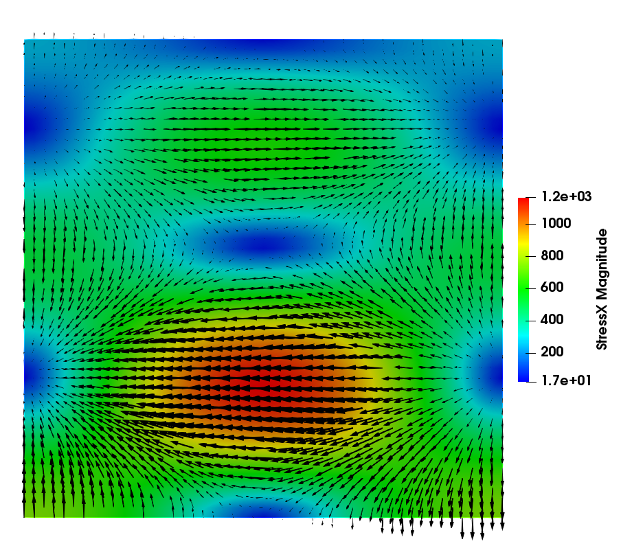
(a) $x$-component of stress

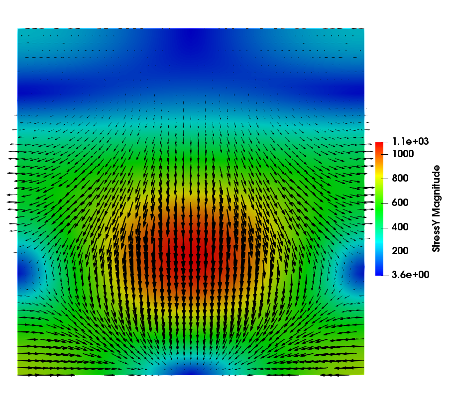
(b) $y$-component of stress

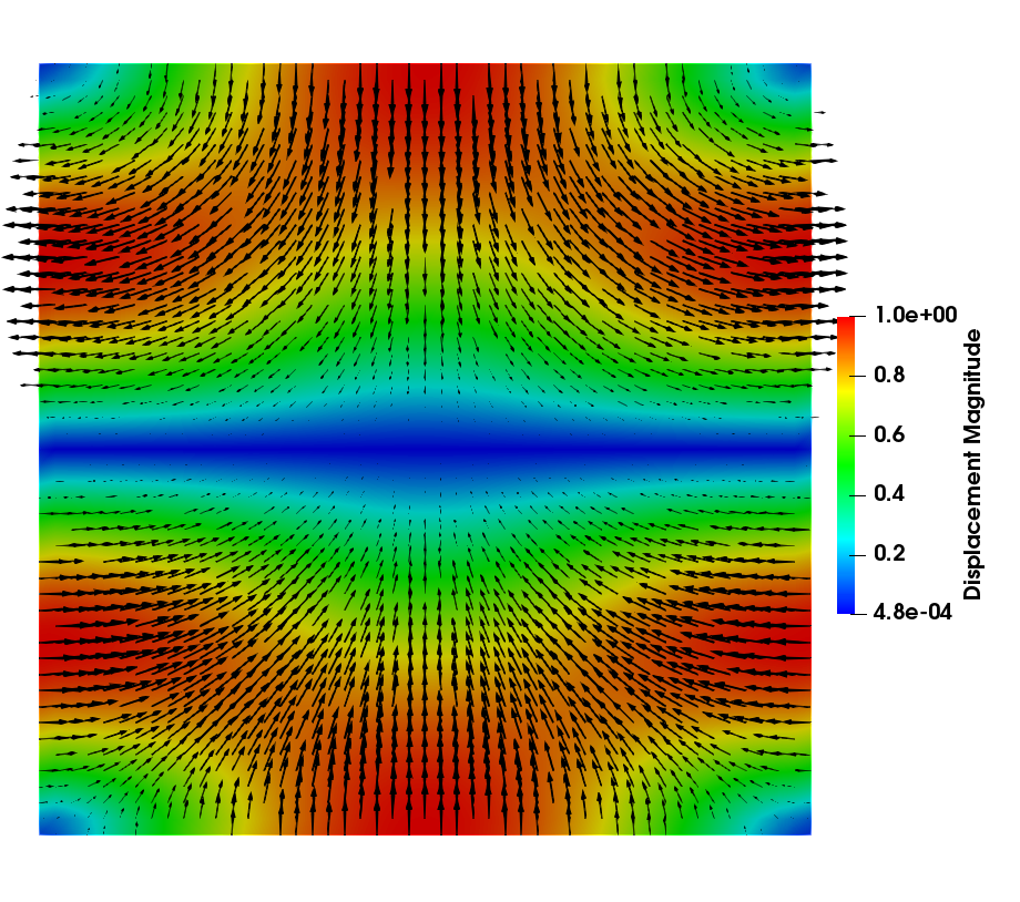
(c) Displacement

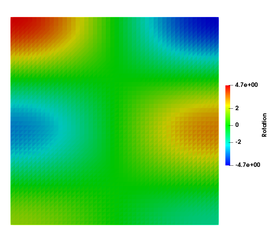
(d) Rotation

Figure 5: Computed solution for Example 1, $h=1/32$

MSMFE-0
	$\|\sigma-\sigma_{h}\|$		$\|\operatorname{div}(\sigma-\sigma_{h})\|$		$\|u-u_{h}\|$		$\|\mathcal{R}^{u}_{h}u-u_{h}\|$		$\|p-p_{h}\|$
$h$	error	rate	error	rate	error	rate	error	rate	error	rate
1/2	8.01E-01	–	8.98E-01	–	8.37E-01	–	8.24E-01	–	1.02E+00	–
1/4	3.58E-01	1.17	4.26E-01	1.09	3.50E-01	1.27	1.82E-01	2.34	5.03E-01	1.02
1/8	1.53E-01	1.23	1.99E-01	1.10	1.73E-01	1.02	4.70E-02	1.96	3.13E-01	0.69
1/16	7.03E-02	1.12	9.84E-02	1.02	8.67E-02	1.00	1.20E-02	1.97	1.71E-01	0.87
1/32	3.42E-02	1.04	5.00E-02	0.98	4.35E-02	0.99	3.03E-03	1.99	8.78E-02	0.96
1/64	1.70E-02	1.01	2.60E-02	0.95	2.18E-02	1.00	7.59E-04	2.00	4.42E-02	0.99
MSMFE-1
	$\|\sigma-\sigma_{h}\|$		$\|\operatorname{div}(\sigma-\sigma_{h})\|$		$\|u-u_{h}\|$		$\|\mathcal{R}^{u}_{h}u-u_{h}\|$		$\|p-p_{h}\|$
$h$	error	rate	error	rate	error	rate	error	rate	error	rate
1/2	7.96E-01	–	9.01E-01	–	8.60E-01	–	8.47E-01	–	9.95E-01	–
1/4	3.67E-01	1.13	4.26E-01	1.09	3.55E-01	1.29	1.95E-01	2.28	4.55E-01	1.12
1/8	1.56E-01	1.23	1.93E-01	1.14	1.76E-01	1.01	5.67E-02	1.78	1.68E-01	1.44
1/16	7.11E-02	1.14	9.34E-02	1.05	8.75E-02	1.01	1.55E-02	1.87	5.37E-02	1.65
1/32	3.43E-02	1.05	4.66E-02	1.00	4.37E-02	1.00	4.01E-03	1.95	1.66E-02	1.70
1/64	1.70E-02	1.02	2.37E-02	0.98	2.18E-02	1.00	1.02E-03	1.98	5.26E-03	1.66

Table 1: Relative errors and convergence rates for Example 1, triangles.

The second test case illustrates the performance of the methods in 3D. We consider the unit cube with homogeneous Dirichlet boundary conditions, analytical solution given by

$$u=\begin{pmatrix}0\\ -(e^{x}-1)(y-\cos(\frac{\pi}{12})(y-\frac{1}{2})+\sin(\frac{\pi}{12})(z-\frac{1}{2})-\frac{1}{2})\\ -(e^{x}-1)(z-\sin(\frac{\pi}{12})(y-\frac{1}{2})-\cos(\frac{\pi}{12})(z-\frac{1}{2})-\frac{1}{2})\end{pmatrix},$$ (6.4)

and Lamé coefficients $\lambda=\mu=100$. The computed solution is shown in Figure 6. In Table 2 we show errors and convergence rates for both methods on a sequence of mesh refinements. Again we observe that the numerical results verify the theoretical convergence rates.

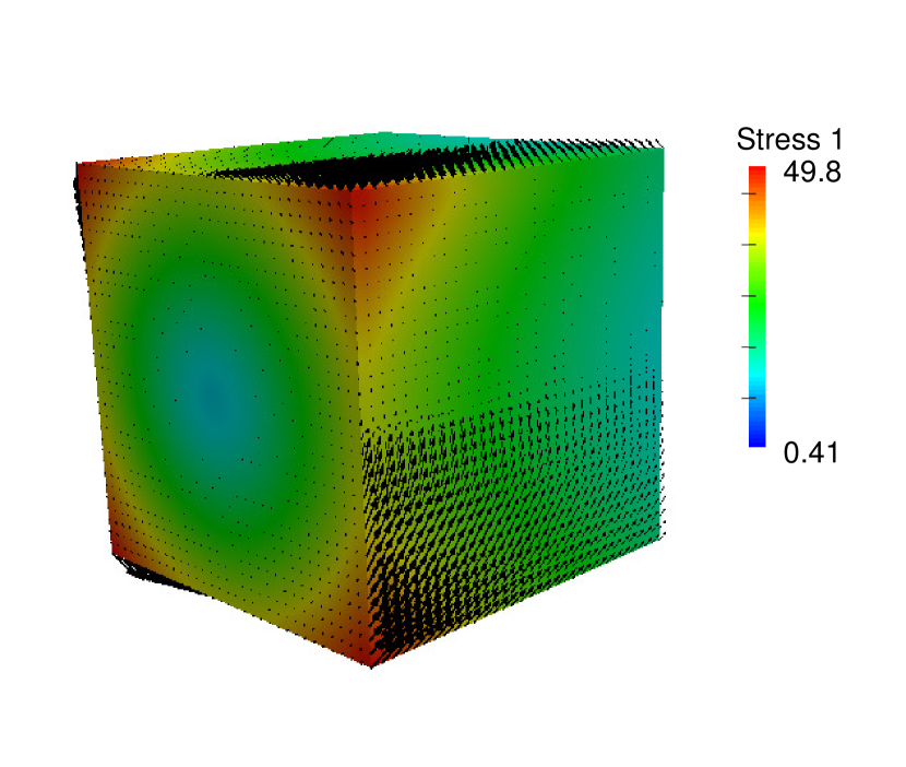
(a) $x$-stress

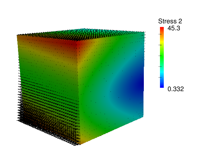
(b) $y$-stress

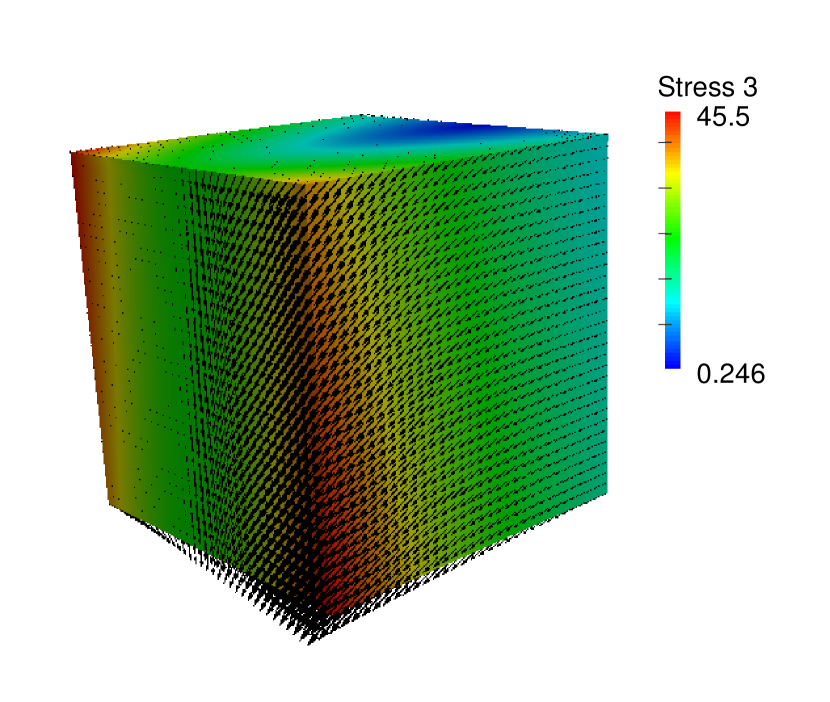
(c) $z$-stress

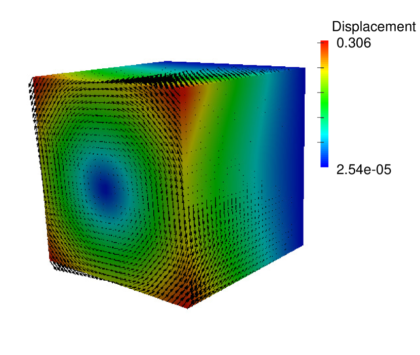
(d) Displacement

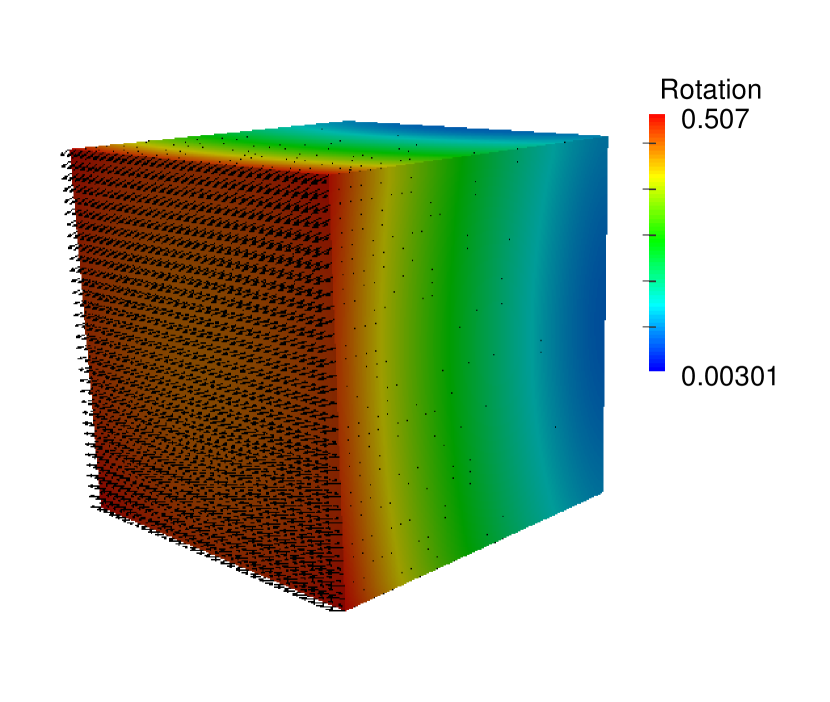
(e) Rotation

Figure 6: Computed solution for Example 2, $h=1/32$

MSMFE-0
	$\|\sigma-\sigma_{h}\|$		$\|\operatorname{div}(\sigma-\sigma_{h})\|$		$\|u-u_{h}\|$		$\|\mathcal{R}^{u}_{h}u-u_{h}\|$		$\|p-p_{h}\|$
$h$	error	rate	error	rate	error	rate	error	rate	error	rate
1/2	4.46E-01	–	2.45E-01	–	4.15E-01	–	1.32E-01	–	2.41E-01	–
1/4	1.96E-01	1.19	1.21E-01	1.02	2.06E-01	1.01	3.11E-02	1.98	1.20E-01	1.00
1/8	9.08E-02	1.11	6.02E-02	1.01	1.03E-01	1.00	7.72E-03	1.98	6.01E-02	1.00
1/16	4.40E-02	1.05	3.01E-02	1.00	5.14E-02	1.00	1.94E-03	1.99	2.99E-02	1.00
1/32	2.17E-02	1.02	1.51E-02	1.00	2.57E-02	1.00	4.85E-04	2.00	1.49E-02	1.00
MSMFE-1
	$\|\sigma-\sigma_{h}\|$		$\|\operatorname{div}(\sigma-\sigma_{h})\|$		$\|u-u_{h}\|$		$\|\mathcal{R}^{u}_{h}u-u_{h}\|$		$\|p-p_{h}\|$
$h$	error	rate	error	rate	error	rate	error	rate	error	rate
1/2	5.40E-01	–	2.45E-01	–	4.20E-01	–	1.55E-01	–	2.38E-01	–
1/4	2.42E-01	1.16	1.21E-01	1.02	2.07E-01	1.02	4.04E-02	1.83	1.00E-01	1.24
1/8	1.09E-01	1.15	6.02E-02	1.01	1.03E-01	1.01	1.07E-02	1.89	3.93E-02	1.35
1/16	5.05E-02	1.12	3.01E-02	1.00	5.14E-02	1.00	2.81E-03	1.93	1.47E-02	1.42
1/32	2.39E-02	1.08	1.51E-02	1.00	2.57E-02	1.00	7.20E-04	1.96	5.38E-03	1.45

Table 2: Relative errors and convergence rates for Example 2, tetrahedra.

Our third example, taken from [41], demonstrates the performance of the MSMFE methods for discontinuous materials. We consider a $3\times 3$ partitioning of the unit square and introduce heterogeneity in the center block through

$$\chi(x,y)=\begin{cases}1\mbox{ if }\min(x,y)>\frac{1}{3}\mbox{ and }\max(x,y)<\frac{2}{3},\\ 0\mbox{ otherwise.}\end{cases}$$

We set $\kappa=10^{6}$ to characterize the jump in the Lamé coefficients and take $\lambda=\mu=(1-\chi)+\kappa\chi$. We choose a continuous displacement solution as

$$u=\frac{1}{(1-\chi)+\kappa\chi}\begin{pmatrix}\sin(3\pi x)\sin(3\pi y)\\ \sin(3\pi x)\sin(3\pi y)\end{pmatrix},$$

so that the stress is also continuous and independent of $\kappa$. The body forces are recovered from the above solution using the governing equations. We note that the rotation $\gamma=\operatorname{Skew}(\nabla u)$ is discontinuous. The MSMFE-0 method, which has discontinuous displacements and rotations, handles properly the discontinuity in these variables and exhibits first order convergence in all variables, as as well as displacement superconvergence, see the top part of Table 3. The MSMFE-1 method uses continuous rotations and does not resolve the rotation discontinuity, which results in a reduced convergence rate for the rotation, as well as the stress. Instead, we can use the modified MSMFE-1 method (4.4)–(4.6) based on the scaled rotation $\tilde{\gamma}=A^{-1}\gamma$, which in this case is continuous. In terms of the implemented method (6.1)–(6.3) with the reduced rotation $p_{h}=\Xi^{-1}(\gamma_{h})$, noting that $\tilde{p}=\Xi^{-1}(\tilde{\gamma})$, the third term in (6.1) becomes $(\tilde{p}_{h},\operatorname{as\,}(A\tau))_{Q}$ and the term in (6.3) becomes $(\operatorname{as\,}(A\sigma_{h}),w)_{Q}$. The computed solution with the modified MSMFE-1 method, including the scaled rotation $\tilde{p}_{h}$, is shown in Figure 7. The bottom part of Table 3 indicates that the method exhibits the same order of convergence for all variables as for smooth problems.

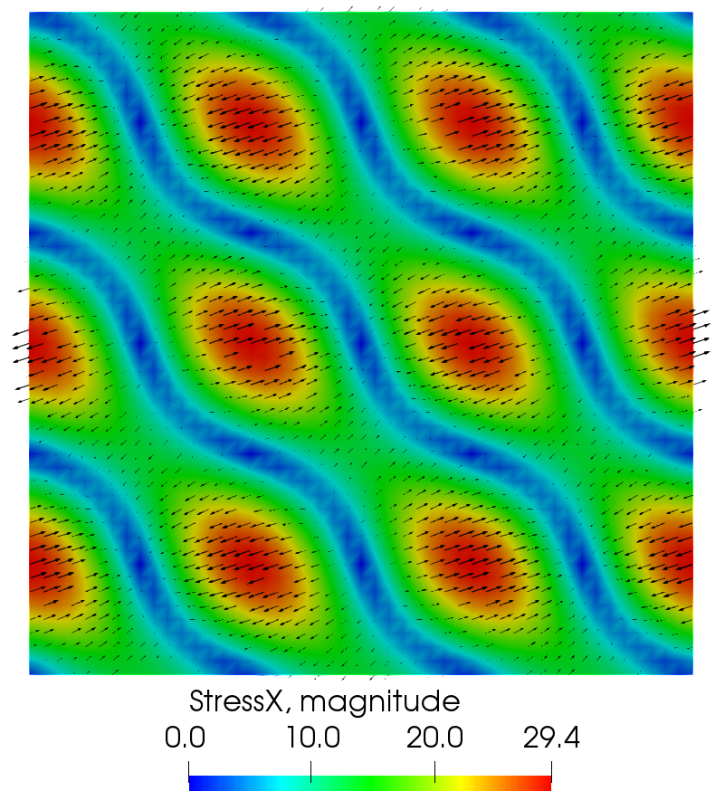
(a) $x$-stress

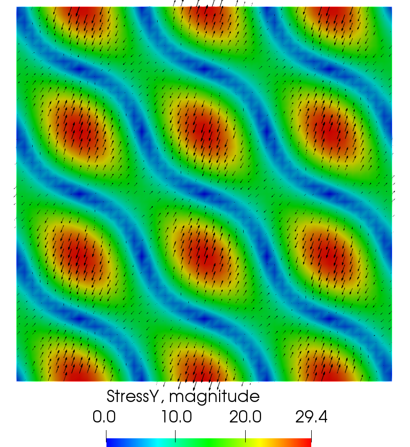
(b) $y$-stress

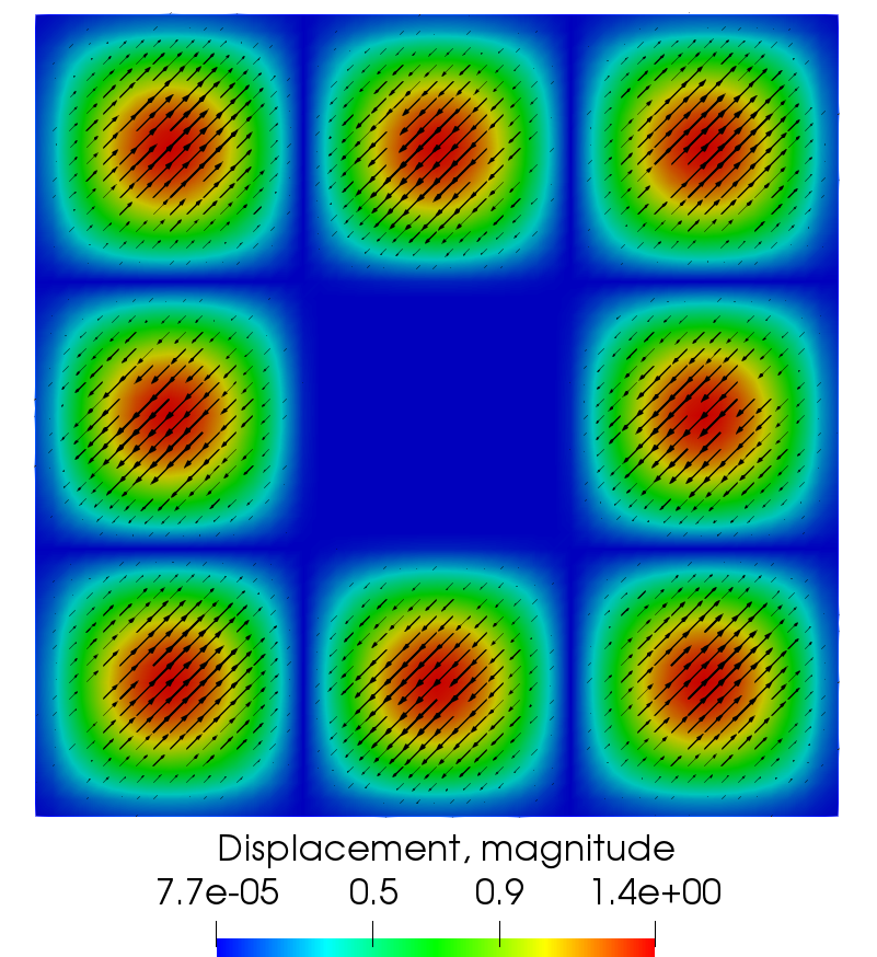
(c) Displacement

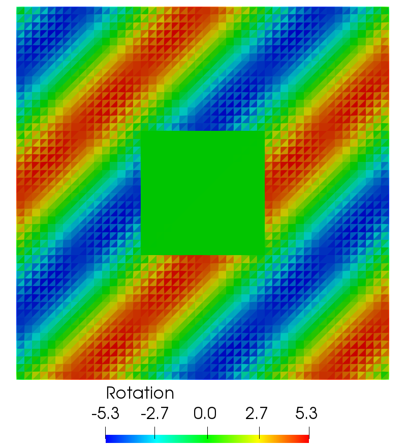
(d) Rotation

(e) Scaled rotation

Figure 7: Computed solution for Example 3, $h=1/48$

MSMFE-0
	$\|\sigma-\sigma_{h}\|$		$\|\operatorname{div}(\sigma-\sigma_{h})\|$		$\|u-u_{h}\|$		$\|\mathcal{R}^{u}_{h}u-u_{h}\|$		$\|p-p_{h}\|$
$h$	error	rate	error	rate	error	rate	error	rate	error	rate
1/3	1.27E+00	-	1.20E+00	-	1.61E+00	-	1.49E+00	-	1.46E+00	-
1/6	6.97E-01	0.87	7.28E-01	0.73	5.87E-01	1.45	4.55E-01	1.71	6.50E-01	1.17
1/12	2.68E-01	1.38	3.33E-01	1.13	2.73E-01	1.10	1.19E-01	1.93	4.70E-01	0.47
1/24	1.05E-01	1.35	1.58E-01	1.07	1.33E-01	1.04	3.08E-02	1.95	2.76E-01	0.77
1/48	4.72E-02	1.16	7.79E-02	1.02	6.57E-02	1.01	7.79E-03	1.98	1.45E-01	0.93
1/96	2.28E-02	1.05	3.88E-02	1.01	3.28E-02	1.00	1.96E-03	1.99	7.34E-02	0.98
MSMFE-1 with scaled rotation
	$\|\sigma-\sigma_{h}\|$		$\|\operatorname{div}(\sigma-\sigma_{h})\|$		$\|u-u_{h}\|$		$\|\mathcal{R}^{u}_{h}u-u_{h}\|$		$\|\tilde{p}-\tilde{p}_{h}\|$
$h$	error	rate	error	rate	error	rate	error	rate	error	rate
1/3	1.26E+00	-	1.20E+00	-	1.73E+00	-	1.59E+00	-	1.20E+00	-
1/6	6.82E-01	0.88	7.28E-01	0.73	5.74E-01	1.59	4.28E-01	1.89	5.46E-01	1.14
1/12	2.60E-01	1.39	3.33E-01	1.13	2.72E-01	1.08	1.17E-01	1.87	2.10E-01	1.38
1/24	1.03E-01	1.34	1.58E-01	1.07	1.33E-01	1.04	3.08E-02	1.92	6.68E-02	1.66
1/48	4.65E-02	1.14	7.79E-02	1.02	6.57E-02	1.01	7.90E-03	1.96	2.11E-02	1.66
1/96	2.26E-02	1.04	3.88E-02	1.01	3.28E-02	1.00	2.01E-03	1.98	6.95E-03	1.60

Table 3: Relative errors and convergence rates for Example 3, triangles.

Our final example, similar to the one in [33], is to study the locking-free property of the MSMFE method. We consider the MSMFE-1 method on the unit square domain with the following boundary conditions: $u=0$ at $y=0$, $\sigma\,n=0$ at $x=0\mbox{ and }x=1$, and $(\sigma\,n)\cdot n=0$, $(\sigma\,n)\cdot t=1$ at $y=1$, where $t$ denotes the unit tangential vector to the side. We recall that the Lamé coefficients are determined from the Young’s modulus $E$ and the Poisson’s ratio $\nu$ via the well-known relationships

$$\lambda=\frac{E\nu}{(1+\nu)(1-2\nu)},\quad\mu=\frac{E}{2(1+\nu)}.$$

We fix the Young’s modulus $E=10^{5}$ and vary the Poisson’s ratio $\nu=0.5-k$, $k=1e-l$, for $l=\{1,2,5,9\}$. Locking would result in the displacement solution going to zero as $\nu$ approaches $0.5$. In Figure 8 (left) we see that such behavior is not present, confirming the robustness of the method for almost incompressible materials. In addition, a plot of the displacement magnitude along the top side of the square ($y=1$) for various choices of $k$ is shown in the Figure 8 (right). One can see that there is little change in the displacement solution when $\nu\to 0.5$.

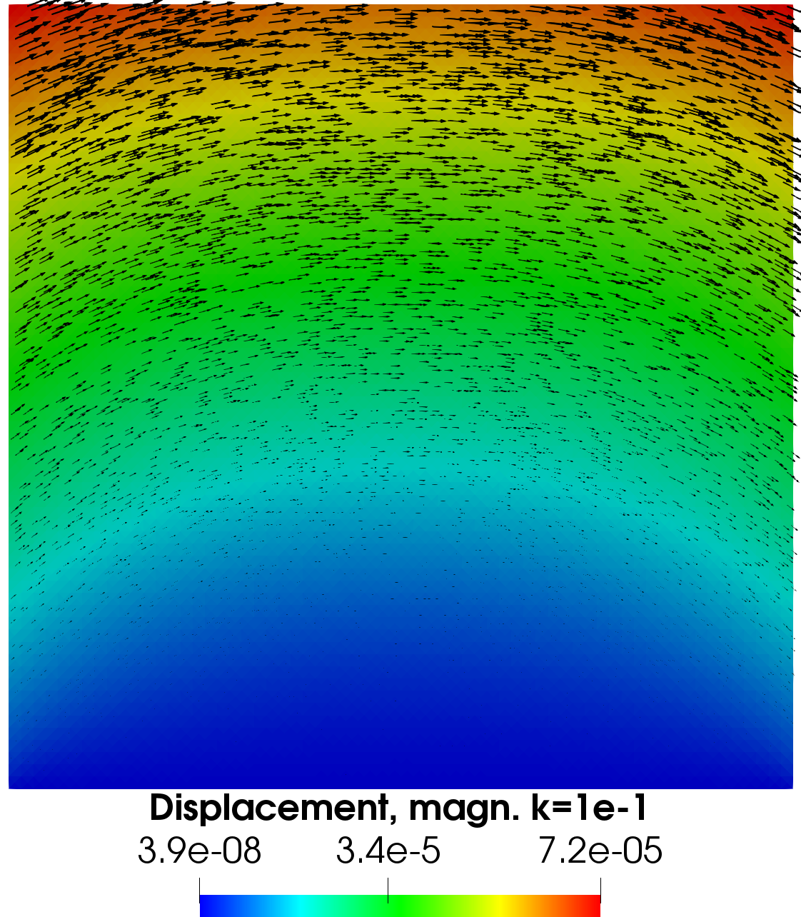
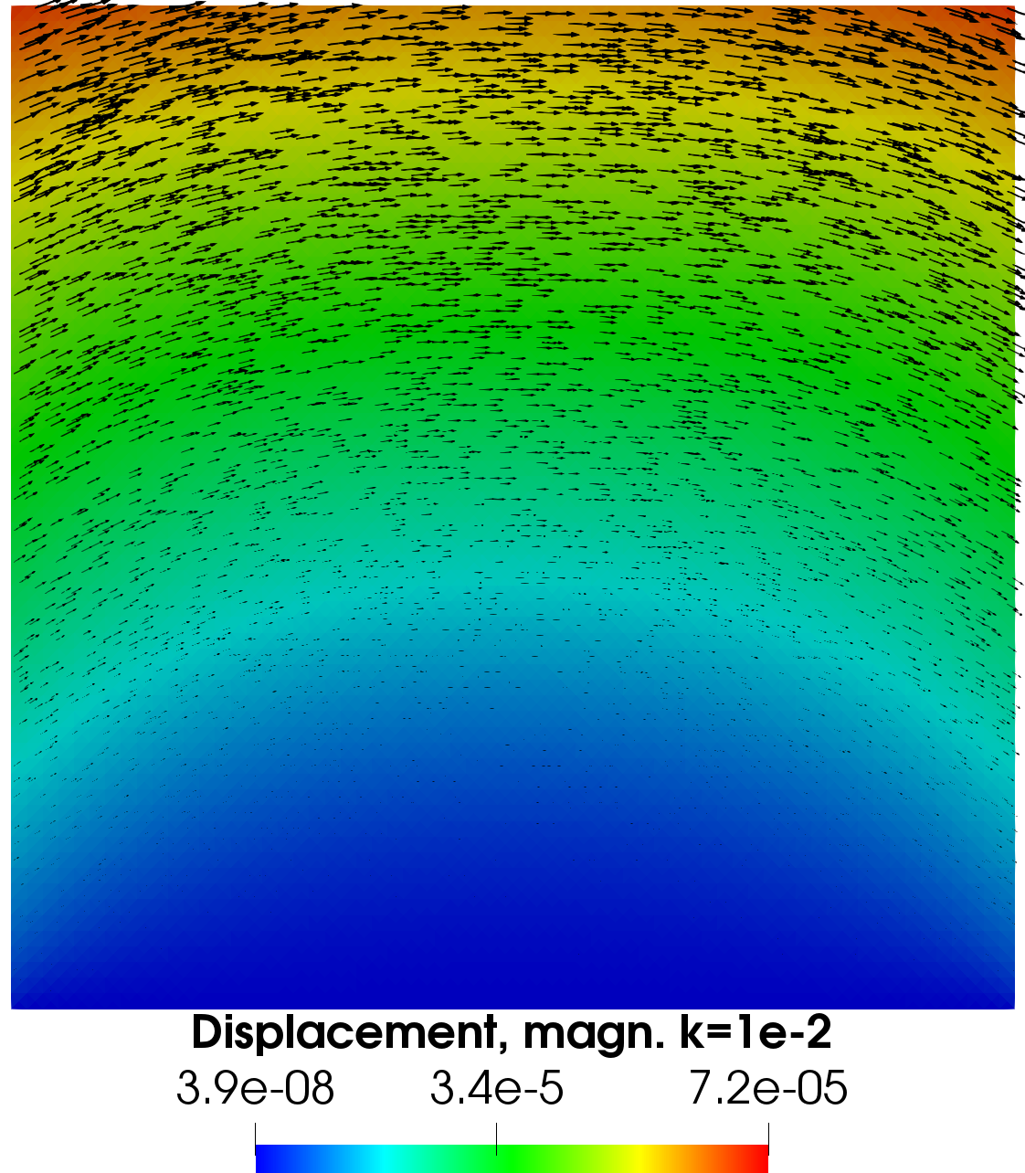
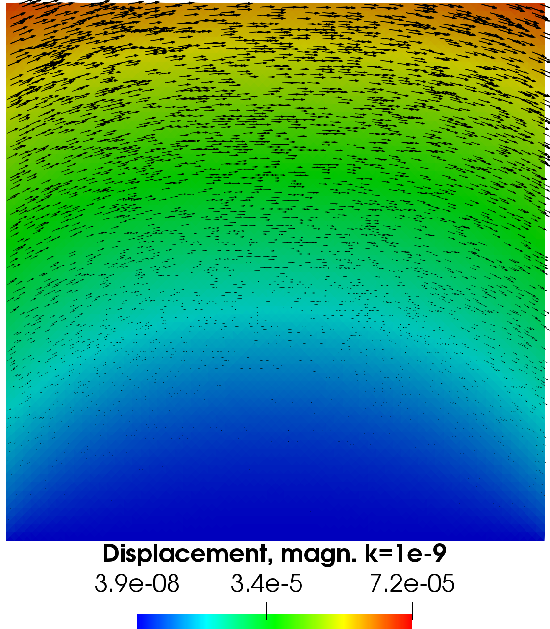
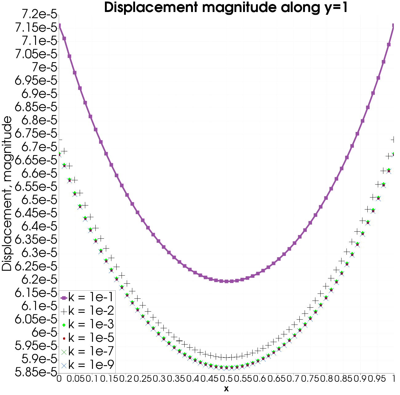
Figure 8: Computed displacement solutions for Example 4, $h=1/32$.

7 Conclusion

We presented two $\mathcal{BDM}_{1}$-based MFE methods with quadrature for elasticity with weak stress symmetry on simplicial grids. The MSMFE-0 method reduces to a cell-centered scheme for displacements and rotations, while the MSMFE-1 method reduces to a cell-centered scheme for displacements only. To prove stability of the MSMFE-1 method, we established a discrete inf-sup condition with quadrature for the Stokes problem. We showed that the resulting algebraic system for each of the methods is symmetric and positive definite. We proved first order convergence for all variables in their natural norms, as well as second order convergence for the displacements at the cell centers. The methods can also be developed on quadrilateral grids, which is the subject of a forthcoming paper.

References

- [1] I. Aavatsmark. An introduction to multipoint flux approximations for quadrilateral grids. Comput. Geosci., 6(3-4):405–432, 2002. Locally conservative numerical methods for flow in porous media.
- [2] I. Aavatsmark, T. Barkve, O. Bøe, and T. Mannseth. Discretization on unstructured grids for inhomogeneous, anisotropic media. II. Discussion and numerical results. SIAM J. Sci. Comput., 19(5):1717–1736, 1998.
- [3] L. Agélas, C. Guichard, and R. Masson. Convergence of finite volume MPFA O type schemes for heterogeneous anisotropic diffusion problems on general meshes. International Journal on Finite Volumes, pages volume–7, 2010.
- [4] T. Arbogast, C. N. Dawson, P. T. Keenan, M. F. Wheeler, and I. Yotov. Enhanced cell-centered finite differences for elliptic equations on general geometry. SIAM J. Sci. Comp., 19(2):404–425, 1998.
- [5] T. Arbogast, M. F. Wheeler, and I. Yotov. Mixed finite elements for elliptic problems with tensor coefficients as cell-centered finite differences. SIAM J. Numer. Anal., 34(2):828–852, 1997.
- [6] D. N. Arnold and G. Awanou. Rectangular mixed finite elements for elasticity. Math. Models Methods Appl. Sci., 15(9):1417–1429, 2005.
- [7] D. N. Arnold, G. Awanou, and W. Qiu. Mixed finite elements for elasticity on quadrilateral meshes. Adv. Comput. Math., 41(3):553–572, 2015.
- [8] D. N. Arnold, G. Awanou, and R. Winther. Nonconforming tetrahedral mixed finite elements for elasticity. Math. Models Methods Appl. Sci., 24(4):783–796, 2014.
- [9] D. N. Arnold, F. Brezzi, and J. Douglas, Jr. PEERS: a new mixed finite element for plane elasticity. Japan J. Appl. Math., 1(2):347–367, 1984.
- [10] D. N. Arnold, R. S. Falk, and R. Winther. Mixed finite element methods for linear elasticity with weakly imposed symmetry. Math. Comp., 76(260):1699–1723, 2007.
- [11] D. N. Arnold and R. Winther. Mixed finite elements for elasticity. Numer. Math., 92(3):401–419, 2002.
- [12] D. N. Arnold and R. Winther. Nonconforming mixed elements for elasticity. Math. Models Methods Appl. Sci., 13(3):295–307, 2003. Dedicated to Jim Douglas, Jr. on the occasion of his 75th birthday.
- [13] G. Awanou. Rectangular mixed elements for elasticity with weakly imposed symmetry condition. Adv. Comput. Math., 38(2):351–367, 2013.
- [14] L. Beirão da Veiga, F. Brezzi, and L. D. Marini. Virtual elements for linear elasticity problems. SIAM J. Numer. Anal., 51(2):794–812, 2013.
- [15] D. Boffi, F. Brezzi, L. F. Demkowicz, R. G. Durán, R. S. Falk, and M. Fortin. Mixed finite elements, compatibility conditions, and applications, volume 1939 of Lecture Notes in Mathematics. Springer-Verlag, Berlin; Fondazione C.I.M.E., Florence, 2008. Lectures given at the C.I.M.E. Summer School held in Cetraro, June 26–July 1, 2006, Edited by Boffi and Lucia Gastaldi.
- [16] D. Boffi, F. Brezzi, and M. Fortin. Reduced symmetry elements in linear elasticity. Commun. Pure Appl. Anal., 8(1):95–121, 2009.
- [17] S. C. Brenner and L.-Y. Sung. Linear finite element methods for planar linear elasticity. Math. Comp., 59(200):321–338, 1992.
- [18] F. Brezzi, J. Douglas, Jr., and L. D. Marini. Two families of mixed finite elements for second order elliptic problems. Numer. Math., 47(2):217–235, 1985.
- [19] F. Brezzi and M. Fortin. Mixed and hybrid finite element methods, volume 15 of Springer Series in Computational Mathematics. Springer-Verlag, New York, 1991.
- [20] F. Brezzi, M. Fortin, and L. D. Marini. Error analysis of piecewise constant pressure approximations of Darcy’s law. Comput. Methods Appl. Mech. Eng., 195:1547–1559, 2006.
- [21] P. G. Ciarlet. The finite element method for elliptic problems. SIAM, 2002.
- [22] B. Cockburn, J. Gopalakrishnan, and J. Guzmán. A new elasticity element made for enforcing weak stress symmetry. Math. Comp., 79(271):1331–1349, 2010.
- [23] B. Cockburn and K. Shi. Superconvergent HDG methods for linear elasticity with weakly symmetric stresses. IMA J. Numer. Anal., 33(3):747–770, 2013.
- [24] D. A. Di Pietro and A. Ern. A hybrid high-order locking-free method for linear elasticity on general meshes. Comput. Methods Appl. Mech. Engrg., 283:1–21, 2015.
- [25] D. A. Di Pietro, R. Eymard, S. Lemaire, and R. Masson. Hybrid finite volume discretization of linear elasticity models on general meshes. In Finite volumes for complex applications. VI. Problems & perspectives. Volume 1, 2, volume 4 of Springer Proc. Math., pages 331–339. Springer, Heidelberg, 2011.
- [26] D. A. Di Pietro and S. Lemaire. An extension of the Crouzeix-Raviart space to general meshes with application to quasi-incompressible linear elasticity and Stokes flow. Math. Comp., 84(291):1–31, 2015.
- [27] M. G. Edwards. Unstructured, control-volume distributed, full-tensor finite-volume schemes with flow based grids. Comput. Geosci., 6(3-4):433–452, 2002. Locally conservative numerical methods for flow in porous media.
- [28] M. G. Edwards and C. F. Rogers. Finite volume discretization with imposed flux continuity for the general tensor pressure equation. Comput. Geosci., 2(4):259–290 (1999), 1998.
- [29] G. P. Galdi. An introduction to the mathematical theory of the Navier-Stokes equations. Vol. I. Springer-Verlag, New York, 1994. Linearized steady problems.
- [30] J. Gopalakrishnan and J. Guzmán. Symmetric nonconforming mixed finite elements for linear elasticity. SIAM J. Numer. Anal., 49(4):1504–1520, 2011.
- [31] J. Gopalakrishnan and J. Guzmán. A second elasticity element using the matrix bubble. IMA J. Numer. Anal., 32(1):352–372, 2012.
- [32] P. Grisvard. Elliptic problems in nonsmooth domains, volume 24 of Monographs and Studies in Mathematics. Pitman (Advanced Publishing Program), Boston, MA, 1985.
- [33] P. Hansbo and M. G. Larson. Discontinuous Galerkin and the Crouzeix-Raviart element: application to elasticity. M2AN Math. Model. Numer. Anal., 37(1):63–72, 2003.
- [34] R. A. Horn and C. R. Johnson. Matrix analysis. Cambridge University Press, Cambridge, second edition, 2013.
- [35] R. Ingram, M. F. Wheeler, and I. Yotov. A multipoint flux mixed finite element method on hexahedra. SIAM J. Numer. Anal., 48(4):1281–1312, 2010.
- [36] E. Keilegavlen and J. M. Nordbotten. Finite volume methods for elasticity with weak symmetry. Int. J. Numer. Meth. Engng., 112(8):939–962, 2017.
- [37] R. A. Klausen and R. Winther. Robust convergence of multi point flux approximation on rough grids. Numer. Math., 104(3):317–337, 2006.
- [38] J. J. Lee. Towards a unified analysis of mixed methods for elasticity with weakly symmetric stress. Adv. Comput. Math., 42(2):361–376, 2016.
- [39] J.-L. Lions and E. Magenes. Non-homogeneous boundary value problems and applications. Vol. II. Springer-Verlag, New York-Heidelberg, 1972. Translated from the French by P. Kenneth, Die Grundlehren der mathematischen Wissenschaften, Band 182.
- [40] A. Logg, K.-A. Mardal, G. N. Wells, et al. Automated Solution of Differential Equations by the Finite Element Method. Springer, 2012.
- [41] J. M. Nordbotten. Cell-centered finite volume discretizations for deformable porous media. Internat. J. Numer. Methods Engrg., 100(6):399–418, 2014.
- [42] J. M. Nordbotten. Convergence of a cell-centered finite volume discretization for linear elasticity. SIAM J. Numer. Anal., 53(6):2605–2625, 2015.
- [43] W. Qiu, J. Shen, and K. Shi. An HDG method for linear elasticity with strong symmetric stresses. Math. Comp., 87(309):69–93, 2018.
- [44] B. Rivière and M. F. Wheeler. Optimal error estimates for discontinuous Galerkin methods applied to linear elasticity problems. Comput. Math. Appl, 46:141–163, 2000.
- [45] T. F. Russell and M. F. Wheeler. Finite element and finite difference methods for continuous flows in porous media. The mathematics of reservoir simulation, 1:35–106, 1983.
- [46] R. Stenberg. Analysis of mixed finite elements methods for the Stokes problem: a unified approach. Math. Comp., 42(165):9–23, 1984.
- [47] R. Stenberg. A family of mixed finite elements for the elasticity problem. Numer. Math., 53(5):513–538, 1988.
- [48] C. Wang, J. Wang, R. Wang, and R. Zhang. A locking-free weak Galerkin finite element method for elasticity problems in the primal formulation. J. Comput. Appl. Math., 307:346–366, 2016.
- [49] M. F. Wheeler, G. Xue, and I. Yotov. A multipoint flux mixed finite element method on distorted quadrilaterals and hexahedra. Numer. Math., 121(1):165–204, 2012.
- [50] M. F. Wheeler and I. Yotov. A multipoint flux mixed finite element method. SIAM J. Numer. Anal., 44(5):2082–2106, 2006.