Machine-learning inference of fluid variables from data using reservoir computing

Abstract

We infer both microscopic and macroscopic behaviors of a three-dimensional chaotic fluid flow using reservoir computing. In our procedure of the inference, we assume no prior knowledge of a physical process of a fluid flow except that its behavior is complex but deterministic. We present two ways of inference of the complex behavior; the first called partial-inference requires continued knowledge of partial time-series data during the inference as well as past time-series data, while the second called full-inference requires only past time-series data as training data. For the first case, we are able to infer long-time motion of microscopic fluid variables. For the second case, we show that the reservoir dynamics constructed from only past data of energy functions can infer the future behavior of energy functions and reproduce the energy spectrum. It is also shown that we can infer a time-series data from only one measurement by using the delay coordinates. These implies that the obtained two reservoir systems constructed without the knowledge of microscopic data are equivalent to the dynamical systems describing macroscopic behavior of energy functions.

I I. Introduction

Machine-learning has progressed significantly over the last decade in various areas of physical sciences Snyder et al. (2012); Gabbard et al. (2018); Mills and Tamblyn (2018) after some theoretical works in the area of neural networks (See Hornik et al. (1989); Cybenko (1989) for examples.)
In fluid dynamics area Ling et al. (2016) presents a method of using deep neural networks to learn a model for the Reynolds stress anisotropy tensor from high-fidelity simulation data (see also Kutz (2017)). Gamahara and Hattori (2017) uses an artificial neural network to find a new subgrid model of the subgrid-scale stress in large-eddy simulation. By using “Long Short-Term Memory (LSTM)” Hochreiter and Schmidhuber (1997), Wan et al. (2018) studies a data-assisted reduced-order modeling of extreme events in various dynamics including the Kolomogorov flow of the two-dimensional incompressible Navier–Stokes equation. See also Vlachas et al. (2018) for the result on the barotropic climate model.
It is recently reported that reservoir computing, brain-inspired machine-learning framework that employs a data-driven dynamical system, is effective in the inference of a future such as time-series, frequency spectra and the Lyapunov spectra Verstraeten et al. (2007); Inubushi and Yoshimura (2017); Lu et al. (2017); Pathak et al. (2017); Ibáñez-Soria et al. (2018); Pathak et al. (2018); Antonik et al. (2018). Pathak et al. (2017) exemplifies using the Lorenz system and the Kuramoto-Sivashinsky system that the model obtained by reservoir computing can generate an arbitrarily long time-series whose Lyapunov exponents approximate those of the input signal.
A reservoir is a recurrent neural network whose internal parameters are not adjusted to fit the data in the training process. What is done is to train the reservoir by feeding it an input time-series and fitting a linear function of the reservoir state variables to a desired output time-series. Due to this approach of reservoir computing we can save a great amount of computational costs, which enables us to deal with a complex deterministic behavior. The framework was proposed as Echo-State Networks Jaeger (2001); Jaeger and Haas (2004) and Liquid-State Machines Maass et al. (2002).
It is known that an inference of a fluid flow is difficult but important in both physical and industrial aspects. In this paper, we infer variables of a chaotic fluid flow by applying the method of reservoir computing without a prior knowledge of physical process.
After introducing the method of reservoir computing in Section II and a fluid flow in Section III, we explain how to apply the method to the inference of fluid variables, and show that inferences of both microscopic and macroscopic behaviors are successful in Sections IV and V, respectively. In Section VI, we exemplify that a time-series inference of high-dimensional dynamics is possible by using delay coordinates, even when the number of measurements is smaller than the Lyapunov dimension of the attractor. Discussions and remarks are given in Section VII.

II II. Reservoir computing

Reservoir computing is recently used in the inference of complex dynamics Lu et al. (2017); Pathak et al. (2017, 2018); Ibáñez-Soria et al. (2018); Lu et al. (2018). The reservoir computing focuses on the determination of a translation matrix from reservoir state variables to variables to be inferred (see eq. (4)). Here we review the outline of the method Jaeger and Haas (2004); Lu et al. (2017). We consider a dynamical system

$$\frac{d\mathbf{\phi}}{dt}=\mathbf{f}(\mathbf{\phi}),$$

together with a pair of $\phi$-dependent, vector valued variables

$$\mathbf{u}=\mathbf{h}_{1}(\mathbf{\phi})\in\mathbb{R}^{M}~{}~{}\text{and}~{}~{}\mathbf{s}=\mathbf{h}_{2}(\mathbf{\phi})\in\mathbb{R}^{P}.$$

We seek a method for using the continued knowledge of $\mathbf{u}$ to determine an estimate of $\mathbf{s}$ as a function of time when direct measurement of $\mathbf{s}$ is not available, which we call the partial-inference. We also consider the full-inference for which we have a knowledge $\mathbf{u}$ only for $t\leq T$. Concerning the algorithm, this is just a variant of the partial-inference Pathak et al. (2017, 2018), and will be explained later.
The dynamics of the reservoir state vector

$$\mathbf{r}\in\mathbb{R}^{N}~{}(N\gg M),$$

is defined by

$$\mathbf{r}(t+\Delta t)=(1-\alpha)\mathbf{r}(t)+\alpha\tanh(\mathbf{A}\mathbf{r}(t)+\mathbf{W}_{\text{in}}\mathbf{u}(t)),$$ (1)

where $\Delta t$ is a relatively short time step. The matrix $\mathbf{A}$ is a weighted adjacency matrix of the reservoir layer, and the $M$-dimensional input $\mathbf{u}(t)$ is fed in to the $N$ reservoir nodes via a linear input weight matrix denoted by $\mathbf{W}_{\text{in}}$. The parameter $\alpha$ ($0<\alpha\leq 1$) in eq. (1) adjusts the nonlinearity of the dynamics of $\mathbf{r}$, and is chosen depending upon the complexity of the dynamics of measurements and the time step $\Delta t$.
Each row of $\mathbf{W}_{\text{in}}$ has one nonzero element, chosen from a uniform distribution on $[-\sigma,\sigma]$. The matrix $\mathbf{A}$ is chosen from a sparse random matrix in which the fraction of nonzero matrix elements is $(D_{1}+D_{2})/N$, so that the average degree of a reservoir node is $D_{1}+D_{2}$. The $D_{1}$ non-zero components are chosen from a uniform distribution on $[-1,1]$, and $D_{2}$ from that on $[-\gamma,\gamma]$ for $\gamma~{}(\ll 1)$, where $D_{2}$ non-zero components are introduced to reflect weak couplings among components of $\mathbf{r}$. Then we uniformly rescale all the elements of $\mathbf{A}$ so that the largest value of the magnitudes of its eigenvalues becomes $\rho$.
The output, which is a $P$-dimensional vector, is taken to be a linear function of the reservoir state $\mathbf{r}$:

$$\hat{\mathbf{s}}(t)=\mathbf{W}_{out}\mathbf{r}(t)+\mathbf{c}.$$ (2)

The reservoir state $\mathbf{r}$ evolves following eq. (1) with input $\mathbf{u}(t)$, starting from random initial state $\mathbf{r}(-\tau)$ whose elements are chosen from $(0,1]$ in order not to diverge, where $\tau/\Delta t~{}(\gg 1)$ is the transient time. We obtain $L=T/\Delta t$ steps of reservoir states $\{\mathbf{r}(l\Delta t)\}_{l=1}^{L}$ by eq. (1). Moreover, we record the actual measurements of the state variables $\{\mathbf{s}(l\Delta t)\}_{l=1}^{L}$.
We train the network by determining $\mathbf{W}_{\text{out}}$ and $\mathbf{c}$ so that the reservoir output approximates the measurement for $0<t\leq T$ (training phase), which is the main part of this computation. We do this by minimizing the following quadratic form with respect to $\mathbf{W}_{\text{out}}$ and $\mathbf{c}$:

$$\sum^{L}_{l=1}\|(\mathbf{W}_{\text{out}}\mathbf{r}(l\Delta t)+\mathbf{c})-\mathbf{s}(l\Delta t)\|^{2}+\beta[Tr(\mathbf{W}_{\text{out}}\mathbf{W}^{T}_{\text{out}})],$$ (3)

where $\|\mathbf{q}\|^{2}=\mathbf{q}^{T}\mathbf{q}$ for a vector $\mathbf{q}$, and the second term is a regularization term introduced to avoid overfitting $\mathbf{W}_{\text{out}}$ for $\beta\geq 0$. When the training is successful, $\hat{\mathbf{s}}(t)$ should approximate the desired unmeasured quantity $\mathbf{s}(t)$ for $t>T$ (inference phase). Following eq. (2), we obtain

$$\hat{\mathbf{s}}(t)=\mathbf{W}^{*}_{\text{out}}\mathbf{r}(t)+c^{*},$$ (4)

where $\mathbf{W}^{*}_{\text{out}}$ and $c^{*}$ denote the solutions for the minimizers of the quadratic form (3) (see Lukosevivcius and Jaeger (2009) P.140 for details):

$$\mathbf{W}^{*}_{\text{out}} =\delta\mathbf{S}\delta\mathbf{R}^{T}(\delta\mathbf{R}\delta\mathbf{R}^{T}+\beta\mathbf{I})^{-1},$$

$$c^{*} =-[\mathbf{W}^{*}_{\text{out}}\overline{\mathbf{r}}-\overline{\mathbf{s}}],$$

where $\overline{r}=\sum^{L}_{l=1}\mathbf{r}(l\Delta t)$/L, $\overline{s}=\sum^{L}_{l=1}\mathbf{s}(l\Delta t)/L$, and $\mathbf{I}$ is the $N\times N$ identity matrix, $\delta\mathbf{R}$ (respectively, $\delta\mathbf{S}$) is the matrix whose $l$-th column is $\mathbf{r}(l\Delta t)-\overline{r}$ (respectively, $\mathbf{s}(l\Delta t)-\overline{s}$).

parameter		(a)	(b)	(c)
$\tau$	transient time	1000	2500	2350
$T$	training time	10000	20000	20000
$M$	dimension of measurements	270	9	36
$P$	dimension of inferred variables	2	9	36
$N$	number of reservoir nodes	6400	3200	3200
$D_{1}$	parameter of determining elements of $\mathbf{A}$	60	320	120
$D_{2}$	parameter of determining elements of $\mathbf{A}$	60	0	0
$\gamma$	scale of input weights in $\mathbf{A}$	0.1	0	0
$\rho$	maximal eigenvalue of $\mathbf{A}$	1.0	0.5	0.5
$\sigma$	scale of input weights in $\mathbf{W}_{in}$	0.4	0.3	0.5
$\alpha$	nonlinearity degree of reservoir dynamics	0.7	0.3	0.4
$\Delta t$	time step for reservoir dynamics	0.1	0.25	0.5
$\beta$	regularization parameter	0	0.01	0.1

Table 1: Sets of parameters for our reservoir computing. The set (a) is used for the partial-inference of microscopic Fourier variables, whereas the set (b) is for the full-inference of macroscopic variables of energy functions and energy spectrum, and the set (c) is for the full-inference from only one measurement.

In order to consider the effect of all the variables equally, we take the normalized value $\tilde{X}(t)$ for each variable $X(t)$, which will be used throughout the whole procedure of our reservoir computing:

$$\tilde{X}(t)=[X(t)-X_{1}]/X_{2},$$

where $X_{1}$ is the mean value and $X_{2}$ is the variance. When we reconstruct $X(t)$ in the inference phase from $\tilde{X}(t)$, we employ $X_{1}$ and $X_{2}$ obtained in the training phase. Due to the normalization we can avoid adjustments of $\sigma$.

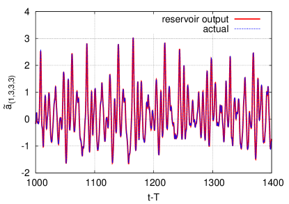
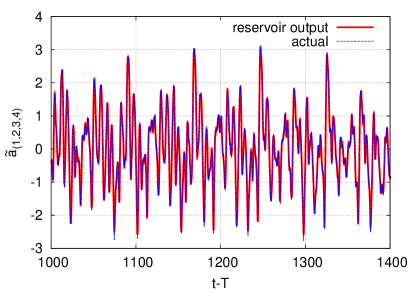
Figure 1: Partial-inference of time-series of microscopic variables in Fourier space of a fluid flow. Fourier variables ${\tilde{a}}_{\eta_{1}=(1,3,3,3)}$ (top) and ${\tilde{a}}_{\eta_{2}=(1,2,3,4)}$ (bottom) are inferred by using measured variables $\tilde{a}_{\eta}$ for $\eta\in S$ as well as the past time-series data for all the measured variables $\tilde{a}_{\eta}$ for $\eta\in S\cup\{\eta_{1},\eta_{2}\}$. We can observe that the inferred time-series almost coincide with the actual ones obtained by the direct numerical simulation of the Navier–Stokes equation even after sufficiently large time has passed since the training phase finished. The inference errors in $l^{1}$-norm averaged over $t-T\in[0,2000]$ are $1.8\%$ and $3.5\%$ for $\tilde{a}_{\eta_{1}}$ and $\tilde{a}_{\eta_{2}}$, respectively.

III III. Fluid flow

In order to generate measurements of the reservoir computing, we employ the direct numerical simulation of the incompressible three-dimensional Navier–Stokes equation under periodic boundary conditions:

$$\begin{cases}\partial_{t}v-\nu\Delta v+(v\cdot\nabla)v+\nabla\pi=f,~{}\nabla\cdot v=0,~{}\mathbb{T}^{3}\times(0,\infty),\\ v\big{|}_{t=0}=v_{0}\quad\text{with $\nabla\cdot v_{0}=0$},~{}~{}~{}~{}~{}~{}~{}~{}~{}~{}~{}~{}~{}~{}~{}~{}~{}~{}~{}~{}\mathbb{T}^{3},\end{cases}$$

where ${\mathbb{T}}=[0,2\pi)$, $\nu>0$ is viscosity parameter, $\pi(x,t)$ is pressure, and $v(x,t)=(v_{1}(x,t),v_{2}(x,t),v_{3}(x,t))$ is velocity. We use the Fourier spectral method Ishioka (1999) with $N_{0}(=9)$ modes in each direction, meaning that the system is approximated by $2(2N_{0}+1)^{3}~{}(=13718)$-dimensional ordinary differential equations (ODEs). The ODEs are integrated by the 4th-order Runge–Kutta method, and the forcing is input into the low-frequency variables at each time step so as to preserve the energy of the low-frequency part. That is, both the real and the imaginary parts of the Fourier coefficient of the vorticity $\omega~{}(=\text{rot}~{}v)$,

$$\mathcal{F}_{[\omega_{\zeta}]}(\kappa,t):=\dfrac{1}{(2\pi)^{3}}\displaystyle\int_{\mathbb{T}^{3}}\omega_{\zeta}(x,t)e^{-i(\kappa\cdot x)}dx,$$

are kept constant for $\zeta=1,2$, $\kappa=(1,0,0),(0,1,0)$. We use an initial condition, which has energy only in the low-frequency variables. See Ishioka (1999) for the details.

IV IV. Partial-inference of microscopic variables: Fourier variables of velocity.

We consider the absolute value of Fourier variables of velocity $\mathcal{F}_{[v_{\zeta}]}(\kappa,t)$ as the representative microscopic variables:

$$a_{\eta}(t)=\left|\mathcal{F}_{[v_{\zeta}]}(\kappa,t)\right|:=\left|\dfrac{1}{(2\pi)^{3}}\int_{\mathbb{T}^{3}}v_{\zeta}(x,t)e^{-i(\kappa\cdot x)}dx\right|,$$ (5)

where $\eta=(\zeta,\kappa)\in S_{0}:=\{(\zeta,\kappa_{1},\kappa_{2},\kappa_{3})\in\mathbb{Z}^{4}|~{}\zeta\in\{1,2,3\},\kappa_{1},\kappa_{2},\kappa_{3}\in[-N_{0},N_{0}]\}$. Since $v$ is real, $a_{(\cdot,\kappa_{1},\kappa_{2},\kappa_{3})}=a_{(\cdot,-\kappa_{1},-\kappa_{2},-\kappa_{3})}$. The reason why we take the absolute value in eq. (5) is to kill the rotational invariance of a complex variable and to make an inference possible. We choose a chaotic parameter $\nu=0.05862$, and set $\mathbf{u}(t)$ as the time-series of $M=270$ Fourier variables $\tilde{a}_{\eta}$, where $\eta\in S:=\{(2,\pm\kappa_{1},\kappa_{2},\kappa_{3})\in\mathbb{Z}^{4}|~{}1\leq\kappa_{1}\leq N_{0},\kappa_{1}\leq\kappa_{2}\leq\kappa_{3}\leq\kappa_{1}+4\}$ and each component is taken $\bmod~{}N_{0}$, that is,

$$\mathbf{u}(t) =(\{\tilde{a}_{\eta}\}_{\eta\in S})^{t}.$$

We also set

$$\mathbf{s}(t) =(\tilde{a}_{(1,3,3,3)},\tilde{a}_{(1,2,3,4)})^{t},$$

where $(1,3,3,3),(1,2,3,4)\notin S$. Under the set of parameters in TABLE 1 (a) we infer the time-series $\mathbf{s}(t)$, which is successful for quite a long time (see Fig. 1).
The choice of variables to be trained is not very significant in this study, because the attractor does not show a homogeneous isotropic turbulence, and it has less symmetries. We can see from the Poincaré section of the microscopic variables that the flow is not isotropic and indeterminacy in inference due to the continuous symmetry does not appear. However, by training variables with different types of behaviors, we can construct a reservoir model in less computational costs with lower dimension $N$ of the reservoir system. In fact, we confirmed that we can infer some other fluid variables including both low-frequency and high-frequency variables from some other training variables. We found that an inference of a high-frequency variable tends to be more difficult, maybe because of the stronger intermittency. Remark that $D_{2}$ is useful to represent non-local relatively weak interactions among microscopic variables in the partial inference.

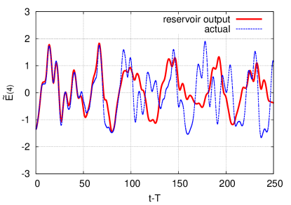
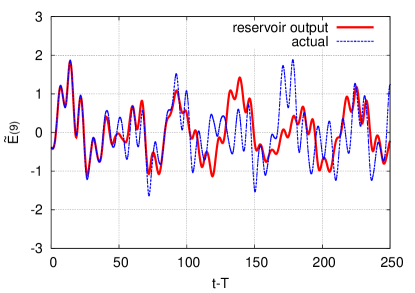
Figure 2: Full-inference of time-series of macroscopic variables of a fluid flow. Time-series of energy function ${\tilde{E}}(k,t)$ for $k=4$ (top) and $9$ (middle) are inferred from the reservoir system in comparison with that of a reference data obtained by the direct numerical simulation of the Navier–Stokes equation. The inference error defined by $\varepsilon(t)=\sum^{N_{0}}_{k=1}|\tilde{E}(k,t)-\hat{\tilde{E}}(k,t)|/N_{0}$ $(N_{0}=9)$ is shown to grow exponentially with time up to $t-T=100$ (bottom), which is inevitable for a chaotic behavior of a fluid flow. The growth of error within a short time highly depends on the direction of the perturbation vector $\{\tilde{E}(\cdot,T+\Delta t)-\hat{\tilde{E}}(\cdot,T+\Delta t)\}$, and its slope can vary in different settings.

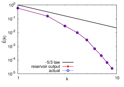
Figure 3: Energy spectrum $\overline{E}(k)$ reproduced from the reservoir computing. The spectrum is obtained from the full-inference of an energy function $E(k,t)$, which is compared with that for a reference data obtained by the direct numerical simulation of the Navier–Stokes equation. The coincidence of the two energy spectra implies that the reservoir system captures the dynamics of a fluid flow in statistical sense, even after the time-series inference has failed due to the chaotic property (see Fig. 2). The Kolmogorov $-5/3$ law of the energy spectrum is shown as a reference. The relative error of inferred variable $\overline{\hat{E}}(k)$ from $\overline{E}(k)$ $(k=1,\cdots,9)$ is up to $1.3\%$.

V V. Full-inference of macroscopic variables: Energy function and Energy spectrum

We study an energy function as the representative of a macroscopic variable. We set $\nu=0.058$ for which the flow is more turbulent than the previous case. However, the complexity of the dynamics is much less than that for a microscopic variable for the same viscosity. This is because the energy function can be thought of as an averaged quantity of many microscopic variables. The energy function $E_{0}(k,t)$ for wavenumber $k\in\mathbb{N}$ is defined by

$$E_{0}(k,t):=\dfrac{1}{2}\int_{D_{k}}{\sum_{\zeta=1}^{3}}\left|\mathcal{F}_{[v_{\zeta}]}(\kappa,t)\right|^{2}d\kappa,$$

where $D_{k}:=\{\kappa\in\mathbb{Z}^{3}|k-0.5\leq|\kappa|<k+0.5\}$. See eq. (5) for the expression of $\mathcal{F}_{[v_{\zeta}]}(\kappa,t)$. In order to get rid of the high-frequency fluctuation, we take the short-time average

$$E(k,t)=\sum_{s=t-99\Delta s}^{t}E_{0}(k,s)/100,$$

where $\Delta s=0.05$ is the time step of the integration of the Navier–Stokes equation. This helps us to obtain essential low-frequency dynamics of an energy function and infer its time-series with less computational costs with lower dimension $N$ of the reservoir vectors. The averaged energy function $E(k,t)$ will be called an energy function hereafter.
In the training phase for $t\in(0,T]$, $\mathbf{W}^{*}_{\text{out}}$ and $c^{*}$ are determined by setting

$$\mathbf{u}(t) =(\tilde{E}(1,t),\tilde{E}(2,t),\cdots,\tilde{E}(9,t))^{t},$$

$$\mathbf{s}(t) =(\tilde{E}(1,t),\tilde{E}(2,t),\cdots,\tilde{E}(9,t))^{t},$$

and by following the same procedure as the partial-inference. In the inference phase for $t>T$, eq.(1) is written as

$$\mathbf{r}(t+\Delta t)=(1-\alpha)\mathbf{r}(t)+\alpha\tanh(\mathbf{A}\mathbf{r}(t)+\mathbf{W}_{\text{in}}\hat{\mathbf{s}}(t)),$$

by setting $\mathbf{u}(t)$ as

$$\hat{\mathbf{s}}(t)=(\hat{\tilde{E}}(1,t),\hat{\tilde{E}}(2,t),\cdots,\hat{\tilde{E}}(9,t))^{t}$$

obtained from eq. (4). A set of parameters employed here is shown in TABLE 1 (b).
We found that an inference of energy functions is successful for some time after finishing training $9$-dimensional time-series data of energy functions. The two cases for $\tilde{E}(4,t)$ and $\tilde{E}(9,t)$ are shown in Fig. 2 (top)(middle). The failure in the long-term time-series inference is inevitable just due to the sensitive dependence on initial condition of a chaotic property of the fluid flow. In fact, the growth rate of error in the energy functions is shown to be exponential for $t-T\lesssim 100$ in Fig. 2 (bottom). However, the energy spectrum $\overline{E}(k)=\langle E(k,t)\rangle$, the time average of an energy function $E(k,t)$, can be reproduced from the inferred time-series data for $1000<t-T<2000$ (Fig. 3). This implies that the reservoir system constructed without the knowledge of microscopic variables captures statistical property correctly, and that the obtained system can be understood as a chaotic dynamical system describing a behavior of energy functions.

VI VI. Full-inference of Macroscopic variable from only one measurement using delay coordinates

In various experiments and observations of high-dimensional complex phenomena, there are usually much smaller number of measurements than the Lyapunov dimensions of the attractor. Even in such cases we can infer a time-series data by generating high-dimensional input data $\mathbf{u}$ for the reservoir computation through the delay-coordinate embedding method Takens (1981); Sauer et al. (1991).
Here we exemplify a full-inference of an energy function $E(4,t)$ for the same flow as in Section V, by assuming that the accessible measurement is limited to only one variable $E(4,t)$ among $9$ measurements $E(k,t)~{}(k=1,\cdots,9)$ used in Section V. In order to overcome the lack of sufficiently large number of measurements, we introduce $36$-dimensional delay-coordinate function with a time delay $\Delta\tau=2.5$, that is,

$$\mathbf{u}(t) =(\tilde{E}(4,t),\tilde{E}(4,t-\Delta\tau),\cdots,\tilde{E}(4,t-35\Delta\tau))^{t},$$

$$\mathbf{s}(t) =(\tilde{E}(4,t),\tilde{E}(4,t-\Delta\tau),\cdots,\tilde{E}(4,t-35\Delta\tau))^{t}.$$

An inferred time-series of $\tilde{E}(4,t)$ is shown in Fig. 4, which is as successful as the case when there are $9$ measurements in Fig. 2 (top). A set of parameters employed here is shown in TABLE 1 (c).

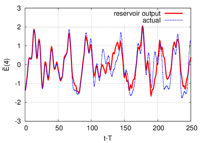
Figure 4: Full-inference of a macroscopic variable using the delay coordinates of only one measurement. We infer an energy function ${\tilde{E}}(4,t)$ for the same time range as in Fig. 2 (top) from only one measurement ${\tilde{E}}(4,t)$. The inferred time-series of ${\tilde{E}}(4,t)$ is shown together with a reference data obtained by the direct numerical simulation of the Navier–Stokes equation (top). Errors for the inference $\varepsilon_{1}(t)=\sum^{35}_{n=0}|\tilde{E}(4,t-n\Delta\tau)-\hat{\tilde{E}}(4,t-n\Delta\tau)|^{2}/36$ and $\varepsilon_{2}(t)=|\tilde{E}(4,t)-\hat{\tilde{E}}(4,t)|$ are shown (bottom).

VII VII. Discussion and remarks

We have succeeded in inferring time-series of both microscopic and macroscopic variables of a three-dimensional fluid flow by machine-learning technique using reservoir computing. The method is especially useful in generating an arbitrarily long time-series data of macroscopic variables as well as a statistical property with small computational costs. That is, in order to generate a time-series data of a macroscopic variable of a fluid flow, we do not need to refer microscopic behaviors. It takes roughly $1/80$ of time to obtain a time-series of the energy functions $E(k)$ with the same time-lengths, when we use the model constructed by the reservoir computation. The Navier–Stokes equation is calculated by 13718-dimensional ODEs with the $4$-stage Runge–Kutta method (time step $0.05$), whereas the model is calculated by 3200-dimensional map whose iterate corresponds to the time step $0.25$.
The difficulty in the construction of a reservoir model can vary mainly depending on the viscosity $\nu$. As the degree of turbulence increases by decreasing $\nu$, longer training time $T$ and higher dimension $N$ of the reservoir state vector $\mathbf{r}\in\mathbb{R}^{N}$ are required. However, for macroscopic variables the construction is relatively easy, even when the flow is turbulent. Because the degree of instability of a macroscopic behavior is relatively low in comparison with that of a microscopic behavior.
It is expected that our procedure will work, even if a high-frequency noise is added to the training data, because even in our current computation we have applied a low-pass filter for the inference of macroscopic variables. Although our approach focuses on constructing a model for a fluid flow with a fixed parameter $\nu$, it will be very interesting to consider a framework of the construction of a model with a parameter.
When we do numerical computation of the Navier–Stokes equation, we employ some discretized expressions using Fourier spectrum method, finite difference method and finite element method. The obtained reservoir system constructed from data can be understood as one of such expressions, describing a macroscopic (or a microscopic) dynamics of a fluid flow.
It is known that there is a difficulty in obtaining a closed form equation of macroscopic behavior of a fluid flow from the Navier–Stokes equation analytically, so called a “closure problem”. That is, in order to express the dynamics of the $n$-th moment variables, the $n+1$-th moment variables are required for any positive integer $n$. Our study on the data-driven modeling may give us insights on this kind of problem. For a relatively large value of $\nu$ considered in our paper, $\{E(k)\}_{k=1}^{K}$ seems to be enough for representing the dynamics of $E(k)$, whereas $\{E(k)\}_{k=1}^{K}$ will not be enough for more turbulent case with a smaller value of $\nu$, even if $K$ is chosen large enough. In such a case time-delay variables can be used for generating high-dimensional input data as are used in Section VI.

VIII Acknowledgements

We would like to thank anonymous referees for the critical reading of the manuscript and giving us some insightful comments to improve our paper. KN was supported by the Leading Graduate Course for Frontiers of Mathematical Sciences and Physics (FMSP) at the University of Tokyo. YS was supported by the JSPS KAKENHI Grant No.17K05360 and JST PRESTO JPMJPR16E5. Part of the computation was supported by the Collaborative Research Program for Young $\cdot$ Women Scientists of ACCMS and IIMC, Kyoto University.

References

- Snyder et al. (2012) J. C. Snyder, M. Rupp, K. Hansen, K.-R. Müller, and K. Burke, Phys. Rev. Lett. 108, 253002 (2012).
- Gabbard et al. (2018) H. Gabbard, M. Williams, F. Hayes, and C. Messenger, Phys. Rev. Lett. 120, 141103 (2018).
- Mills and Tamblyn (2018) K. Mills and I. Tamblyn, Phys. Rev. E 97, 032119 (2018).
- Hornik et al. (1989) K. Hornik, M. Stinchcombe, and H. White, Neural Networks 2, 359 (1989).
- Cybenko (1989) G. Cybenko, Mathematics of control, signals and systems 2, 303 (1989).
- Ling et al. (2016) J. Ling, A. Kurzawski, and J. Templeton, J. Fluid Mech. 807, 155 (2016).
- Kutz (2017) J. N. Kutz, J. Fluid Mech. 814, 1 (2017).
- Gamahara and Hattori (2017) M. Gamahara and Y. Hattori, Phys. Rev. Fluids 2, 054604 (2017).
- Hochreiter and Schmidhuber (1997) S. Hochreiter and J. Schmidhuber, Neural computation 9, 1735 (1997).
- Wan et al. (2018) Z. Y. Wan, P. Vlachas, P. Koumoutsakos, and T. Sapsis, PloS one 13, e0197704 (2018).
- Vlachas et al. (2018) P. R. Vlachas, W. Byeon, Z. Y. Wan, T. P. Sapsis, and P. Koumoutsakos, Proceedings of the Royal Society of London A: Mathematical, Physical and Engineering Sciences 474, 20170844 (2018).
- Verstraeten et al. (2007) D. Verstraeten, B. Schrauwen, M. D’Haene, and D. A. Stroobandt, Neural Network 20, 391 (2007).
- Inubushi and Yoshimura (2017) M. Inubushi and K. Yoshimura, Scientific Reports 7, 10199 (2017).
- Lu et al. (2017) Z. Lu, J. Pathak, B. Hunt, M. Girvan, R. Brockett, and E. Ott, Chaos 27, 041102 (2017).
- Pathak et al. (2017) J. Pathak, Z. Lu, B. Hunt, M. Girvan, and E. Ott, Chaos 27, 121102 (2017).
- Ibáñez-Soria et al. (2018) D. Ibáñez-Soria, J. Garcia-Ojalvo, A. Soria-Frisch, and G. Ruffini, Chaos 28, 033118 (2018).
- Pathak et al. (2018) J. Pathak, B. Hunt, M. Girvan, Z. Lu, and E. Ott, Phys. Rev. Lett. 120, 024102 (2018).
- Antonik et al. (2018) P. Antonik, M. Gulina, J. Pauwels, and S. Massar, Phys. Rev. E 98, 012215 (2018).
- Jaeger (2001) H. Jaeger, GMD Report 148, 13 (2001).
- Jaeger and Haas (2004) H. Jaeger and H. Haas, Scince 304, 78 (2004).
- Maass et al. (2002) W. Maass, T. Natschläger, and H. Markram, Neural Computation 14, 2531 (2002).
- Lu et al. (2018) Z. Lu, B. R. Hunt, and E. Ott, Chaos 28, 061104 (2018), https://doi.org/10.1063/1.5039508 .
- Lukosevivcius and Jaeger (2009) M. Lukosevivcius and H. Jaeger, Computer Science Review 3, 127 (2009).
- Ishioka (1999) K. Ishioka, “ispack-0.4.1,” http://www.gfd-dennou.org/arch/ispack/, (1999), GFD Dennou Club.
- Takens (1981) F. Takens, in Dynamical systems and turbulence, Warwick 1980 (Coventry, 1979/1980), Lecture Notes in Math., Vol. 898 (Springer, Berlin-New York, 1981) pp. 366–381.
- Sauer et al. (1991) T. Sauer, J. A. Yorke, and M. Casdagli, J. Stat. Phys. 65, 579 (1991).