The VIMOS Public Extragalactic Redshift Survey (VIPERS)

Abstract

Aims. Various galaxy classification schemes have been developed so far to constrain the main physical processes regulating evolution of different galaxy types. In the era of a deluge of astrophysical information and recent progress in machine learning, a new approach to galaxy classification has become imperative.

Methods. In this paper, we employ a Fisher Expectation-Maximization (FEM) unsupervised algorithm working in a parameter space of 12 rest-frame magnitudes and spectroscopic redshift. The model (DBk) and the number of classes (12) were established based on the joint analysis of standard statistical criteria and confirmed by the analysis of the galaxy distribution with respect to a number of classes and their properties. This new approach allows us to classify galaxies based on only their redshifts and ultraviolet to near-infrared ($UV-NIR)$ spectral energy distributions.

Results. The FEM unsupervised algorithm has automatically distinguished 12 classes: 11 classes of VIPERS galaxies and an additional class of broad-line active galactic nuclei (AGNs). After a first broad division into blue, green, and red categories, we obtained a further sub-division into: three red, three green, and five blue galaxy classes. The FEM classes follow the galaxy sequence from the earliest to the latest types, which is reflected in their colours (which are constructed from rest-frame magnitudes used in the classification procedure) but also their morphological, physical, and spectroscopic properties (not included in the classification scheme). We demonstrate that the members of each class share similar physical and spectral properties. In particular, we are able to find three different classes of red passive galaxy populations. Thus, we demonstrate the potential of an unsupervised approach to galaxy classification and we retrieve the complexity of galaxy populations at $z\sim 0.7$, a task that usual, simpler, colour-based approaches cannot fulfil.

1 Introduction

The problem of classification of galaxies and dividing them into different types is as old as the notion of ”extragalactic nebulae” (Hubble 1926). As Sandage et al. (1975), and more recently Buta (2011) and Buta & Zhang (2011) point out, classification of objects is the first step in the development of most sciences, and applies to galaxy studies no less than to any field of research. Only once we find common features of studied objects and use them to sort them into categories, do we obtain a starting point for the further analysis. Identifying similarities and differences between the selected groups allows us to then build theoretical models, which can ultimately lead us to the global picture of physical mechanisms at the origin of their properties.

Galaxies in the local Universe display a variety of shapes and structural properties. The main classification system still in use is the Hubble tuning fork diagram (Hubble 1926, 1936), with all the refinements introduced by Sandage (1961) and de Vaucouleurs (1959), based on the morphological properties of galaxies (see van den Bergh 1998; Buta 2011, for a detailed discussion). In the modern context, we alternatively refer to continuity of types in the morphological parameter space, where numerous morphological features are taken into account (Lintott et al. 2008, 2011; Buta et al. 2010; Kartaltepe et al. 2015). The basic Hubble classification of galaxies into ”early” and ”late” types (and their subtypes) has survived because, among other reasons, these types correlate well with other properties of galaxies, such as colours, stellar content, neutral hydrogen content and so on. (Kennicutt 1992; Roberts & Haynes 1994; Buta et al. 1994; Strateva et al. 2001; Deng 2010; Moutard et al. 2016a).

Indeed, many types of galaxy properties display bimodal distributions: photometric parameters, such as colours (e.g. Bell et al. 2004; Balogh et al. 2004b; Baldry et al. 2006; Franzetti et al. 2007; Taylor et al. 2015), morphological parameters like the Sérsic index (e.g. Sérsic 1963; Strateva et al. 2001; Driver et al. 2006; Krywult et al. 2017), the strength of spectral features (e.g. Balogh et al. 2004a; Kauffmann et al. 2003; Siudek et al. 2017) and so on. Therefore, these properties are often used as the basis for galaxy classification, especially at higher redshifts, $z$, where detailed galaxy morphologies are difficult to observe. In particular, colour-colour diagrams (e.g. the $(NUV-r)-(r-K)$ diagram (hereafter: $NUVrK$), $NURrJ$, $BzK$, $NUViB$, introduced/used by Arnouts et al. 2013; Bundy et al. 2010; Daddi et al. 2004; Cibinel et al. 2013, respectively) are often used for the purpose of galaxy classification. More refined selection processes can be based on the multi-modality criterion, which selects red passive galaxies, intermediate ”green valley” objects, and blue star-forming galaxies based on their rest-frame colours, spectral parameters, or colour and colour-Sérsic index distributions simultaneously (e.g. Bell et al. 2004; Baldry et al. 2006; Franzetti et al. 2007; Bruce et al. 2014; Lange et al. 2015; Krywult et al. 2017; Haines et al. 2017). The bimodality criterion can be enriched by a variable cut in galaxy colours that evolves with redshift (Peng et al. 2010; Fritz et al. 2014; Moutard et al. 2016b; Siudek et al. 2017), as a non-evolving cut applied for high-redshift galaxies can result in the selection of the reddest and most luminous red-type galaxies in one group and a mixture of star-forming and less massive red galaxies in the second group.

The methods presented above are powerful tools, but they are sensitive only to a few specific properties. A disadvantage of the methods presented above is the small number of groups which can typically be obtained: selection based on bimodality of the distribution of a certain property or a set of correlated properties usually allows for selection of only two or three groups (blue star-forming galaxies – intermediate types – red passive galaxies). Some two-dimensional (2D) colour-colour diagrams, like the $NUVrK$, are used for a more detailed classification (e.g. Arnouts et al. 2013; Moutard et al. 2016a, b; Davidzon et al. 2016) but are still limited to a relatively small number of groups.

Moreover, classifications based on the standard 2D cuts suffer from multi-fold selection-effect problems. For example, the properties of red passive galaxies selected using different criteria (photometry, morphology, and spectroscopy) differ from one selection to another (e.g. Renzini 2006; Moresco et al. 2013). Red passive galaxy samples are mostly affected by some level of contamination from dust-reddened galaxies with relatively low levels of star formation activity that may strongly affect their mean properties. Moresco et al. (2013) showed that the selection of the purest sample of red passive galaxies demands the combination of different criteria (in this case, morphological, spectroscopic and photometric information) confirming the necessity of multidimensional approaches in order to avoid obtaining a biased sample of different galaxy types.

Two-dimensional diagrams based on the flux ratios (or equivalent widths) of spectral lines can also be a powerful tool, for example for AGN diagnostic and classification (e.g. Baldwin, Phillips & Terlevich ”BPT” diagrams based on the ratios of ”blue” and ”red” lines: Baldwin et al. 1981; Lamareille 2010). The BPT diagram allows for separation of: (1) star-forming galaxies, (2) Seyferts, (3) low-ionisation nuclear emission-line regions (LINERS), and the two composite groups, which consist of: (4) star-forming galaxies and Seyferts, and (5) star-forming galaxies and LINERS.

However, it becomes clear that any classification based on a small number of parameters, even carefully chosen, is far too simple to reflect the huge range of different cosmic objects.

While classical methods of classification are still common and very useful, recent advancements in automatic machine learning have opened up new possibilities for the classification of distant sources. In principle, they allow us to operate in a multi-parameter space, combining all the available pieces of information: photometric measurements, redshifts, spectral lines, and morphologies. In principle, such an approach can immensely improve the galaxy classification across a wide redshift range. However, there is also a risk of including too much redundant or indiscriminative information which would blur the final result or lead to the unjustified subdivision of types.

Ball & Brunner (2010) and Fraix-Burnet et al. (2015) gave a comprehensive review of different methods for clustering objects into synthetic groups in astrophysics, showing that classification in multi-dimensional parameter space, backed by sophisticated multivariate statistical tools, leads to a selection of sources that is more accurate than, for example, the colour-colour method. In general, we can distinguish two main groups of algorithms: supervised and unsupervised learning algorithms.

Briefly, supervised algorithms classify data into classes that have previously been defined and anticipated. The disadvantage of this method is the requirement to create a training sample a priori and, at the same time, no possibility to define new classes of objects. Unsupervised learning algorithms (such as those used in our analysis) search for clusters of objects characterised by some pattern in the data and try to discover new classification schemes without any prior assumptions. The unsupervised algorithm fits the input vector data to a statistical model. The algorithm then tries to optimise the parameters of the model in iterative cycles to find the best fit to the data with an optimised number of classes. Once the defined satisfactory criteria are fulfilled, the iterations are stopped. The best known unsupervised learning algorithms include: (a) expectation-maximisation (Bilmes 1998, hereafter: EM) algorithms - used to deal with complex data structures, for example, clusters; (b) k-means (Salman et al. 2011) - whose aim is to assign observations to clusters in which each observation belongs to the nearest mean; and (c) hierarchical clustering (Balcan et al. 2014) - treating each point as a cluster and successively merging pairs of clusters recursively until all clusters are merged into one single group that contains all of the points. An overview of unsupervised approaches used in astronomy can be found in D’Abrusco et al. (2012).

Supervised algorithms have already yielded clear achievements in the selection of different astronomical sources. However, this approach only allows us to reproduce standard classifications, mostly based on optical colours, which is not optimal to extract all the relevant information from the data. Therefore, it is necessary to adopt unsupervised methods to efficiently extract all the information encoded in the data. The applications of unsupervised machine-learning algorithms to galaxy classification have until now mainly been applied to galaxy spectra. In particular, Sánchez Almeida et al. (2010) used an unsupervised k-means cluster analysis algorithm to classify all spectra in the final Sloan Digital Sky Survey data release 7 (SDSS/DR7). They identified as many as 17 different classes of galaxies. This would have been extremely challenging using classical methods due to the huge number of spectra ($\sim$174k) to process. The classification was based on the multidimensional cuts in the space of a mixture of features (emission/absorption lines, continuum, fluxes and errors) making use of 3849 measurements for each object. The selected classes are well separated in the colour sequence and morphological groups. The spectroscopic templates obtained for each class can be used for redshift measurements ($z<0.25$) as well as to trace morphological and spectroscopic changes in cosmic time.

Principal component analysis (PCA) has been used to classify astronomical data based on broadband measurements or as a tool to clean spectra (e.g. Marchetti et al. 2013; Wild et al. 2014; Marchetti et al. 2017). Marchetti et al. (2013) used a PCA algorithm to classify 27,350 optical spectra in the redshift range $0.4<z<1.0$ collected by the VIPERS survey (Public Data Release 1, hereafter PDR1). The algorithm repaired parts of VIPERS spectra affected by noise or sky residuals and reconstructed gaps in the spectra. A classification into four main classes (early, intermediate, late and starburst galaxies) was carried out, based on a set of orthogonal spectral templates and the three most significant components (eigen-coefficients) obtained for each galaxy.

In this paper, we introduce a new method of galaxy classification via an unsupervised learning algorithm applied to the galaxies observed by the VIMOS Public Extragalactic Redshift Survey (VIPERS). The VIPERS survey acquired spectra for $\sim 10^{5}$ galaxies. For each galaxy, both spectroscopic measurements (redshift, lines, fluxes) and photometric data are provided. This makes VIPERS a perfect dataset for unsupervised classification; it is large enough to separate many different classes on a statistically sound level, and, at the same time, all the wealth of the spectroscopic and photometric information can be used to construct the feature space, and later for the validation process. Moreover, previous analyses made on the VIPERS data provide us with additional parameters such as Sérsic indices and physical properties, obtained by fitting the spectral energy distributions (SEDs) (stellar mass, star formation rate (SFR), etc.). All these additional measurements, even when not used for the classification itself, can serve for an a posteriori interpretation of physical properties of different classes. Our method is based on the multidimensional space defined by the rest-frame luminosities measured in 12 bands and, additionally, spectroscopic redshift information.

The availability of spectroscopic data for VIPERS galaxies allows us to verify how the classes obtained using the broadband rest-frame photometry are reflected in the spectral properties of galaxies. We demonstrate that the classification based on our automatic algorithm and confirmed by spectroscopic features provides a homogeneous view of different classes of galaxies which may be used as the starting point to analyse their evolutionary tracks leading to the formation of today’s galaxy types.

The paper is organised as follows. In Sect. 2, we describe the sample selection. Section 3 gives an overview of the FisherEM methodology. In Sect. 4, we present the main results and discuss their physical meaning. A summary is presented in Sect. 5. We validate the model and the number of classes in Appendix A, and discuss the class membership probabilities in Appendix B. We compared FEM classification to a principal component analysis (PCA) scheme in Appendix C, and relate FEM classes to Hubble types given by Kennicutt (1992) in Appendix D.

In our analysis, we used the free statistical environment software R3 with the FisherEM package 4 (Bouveyron & Brunet 2011). Throughout the paper we use a cosmological framework assuming $\Omega_{m}$ = 0.30, $\Omega_{\Lambda}$ = 0.70, and $H_{0}=70$ km s^-1 Mpc^-1.

2 Data

In this paper, we make use of the final galaxy sample from the VIMOS Public Extragalactic Redshift Survey (VIPERS, Scodeggio et al. 2018). VIPERS is a spectroscopic survey carried out with the VIMOS spectrograph (Le Fèvre et al. 2003) on the 8.2m ESO Very Large Telescope (VLT) aimed at measuring redshifts for $\sim$100,000 galaxies in the redshift range 0.5–1.2. VIPERS covered an area of $\sim$23.5 $\deg^{2}$ on the sky, observing galaxies brighter than $i_{AB}=22.5$ at redshifts higher than 0.5 (a pre-selection in the ($u$-$g$) and ($r$-$i$) colour-colour plane was used to remove galaxies at lower redshifts). A detailed description of the survey can be found in Guzzo et al. (2014). The galaxy target sample was selected from optical photometric catalogues of the Canada-France-Hawaii Telescope Legacy Survey Wide (CFHTLS-Wide: Mellier et al. 2008; Goranova et al. 2009). The data reduction pipeline and redshift quality system are described by Garilli et al. (2014).

2.1 The VIPERS dataset

The final data release provides spectroscopic measurements and photometric properties for 86,775 galaxies (Scodeggio et al. 2018). The associated photometric catalogue consists of magnitudes from the VIPERS Multi-Lamba Survey (Moutard et al. 2016a), combining CFHTLS T0007-based $u$, $g$, $r$, $i$, $z$ photometry with GALEX $FUV$/$NUV$ and WIRCam $Ks$-band observations, complemented where available by VISTA $Z$, $Y$, $J$, $H$, $K$ photometry from the VIDEO survey (Jarvis et al. 2013).

Physical parameters including absolute magnitudes, stellar masses, and SFRs for the VIPERS sample were obtained via SED fitting with the code LePhare (Arnouts et al. 2002; Ilbert et al. 2006). The whole multi-wavelength information available in the VIPERS fields (from $UV$ to $NIR$) was used, applying the Bruzual & Charlot (2003) models and three extinction laws. In addition, absolute magnitudes were computed using the nearest observed-frame band in order to minimise the dependence on models. The detailed description of the VIPERS data SED-fitting scheme that we adopted in the present analysis can be found in Moutard et al. (2016b).

In this work, we make use of the subset of galaxies with highly secure redshift measurements (with a confidence level higher than 99%, i.e. with redshift flag 3–4 and 13–14, see Garilli et al. 2014, for details). This subset contains 52,114 objects (51,522 galaxies and 592 broad-line AGNs). They are observed in the redshift range $0.4<z<1.3$ with a mean (median) redshift of 0.7.

2.2 The multidimensional feature data

Data preparation is a key issue in working with learning algorithms, both supervised and unsupervised. In order to minimise any biases, maximise homogeneity in the input data, and use all of the available information, 12 rest-frame magnitudes are chosen: $FUV$, $NUV$, $u$, $g$, $r$, $i$, $z$, $B$, $V$, $J$, $H$, and $Ks$ derived from the SED fitting (see Sect. 2, and Moutard et al. 2016b), as well as the spectroscopic redshift (Scodeggio et al. 2018). To avoid grouping galaxies based on differences in their luminosities instead of differences in their SEDs, the data were standarised. We normalised $i$-band to unity and transformed each absolute magnitude by the normalisation factor (the redshifts were not transformed as their values are already around unity). This allowed us to code the data into common numerical range preventing the algorithm from splitting our sample along any direction with extended amplitudes.

The normalised parameters, together with the spectroscopic redshift, are then used to create a multi-parameter space for the FEM algorithm. The spectroscopic redshift is included in the parameter space to make the classification sensitive to possible evolutionary changes with cosmic time. The algorithm could identify an evolving population in different cosmic epochs as belonging to physically different classes. Although this is not the case for the VIPERS galaxies, where all FEM classes seem to be preserved throughout the redshift range probed by the survey (see Sect. 4), we did not want to exclude this option a priori. However, we verified that if the spectroscopic redshift is not included in the parameter space, the FEM classification remains practically the same.

The global picture of the classification does not suffer significantly if we reduce the feature space by one parameter (e.g. spectroscopic redshift). However, excluding each single feature has an impact on the ability of the algorithm to distinguish individual classes. Feature importance may be statistically determined by the analysis of the orientation of the discriminative subspace. The x-axis of a hyperplane separating classes in a latent subspace is constructed with an 11-degree polynomial and each coefficient describes how important each feature is for the distinction of each group. For example, high coefficients of the hyperplane between red passive classes for $FUV$ and $NUV$ reveal their importance in distinguishing those groups. Therefore, excluding $FUV$ and $NUV$ will result in discriminating ten classes with only one large red passive class leaving the remaining classes unchanged. The redundancy of selected features and their importance to distinguish each group will be further discussed by Krakowski et al. (in prep).

We note that the redundancy of the spectroscopic redshift reveals a great potential for future photometric missions such as Euclid and LSST. In Siudek et al. (2018), we explore the potential use of photometric information solely to classify galaxies and estimate their properties. Reliable photometric redshifts and 12 rest-frame magnitudes obtained by the SED-fitting with the photo-z scatter $\sigma\sim 0.03$, and the outlier rate $\mu\sim 2\%$ obtained for the VIPERS sample, were used to verify how precisely the detailed classification could be reproduced if only photometric data were available. The confirmed accuracy in recreating galaxy classes: 92%, 84%, 96% for red, green, and blue classes, respectively , together with the ability to efficiently separate outliers (stars and broad-line AGNs) based only on photometric data, demonstrates the potential of our approach in future large cosmology missions to distinguish different galaxy classes at $z>0.5$.

3 Method – Fisher EM

Unsupervised learning algorithms are used to divide the data of a priori unknown properties into clusters. In this paper, we use the FEM (Bouveyron & Brunet 2011) algorithm, which is an extension of the EM algorithm. The main goal of both the EM and the FEM classifiers is to maximise the best fit of the chosen statistical model describing the data by finding the optimal parameters of this model. In the case of the FEM algorithm, the main assumption is that the data can be grouped into a common discriminative latent subspace which is modelled by the discriminant latent mixture (hereafter: DLM) model (Bouveyron & Brunet 2011). This discriminative latent subspace is defined by linear combinations of the input data (latent variables; Bouveyron & Brunet-Saumard 2014). It is then optimised to maximise the separation between groups and minimise their variance at the same time. The second assumption of the FEM algorithm is that our data can be separated into an a priori unknown number of groups, each described by a Gaussian profile in the multidimensional parameter space. The role of the FEM algorithm is to find the best fit of these multi-Gaussian profiles to the data, optimising both the number of the groups and their location in the parameter space.

3.1 The performance of the FEM algorithm

Unsupervised learning algorithms start by assigning initial cluster (class) centres, that is, galaxies representative of a given class. To select the optimal centre points, they are iteratively changed by assigning either (1) random values, or (2) pre-defined values obtained from another simpler and faster clustering algorithm. This is an essential step as classification algorithms yield different classes with each random initialisation, while we want to obtain final classification results that are as stable as possible. The randomised initialisation is fraught with the risk of finding a local probability minimum, which results in the erroneous assignment of objects to groups. In order to avoid such a situation, a random procedure for assigning initial values of function parameters can be repeated several times, and then the model with the highest log-likelihood is selected. However, to achieve optimal cluster centres, the number of random values needs to be equal to the number of galaxies.

The second approach described above is the one applied in our analysis; in particular, for the choice of the initial values, the k-means++ algorithm is used (Arthur & Vassilvitskii 2007) to obtain the optimal cluster centres. This algorithm starts from a random choice of cluster centres among the data points. It then estimates the distances of all data points from these centres, and based on a weighted probability proportional to these squared distances, it selects new centres. This procedure is repeated until the choice of centres does not change with the next realisation, i.e. the optimal centres are found. Each initialisation gives a different classification, and each run groups similar galaxies into clusters, and so, in principle, all of them provide valuable classifications. The problem is then to select which classification is the best, i.e. which one should be chosen as the final classification. To overcome this issue, we run the k-means algorithm 15 times to find the optimal initial parameters. Moreover, this ensures that we obtain a representative classification, as we are able to recreate the divisions. As in Sánchez Almeida et al. (2010), the k-means algorithm could be used for classification purposes itself. However, it is not as sophisticated as FEM, as it demands a pre-defined number of clusters (classes) and it also suffers from the initialisation problem. Therefore, we used k-means as the first step to optimise the starting points for a more advanced tool.

Once the starting points of the algorithm have been selected, the FEM algorithm is executed assuming that: (1) the input parameters, magnitudes and redshift values, can be projected onto a latent discriminative subspace with a dimension lower than the dimension (K) of the observed data, and (2) this subspace (K-1) is sufficient to discriminate K classes. The algorithm then performs the E (expectation), F (Fisher criterion), and M (maximisation) steps described below that are repeated in each cycle.

In step E, the algorithm calculates the complete log-likelihood, conditionally to the current value of the Gaussian mixture model. In practice, this means the calculation of the probability of each considered object belonging to the groups predefined by the k-means++ algorithm.

In step F, the DLM model chooses the subspace $f$ in which the distances between groups are maximised and their internal scatter is minimised:

$$f=\frac{(\eta_{1}-\eta_{2})^{2}}{\sigma_{1}^{2}+\sigma_{2}^{2}},$$ (1)

where $\eta_{1}$ and $\eta_{2}$ are the mean values of the centres of the analysed groups, and $\sigma_{1}^{2}$ and $\sigma_{2}^{2}$ are their variances (Fukunaga 1990). The mean and variance are measured for each group in the observation space. The algorithm searches for a linear transformation U, which projects the observation into a discriminative and low-dimensional subspace d, such that the linear transformation U of dimension $p\times d$ (where p is the dimension of the original space) aims to maximise a criterion that is large when the between-class covariance matrix (SB) is large and when the within-covariance matrix (SW) is small. Since the rank of SB is at most equal to K – 1, where K is the number of classes, the dimension d of the discriminative subspace is therefore at most equal to K – 1 as well. For details, we refer to Sects. 2.4 and 3.1 in Bouveyron & Brunet (2012).

Subsequently, in step M, the parameters of the multivariate Gaussian functions are optimised, by maximising the conditional expectations of the complete log-likelihood, based on the values obtained in the previous steps (E+F).

The algorithm then comes back to step E, now computing the probabilities for each object to belong to groups modified in the last step M.

This procedure is repeated until the algorithm converges according to the stopping criterion which is based on the difference between the likelihoods calculated in the last two steps.

3.2 DLM models for the FEM algorithm

To perform the FEM analysis, it is necessary to choose a model and the number of groups. There exist different DLM models that have been created for different applications. Specific models differ in the numbers of components and their parameters. The variety of these models then allows them to fit into various situations. The 12 different DLM models are considered: DkBk, DkB, DBk, DB, AkjBk, AkjB, AkBk, AkBk, AjBk, AjB, ABk and AB. The main differences between them is in the number of free parameters left to be estimated (Bouveyron & Brunet 2011). In the primary model, DkBk, two components can be distinguished: Dk and Bk, where Dk is responsible for modelling the variance of the actual data (by parametrizing the variance of each class within the latent subspace), and Bk which models the variance of the noise (i.e. it parametrizes the variance of the class outside the latent subspace). The other models are in fact submodels of DkBk in which certain parameters of the Dk and Bk components are assumed to be common between and/or within classes. For example, the DBk model assumes that the variance in a latent subspace is common to all classes, whereas the DkB model assumes that the variance outside the latent subspace is common across classes. The combination of these two constraints (common variance inside and outside the latent subspace to all classes) results in the DB model. Therefore, these submodels are characterised by a lower number of parameters: if our thirteen-dimensional dataset is divided into 12 groups, the ”main” DkBk model would be characterised by 1,024 free parameters, while the DkB model would be characterised by 1,013 parameters, the DBk model by 298 parameters, the DB model by 287 parameters, down to the simplest AB model with 222 free parameters. The number of free parameters needed is dictated by the complexity of the input data and the mathematical equations given in Bouveyron & Brunet (2012). A highly parametrised model requiring the estimation of a large number of free parameters is preferred for clustering of high-dimensional data. We refer the reader to Bouveyron & Brunet (2012) for a detailed description of the DLM family. Comparing the performance and convergence of different models, we find that the VIPERS data are best parametrised by the DBk model with 298 free parameters.

3.3 The selection of the optimal model and number of classes

The number of classes is not known a priori, which is one of the major difficulties in applying unsupervised clustering algorithms to classify astronomical sources. Defining the optimal number and model is not trivial. We do not make any a priori assumptions about galaxy separation, that is, if the data could not be described by the DLM models, for example because of the non-Gaussian nature of the datasets, the FEM algorithm simply would not converge. In our work, the best DLM model and the range of possible class numbers is chosen based on three statistical model-based criteria: the Akaike Information Criterion (AIC; Akaike 1974), the Bayesian Information Criterion (BIC; Schwarz 1978) and the Integrated Complete Likelihood (ICL; Baudry 2012, see Appendix A). These are typical criteria used to evaluate statistical models (e.g. de Souza et al. 2017), which allow us to select the best model (DBk) and the approximate number of classes (9–12; see Appendix A). However, in order to pinpoint the diversity of physical properties among VIPERS galaxies, the final optimal number of classes is based on the flow of the galaxy distribution among a different number of classes (see Fig. 12) and their physical properties (see Fig. 1).

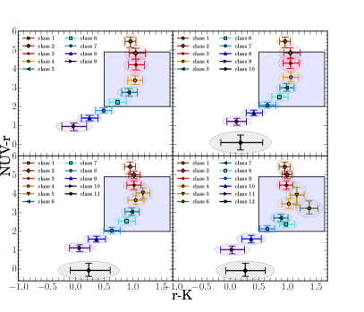
Figure 1: $NUVrK$ diagrams of FEM classes 9 – 12. The optimal number of classes was found to be 12. The error bars correspond to the first and the third quartile of the galaxy colour distribution, while the two half axes of the ellipses correspond to the median absolute deviation.

The analysis of the positions and properties of different classes on the $NUVrK$ diagrams allows us to verify if the classes do indeed reveal distinct physical properties. Figure 1 shows the $NUVrK$ diagrams for the classifiers consisting of 9, 10, 11 and 12 groups. As we can see in the figure, the division into groups for a different number of classes differs, especially in the region of dusty galaxies indicated by the shaded box. We can see the emergence of three new classes (classes 5, 6, 8) in the twelve-group division that were not distinguished by a lower number of clusters. The physical analysis of these classes (see Sect. 4) demonstrates that the classifier’s grasp of subtle differences between groups reveals these classes of dusty star-forming galaxies. Therefore, we find that division into 12 classes is physically motivated and this is also confirmed by analysis of the flow chart as all 12 classes are naturally separated from bigger groups, including separating broad-line AGNs from class 9 in the tenth iteration (see Fig. 12). We also found that with 13 classes, we obtain a worse classification, as the 13th class emerges from class 11 but does not represent different physical properties with respect to the 11th class (see Appendix A).

To summarise, using three statistical criteria: AIC, BIC, and ICL, we originally restricted the optimal number of classes to be between 9 and 12. After that, we checked the flow of galaxy distributions for realisations with different numbers of classes and their physical properties. We concluded that the optimal solution for classification of the VIPERS dataset is a DBk model with 12 classes (see Appendix A).

4 Results

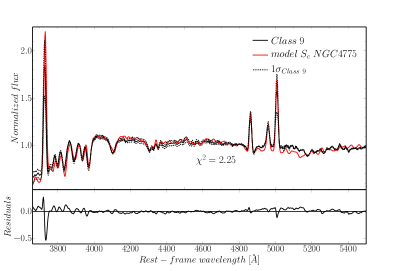
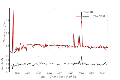
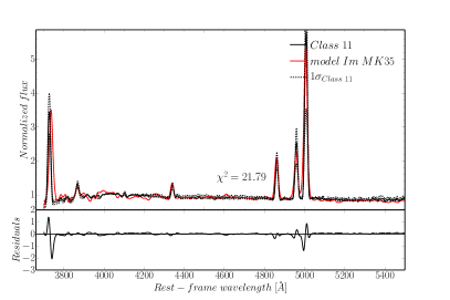
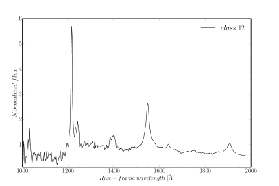
Figure 17: Continuation of Fig. 16. The composite spectrum of galaxies within the 12th class is built using only objects observed at $z\sim 2$. The wavelength range of spectra in the spectral atlas of Kennicutt (1992) does not cover the observed wavelength range.

In this section, the FEM classification of $z\sim 0.4-1.3$ galaxies is presented. We demonstrate that the 12 classes correspond to physically different and separate galaxy categories. In the following analysis, different properties of our classes are investigated to show that our classes actually mirror the sequence of galaxy types from the earliest (class 1) to the latest types (class 11) in the redshift range $0.4<z<1.3$. Classes 1–11 all have very similar redshift distributions (see Table 1), centred at $z\sim 0.7$, suggesting that these classes are persistent at least over the redshift range $0.4<z<1.3$. A different median redshift is measured within the 12th class. This class cannot be placed along the same sequence as the other classes. Class 12 mainly groups high-redshift VIPERS sources (with median redshift $z_{med}\sim 2$; see Table 1). Members of this group are mostly identified as broad-line AGNs according to their redshift flag (see Sect. 2; $\sim 95\%$, and Table 1). Therefore, class 12 is not part of the galaxy population at $z\sim 0.7$ that is the focus of this paper, and from now onwards only the first 11 galaxy classes will be discussed. The global properties of class 12 are presented in Table 1 and the composite spectrum is shown in Fig. 17, but it is not included in the remaining plots. The SED fitting procedure used for VIPERS sources does not include AGN templates. Therefore, the AGN host properties (stellar mass and SFRs, $r$-$K$ colour, as $K$ significantly depends on models) might be wrong. The classification was performed on the whole sample (i.e. including broad-line AGNs, even if they are not the focus of this paper) to demonstrate the global usefulness of the FEM algorithm and its ability to separate broad-line AGNs and galaxies. Although the algorithm was able to a separate a class of broad-line AGNs, only $\sim 50\%$ of broad-line AGNs at $z>1.3$ were assigned to this separate class, while the other half were spread among the star-forming classes 9–11. The fraction of broad-line AGNs in these classes is however negligible ($<5\%$ galaxies in a given class). This approach allows us to reproduce common classification schemes, which do not explicitly exclude any groups of sources. It should be noted that although class 12 can be expected to be separated based on the use of spectroscopic redshift as an input parameter, even when the redshift is not included in the parameter space (i.e. classification is based only on rest-frame colours) class 12 is reproduced with an accuracy of the order of $\sim 80\%$.

Table 1: The main physical properties of the FEM classes.

Class

$N$

$frac[\%]$

$z$

$n$

$NUV-r$

$r-K$

$U-V$

$D4000_{n}$

$EW(OII)$

$log(M_{star}/M_{\odot})$

$log(sSFR)[yr^{-1}]$

$N_{AGNs}$

$frac_{AGNs}[\%]$

(1)

(2)

(3)

(4)

(5)

(6)

(7)

(8)

(9)

(10)

(11)

(12)

(13)

(14)

Elliptical galaxies

1

4476

9.11

$0.67^{+0.11}_{-0.11}$

$3.33^{+0.96}_{-1.20}$

$5.43^{+0.37}_{-0.24}$

$0.95^{+0.10}_{-0.10}$

$1.99^{+0.09}_{-0.08}$

$1.76^{+0.11}_{-0.11}$

–

$10.77^{+0.24}_{-0.23}$

$-16.88^{+2.16}_{-3.55}$

0

0.00

2

2399

4.88

$0.67^{+0.10}_{-0.11}$

$3.32^{+1.03}_{-1.30}$

$5.04^{+0.19}_{-0.18}$

$0.99^{+0.08}_{-0.09}$

$1.98^{+0.09}_{-0.08}$

$1.75^{+0.12}_{-0.10}$

–

$10.83^{+0.21}_{-0.22}$

$-11.85^{+0.14}_{-0.29}$

0

0.00

3

3558

7.24

$0.68^{+0.10}_{-0.10}$

$3.04^{+0.99}_{-1.42}$

$4.46^{+0.22}_{-0.21}$

$0.98^{+0.12}_{-0.11}$

$1.91^{+0.10}_{-0.09}$

$1.68^{+0.14}_{-0.12}$

–

$10.83^{+0.23}_{-0.23}$

$-11.28^{+0.16}_{-0.17}$

0

0.00

Intermediate galaxies

4

4274

8.70

$0.70^{+0.11}_{-0.11}$

$1.78^{+0.68}_{-1.11}$

$3.47^{+0.24}_{-0.25}$

$1.03^{+0.12}_{-0.13}$

$1.64^{+0.14}_{-0.12}$

$1.41^{+0.11}_{-0.14}$

–

$10.69^{+0.25}_{-0.23}$

$-9.79^{+0.60}_{-0.47}$

4

0.09

5

3375

6.87

$0.63^{+0.08}_{-0.08}$

$2.07^{+0.77}_{-1.17}$

$3.93^{+0.51}_{-0.41}$

$1.17^{+0.12}_{-0.13}$

$1.82^{+0.21}_{-0.15}$

$1.50^{+0.15}_{-0.16}$

–

$10.50^{+0.27}_{-0.23}$

$-9.57^{+0.17}_{-0.33}$

0

0.00

6

964

1.96

$0.67^{+0.09}_{-0.09}$

$1.35^{+0.51}_{-0.81}$

$3.29^{+0.29}_{-0.38}$

$1.41^{+0.16}_{-0.14}$

$1.58^{+0.14}_{-0.20}$

$1.36^{+0.10}_{-0.11}$

$-16^{+7}_{-5}$

$10.50^{+0.21}_{-0.22}$

$-9.21^{+0.35}_{-0.42}$

2

0.21

Star-forming galaxies

7

5099

10.38

$0.67^{+0.11}_{-0.12}$

$1.15^{+0.40}_{-0.75}$

$2.71^{+0.19}_{-0.19}$

$0.88^{+0.12}_{-0.12}$

$1.35^{+0.14}_{-0.12}$

$1.28^{+0.07}_{-0.09}$

$-16^{+8}_{-5}$

$10.36^{+0.30}_{-0.31}$

$-9.29^{+0.45}_{-0.47}$

17

0.33

8

1755

3.57

$0.72^{+0.09}_{-0.10}$

$0.91^{+0.33}_{-0.70}$

$2.38^{+0.16}_{-0.15}$

$1.00^{+0.12}_{-0.14}$

$1.15^{+0.09}_{-0.08}$

$1.21^{+0.05}_{-0.06}$

$-21^{+9}_{-7}$

$10.12^{+0.23}_{-0.19}$

$-8.76^{+0.26}_{-0.30}$

14

0.80

9

5378

10.95

$0.67^{+0.11}_{-0.13}$

$0.92^{+0.30}_{-0.64}$

$2.13^{+0.16}_{-0.15}$

$0.63^{+0.12}_{-0.13}$

$1.07^{+0.13}_{-0.12}$

$1.21^{+0.06}_{-0.07}$

$-24^{+8}_{-7}$

$9.91^{+0.25}_{-0.28}$

$-8.95^{+0.43}_{-0.39}$

31

0.58

10

13978

28.45

$0.66^{+0.10}_{-0.12}$

$0.94^{+0.31}_{-0.63}$

$1.60^{+0.21}_{-0.19}$

$0.36^{+0.16}_{-0.18}$

$0.86^{+0.12}_{-0.11}$

$1.16^{+0.06}_{-0.06}$

$-36^{+10}_{-8}$

$9.56^{+0.22}_{-0.23}$

$-8.84^{+0.21}_{-0.28}$

123

0.88

11

2699

5.49

$0.71^{+0.12}_{-0.18}$

$1.11^{+0.45}_{-0.83}$

$1.01^{+0.21}_{-0.20}$

$0.03^{+0.20}_{-0.22}$

$0.59^{+0.14}_{-0.12}$

$1.07^{+0.07}_{-0.07}$

$-54^{+14}_{-12}$

$9.28^{+0.21}_{-0.25}$

$-8.61^{+0.33}_{-0.32}$

216

8.00

Broad-line AGNs

12

174

0.35

$2.24^{+0.25}_{-0.56}$

$2.80^{+1.17}_{-0.89}$

$-0.08^{+0.31}_{-0.39}$

*

$0.49^{+0.49}_{-0.31}$

$1.00^{+0.14}_{-0.16}$

–

*

*

166

95.40

As mentioned in Sect. 1, standard selection methods are powerful tools, but are however sensitive only to a few specific properties. We explored how such a refined classification compares with more standard two- or three-class division of galaxy population. The FEM classification separates VIPERS galaxies into eleven classes, which may be assigned to three wider galaxy categories: (1) red, passive, (2) green, intermediate, and (3) blue, star-forming. Since our classification was based on colours, the conventional nomenclature of red (classes 1–3), green (classes 4–6), and blue (classes 7–11) galaxies is applied (see Fig. 2(a), 2(b), and 2(c)). As the subsequent analysis demonstrates (Sect. 4.1, 4.2), the division between red (passive), green (intermediate), and blue (star-forming) galaxies is not sharp, as the intermediate groups (classes 3 and 7) are not purely passive or star-forming in terms of their global properties. Moreover, we note that a FEM classification into two or three main groups is not entirely unequivocal.

We compared our final eleven-class classification with a two-class FEM separation. The simple separation into two main clouds (red and blue) is able to distinguish a separate group of blue star-forming galaxies: $97\%$ of galaxies from classes 7–11 are assigned to the blue cloud and only $3\%$ of green galaxies (classes 4–6) were found in the blue cloud. At the same time, red and green galaxies are indistinguishable in the red cloud: $100\%$ of red galaxies (classes 1–3) were assigned to the red cloud, as were $97\%$ of green galaxies (classes 4–6).

In the subsequent step, the standard three-class (red/green/blue) division is compared with the FEM 11-class classification. As in the case of the two-class division, we are also not able to separate a red passive population from green galaxies. Almost all red galaxies assigned to classes 1–3 ($99\%$) were found in a red group. However, this group is strongly contaminated by green galaxies: $43\%$ of intermediate galaxies (classes 4–6) were found in the red cloud. The distinction between green and blue galaxies is also not obvious. Only $67\%$ of blue star-forming galaxies (classes 7–11) were assigned to the blue cloud, while the remaining $33\%$ were found within the green population.

For the two-class separation, red and green galaxies go together to form one group only, while for the three-class division, the green population is split between red and blue galaxies. This implies that the borderlines between green/blue and red/green populations are much less sharp than that for the eleven-class division. Only a more detailed classification can appropriately yield the division between red, green, and blue populations.

The FEM classification yielded distinct clusters in the thirteen-dimensional space, although the separation between classes is smooth. Some galaxies are close to the borders of different classes, and this is reflected in their lower posterior probabilities of being members of the class to which they are assigned. The posterior probability is correlated with the distance of the sources from the centre of the group in multidimensional space. There is no correlation of probabilities with the properties of the input data, that is, no dependence of the probability on the redshift measurement accuracy or luminosity was found. We assume that the classification, which assigns a probability of being a member of the class instead of a single class membership, should be a better approximation of the galaxy evolution, as a continuous transition between different groups (even if they are well separated in the feature space) is expected. Therefore, each group contains its core representative population and a (usually small) number of galaxies that are more loosely mapped to them. A detailed description of the class membership probabilities is given in Appendix B. In the following analysis, we focus on the representative galaxies, for which the class membership is not questionable. Our initial sample of 52,114 galaxies was therefore cleaned by excluding objects located in between adjacent classes, and outliers, based on their probability. In particular, 2,947 galaxies with low probabilities ($<50\%$) of being class members, and 1,038 objects with high ($>45\%$) probabilities of belonging to a second group were removed. However, it is worth noting that this leads to the rejection of only $8\%$ of the sample, therefore demonstrating the robustness of the clustering process performed with the FEM algorithm.

The resultant final catalogue consists of 47,556 galaxies (and 573 broad-line AGNs). The number of sources in each class, as well as the basic properties of the FEM classes, are summarised in Table 1.

4.1 Multidimensional galaxy separation versus standard methods

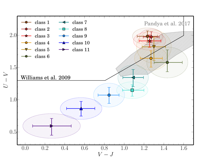
(a) $UVJ$ diagram;

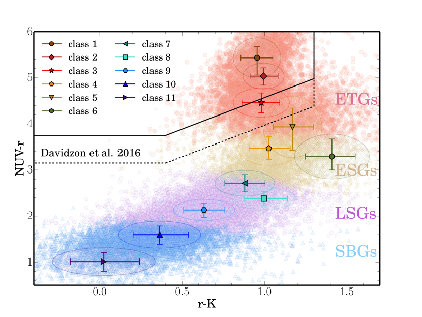
(b) $NUVrK$ diagram;

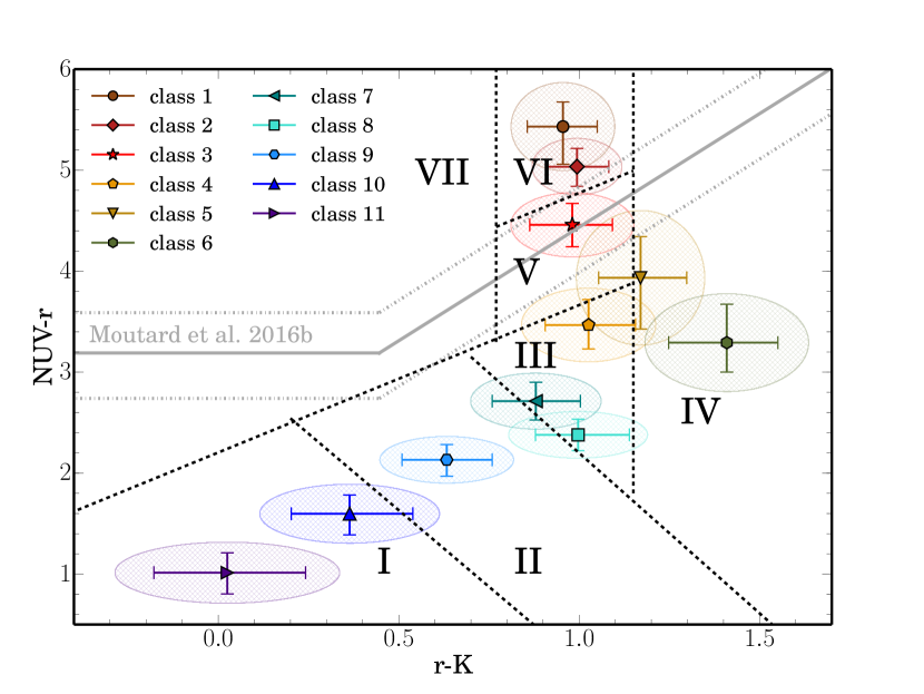
(c) $NUVrK$ diagram;

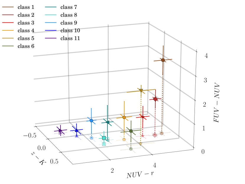
(d) 3D colour diagram;

Figure 2: Colour-colour(-colour) diagrams of the VIPERS galaxies classified into 11 classes with the FEM algorithm. The error bars correspond to the first and the third quartile of the galaxy colour distribution, while the two half axes of the ellipses correspond to the median absolute deviation. (a) The $UVJ$ diagram. The solid line corresponds to the standard separation between quiescent and star-forming galaxies. The area occupied by CANDELS transition galaxies is shown as a grey shaded area (Pandya et al. 2017). (b) The $NUVrK$ diagram. The black solid line corresponds to the separation of red passive galaxies, and the dotted line separates additionally galaxies located in green valley. Galaxies photometrically classified by their SED type as: (1) early-type (red E and Sa; ETGs), (2) early spiral (ESGs), (3) late spiral (LSGs), and (4) irregular or starburst (SBGs) following the prescription given in Fritz et al. (2014) are marked with light salmon, gold, violet, and blue, respectively. (c) The $NUVrK$ diagram. The black dashed lines corresponds to the division of CFHTLS galaxies into seven groups proposed by Moutard et al. (2016a). The grey solid line corresponds to the separation of red passive galaxies. The grey dash-dotted lines correspond to upper (lower) limits of the green valley galaxies proposed by Moutard et al. (2016b). (d) The 3D diagram. The dotted lines indicate the projection of FEM classes on the bottom plane ($z-K$ vs. $NUV-r$).

The FEM classification allows for a more sophisticated galaxy separation than the standard two-dimensional (2D) colour-colour diagrams. The typical classification schemes are mostly based on tight and linear cuts in the 2D space, while an unsupervised approach associates each object to the group based on its location in the multidimensional space describing galaxy properties. Colour-colour diagrams, including $NUVrK$ (Arnouts et al. 2013) and $U-V$ versus $V-J$ ($UVJ$; Williams et al. 2009), are coarser classifications than the ones obtained with the multidimensional approach, even if the trends are continuous. At the same time, the FEM classes correspond well to the classification schemes based on all these colour-colour diagrams. FEM classes are able to reproduce the standard colour-colour separation into passive and star-forming galaxies. Unsupervised classification further introduces the division into subclasses, which monotonously change their physical, spectroscopic, and morphological properties from class to class. This reveals the differences within passive, intermediate, and star-forming galaxy populations. The FEM classification creates a multidimensional separation cut. The advantage of this approach is that it is sensitive to a larger number of galaxy properties with respect to standard classification techniques. For example, as shown in a subsequent analysis, the three red passive classes are indistinguishable in the $r-K$, $U-V$, and $V-J$ colours, but have different $FUV$ and $NUV$ properties. Figure 2 presents colour-colour diagrams: $FUV-NUV$ versus $z-K$ versus $NUV-r$, $NUVrK$, and $UVJ$, where the median colours for the 11 FEM classes are shown. The error bars correspond to the first and third quartiles of the galaxy colour distribution, while the semi-major and minor axes of the ellipses correspond to the normalised median absolute deviation (NMAD) defined by Hoaglin et al. (1983), as $NMAD=1.4826\cdot median(|P-median(P)|)$, where P corresponds to the measured colour reported on each axis. Classes are labelled according to their $NUVrK$ colour, from the reddest, class 1, to the bluest, class 11. We note that green galaxies (classes 4–6) are labelled to follow their $r-K$ colour change rather than $NUV-r$, which is more sensitive to dust obscuration.

The FEM classes may overlap with each other on 2D diagrams, and the clear separation may only be revealed when an additional parameter is added. This is especially relevant for red passive galaxies (classes 1–3) which are not distinguishable in the $UVJ$ diagrams (see Fig. 2(a)), and are only partially separated in the $NUVrK$ diagram (classes 1–2 overlaps, see Fig. 2(c) and 2(b)). Only when an additional parameter is added to the diagram (see Fig. 2(d)) is the clear separation between three classes of red passive galaxies achieved, and the inhomogeneity of red galaxies becomes visible.

4.1.1 The $UVJ$ diagram

As proposed by Williams et al. (2009) and confirmed by many others (e.g. Whitaker et al. 2011; Patel et al. 2012; van Dokkum et al. 2015), passive and star-forming galaxies occupy two distinct regions on the $UVJ$ diagram. Figure 2(a) shows the distribution of the 11 FEM classes on the $UVJ$ diagram, with the standard division between passive and star-forming galaxies marked with a black solid line. Passive galaxies (classes 1–3) are redder in $U-V$ and bluer in $V-J$ relative to galaxies that are young and dusty, which are red in both $U-V$ and $V-J$ colours (class 6). Galaxies classified as green intermediate (classes 4–6) are not as red in $U-V$, which may indicate that they still have some active star formation. Galaxies within classes 4 and 5 reproduce remarkably well the CANDELS sample of 1,745 massive ($>10^{10}$ $M_{\odot}$) transition galaxies observed at $0.5<z<1.0$ on the $UVJ$ diagram (see Fig. A1 in Pandya et al. 2017). Star-forming and transition CANDELS galaxies are not well separated on the $UVJ$ plane; the region occupied by the FEM classes 6 and 7 is already strongly occupied by the star-forming sample; therefore, we do not connect them with CANDELS transition population. Moreover, class 4 is placed in the region of dust-free CANDELS transition galaxies, whereas class 5 corresponds to the more dusty galaxies (see the distribution of the optical attenuation in Fig. A1 in Pandya et al. 2017). These galaxies tend to occupy a transition region populated by galaxies with a variety of morphologies (Moutard et al. 2016a). Therefore, we conclude that classes 4 and 5 consist of green intermediate galaxies, representing a mixed population in the transition phase between passive and star-forming categories.

Intermediate galaxies are located in the green valley, a wide region in the ultraviolet-optical colour magnitude diagram between the blue and red peaks, and usually they are hard to distinguish, as the classical selection criteria are not well defined (e.g. Salim 2014, and references therein). However, Schawinski et al. (2014) have already shown the existence of two different populations of green galaxies with respect to their gas content, separating intermediate galaxies into green spirals and green elliptical populations. The three intermediate FEM classes (4–6) confirm that the green valley population is not a homogeneous category of galaxies. Star-forming galaxies (classes 7–11) are well separated on the $UVJ$ diagram, showing bluer $U-V$ and $V-J$ colours with increasing class number. The median $U-V$ and $V-J$ colours for 11 FEM classes are given in Fig. 4 and Table 1.

4.1.2 The $NUVrK$ diagram

Figures 2(b) and 2(c) present the distribution of the 11 FEM classes in the $NUVrK$ diagram (Arnouts et al. 2013). The $NUVrK$ diagram is similar to the $UVJ$ plane (see Fig. 2(a) and Sect. 4.1.1), but allows for a better separation between passive and active galaxies. The $NUVrK$ diagram is also a better indicator of dust obscuration and current versus past star formation activity. Old, quiescent galaxies exhibit redder $NUV-r$ colours, while galaxies with a younger stellar content are bluer. However, the $NUV-r$ colour is highly sensitive to dust attenuation, meaning that dusty star-forming galaxies may also show reddened $NUV-r$ colours (Arnouts et al. 2007; Martin et al. 2007). The vector for increasing dust reddening acts perpendicularly to the vector of decreasing specific SFR (defined as the SFR per stellar mass unit, hereafter: $sSFR$), enabling the degeneracy to be broken. Therefore, the $NUVrK$ diagram is extensively used to separate different galaxy types (e.g. Arnouts et al. 2013; Fritz et al. 2014; Moutard et al. 2016b; Davidzon et al. 2016).

Davidzon et al. (2016) proposed criteria for the selection of passive and intermediate objects in the $NUVrK$ diagram (black solid and black dashed lines in Fig. 2(b), respectively) based on VIPERS PDR1 galaxy sample. Moutard et al. (2016b) defined a slightly different division between quiescent and star-forming galaxies (black solid line in Fig. 2(c)), as absolute magnitudes were derived through SED-fitting with other assumptions. In particular, the slope of the line separating active and passive galaxies in the $NUVrK$ diagram found by Davidzon et al. (2016) is flatter than the one presented in Moutard et al. 2016b (slopes are $S=1.37$, $S=2.25$, respectively). Both criteria show a similar behaviour with respect to the FEM classes. Classes 1–2 perfectly match the area occupied by red passive galaxies, while class 3 is close to the separation line between red passive and the green valley region as defined by Moutard et al. (2016b). As previously mentioned, class 3 is not purely passive and may represent the population of red galaxies that have just joined the passive evolutionary path.

There is a clear path in the $NUVrK$ diagram along which the FEM classes are distributed. Figures 2(c) and 2(b) show that classes 1–3 are placed at the top of the diagram, while classes 7–11 occupy its bottom part with the intermediate area reserved for classes 4–6. The FEM classification also very closely follows the photometric selection based on the SED fitting by Fritz et al. 2014 (see points in Fig. 2(b), colour-coded according to SED type). Almost all FEM red passive galaxies (classes 1–3; $\sim 98\%$) are defined as ETGs (red E/Sa) by the SED classification (ETGs are marked with salmon circles in Fig. 2(b)), and most star-forming galaxies (classes 10–11) are classified as irregular or starburst types ($\sim 97\%$; SBGs marked with blue triangles in Fig. 2(b)). The intermediate (4–6) and star-forming (7–9) classes match reasonably well ($\sim 70\%$) with the early- and late-type spiral galaxies classified based on their SEDs (ESGs and LSGs are marked with yellow stars and purple pentagons, respectively).

The FEM classes (Fig. 2(c)) also follow very well the classification of CFHTLS galaxies proposed by Moutard et al. (2016a). The region of dusty star-forming galaxies mainly corresponds to classes 5–6, whereas classes 7–11 are found in the star-forming area (Moutard et al. 2016a). Galaxies become bluer (both in $NUV-r$ and $r-K$; except the $r-K$ colour for intermediate galaxies) with increasing class number, that is, classes 7–11 contain the bluest galaxies. When the stellar populations become older or the amount of dust in galaxies increases, the $r-K$ colour becomes redder. The green galaxies, members of classes 4–6, are characterised by redder $r-K$ and $NUV-r$ colours relative to the star-forming cloud (classes 7-11). Only edge-on galaxies may have the reddest $r-K$ colours (Arnouts et al. 2013; Moutard et al. 2016a). Therefore, as FEM class 6 shows the reddest $r-K$ colours, we conclude that its colours may be a consequence of dust within the disks or their high inclinations. The area of the $NUVrK$ diagram occupied by classes 4 and 5 is placed in the region where Moutard et al. (2016a) located a morphologically inhomogeneous class of galaxies, which in our classification may be divided into more homogeneous classes. Moutard et al. (2016b) found these galaxies to be most likely transiting from the star-forming to the passive population. Class 4 has similar $r-K$ colours to classes 1–3, showing that this class, as already mentioned, is close to passive galaxies. The top of the diagram is reserved for classes 1–3, which show the reddest $NUV-r$ colours in the FEM classification.

Besides the clear differences between the three main classes (red/green/blue) on the $NUVrK$ diagram, the difference is visible also within subclasses. The red subclasses show the progressive reddening in $NUV-r$ colour starting from class 3, and ending in class 1, as shown in Figs. 2(b) and 2(c). The clear separation of three red passive classes is clearly visible in the $FUV$-$NUV$ colour (see Fig. 2(d)). At the same time, there is no significant change in their $r-K$ colour. Red passive galaxies are populated by old stellar populations and have little dust, and therefore we do not expect to distinguish different red passive populations in $r-K$ colour, which is sensitive to dust obscuration. At the same time, these subclasses show only small differences in the strengths of their $D4000_{n}$ (see Fig. 5, and Table 1), suggesting only small differences in their stellar ages. However, classes 1–3 show significant changes in $sSFR$ (see Fig. 6, and Tab. 1), which may indicate that star formation contributes more to class 3 than to the first and second classes.

Figure 3 shows the $NUVrK$ diagram in six redshift bins spanning the redshift range $0.4<z<1.0$. The colour evolution of the galaxy populations with redshift is clearly visible. Madau & Dickinson (2014, and references therein) have already shown that galaxy properties such as $SFR$ and colour change significantly within a galaxy population as a function of redshift. Figure 3 shows that properties of galaxy types indeed vary with cosmic time.

Red passive galaxies (classes 1–3) form three different, well-separated clusters in the $NUVrK$ diagram at $z\sim 0.4$. When we move back with cosmic time, classes 1 and 2 tend to progressively merge up to $z\sim 1$. At $z\sim 1,$ the separation between classes 1 and 2 is less evident. This could be a consequence of the colour-colour pre-selection sample bias, as at $z\sim 1$ VIPERS observed only the most massive and the brightest galaxies, but may also imply that the population of red passive galaxies was more homogeneous at earlier epochs. Red passive galaxies achieve their final morphology at $z\sim 1$, whereas at higher redshifts ($1<z<2$) the peak of their evolution is expected (e.g. Bundy et al. 2010). The homogeneity of classes 1 and 2 at $z\sim 1,$ at least in $NUV-r$ and $r-K$ colours, may therefore indicate that these groups of red galaxies were inseparable at that epoch with respect to some of their physical properties, when they still attain their final form (e.g. Cimatti et al. 2004; Glazebrook et al. 2004). The detailed analysis of the physical processes leading to the separation of three different red passive galaxy classes will be presented in a forthcoming paper.

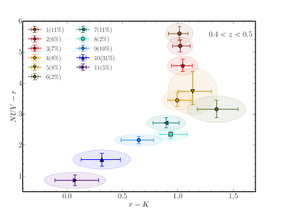
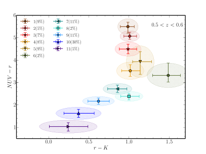
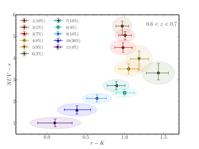
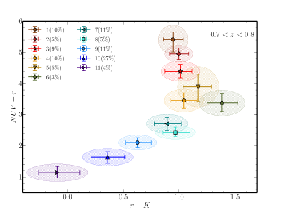
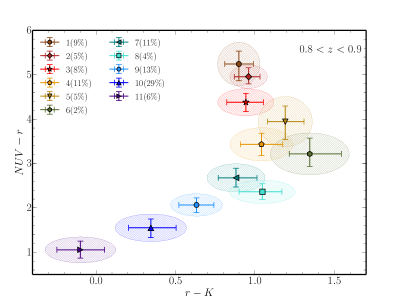
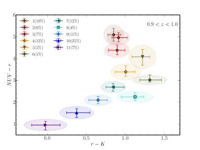
Figure 3: $NUVrK$ diagrams of the 11 FEM classes in six different redshift bins spanning the redshift range $0.4<z<1.0$. The error bars correspond to the first and the third quartiles of the galaxy colour distribution, while the two axes of the ellipses correspond to the median absolute deviations. The fraction of galaxies in each class is given in the legend.

4.2 Global properties of FEM classes

A visible separation of 11 classes in the 3D and 2D colour-colour diagrams may be expected, as the FEM classification is based on the normalised absolute magnitudes and, therefore, colours. In this section, we examine properties that were not included in the parameter space used for the automatic classification. Below we investigate morphological, spectral, mass, and star formation properties of the different FEM classes to examine whether or not there is a correspondence between our classification and these properties.

The distributions of main properties along the 11 FEM classes are shown in Figs. 5 and 6, and summarised in Table 1. In particular, the following features were derived for VIPERS galaxies: Sérsic index ($n$; calculated for VIPERS sample by Krywult et al. 2017), equivalent widths of $[OII]\lambda 3727$, the strength of the $4000\AA$ break ($D4000_{n}$, as defined by Balogh et al. 1999), and physical properties derived from SED fitting: stellar masses, and $sSFR$ (calculated by Moutard et al. 2016b). The following analysis is based on the median values of these parameters derived for each class. The error bars correspond to the first and third quartiles of the galaxy property distribution.

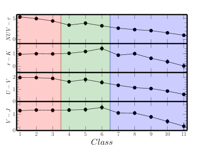
Figure 4: Colours: $NUV-r$, $r-K$, $U-V$ of the 11 FEM classes as a function of class number. The median values of parameters for red (classes 1–3), green (classes 4–6), and blue (classes 7–11) galaxies are shown in red, green, and blue areas, respectively.

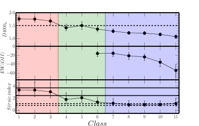
Figure 5: Spectral and morphological properties of the 11 FEM classes: $D4000_{n}$, $EW([OII]\lambda 3727)$, and Sérsic index as a function of class number. The division between red passive and blue active based on $D4000_{n}$ according to Kauffmann et al. (2003) is marked with a black dashed line. The range of mean values of Sérsic index for VIPER red passive and blue star-forming galaxies obtained by Krywult et al. (2017) are marked with black solid and dashed lines, respectively. The $[OII]\lambda 3727$ line has not been detected in the majority of galaxies within classes 1–5 (for 96, 91, 85, 59, and 72 $\%$, respectively).

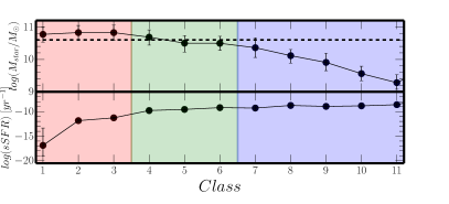
Figure 6: SED-dependent properties of the 11 FEM classes: stellar mass ($log(M_{star}/M_{\odot})$), and $log(sSFR)$ $[yr^{-}1]$ as a function of class number. The transition mass found for VIPERS galaxies at $z\sim 0.7$ by Davidzon et al. (2013) is shown with a dashed line.

To trace the change of spectral properties along the FEM classes, the strength of the $4000\AA$ break and equivalent width of $[OII]\lambda$3727 of individual galaxies in each FEM class is measured. Figure 5 shows the weakening of the median $4000\AA$ break, and the increasing of the median EW($[OII]\lambda$3727) with increasing class number. Galaxies within classes 1–3 have $D4000_{n}$ greater than 1.5 (dashed line in Fig. 5), and simultaneously display negligible emission in $[OII]\lambda$3727, while galaxies within classes 7–11 have strong emission in the $[OII]\lambda$3727 line, and a $4000\AA$ break lower than 1.5. The threshold for $D4000_{n}$ at 1.5, dividing actively star-forming and passive galaxy populations, has been found by Kauffmann et al. (2003) for local Universe and extended to higher redshift by Vergani et al. (2008). This cut allows us to associate galaxies hosting old stellar populations with no sign of star formation activity to classes 1–3, and younger objects with stronger on-going star formation to classes 7–11. The more detailed description of the spectral properties of the 11 FEM classes is presented in Sect. 4.4.

The reflection of our classification on different galaxy properties indicates the robustness of our approach and the fact that the proposed classification may be able to trace the evolutionary stages from blue and active to red passive types.

4.2.1 Morphological properties

One way to define the type of a galaxy is to analyse its structure. In the local Universe, passive galaxies are usually spheroidal, while star-forming galaxies are irregular or disk shaped (e.g. Bell et al. 2012). Krywult et al. (2017) showed that this is also the case for the whole mass distribution ($8\lesssim log(M_{star}/M_{\odot})\lesssim 12$) and redshift range ($0.4\lesssim z\lesssim 1.3$) of VIPERS galaxies. To describe the shapes of the light profiles of VIPERS galaxies, the Sérsic index is used ($n$, Sérsic 1963). The index has low values ($n\sim 1$) for spiral galaxies whose disks have surface brightnesses with a shallow inner profile, and high values ($n\sim 3-4$) for elliptical galaxies which have surface brightnesses with a steep inner profile (e.g. Simard et al. 2011; Bell et al. 2012; Krywult et al. 2017).

Krywult et al. (2017) showed that VIPERS disk-shaped galaxies have Sérsic index mean values in the range $n\sim 0.81-1.11$, whereas spheroid galaxies are characterised with average Sérsic indices in the range $n\sim 2.42-3.69$. As shown in the lower right panel of Fig. 5, there is a very good correlation between the FEM galaxy class and Sérsic index. FEM red passive galaxies (classes 1–3) have a median Sérsic index $n>3$, indicating a spheroidal shape, while classes 7–11 show a significantly lower median Sérsic index $n\lesssim 1$, typical for disk galaxies. For intermediate classes, the median Sérsic index is $n\sim 1.7$, confirming that classes 4–6 are mainly composed of intermediate galaxies also in terms of this structure. Krywult et al. (2017) demonstrated the strong correlation between morphology and galaxy colour, which is also reflected in our studies.

4.2.2 Physical properties

The top panel of Fig. 6 shows the median stellar masses obtained for the 11 FEM groups. The stellar mass decreases with class number. Galaxies assigned to classes 7–11 are less massive (with median stellar mass $\sim 10^{9.7\pm 0.3}M_{\odot}$) than galaxies within classes 1–3 (median stellar mass $\sim 10^{10.8\pm 0.2}M_{\odot}$). The stellar mass change is much more rapid for star-forming classes (0.3 dex per class), whereas for red passive classes the median stellar mass is almost constant (0.05 dex). Our classification follows well the location of passive and active galaxy types with respect to the transition mass. The transition mass separates blue star-forming and red passive populations, since above the transition mass, red passive galaxies dominate, and below that mass, star-forming galaxies are the most numerous population (e.g. Kauffmann et al. 2003; Vergani et al. 2008; Pannella et al. 2009; Davidzon et al. 2013). Based on the VIPERS dataset, Davidzon et al. (2013) determined the transition mass to be $log(M_{star}/M_{\odot})=10.6$ for galaxies at $z\sim 0.7$. Our classification is consistent with this result. Median stellar masses of galaxies within classes 1–3 are above the transition mass (marked with the dashed black line in Fig. 6), while classes 7–11 are located below the transition mass consistent with the fact that these galaxies are still forming stars. The intermediate galaxies within class 4 have the median stellar mass which matches the transition mass perfectly. This confirms that this is the group of sources that are just entering the passive evolutionary path. Classes 5–7 have stellar masses just below the transition mass ($10^{10.5}$ $M_{\odot}$) between the red and blue populations.

Finally, the bottom panel of Fig. 6 shows the change of $sSFR$ as a function of class number. The FEM classes are well separated in $sSFR$, with red passive galaxies (classes 1–3) showing the lowest star formation activity, whereas sources from the blue classes (7–11) have the highest sSFRs. At the same time, from Fig. 5 we can see that classes 7–11 have high $EW([OII]\lambda 3727)$, which is typical for blue star-forming galaxies (e.g. Cimatti et al. 2002). The $sSFR$ obtained for the intermediate galaxies ($log(sSFR)\sim-9$ $[yr^{-1}]$) is in agreement with the results derived for 1,745 CANDELS transition galaxies observed at $0.5<z<1.0$ ($log(sSFR)\sim-9$, Pandya et al. 2017). Summarising, the distributions of the physical properties (see Figs. 4, 5, and 6, and Table 1) show the trends of global and systematic changes along the FEM classes. The main spectral, morphological and physical properties correlate well within and among the groups, that is, the most massive spheroidal galaxies populated by old stellar populations are the reddest in comparison to the disk-shaped bluer galaxies hosting younger stellar contents. This demonstrates that our classification traces the evolutionary phases and galaxy types.

4.3 The $SFR-M_{*}$ relation

Galaxies show a correlation between their $SFR$ and stellar mass at redshifts at least up to $z\sim 6$ (e.g. Brinchmann et al. 2004; Noeske et al. 2007; Whitaker et al. 2012; Speagle et al. 2014; Salmon et al. 2015). This correlation, often called the galaxy main sequence (MS), is likely connected with the physical mechanisms responsible for galaxy growth, regulated by the accretion of gas from cosmic web and gas feedback (e.g. Bouché et al. 2010).

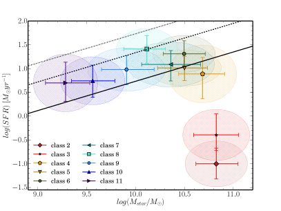
Figure 7: $SFR$–stellar mass relation for FEM classification. The median $log(SFR)$ vs. median $log(M_{star}/M_{\odot})$ for classes 2–11 are shown. The error bars correspond to the first and third quartile of the galaxy $SFR$-stellar mass distribution, while the area of ellipses correspond to the median absolute deviations. The colours are given as in Fig. 2. The first class is not plotted due to its very low median $SFR$. The black solid line corresponds to the MS trend at $z=0.7$ found by Whitaker et al. (2012), while dashed and dashed-dotted lines correspond to $4\times MS$, and $10\times MS$ to represent active star-forming and starburst galaxies, respectively, following Rodighiero et al. (2011).

The $SFR$ dependence on stellar mass for the different FEM classes is shown in Fig. 7. The black solid line corresponds to the MS at $z=0.7$ according to Whitaker et al. (2012). Whitaker et al. (2012) have established the slope and the normalisation of the $SFR(M_{*})$ as a function of redshift allowing us to reproduce the MS trend at $z=0.7$, the median redshift of VIPERS galaxies. Passive galaxies within classes 2–3 (class 1 is not presented in Fig. 7 due to its very low SFR; $log(SFR)=-6.1$ $[M_{\odot}yr^{-1}]$) occupy an area well below the MS line. The star-forming galaxies assigned to classes 7–11 instead follow the tight MS trend, showing a steady increase in $SFR$ with stellar mass as expected for the MS at this redshift. Therefore, this confirms classes 7–11 to be representative clusters of star-forming MS galaxies. However, we note that most of these median values are above the solid line. The global offset for star-forming galaxies could be due to the extinction law and SFH used for SED fitting. The Calzetti et al. (2000) extinction law is characterised by larger attenuations at longer wavelengths which results in lower stellar masses compared to other recipes such as Charlot & Fall (2000) or Lo Faro et al. 2017 (for more detailed discussions we refer to Lo Faro et al. 2017 and Małek et al. in prep.). Therefore, we relate the offset in the $SFR$ to the method used to calculate $SFR$. Whitaker et al. (2012) used the Kennicutt (1998) relation which assumes a constant $SFR$. This assumption leads to the overestimation of the $SFR$ with respect to the other SFHs in the literature (and with respect to the delayed SFH used for the SED fitting; e.g. Lo Faro et al. 2017). To summarise, the different models used for VIPERS SED fitting and to obtain the MS relation have influence on the observed offset in Fig. 7. Galaxies assigned to class 8 show a $SFR-M_{*}$ relation slightly above MS. However, we stress that within uncertainties this class is still consistent with the trend defined by the other classes. The median $SFR$ of galaxies in class 8 is located at $4\times MS$ (dashed line), which is attributed to galaxies with enhanced star formation (Rodighiero et al. 2011). This class is also characterised by redder $r-K$ colours than, for example, class 7, and a strong $H_{\beta}$ line, but not one stronger than the $H_{\beta}$ line for class 10 (see Fig. 9).

4.4 Spectral properties

In this section, the spectral properties of the photometrically motivated classes are presented. To compare the spectral properties to the classification scheme, the stacked spectra for each of the 11 FEM classes were derived. The spectra were co-added in narrow redshift bins ($\delta z=0.1$ from 0.4 to 1.0) in the same way as described in Siudek et al. (2017). Firstly, the rest-frame spectra were re-sampled to a common wavelength grid. Individual spectra were normalised by dividing the flux at all wavelengths by the scaling factor derived using median flux computed in the wavelength region $4010<\lambda(\AA)<4600$. The stacked spectra were then obtained by computing the mean flux from all individual spectra at all wavelengths in the common wavelength grid, and rescaled by multiplying the flux at all wavelengths by an average value of scaling factors of the individual spectra. Given the large sample of VIPERS galaxies, the constructed stacked spectra are characterised by a signal-to-noise ratio (S/N) high enough to detect absorption lines that are undetectable on typical, individual spectra (e.g. the $H\delta$ line; see details in Siudek et al. 2017).

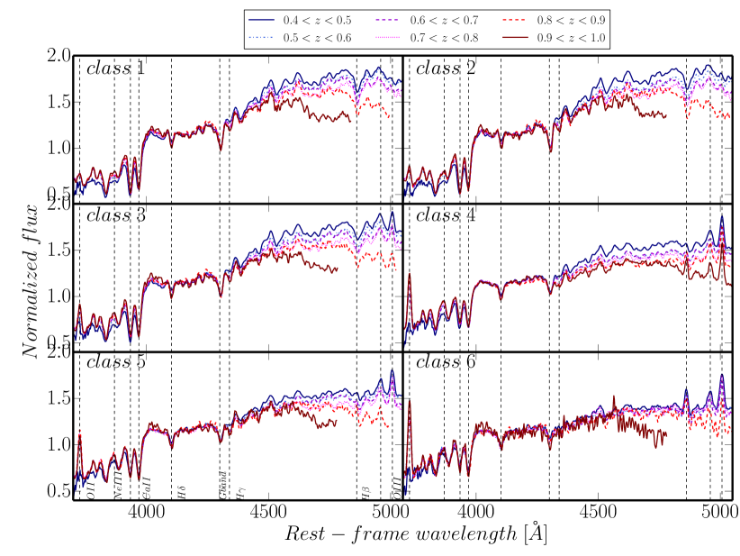
Figure 8: Stacked spectra of VIPERS galaxies among FEM classes 1–6 in different redshift bins. Rest-frame composite spectra were normalised in the region $3600<\lambda<4500$ $\AA$. The most prominent spectral lines are marked with vertical solid lines with labels.

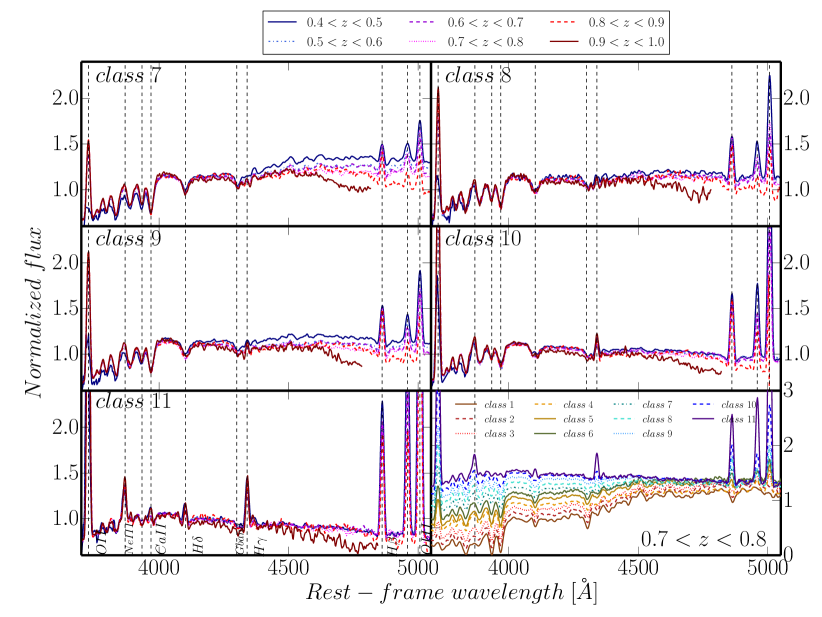
Figure 9: Stacked spectra of VIPERS galaxies among FEM classes 7–11 in different redshift bins. Rest-frame composite spectra were normalised in the region $3600<\lambda<4500$ $\AA$. The most prominent spectral lines are marked with vertical solid lines with labels. The last panel shows stacked spectra of FEM classes 1–11 in redshift bin $0.7<z<0.8$.

Figures 8 and  9 show the stacked spectra of the 11 FEM classes in six redshift bins spanning the redshift range $0.4<z<1.0$. The stacked spectra show that there is a gradual change as a function of class number. The lines go from absorption (in the first class) to strong emission (in the eleventh class).

All composite spectra of galaxies assigned to classes 1–3 are dominated by absorption lines and show weak emission lines. We can clearly see the strong $4000\AA$ break, G-band $(4304\AA)$, and Balmer lines over most of the redshift range, even if some of these features are not observed at $z>0.8$ because of the wavelength range $5500-9500\AA$ of VIPERS spectra; see  Scodeggio et al. (2018) for details. The strong absorption lines for these features are typical for early-type galaxies (e.g. Worthey et al. 1994; Worthey & Ottaviani 1997; Gallazzi et al. 2014; Siudek et al. 2017). Therefore, we conclude that the spectral properties indicate that galaxies in classes 1–3 consist of old stellar populations. From Fig. 8, we can see that the $H\delta$ line is getting stronger with redshift for all three red passive galaxy classes, which may be simply indicating that stellar populations are getting older as time passes. There is also a change in the relative strength of the CaII H ($3969\AA$) and CaII K ($3934\AA$) lines, as the CaII K line dominates at $z\sim 1$, while the CaII H line dominates at lower redshifts, especially for galaxies in class 3. The CaII K line dominates in galaxies with old stellar populations, whereas CaII H dominates when the younger stars appear.

Spectra of the green group (classes 4–6) show properties in-between the red and blue populations (see also Vergani et al. 2017). The representative stacked spectra of classes 4 and 5 are characterised by strong emission in the $[OIII]\lambda\lambda 4959,5007$ doublet with no or little sign of the recombination line $H\beta$ at redshift range $0.4<z<0.7$. Since a high ratio of $[OIII]\lambda\lambda 4959,5007$ to $H\beta$ lines is an indication of AGN photo-ionisation, this suggests that a non-negligible fraction of galaxies in these classes may host a Seyfert nucleus. However, this is not confirmed by the localisation of classes 4 and 5 on the BPT diagram (see Sect. 4.4.3), even if only galaxies within redshift range $0.4<z<0.7$ are considered. Therefore, we are not able to conclude whether those galaxies host a Seyfert nucleus or not. The stacked spectra of intermediate galaxies within class 6 show diagnostic lines (e.g. $[OII]\lambda 3727$, $[NeIII]\lambda 3869$, $H\beta$) in emission. There is also a hint of star formation activity in the intermediate classes (4–6) revealed by detectable emission in the $[NeIII]\lambda 3869$ line in all redshift ranges (Ho & Keto 2007).

The stacked spectra of galaxies in classes 7–11 show that they are undergoing a significant level of star formation, indicated by prominent emission lines, like the $[OII]\lambda 3727$ or $H\beta$ lines, and a weak $4000\AA$ break (e.g. Mignoli et al. 2009; Haines et al. 2017). The emission lines are getting stronger with increasing class number of star-forming galaxies. The possibility of AGNs is further discussed in Sect. 4.4.3. In this paper, we focus on general properties of the whole classification scheme. The detailed properties and evolutionary trends of the FEM classes will be discussed in future papers.

4.4.1 The comparison of FEM classes with Kennicutt’s Atlas

To better define the morphological and spectral types of each of the 11 FEM classes, we compare their representative stacked spectra with those of galaxies of different Hubble types as given by Kennicutt (1992). Kennicutt’s Atlas consists of 55 integrated spectra of nearby galaxies, covering the wavelength range $3650<\lambda[\AA]<7100$ with a resolution of $5-8\AA$, grouped according to their morphological and spectral types.  Kennicutt (1992) provides a set of individual normal and peculiar galaxies following the Hubble sequence, from giant ellipticals ($NGC1275$) to dwarf irregulars ($Mrk$35). We compared the 11 FEM classes with the Atlas by assigning to each FEM class the best spectrum in the Atlas based on the $\chi^{2}$ minimisation. The 11 FEM classes tend to follow the Hubble sequence as classes 1–3 show morphologically earlier types than the other classes. Stacked spectra of galaxies in classes 7–11 are quite well reproduced by the spiral, irregular, and emission-line galaxies (Sc, Im), whereas spectra of Sb galaxies best fit the stacked spectra of intermediate galaxies (classes 4–6), and the template spectrum of Sab galaxy fits the representative stacked spectra of classes 1–3. The detailed comparison of spectral properties of the 11 FEM classes to the spectral Atlas of Kennicutt (1992) is discussed in Appendix D.

4.4.2 Comparison to principal component analysis (PCA) classification of VIPERS galaxies

In this section, we compare the FEM classification to a classification scheme used within the VIPERS survey by Marchetti et al. (2013), based on the PCA technique applied to spectra of VIPERS galaxies. The PCA-based algorithm divided VIPERS galaxies into 15 different clusters based on the first three eigen coefficients ($\theta-\phi$ diagram). The PCA classification distinguished eight groups among the red and intermediate galaxy types from E to Sc, and seven classes of more active starburst galaxies. We find that our classification follows the track found by Marchetti et al. (2013), since the reddest, early-type galaxies fall in the region of the bottom left edge of the $\phi-\theta$ diagram, and with increasing $\theta$ and $\phi,$ the number of the FEM class is increasing, which implies that galaxies are bluer (see Fig. 15).

We find that $\sim 70\%$ of early-type galaxies selected with PCA (PCA classes 1–2 contain E and Sa galaxies) are distributed in the FEM classes 1–3. This indicates the similarities in the capability of separation of ETGs, especially the oldest ones, in the VIPERS dataset by both methods. The dusty spiral galaxies, $\rm{Sb_{4,6}}$ (with $E(B-V)>0.4$; Kinney et al. 1996), assigned to PCA classes 3–6 are spread among various FEM classes, with the majority of them ($\sim 70\%$) being located in the FEM classes 7–11. Almost all Sc galaxies ($\sim 95\%$) selected by PCA (PCA classes 7-8) are assigned to the FEM classes 9-11. The spiral galaxies with smaller amounts of dust, $\rm{Sb_{1,2}}$ (with $E(B-V)<0.2$; Kinney et al. 1996), within PCA classes 9–13, are also found among FEM classes 10–11 ($\sim 80\%$ of them).

This shows that there is a global agreement between the FEM and PCA classification schemes. However, it should be noted that these two classification schemes, being based on different input data (photometric data for FEM, and spectroscopic for PCA), are not fully coherent with each other and therefore do not show precisely the same patterns. In Appendix C it is shown how well, using the derived eigenvalues for VIPERS PDR1, the FEM classes are separated in the $\theta-\phi$ PCA diagram.

4.4.3 The Baldwin, Phillips & Terlevich diagram

To differentiate star-forming galaxies from AGNs, we checked the distributions of the intermediate and star-forming galaxies (classes 4–11) on the diagnostic diagram for emission-line galaxies. The distribution of VIPERS galaxies in the BPT (Baldwin et al. 1981) diagram is shown in Fig. 10. We are able to separate LINERS and Seyferts based on their emission line ratios. We measured emission lines on individual spectra within the redshift range $0.4<z<1.3$ assigned to classes 4–11, and the $H\beta$ measurements were corrected for an average absorption component. The distribution of VIPERS galaxies assigned to classes 4–10 indicates that those galaxies are star-forming galaxies. Class 11 is placed in the composite area (SF/Sy2 in Fig. 10), which may indicate that it contains AGNs. The contamination by broad-line AGNs has no influence on our result, as only line measurements of galaxies within redshift range $0.4<z<1.0$ and redshift flag 3–4 are included (i.e. excluding the flags corresponding to broad-line AGN). However, AGNs are very rare among low-mass galaxies (the median stellar mass of galaxies within class 11 is $\sim 10^{9}$ $M_{\odot}$), therefore, we suspect that these might be low-metallicity galaxies. However, both these options (AGN contributions and low-metallicity galaxies) are consistent with the spectroscopic properties of this group (see Sect. 4.4), as the spectra show strong emission lines.

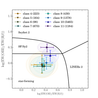
Figure 10: The distributions of FEM classes 4–11 on the ”blue” BPT diagram introduced by Lamareille (2010). The number of spectra in each class for which lines were measured in the redshift range $0.4<z<1.3$ are given in the legend. The error bars correspond to the first and third quartile of the line measurements distribution, while the area of ellipses correspond to the median absolute deviations.

5 Summary

In this paper, a new approach to galaxy classification is introduced, based on the thirteen-dimensional parameter space built from 12 absolute magnitudes and the spectroscopic redshift. An unsupervised classifier based on the FEM algorithm blindly separated 52,114 VIPERS galaxies into 12 classes. The model selection (DBk) and the determination of the optimal number of classes were based on statistical criteria (BIC, AIC and ICL; see Appendix B) and found to be in the range 9–12. Subsequently, the final class number (12) was decided based on the analysis of the galaxy flow with a changing number of groups (see Fig. 12), and the interpretation of physical properties of classes in different realisations (see Fig. 1). All these techniques resulted in the same model and an optimal number of 12 classes in the VIPERS dataset. These classes follow a well-defined sequence from the earliest to the latest types, separating galaxies into three major groups: red, green, and blue. The FEM classification automatically finds groups that share physical and spectral properties, beyond the features used for classification purposes. Galaxies are not unequivocally assigned to a single class, but the probability of belonging to each group is given. Such an approach is more realistic as the transition between classes can be continuous. In spite of this, a majority of galaxies ($92\%$) in the sample have high ($>50\%$, with $<45\%$ second best probability) probabilities of belonging to the selected group. We obtain three main classes: red, green, and blue, which can be further separated into subclasses: three red, three green, and five blue, and an additional class 12, which consists of outliers. For class 12, $95\%$ of its members are broad-line AGNs according to the visual classifications by the VIPERS team (Garilli et al. 2014). Their median redshift is $z_{med}\sim 2$, which removes this class from the global picture of VIPERS galaxy types observed up to $z\sim 1$.

We demonstrated that our approach leads to a new classification scheme allowing us to track galaxy evolutionary paths. The main advantage of this approach is the ability to distinguish 11 galaxy types, which share physical and spectral properties not used in the classification procedure. The presented separation between different galaxy types differs from traditional selection methods based mainly on the bimodal distribution in colours (e.g. Bell et al. 2004; Balogh et al. 2004b; Franzetti et al. 2007), spectral properties (e.g., H$\alpha$ (Balogh et al. 2004a)), $[OII]\lambda 3727$ emission (Mignoli et al. 2009), 4000$\AA{}$ break (Kauffmann et al. 2003; Vergani et al. 2008), and SFH (Brinchmann et al. 2004).

Our main results are as follows:

We present a new unsupervised approach to galaxy classification based on the multidimensional space of absolute magnitudes and the spectroscopic redshift, which does not introduce any a priori defined cuts.

We find three red, three green, and five blue classes which are distributed along a well-defined path in multidimensional space.

The borders between classes are not sharp; the probability of belonging to a given class is associated to each galaxy. However, the probabilities of belonging to a given class are high ($\sim 80\%$) and, in spite of the presence of outliers, the classes are well separated in the feature space and are therefore more faithfully representative of the full complexity of the galaxy population at these redshifts.

We show the evolution of the 11 classes over the redshift range $0.4<z<1.0$.

We demonstrate that there are significant differences in physical and spectral properties between galaxies classified as red/green/blue FEM classes and their subclasses.

We find a very good correlation between the FEM classes and spectroscopic classes in the Atlas of Kennicutt (1992). The 11 FEM groups follow the path from the earliest to the latest galaxy types.

In particular, the following FEM class properties were found:

Classes 1–3 host the reddest spheroidal-shape galaxies showing no sign of star formation activity and dominated by old stellar populations (as testified by their strong $4000\AA$ breaks).

Classes 4–6 host intermediate galaxies whose physical properties, such as colours, sSFR, stellar masses, and shapes, are intermediate relative to red, passive, and blue, active galaxies. These intermediate galaxies have more concentrated light profiles and lower gas contents than star-forming galaxies (as indicated by the Sérsic index, and $EW(OII)$). This tendency is also observed for intermediate galaxies observed in the local Universe (Schiminovich et al. 2007; Schawinski et al. 2014).

Classes 7–11 contain the star-forming galaxies. The blue cloud of disk-shaped galaxies is actively forming new stars and are populated by young stellar populations (as indicated by the weak $4000\AA$ break). Class 11 may consist of low-metallicity galaxies, or AGNs according to its localisation on the BPT diagram.

Automatic unsupervised classifications are becoming an invaluable tool in the current era of information deluge. The FEM algorithm can also be applied to photometric samples with comparable efficiency in distinguishing a full panoply of galaxy types (Siudek et al. 2018). With the increasing number of deep surveys, such as Euclid and LSST, such algorithms may allow us to study galaxy formation and evolution across the lifetime of the Universe. The presented classification scheme has great potential, as we can ascertain the class to which a galaxy or a galaxy region belongs. Based on defined classes, different stellar populations can be traced and galaxies within structures can be classified.

Appendix A Determination and validation of the number of classes

The AIC, BIC, and ICL are standard criteria widely used in machine learning algorithms to evaluate the statistical model.

• AIC - The Akaike information criterion penalises the log-likelihood by $\gamma(M)$, where $M$ is the used model and $\gamma$ is the number of parameters in this model (Akaike 1974). The AIC is used to select the best model from the available pool. Using this criterion, we search for the model closest to reality with a minimum number of parameters. It was first introduced to cosmology by Takeuchi (2000).

• BIC - The Bayesian information criterion is the most popular criterion which penalises likelihood by $\frac{\gamma(M)}{2}log(n)$, where $M$ is the used model and $n$ is the number of observations (Schwarz 1978). BIC is analogous to AIC (Bouveyron & Brunet 2011), but is derived from Bayesian statistics.

• ICL - The integrated complete likelihood penalises the log-likelihood by $\sum^{n}_{i=1}\sum^{K}_{k=1}t_{ik}\log(t_{ik})$ in order to favour well-separated models, where $k$ is the number of mixture components, $i$ is the number of observables, and $t$ is the posterior probability (Baudry 2012).

In this paper, all three criteria are applied. They allow us to compare different DLM models and define the optimal number of groups in the data. The AIC and BIC are widely used penalised likelihood criteria, while ICL is an alternative approach, which starts with the BIC criterion and adds a so-called entropy component (the sum of posterior probability memberships given by $\sum_{i}\sum_{j}pp_{ij}ln(pp_{ij})$, where $pp_{ij}$ is the $i$’s posterior probability membership in $j$-group). Therefore, the scoring between AIC/BIC cannot be directly compared to ICL scoring.

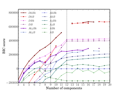
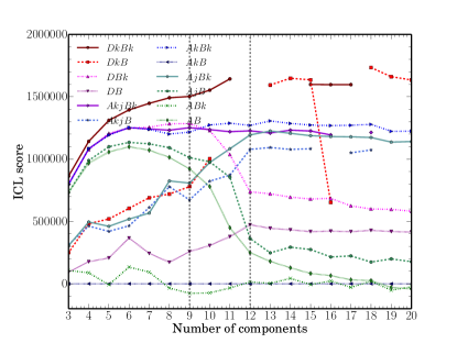
Figure 11: Results of model and number of classes chosen based on the BIC and ICL criterion. Number of components corresponds to number of classes.

Each criterion (AIC, BIC and ICL) consists of two parts: the former increases the score for models with increasingly well separated groups, and the other is responsible for penalising an excessive number of groups. Otherwise, the division which receives the highest score would be the one in which every object was a separate group (Bouveyron & Brunet 2011). Based on the received scores the optimal number of groups can be chosen.

The change of BIC (AIC is not shown as it mostly gives the same scoring as the BIC criterion) and ICL scoring for different numbers of classes and models is shown in Fig. 11. The algorithms were unable to converge (and therefore unable to calculate the scoring) for some combinations of numbers of classes and models, resulting in discontinuities in the DkBk and DkB curves. Although the DkB and DkBk models have higher AIC/BIC scores, we did not decide to use them. The DkBk model is unstable for more than 11 components, where it is expected to achieve a maximum (i.e. the most preferable number of classes) and therefore the optimum number of classes cannot be specified. The similar situation is observed for the DkB model, which is unstable for steps 11 and 12 and for this reason it is impossible to state its behaviour and find the maximum. Based on Fig. 11 we can see that the AIC/BIC scores for the DBk and DB models are very similar. However, when we consider the ICL scores, we see significant differences in favour of the DBk model. Therefore, we decided to use the DBk model which gives the best scoring among all the three criteria. For a detailed description of the DBk model see Bouveyron & Brunet 2011. According to Fig. 11, the BIC scores increase steadily as the number of classes is increased, up to a limit of 12 classes. The scores do not continue to increase for models with more than 12 classes, and so we consider 12 classes to be the optimal choice. The ICL criterion achieves its maximum score for nine classes. The ICL scores decrease rapidly from step 9 to step 10, and declines further to 12 classes. Above this number, the model score (as in case the of BIC criterion) practically does not change. Based on the analysis of the BIC, AIC, and ICL criteria, we conclude that the optimum model is the DBk model with approximately nine (according to the ICL criterion) or twelve (according to the AIC and BIC criteria) classes.

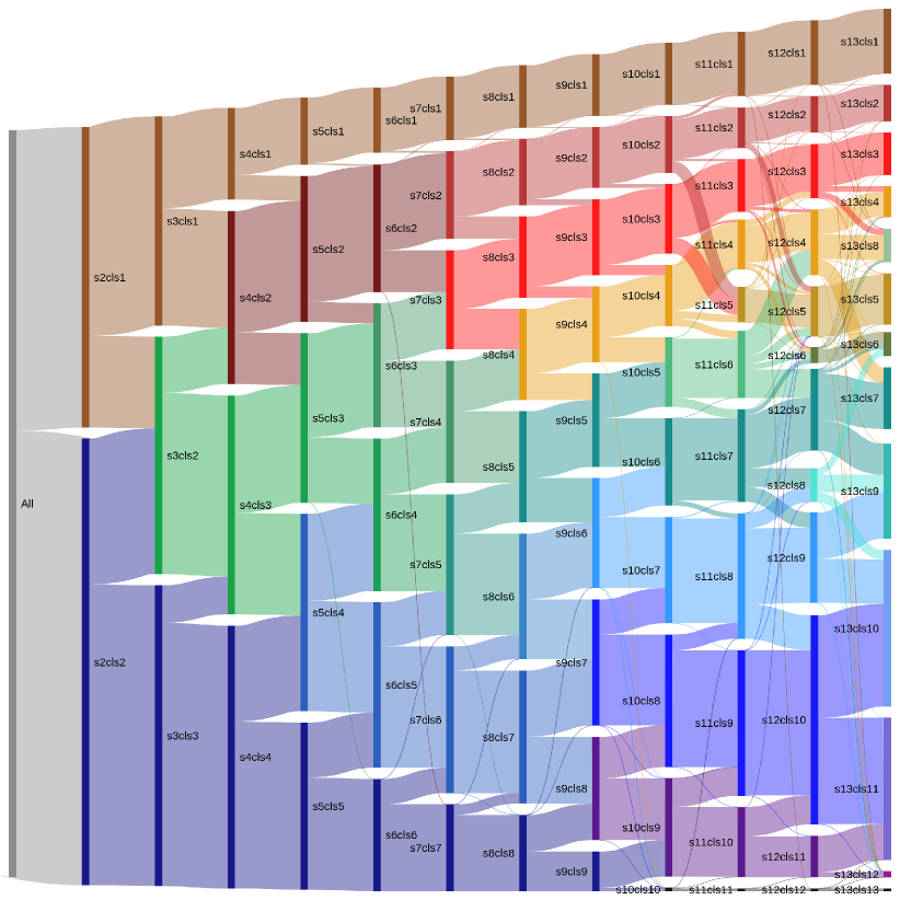
Figure 12: The dependence of galaxy distribution on the number of classification steps. The galaxy flow beginning from one single class up to the classification with thirteen classes is shown. The step number (equal to the number of classes) followed by the class number is given (s2cls1, where s2 corresponds to the second step, division into two classes, while cls1 corresponds to the first class).

In Fig. 12 we present the flow chart of 52,114 VIPERS galaxies. This includes those objects with low probabilities of being members of any class, which are less than 1% of our sample at the first step and less than 10% of our sample at the twelfth step). These are visible as thin lines that correspond to several dozen objects, which in all cases are a small percentage (3%) of all galaxies in a given group. In order to select the optimal number of classes, the galaxy flow between classifications was checked at each step, from one single class up to thirteen classes. Each step corresponds to the number of classes into which the VIPERS galaxies were classified (i.e. notation s2 corresponds to the second step and division into two classes). Figure 12 shows that some classes (e.g. cls1, where 1 corresponds to the first class) are well separated in the very early steps (cls1 is basically unchanged for s4–13), while others (e.g. s12cls7) are formed from a mixture of galaxies from different classes from the previous steps. This is also mirrored by their posterior membership probabilities, as well-defined classes (e.g. s12cls1) have high membership probabilities, while ”flowing” classes (e.g. s12cls7) are characterised by lower probabilities. The new classes distinguished between steps 10 and 12 (12cls6, 12cls8, 12cls12) are characterised by relatively small numbers of galaxies (see Fig. 14) and tend to separate beside the main linear trend formed by s9cls1-s9cls9 (see the first panel in Fig. 1). In particular, class 12cls12 is separated in step 10 (s10cls10), while in steps 11 and 12 the classes containing dusty star-forming galaxies (s12cls5, s12cls6, and s12cls8) are distinguished. Based on the physical properties of these newly separated classes in s11-12 (see Fig. 1), we found each of them to be representative of distinct galaxy types, and therefore, we found 12 classes as the optimal number of galaxy types reflecting a full panoply of VIPERS dataset. We also verified that forcing the algorithm to separate one more additional group (step 13) does not lead to formation of a well-defined (with respect to physical galaxy properties, see Fig. 13) new class (s13cls12), which emerges from 12cls11, however do not reveal distinct properties at least in its colours.

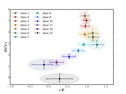
Figure 13: $NUVrK$ diagrams of FEM classes 1–13. The error bars correspond to the first and the third quartile of the galaxy colour distribution, while the two half axes of the ellipses correspond to the median absolute deviation

A detailed description of the diagram  12 will be discussed in Krakowski et al. in prep.

Appendix B Class membership probabilities

The FEM algorithm assigns each VIPERS galaxy to one of the 12 classes. However, the classification does not provide sharp borders between classes. The class membership probability is based on the distance of an object from the centre of the class in the multidimensional feature space. Therefore, each galaxy is characterised by the posterior probability of it belonging to a particular class. This has allowed us to quantify the number of galaxies with problematic classifications that could belong to two or more classes with roughly similar probabilities.

In our case, the classes found by the FEM algorithm are well defined, as the majority of their members are well separated from the neighbouring classes. This is reflected by the majority of galaxies having a high probability of being a member of the class to which they are assigned. Therefore, almost all galaxies ($94\%$) have high probabilities ($>50\%$) of belonging to their assigned class. The remaining $6\%$ are outliers, which do not fall into any class.

Among the $94\%$ of ”well classified” galaxies (with $>50\%$ probability of class membership) $2\%$ also have $>45\%$ probability of belonging to the second-best class, implying that those galaxies are midway between two classes. Although the numbers of sources at the borders of the classes (1,038) and other outliers (2,947) is very small (in total $8\%$ of the sample), we exclude them from the final set used to analyse properties of the FEM classes.

The distributions of class membership probabilities for each class are presented in Fig. 14 (marked with dark blue). The probability distribution for the final sample, including only objects with a high first-best probability ($>50\%$) and a low second-best probability ($<45\%$) is marked with light blue. Following Krakowski et al. (2016) and Kurcz et al. (2016), the influence of increasingly severe probability cuts on the quality of the estimated global properties of each class is checked. No significant improvement in purity or derived properties was found when adopting more severe cuts. Even for the purest sample, including only galaxies with class membership probabilities higher than $80\%$, the global properties of each class (reaching the highest deviation for colours, but not greater than 0.3$\sigma$) remain in a broad agreement with those obtained when less severe cuts are applied. As more severe cuts (with class membership probabilities higher than $80\%$) do not change our results, but reduce significantly the number of objects (to $56\%$ of the sample), in this paper, we applied less severe cuts (high first-best and low second-best class membership probabilities).

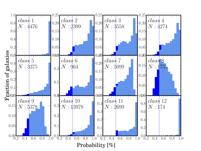
Figure 14: Distribution of the class membership probabilities for all sources (dark blue), and for the final sample of galaxies (with first-best probability $>50\%$ and second-best $<45\%$; in light blue) for each FEM class. The threshold ($50\%$) used to remove outliers in the subsequent analysis is marked with a blue dashed line. The final number of class members is given in each panel.

Appendix C Comparison of the FEM-based and PCA-based classifications of the VIPERS galaxies

To date galaxy classification has been mostly based on their colours as determined from broad-band photometry (e.g. Bell et al. 2004; Fritz et al. 2014; Siudek et al. 2017) or from their spectra (e.g. Balogh et al. 2004a; Marchetti et al. 2013; de Souza et al. 2017). One of the most common methods used to distinguish different galaxy populations from their spectra is the PCA method. In this method, each spectrum is decomposed into a set of representative templates, which reproduce the most important galaxy features (spectral slope and strong emission lines). This transformation is characterised by orthogonal vectors (eigenvectors), which describe the original spectra. Marchetti et al. (2013) have used the first three eigenvalues ($a1$, $a2$, $a3$), which have the highest importance in effectively representing the data, and provide an optimal input for spectroscopic classification. The parameter space was further reduced to Karhunen-Loéve angles ($\theta$,$\phi$; Karhunen 1947; Connolly et al. 1995). The spread of galaxies on the $\theta-\phi$ plane allows us to identify different galaxy types, as redder galaxies have smaller $\theta$, and $\phi$ values, while bluer galaxies are characterised by higher values (Marchetti et al. 2013). In order to verify how our FEM classification based on galaxy colours is relevant to spectroscopic galaxy classification we investigate the eigencoefficients for FEM classes and compare the FEM-based and the PCA-based classes.

The distribution of galaxies belonging to the different FEM classes in the $\theta-\phi$ diagram is shown in Fig. 15. The values of $\theta$ and $\phi$ were obtained by Marchetti et al. (2013), who made a classification of the spectra of the VIPERS galaxies from the PDR-1 making use of the Kinney–Calzetti templates (Calzetti et al. 1994; Kinney et al. 1996), which we also use for comparison (see the last panel in Fig. 15).

We examine the FEM classification of the PCA-based galaxy types from early types (E) at the bottom, through the star-forming (Sa and Sb) populations, and up to the Sc galaxies in the top of the diagram. Lower-$z$ red passive galaxies (classes 1–3) are tightly located in the bottom edge of the $\theta-\phi$ diagram, in the locus of the early-type family of galaxies ($\theta<1.6$ and $\phi$¡0). With increasing redshift, the galaxies of classes 1–3 tend to move to the region of Sa, almost reaching the area where the Sb6 are placed. This shows how passive galaxies evolve with cosmic time, showing a hint of star formation activity in earlier epochs and quenching with cosmic time. Green intermediate galaxies (classes 4–6) tend to have a similar distribution to sources within classes 1–3, although they show a larger scatter, especially in $\phi$, revealing extended star formation activity. This may be attributed to them being in the intermediate stage between red passive and blue star-forming galaxies. The star-forming galaxies (classes 7–11) follow a sequence on the $\theta-\phi$ diagram ending with galaxies assigned to class 11 being distributed in the top-left corner. This area is dominated by the templates of galaxies which are actively forming new stars (Sb, and Sc). This is especially significant for classes 10 and 11, since galaxies form a tail beginning in the area of Sb and Sc templates with a sharp cut in redshift.

The presented good correlations with eigenvalues show that we can use FEM classification based on rest-frame magnitudes when galaxy spectra of good quality are not available.

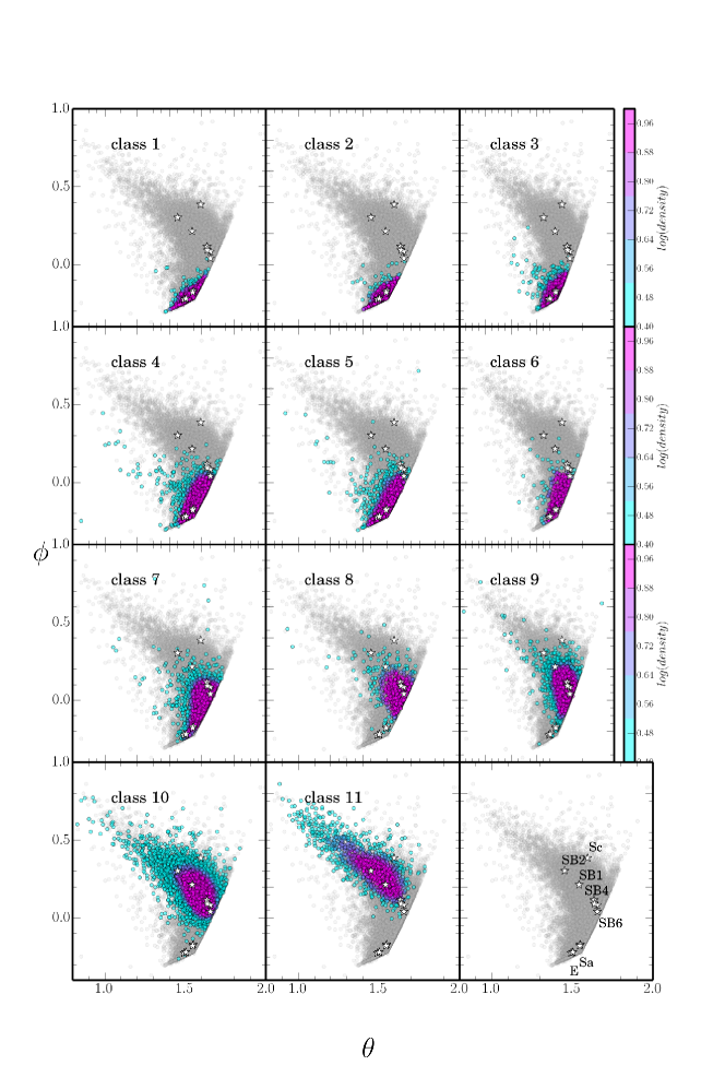
Figure 15: PCA components derived from VIPERS spectra by Marchetti et al. (2013) for the 11 FEM classes. VIPERS PDR1 galaxies are marked with grey dots. The distribution of 2688, 1428, 2185, 2674, 2201, 598, 3300, 1096, 3630, 7885, 1395 eigen coefficients for the 11 FEM classes are colour-coded according to their redshift values. The location of the Kinney–Calzetti spectra (Calzetti et al. 1994; Kinney et al. 1996) for different galaxy families are marked with white stars following Marchetti et al. (2013).

Appendix D Relation between FEM classes and Hubble types

One of the methods to classify galaxy optical spectra is to examine their structures and compare them to the Hubble sequence, or its variations. Spectral types may be derived through spectral features or SED fitting (e.g. Sánchez Almeida & Allende Prieto 2013; Conselice et al. 2011). In this paper, we adopt the approach of Sánchez Almeida & Allende Prieto (2013), and compare optical composite spectra of the 11 FEM classes with the spectral types defined in the Atlas of Kennicutt (1992). To fit the observed spectra against models, we first rest-framed the spectra, downgraded their resolution to $14\AA$ (corresponding to the typical resolution of VIPERS spectra as shown by Siudek et al. 2017), and normalised the template spectra over the wavelength range $3800<\lambda(\AA)<5500$. The observed spectra were stacked within each FEM class in redshift range $0.5<z<0.6$ and normalised in the same wavelength range as the templates. For each of the 11 representative stacked spectra we performed a $\chi^{2}$ minimisation over the entire Kennicutt Atlas. Based on the $\chi^{2}$ we determined the best template for each FEM class.

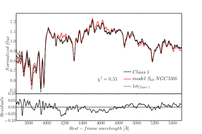
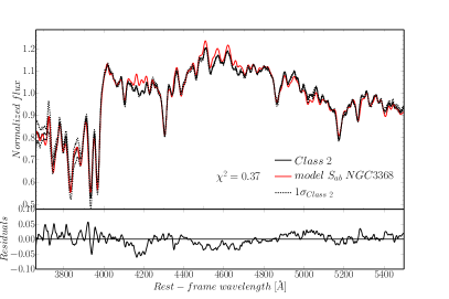
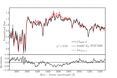
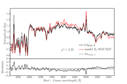
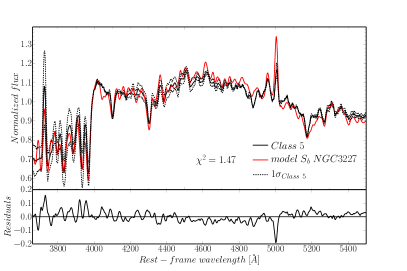
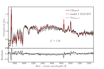
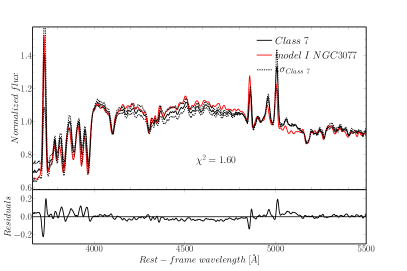
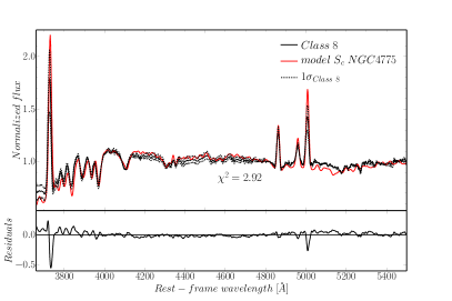
Figure 16: The comparison of the 11 FEM stacked spectra in redshift bin $0.5<z<0.6$ with the best-fit template spectra from the spectral Atlas of Kennicutt (1992).

Figures 16 and 17 show the 11 FEM representative stacked spectra of VIPERS galaxies observed in the redshift range of $0.4<z<1.3$ (marked with the black solid line). The $1\sigma$ stacked spectrum is marked with a dashed line, and the best template is over-plotted in red. Red passive galaxies (classes 1–3) show no difference with respect to their spectral type, since for each representative spectrum the best spectral template corresponds to the Sab type of $NGC$ $3368$ galaxy from the Kennicutt Atlas (see the first three panels in Fig. 16). The models fit the observed spectra remarkably well, especially the main features that can be attributed to old stellar populations, including $D4000$, $H\delta$, and $G-band$ showing no difference with respect to the template spectrum. The family of Sab galaxies is dominated by evolved giant stars, but there can also be found a contribution from younger stellar populations (Kennicutt 1992). When it comes to their visual appearance, the Sa group contains non-barred galaxies, whereas Sb is assigned to barred galaxies, and Sab refers to intermediate sources, showing weak signs of a bar (an oval one in the case of $NGC3368$ according to Kennicutt 1992). However, $NGC3368$ is also classified as unbarred Sa according to other authors (Sandage 1961; Kormendy & Kennicutt 2004). It should be noted that the VIPERS stacked spectra of red classes (1–3) are very well fitted by the templates of E galaxies (especially with E1 $NGC3379$). Among the best-fitting templates for stacked spectra of classes 1–3, types E/S0/Sa dominate. The template spectra of elliptical galaxies do not show strong differences with respect to spectra of Sab/Sa/S0 galaxies, as all of them are dominated by strong absorption lines typical for red galaxies with old stellar populations. Those templates present strong $4000\AA$ breaks and strong absorption lines (G-band, $H\delta$ line) typical for old stellar populations. The best template was assigned to Sab mainly because of the best fit to the $[OII]\lambda 3727$ line, which is not seen in absorption as in elliptical galaxies according to spectroscopic Atlas of Kennicutt (1992). However, the spectrum of this intermediate family appears to have features typical for old stellar populations (i.e. strong $4000\AA$ break and strong absorption line $[H\delta]\lambda 4102$). The stacked spectra of green galaxies assigned to class 4 and 5 are best fitted with the template of the spiral galaxy Sb $NGC3327$. The classification of $NGC3227$ galaxy is tentative, as it is classified as a peculiar object within a family of Sab sources according to de Vaucouleurs et al. (1991). Kennicutt (1992) has assigned this template as the spectrum of strongly interacting/merging galaxy with a Seyfert 2 nucleus. Although the BPT diagram (see Fig. 10) does not confirm that these galaxies are Seyfert galaxies, we do not exclude the possibility of AGNs belonging to those groups. Although the spectra do not present any broad Balmer lines indicating clearly the presence of active nuclei, the high-excitation emission-lines combined with red continuum can be interpreted as a signature of AGN (Kennicutt 1992).

The irregular galaxy $NGC3077$ template shows the best fit to the representative stacked spectrum of galaxies in classes 6 and 7. Although some of the templates of Sb and Sc families show comparable values of $\chi^{2}$, neither of them are able to fit well the $H\beta$, $[OIII]$ lines and the $4000\AA$ break at the same time. Irregular galaxies do not fall into a regular classification showing some unusual features, mainly involving peculiar asymmetries or shapes, however the spectrum of $NGC3077$ is not distinguishable from a spectrum of normal Sc galaxy based only on the spectrum (Kennicutt 1992). Interestingly, according to Buta et al. (2015), this galaxy appears as an early-type galaxy in $3.6\mu m$ images with a very scattered dust distribution. The spectrum is very similar to the spectra of the blue ”E+A” galaxies, except of the presence of the $[NII]$ and [OII] emission lines.

Stacked spectra of star-forming galaxies in classes 8 and 9 are well fitted with the spectrum of the Sc galaxy $NGC4775$. According to the morphological properties, the $NGC4775$ galaxy is classified as the late-type spiral galaxy with flocculent spiral arms (Buta et al. 2015). Spectra of the Sc family qualitatively differ from those of earlier Hubble types with respect to their continuum shape, absorption and emission features. They present strong principal emission lines, like $H\beta$, and $[OIII]$.

The stacked spectrum of galaxies assigned to class 10 is best-fit with a template spectrum of the peculiar I galaxy $UGC6697$. This family is built from star-forming galaxies with much stronger emission lines than the average strengths observed in Sb or Sc families (3-10 times higher EW($H\alpha,NII$) Kennicutt 1992). Therefore, class 10 represents galaxies which are undergoing global bursts of star formation.

The Im galaxy $MK35$ fits best the representative stacked spectrum of class 11. This template characterises an extreme emission-line galaxy, and might represent a new-born galaxy. The galaxy is filled with gas and is in the phase of the global burst of star formation.

The stacked spectrum of broad-line AGNs (class 12) is shown in the last panel in Fig. 16, but is not compared to the Atlas of Kennicutt (1992) due to a lack of broad-line AGN templates.

In conclusion, the 11 FEM classes follow the Hubble sequence according to spectroscopic types given by the Atlas of Kennicutt (1992). Classes 1–3 present spectra typical for early-type galaxies, while classes 7–11 demonstrate spectra of actively star-forming galaxies with extreme emission-line galaxies in the highest class, with green galaxies showing spectra of intermediate types.