Error-Controlled Exploration of Chemical Reaction Networks with Gaussian Processes

Abstract

For a theoretical understanding of the reactivity of complex chemical systems, relative energies of stationary points on potential energy hypersurfaces need to be calculated to high accuracy. Due to the large number of intermediates present in all but the simplest chemical processes, approximate quantum chemical methods are required that allow for fast evaluations of the relative energies but at the expense of accuracy. Despite the plethora of benchmark studies, the accuracy of a quantum chemical method is often difficult to assess. Moreover, a significant improvement of a method’s accuracy (e.g., through reparameterization or systematic model extension) is rarely possible. Here, we present a new approach that allows for the systematic, problem-oriented, and rolling improvement of quantum chemical results through the application of Gaussian processes. Due to its Bayesian nature, reliable error estimates are provided for each prediction. A reference method of high accuracy can be employed, if the uncertainty associated with a particular calculation is above a given threshold. The new data point is then added to a growing data set in order to continuously improve the model, and as a result, all subsequent predictions. Previous predictions are validated by the updated model to ensure that uncertainties remain within the given confidence bound, which we call backtracking. We demonstrate our approach at the example of a complex chemical reaction network.

1 Introduction

The accurate description of chemical processes requires elucidation of a reaction network comprising all relevant intermediates and elementary reactions. For a kinetic analysis, the thermodynamic properties of all intermediates and transition states in this network need to be determined to high accuracy. While state-of-the-art quantum chemical calculations can yield highly accurate results even for large systems,[1] they are computationally expensive and, therefore, restricted to a limited number of elementary steps. For this reason, density functional theory (DFT) remains to be the method of choice, despite its shortcomings with respect to accuracy and systematic improvability. The known existence of the exact exchange-correlation functional[2, 3] and numerical demonstration[4] of rung-by-rung accuracy of approximate functionals across Jacob’s ladder[5] have nurtured the hope to eventually arrive at approximate functionals of sufficiently high quality. However, popular hybrid density functionals struggle to reproduce experimental ligand dissociation energies of large transition-metal complexes (see, e.g., refs. [6, 7, 8, 9, 10, 11, 12, 13, 14, 15]).

The accuracy of approximate exchange–correlation density functionals is often assessed through benchmark studies. While many extensive data sets exist, such as the ones proposed by Pople,[16, 17, 18, 19] Truhlar,[20, 21, 22, 23, 24, 7, 25, 26, 27, 28] and Grimme,[29, 30, 31] studies have shown that the accuracy of density functionals can be strongly system-dependent.[18, 19, 32, 23, 33, 9, 11] Even if accurate reference data for given molecular structures were available, one could not assume the error of a DFT result to be transferable to the close vicinity of that particular region of chemical space.[34, 11, 35, 13, 36, 14] Finally, even if one had some upper bound on the error of a calculated property, this bound would be so large that subsequent analyses, such as kinetic studies, would be rendered meaningless.[37] If, however, an error estimate of each result was known, the value of any approximate DFT approach would be dramatically increased as it would flag those results to be considered with caution. An assigned uncertainty would allow one to judge whether conclusions drawn from the data are valid or not.

A few methods have been developed that aim at providing systematic error estimates for individual DFT results. In 2005, Sethna, Nørskov, Jacobsen, and co-workers presented an error estimation scheme based on Bayesian statistics [38] (see also refs.  39, 40, 41). Instead of focusing on only the best-fit parameters in a density functional, an ensemble of parameters was drawn from a conditional distribution over parameters by which a mean and a variance could be assigned to each computational result.[42, 43, 44] While the developed functionals were parametrized on a wide range of reference data sets, the issue of transferability remained. In addition, the reliability of the error estimates was limited.[45] Recently, Zabaras and co-workers[46] developed a new exchange-correlation functional to predict bulk properties of transition metals and monovalent semiconductors. Furthermore, Vlachos and co-workers successfully applied Bayesian statistics to DFT reaction rates on surfaces.[47]

In 2016, we presented a Bayesian framework for DFT error estimation based on the ideas of Sethna and co-workers[38] that allows for error estimation of calculated molecular properties. By system-focused reparameterization of a long-range corrected hybrid (LCH) density functional, we obtained an accurate functional that yielded reliable confidence intervals for reaction energies in a specific reaction network. Unfortunately, the accuracy of the functional and the error estimates were limited by the flexibility of the LCH functional chosen as a starting point. The error estimates did not improve systematically with the size of the data set. In addition, the process of reparameterizing the functional, which is necessary for this type of uncertainty quantification when new reference data points are incorporated, is cumbersome and slow because quantum chemical calculations must be repeated for the whole data set.

Over the last years, many studies on the application of statistical learning to chemistry have been published, with applications ranging from electronic structure predictions (e.g., refs.  48, 49, 50, 51, 52, 53, 54, 55, 56, 57, 58, 59, 60, 61) to applications in force-field development (e.g., refs.  62, 63, 64, 65, 66, 67, 68, 69), materials discovery (e.g., refs.  70, 71, 72, 73, 74), and reaction prediction.[75, 76, 77, 78, 79, 80, 81, 82, 83] For recent reviews on the applications of machine learning in chemistry, see refs.  84 and 85.

De Vita, Csányi, and co-workers presented a scheme that combines ab initio calculation and machine learning for molecular dynamics simulations.[86, 87, 88, 89] Forces on atoms are either predicted by Bayesian inference or, if necessary, computed by on-the-fly quantum-mechanical calculations and added to a growing machine learning database.[87] However, this approach requires a considerable data set size to be accurate. So far, their approach was applied to the simulation of metal solids but not to molecular systems.

In 2017, Nørskov, Bligaard, and co-workers employed Gaussian processes (GPs) to construct a surrogate model on the fly to efficiently study surface reaction networks involving hydrocarbons.[90] The surrogate model is iteratively used to predict the rate-limiting reaction step to be calculated explicitly with DFT. In their study, extended connectivity fingerprints based on graph representations of molecules are applied to represent adsorbed species. However, if the uncertainties provided by the GP are high, then reference calculations are not automatically performed to improve the model. Therefore, the construction of the reference data set is not directly guided by the GPs’ predictions. Finally, their approach was applied to study surface chemistry, for which more accurate ab initio approaches, typically coupled cluster methods, are not applied on a routine basis.

Despite continuous advances, most machine learning approaches are unsuitable for the study of chemical reactivity. Training data sets, which are required for the learning process of the statistical model, are commonly assembled by drawing from a predefined pool of chemical species. This approach would only be applicable to the exploration of a chemical system if the specific species had been known before (which cannot be achieved as these species are the result of the exploration process). By contrast, structure discovery through exploration requires system-focused uncertainty quantification in order to be reliable.[36] While some machine learning methods provide error estimates for such system-focused, rolling approaches, in most studies applying statistical learning to investigate chemical systems the focus is placed on the prediction accuracy (e.g., refs.  48, 49, 50, 51, 52, 53, 54, 55, 56, 57, 58, 59, 60, 61). In molecular applications[91, 92], confidence intervals are not exploited to define structures for which reference data should be calculated in a rolling fashion.

Here, we present an approach that addresses the aforementioned limitations. A GP is employed to predict properties for species encountered during the exploration. Due to the Bayesian nature of GPs, confidence intervals are provided for each prediction, and the uncertainty attached to each result can be assessed. If the prediction confidence is below a certain threshold, the result will be flagged and accurate quantum chemical methods can be employed to obtain more reliable data for the cases singled out by the GP. Subsequently, this data point is added to the data set, the GP is retrained to incorporate the new data point, and its predictions improve. In this way, the GP can be systematically improved; a larger data set will result in more accurate predictions. Naturally, the size of this data set depends on the desired accuracy. However, the focus of this study is not on the machine learning method and its accuracy but instead on its feature to provide error estimates that allow us to structure reference data and to determine where more reference data are needed.

We demonstrate our approach with the example of a model reaction network consisting of isomers of $\text{C}_{7}\text{H}_{10}\text{O}_{2}$ stoichiometry and consider DFT and semiempirical approaches as approximate models whose reliability is to be assessed in a system-focused way. We emphasize that our approach is applicable to any kind of electronic structure model, ranging from semiempirical and tight-binding models to multiconfigurational approaches with multireference perturbation theory, provided that results of higher accuracy are available for several reference points selected by our algorithm.

2 Theory

2.1 Gaussian Process Regression – Overview

GPs have been extensively studied by the machine learning community. They are rooted in a sophisticated and consistent theory combined with computational feasibility.[93] In chemistry, however, GPs are fairly new, and therefore, a short overview is given here. We refer the reader to ref.  93 for a more detailed derivation.

Supervised learning is the problem of learning input to output mappings from a training data set. We define the training data set containing $N$ observations as $\mathcal{D}=\{(\textbf{x}_{i},y_{i})|i=1,\ldots,N\}$, where $\mathbf{x}$ is the input and $y$ the output. From $\mathcal{D}$, we aim for learning the underlying function $f$ to make predictions for an unseen input $\mathbf{x_{\ast}}$, i.e., input that is not in $\mathcal{D}$. Because no function that reproduces the training data is equally valid, it is necessary to make assumptions about the characteristics of $f$. With a GP, which is a stochastic process describing distributions over functions,[93] one includes all possible functions and assigns weights to these functions depending on how likely they are to model the underlying function.

By defining a prior distribution, we encode our prior belief on the function that we are trying to model. The prior distribution over functions includes not only the mean and point-wise variance over the functions at a certain point $\mathbf{x}$ but also how smooth these functions are. The latter is encoded in the covariance function or kernel, which determines how rapidly the functions should change based on a change in the input $\mathbf{x}$. The task of learning is finding the optimal values for the parameters in the model. The posterior distribution is the result of combining the prior and the knowledge that we get from $\mathcal{D}$. With a trained GP, one can make predictions on unseen input. Due to its Bayesian nature, an error estimate, indicating the model’s confidence in the prediction, is provided for each prediction. Finally, the GP is systematically improvable, i.e., predictions and their error estimates improve with data set size.

2.2 Gaussian Process Regression – Brief Derivation

Let us consider a simple linear regression model with Gaussian noise

$$f(\mathbf{x})=\bm{\phi}(\mathbf{x})^{\intercal}\mathbf{w},\qquad\qquad y=f(\mathbf{x})+\varepsilon,$$ (1)

where $\mathbf{x}$ is a $D$-dimensional input vector, $\mathbf{w}$ is a vector of parameters, and $y$ is the observed target value. The function $\bm{\phi}(\mathbf{x})$ maps a $D$-dimensional input vector to a $D^{\prime}$-dimensional feature space. Moreover, we assume that the observed target value $y$ differs from $f$ by some noise $\varepsilon$, which obeys an independent and identically distributed Gaussian distribution $\mathcal{N}$ with a mean and variance $\sigma_{n}^{2}$

$$\varepsilon\sim\mathcal{N}(0,\sigma_{n}^{2}).$$ (2)

Furthermore, as our prior, we place a zero-mean Gaussian with covariance matrix $\Sigma_{p}$ on the weights

$$\mathbf{w}\sim\mathcal{N}(0,\Sigma_{p}).$$ (3)

Following Bayes’ rule, the posterior distribution reads

$$p(\mathbf{w}|X,\mathbf{y})=\frac{p(\mathbf{y}|X,\mathbf{w})\,p(\mathbf{w}|X)}{p(\mathbf{y}|X)},$$ (4)

where $X=\{\mathbf{x}_{i}|i=1,\ldots,N\}$ and $\mathbf{y}=[y_{1},\ldots,y_{N}]^{\intercal}$. In eq. (4), the marginal likelihood, $p(\mathbf{y}|X)$, is independent of the weights and can be calculated according to

$$p(\mathbf{y}|X)=\int p(\mathbf{y}|X,\mathbf{w})p(\mathbf{w})\,d\mathbf{w}.$$ (5)

For some unseen $\mathbf{x_{\ast}}$, the probability distribution of $f(\mathbf{x_{\ast}})$ is given by the following expression:

$$p(f_{\ast}|\mathbf{x_{\ast}},X,\mathbf{y})=\int p(f_{\ast}|\mathbf{x_{\ast}},\mathbf{w})p(\mathbf{w}|X,\mathbf{y})\,d\mathbf{w}.$$ (6)

This can be shown to be[93]

$$\begin{split}p(f_{\ast}|\mathbf{x_{\ast}},X,\mathbf{y})=\mathcal{N}\Big{(}&\bm{\phi}_{\ast}^{\intercal}\Sigma_{p}\mathbf{\Phi}(\mathbf{\Phi^{\intercal}}\Sigma_{p}\mathbf{\Phi}+\sigma_{n}^{2}I)^{-1}\mathbf{y},\\ &\bm{\phi}_{\ast}^{\intercal}\Sigma_{p}\bm{\phi}_{\ast}-\bm{\phi}_{\ast}^{\intercal}\Sigma_{p}\mathbf{\Phi}(\mathbf{\Phi^{\intercal}}\Sigma_{p}\mathbf{\Phi}+\sigma_{n}^{2}I)^{-1}\mathbf{\Phi^{\intercal}}\Sigma_{p}\bm{\phi}_{\ast}\Big{)},\end{split}$$ (7)

where $\bm{\phi}_{\ast}=\bm{\phi}(\mathbf{x_{\ast}})$ and $\mathbf{\Phi}=\mathbf{\Phi}(X)$ is the column-wise aggregation of $\bm{\phi}(\mathbf{x})$ for all inputs in $\mathcal{D}$. In eq. (7), the feature space always enters in the form of $\bm{\phi}(\mathbf{x})^{\intercal}\Sigma_{p}\bm{\phi}(\mathbf{x^{\prime}})$, where $\mathbf{x}$ and $\mathbf{x^{\prime}}$ are in either the training or test set. It is useful to define the covariance function or kernel $k(\mathbf{x},\mathbf{x^{\prime}})=\bm{\phi}(\mathbf{x})^{\intercal}\Sigma_{p}\bm{\phi}(\mathbf{x^{\prime}})$ and the corresponding kernel matrix $K(X,X^{\prime})=\mathbf{\Phi}(X)^{\intercal}\Sigma_{p}\mathbf{\Phi}(X^{\prime})$. Because the covariance matrix $\Sigma_{p}$ is positive semidefinite, we can define $\Sigma^{1/2}$ so that $\Big{(}\Sigma_{p}^{1/2}\Big{)}^{2}=\Sigma_{p}$. Therefore, we can write $\bm{\phi}(\mathbf{x})^{\intercal}\Sigma_{p}\bm{\phi}(\mathbf{x^{\prime}})$ as an inner product $\langle\mathbf{\psi(x)},\mathbf{\psi(x^{\prime})}\rangle$, where $\mathbf{\psi(x)}=\Sigma_{p}^{1/2}\bm{\phi}(\mathbf{x})$. This is also known as the kernel trick, which allows one to circumvent the explicit representation of the function $\bm{\phi}$ in eq. (1). Conveniently, on the basis of Mercer’s theorem,[94] it suffices to verify that $k(\mathbf{x},\mathbf{x^{\prime}})$ satisfies Mercer’s condition. For a more elaborate explanation, see section 4.3 in ref.  93. Finally, the key predictive equations for a GP regression are:[93]

$$\mathbf{f_{\ast}}|X,\mathbf{y},X_{\ast}\sim\mathcal{N}\left(\mathbf{\overline{f}_{\ast}},\text{cov}(\mathbf{f_{\ast}})\right),$$ (8)

where

$$\mathbf{\overline{f}_{\ast}}\triangleq\mathbb{E}[\mathbf{f_{\ast}}|X,\mathbf{y},X_{\ast}]=K(X_{\ast},X)[K(X,X)+\sigma_{n}^{2}I]^{-1}\mathbf{y}$$ (9)

and

$$\text{cov}(\mathbf{f_{\ast}})=K(X_{\ast},X_{\ast})-K(X_{\ast},X)[K(X,X)+\sigma_{n}^{2}I]^{-1}K(X,X_{\ast}).$$ (10)

A GP trained on $\mathcal{D}$ to make predictions on $f$ can be employed to model functions such as:

$$g(\mathbf{x},\mathbf{x}^{\prime})=f(\mathbf{x})-f(\mathbf{x}^{\prime}).$$ (11)

The prediction mean can be readily obtained from the individual prediction means

$$\overline{g}(\mathbf{x},\mathbf{x}^{\prime})=\overline{f}(\mathbf{x})-\overline{f}(\mathbf{x}^{\prime})$$ (12)

and the prediction uncertainty can be estimated employing the individual variances and covariance $\text{cov}(f(\mathbf{x}),f(\mathbf{x}^{\prime}))$, which can be computed with eq. (10):

$$\text{cov}(g(\mathbf{x},\mathbf{x}^{\prime}))=\text{cov}(f(\mathbf{x}))+\text{cov}(f(\mathbf{x}^{\prime}))-2\,\text{cov}(f(\mathbf{x}),f(\mathbf{x}^{\prime})).$$ (13)

2.3 Molecular Kernels

From eqs. (9) and (10) it can be seen that in order to be able to apply GPs to learn a molecular target $\mathcal{T}(\mathbf{x})$ (e.g., an enthalpy of atomization), the kernel $k(\mathbf{x},\mathbf{x}^{\prime})$ needs to be evaluated. Here, $\mathbf{x}$ may be some point in chemical space, i.e., the atomic configuration, charge, and spin multiplicity. The kernel should measure the similarity between two points in chemical space and satisfy invariance properties such as translations, rotations, and permutation of atoms of the same element. The search for new kernels to encode physical invariances is a subject of active research.

If the target $\mathcal{T}(\mathbf{x})$ can be approximately decomposed as a sum of local contributions, the formulation of the kernel can be simplified:

$$\mathcal{T}(\mathbf{x})=\sum_{\ell=1}^{n}t(\tilde{x}_{\ell}),$$ (14)

where $\ell$ is an atomic index, $n$ is the total number of atoms, and $\tilde{x}_{\ell}$ is a local atomic environment. This approximation can be appropriate for properties such as the energy or molecular polarizability.[95] Then, we can model $t(\tilde{x}_{\ell})$ as a linear combination of abstract descriptors $\tilde{\bm{\phi}}(\tilde{x}_{\ell})$ (see eq. (1)):

$$\hat{t}(\tilde{x}_{\ell})=\tilde{\bm{\phi}}(\tilde{x}_{\ell})^{\intercal}\mathbf{w}.$$ (15)

In analogy to equation (14), we obtain

$$\hat{\mathcal{T}}(\mathbf{x})=\sum_{\ell=1}^{n}\tilde{\bm{\phi}}(\tilde{x}_{\ell})^{\intercal}\mathbf{w}=\bm{\phi}(\mathbf{x})^{\intercal}\mathbf{w},$$ (16)

where $\bm{\phi}(\mathbf{x})=\sum_{\ell=1}^{n}\tilde{\bm{\phi}}(\tilde{x}_{\ell})$ so that we recover eq. (1). One can see that the kernel $k(\mathbf{x},\mathbf{x^{\prime}})$ can be written as a sum of kernels acting on local atomic environments

$$k(\mathbf{x},\mathbf{x^{\prime}})=\bm{\phi}(\mathbf{x})^{\intercal}\Sigma_{p}\bm{\phi}(\mathbf{x^{\prime}})=\sum_{\ell=1}^{n}\sum_{\ell^{\prime}=1}^{n^{\prime}}\tilde{k}(\tilde{x}_{\ell},\tilde{x}^{\prime}_{\ell^{\prime}}),$$ (17)

where $\tilde{k}(\tilde{x}_{\ell},\tilde{x}^{\prime}_{\ell^{\prime}})=\tilde{\bm{\phi}}(\tilde{x}_{\ell})\sum_{p}\tilde{\bm{\phi}}(\tilde{x}^{\prime}_{\ell^{\prime}})$. There are many kernels developed to act on atomic environments $\tilde{k}(\tilde{x}_{\ell},\tilde{x}^{\prime}_{\ell^{\prime}})$, such as the kernel developed by Behler and Parrinello[48], the Smooth Overlap of Atomic Potentials (SOAP)[96], or the Graph Approximated Energy (GRAPE).[97]

2.4 Error-Controlled Exploration Protocol

In the exploration of a chemical reaction network, the data set $\mathcal{D}$ is not known beforehand and must be generated during the exploration for a system-focused uncertainty quantification. Naturally, the size of this data set should be related to the desired level of confidence with which the target $\mathcal{T}$ needs to be determined. Our protocol starts with an initial training data set $\mathcal{D}$ of size $m>0$ and the desired level of confidence given by the variance $\sigma^{2}_{\text{thresh}}$. The initial data set consists of the first $m$ structures $s_{1:m}=\{\mathbf{x}_{1},...,\mathbf{x}_{m}\}$ encountered during the exploration and the corresponding targets. This is necessary to allow for reliable predictions by the learning algorithm. However, it is critical that the initial training data set does not result in the model being overly confident. Therefore, the optimal choice of $m$ depends on the chemical system and the exploration method. For example, if $\mathcal{D}$ consisted of $m$ consecutive snapshots of a molecular dynamics trajectory, $m$ should be chosen to be larger than if it contained largely different configurational isomers. We also note that one could construct the initial data set by sampling the configuration space employing an inexpensive method and, subsequently, applying a clustering algorithm (e.g., $k$-means clustering) so that $\mathcal{D}$ consists of the centroids of the $m$ clusters.

Subsequently, new structures $s_{m+1:N}$ (given by a list of structures here (see the Supporting Information) but constructed in a rolling fashion in practice) are encountered. Each structure $\textbf{x}_{i}$ is fed to the GP, and a prediction mean $\bar{\mathcal{T}}(\textbf{x}_{i})$ and a variance $\sigma^{2}_{i}$ are obtained. If $\sigma^{2}_{i}$ is less than $\sigma^{2}_{\text{thresh}}$, the prediction confidence will be sufficiently high and the next structure will be attained. If $\sigma^{2}_{i}$ is larger than $\sigma^{2}_{\text{thresh}}$, the prediction will be discarded and the target will be explicitly calculated (e.g., with an electronic structure reference method) for that structure. The newly obtained data point is added to $\mathcal{D}$ and the GP is retrained on the extended data set. Naturally, there is a trade-off between confidence and computational effort. If $\sigma^{2}_{\text{thresh}}$ is decreased, the prediction confidence will be required to be higher throughout the exploration. This requires a larger data set and, hence, more reference calculations. If, however, $\sigma^{2}_{\text{thresh}}$ is increased, fewer reference calculations are needed, but the overall prediction accuracy is lower. Next, all predictions made before are repeated with the updated GP. Through this process, which we refer to as backtracking, we ensure that predictions on previously encountered structures are still within the given confidence interval after the GP was updated. Our error-controlled exploration protocol with backtracking can be summarized as:

Input: $\mathcal{D}=\{(\textbf{x}_{i},\mathcal{T}(\textbf{x}_{i}))\}_{i=1}^{m}$, $s_{m+1:N}$, $\sigma^{2}_{\text{thresh}}$

for $i\leftarrow m+1,N$ do

$\bar{\mathcal{T}}(\textbf{x}_{i})\leftarrow\mathbb{E}_{GP}[\mathcal{T}(\textbf{x}_{i})|\mathcal{D},\textbf{x}_{i}]$

$\sigma^{2}_{i}\leftarrow\mathbb{V}_{GP}[\mathcal{T}(\textbf{x}_{i})|\mathcal{D},\textbf{x}_{i}]$

if $\sigma^{2}_{i}>\sigma^{2}_{\text{thresh}}$ then

add $(\textbf{x}_{i},\mathcal{T}(\textbf{x}_{i}))$ to $\mathcal{D}$

update GP and backtrack (i.e., check $x_{j<i}$)

return $\mathcal{D}$

3 Results

3.1 Model System

We demonstrate our error-controlled exploration strategy with the example of a subset of the GDB-9 database[98] consisting of three-dimensional molecular structures of 6095 constitutional isomers of the $\text{C}_{7}\text{H}_{10}\text{O}_{2}$ stoichiometry. We chose this database in order to adhere to a publicly available data set that promotes reproducibility and comparability of new algorithms such as the one proposed in section 2.4.

We constructed a graph in which nodes represent items in this data set. Edges are placed between two nodes if their molecular graphs can be interconverted by at least one rule from a set of transformation rules. These rules describe reactions commonly found in organic chemistry including nucleophilic addition and substitution, isomerization, and cycloaddition reactions (see the Supporting Information for details). The application of these rules divided this graph into multiple strongly connected subgraphs, the largest of which contained 1494 nodes. This subgraph will serve as an artificial exploration network for the rest of this article and is provided in the Supporting Information. The exploration network is shown in Fig. 1. The color of each node represents the graph distance to some randomly chosen node in the network, i.e., the number of edges in the shortest path connecting them.

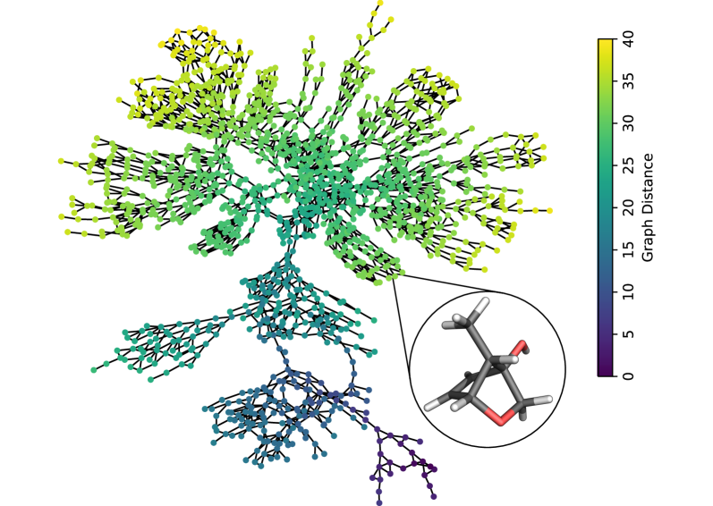
Figure 1: Reaction network considered in this study. Nodes represent three-dimensional molecular structures of constitutional isomers of the $\text{C}_{7}\text{H}_{10}\text{O}_{2}$ stoichiometry. Edges are drawn between two nodes if there is a transformation rule interconverting their molecular graphs. A node’s color represents its graph distance to a (randomly chosen) node in the network.

We calculate the SOAP kernel[96] $k(\mathbf{x},\mathbf{x}^{\prime})$ for every pair of structures in the data set. This measure of molecular similarity is suitable for a special class of molecular structures that we consider in this work: stable intermediates. In fact, many electronic structure methods ranging from Kohn–Sham DFT to single-reference coupled cluster models have been developed for this special type of stationary points on the Born–Oppenheimer potential energy hypersurface (PES). It is well-known that many of them will fail for dissociation processes (examples are wrong asymptotes of coupled cluster calculations and the Hartree–Fock dissociation error). Clearly, considering also structures away from stable intermediates would require an extension of the descriptor chosen for this work. However, such extensions are rather straightforward to define. Consider, for example, a multidimensional descriptor that also considers electronic structure information such as the gap between the highest occupied molecular orbital and the lowest unoccupied molecular orbital; see also the work of Kulik and co-workers.[99, 92, 100] Such an extension of the kernel would also improve its ability to capture long-range effects.

A special and important class of stationary points on the PES next to that of stable intermediates are transition-state structures, i.e., first-order saddle points on the PES. We would need to consider these structures in order to transgress the thermodynamic view of reaction networks and to approach kinetic modeling. Whereas this is beyond the scope of the present work, we note in passing that apart from the option to explicitly include information on the electronic structure of a given molecular structure (which would also allow one to consider different charge and spin states), we may treat transition-state structures as a new class of structures characterized by the fact that an electronically excited state is generally closer in energy than that is the case for stable intermediate. One may, therefore, keep intermediates and transition states (and species of different charge or spin multiplicity) in separate data sets in order to best account for these different types of electronic structures (e.g., closed-shell ground-state minima, ground-state bond-activated structures with a tendency for multiconfigurational nature, neutral vs. excess-charge species, and so forth).

If a set of intermediates on different PESs (but with the same charge and spin multiplicity) are encountered during the exploration, the smallest collection of atoms from which every molecule in the set can be constructed can be assembled. Then, upon comparison of two structures $x$ and $x^{\prime}$ from this set with the kernel $k(\mathbf{x},\mathbf{x}^{\prime})$, the atoms that are not needed to form either of the two would still be part of the comparison but in the form of idealized “isolated” species.[57] In this way, all comparisons between structures from this set are on equal footing.

3.2 Learning and Predictions

Calculating a thermodynamic property $P^{\text{ref}}(\mathbf{x})$ (e.g., the standard enthalpy of atomization) with accurate methods, such as G4MP2,[101] is computationally demanding. Statistical learning can be employed to improve a result of computationally (comparatively) inexpensive quantum chemical methods, $P^{\text{base}}(\mathbf{x})$, by predicting the error of a method with respect to some accurate reference result:

$$\Delta P^{\text{ref}}_{\text{base}}(\mathbf{x})=P^{\text{ref}}(\mathbf{x})-P^{\text{base}}(\mathbf{x}).$$ (18)

This strategy is often referred to as $\Delta$-machine learning.[102] It is based on the idea that inexpensive quantum chemical methods are able to describe a significant portion of the underlying physics (e.g., nuclear repulsion) but fail to capture more complex phenomena such as electron correlation. It is these effects that are then learned in a $\Delta$-machine learning approach. By design, $\Delta$-machine learning approaches require the evaluation of the inexpensive $P^{\text{base}}$ to arrive at the desired property.

In this work, we apply the $\Delta$-machine learning approach by learning the difference in the calculated standard enthalpy of atomization between G4MP2 and the density-functional approach with PBE[103] ($\Delta H^{\text{G4MP2}}_{\text{PBE}}$) as well as G4MP2 and the semiempirical model PM7[104] ($\Delta H^{\text{G4MP2}}_{\text{PM7}}$). We emphasize that the choice of inexpensive (here, PBE and PM7) and reference (here, G4MP2) method is to a certain degree arbitrary, and other choices work as well for our protocol (provided that the reference method has been demonstrated to be more accurate than the inexpensive models for the data set under consideration). The distributions of $\Delta H^{\text{G4MP2}}_{\text{PBE}}$ and $\Delta H^{\text{G4MP2}}_{\text{PM7}}$ in the data set are shown in Fig. 2 (see the Computational Methodology for details). Due to the more approximate nature of the semiempirical PM7 method compared to the PBE density functional, the distribution of $\Delta H^{\text{G4MP2}}_{\text{PM7}}$ is much wider than that of $\Delta H^{\text{G4MP2}}_{\text{PBE}}$.

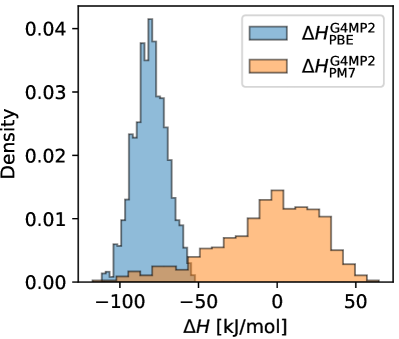
Figure 2: Distributions of $\Delta H^{\text{G4MP2}}_{\text{PBE}}$ and $\Delta H^{\text{G4MP2}}_{\text{PM7}}$ for the data set.

We calculate the SOAP kernel[96] $k(\mathbf{x},\mathbf{x}^{\prime})$ for every pair of structures in the data set. This kernel also provides a definition of the distance between two structures[57]

$$d(\mathbf{x},\mathbf{x}^{\prime})=\sqrt{2-2k(\mathbf{x},\mathbf{x}^{\prime})}.$$ (19)

To illustrate the notion of distance in a reaction network, a subnetwork of the whole reaction network is arranged according to $d(\mathbf{x},\mathbf{x}^{\prime})$ in Fig. 3, where $\mathbf{x}$ is some reactant and $\mathbf{x}^{\prime}$ a possible product.

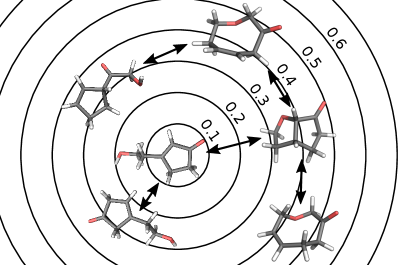
Figure 3: Illustration of the distance metric in eq. (19) introduced by the kernel at the example of a reaction subnetwork. The contour lines represent the distance $d(\mathbf{x},\mathbf{x}^{\prime})$ between the reactant in the center ($\mathbf{x}$) and possible reaction products present in the data set ($\mathbf{x}^{\prime}$). Double arrows are drawn between structures if there is a transformation rule interconverting their molecular graphs.

For both targets separately, we trained a GP on randomly selected subsets of different size and employed the remaining structures as an out-of-sample validation set. The GP’s hyperparameters are optimized by maximizing the marginal likelihood. For predictions on the validation set, we calculated the mean absolute error (MAE),

$$\text{MAE}=\frac{1}{N}\sum_{i=1}^{N}|\bar{\mathcal{T}}(\mathbf{x}_{i})-\mathcal{T}(\mathbf{x}_{i})|,$$ (20)

and root-mean-square error (RMSE),

$$\text{RMSE}=\sqrt{\frac{1}{N}\sum_{i=1}^{N}\left(\bar{\mathcal{T}}(\mathbf{x}_{i})-\mathcal{T}(\mathbf{x}_{i})\right)^{2}},$$ (21)

where $N$ is the size of the out-of-sample validation set, $\bar{\mathcal{T}}(\mathbf{x}_{i})$ the prediction mean, and $\mathcal{T}(\mathbf{x}_{i})$ the target value. To better assess the behavior of the GP, we also calculated the MAE (MAE${}_{\text{ref}}$) and the RMSE (RMSE${}_{\text{ref}}$) of a trivial statistical model that simply predicts the mean of the training data set for every test input. In addition, to guarantee the accuracy of the error estimates, we calculated the percentage of predictions $r_{\text{cb}}$ for which the target lies outside of the 95% confidence band given by $\bar{\mathcal{T}}(\mathbf{x}_{i})\pm 2\sigma(\mathbf{x}_{i})$. We repeated this process 25 times to ensure that the average of the above metrics converged. The average properties are summarized in Table 1. It can be seen that the prediction accuracy improves significantly with the size of the training data set. When comparing the MAE and the RMSE to the MAE${}_{\text{ref}}$ and the RMSE${}_{\text{ref}}$, respectively, it becomes evident that the use of a GP can be justified only for training data set sizes of 200 and larger. It can also be seen that the prediction error of $\Delta H^{\text{G4MP2}}_{\text{PM7}}$ is larger than that of $\Delta H^{\text{G4MP2}}_{\text{PBE}}$. This can be explained by the approximate nature of the semiempirical PM7 method (see Fig. 2). Nonetheless, the results suggest that the prediction error estimates are reliable as $r_{\text{cb}}$ is close to 5% for all data set sizes and targets.

Table 1: Mean absolute error (MAE), reference MAE (MAE${}_{\text{ref}}$), root-mean-square error (RMSE), reference RMSE (RMSE${}_{\text{ref}}$) (in kJ/mol), and $r_{\text{cb}}$ of GP predictions on $\Delta H^{\text{G4MP2}}_{\text{PBE}}$ and $\Delta H^{\text{G4MP2}}_{\text{PM7}}$ for different training data set sizes.

Size	Target	MAE	MAE${}_{\text{ref}}$	RMSE	RMSE${}_{\text{ref}}$	$r_{\text{cb}}$
50	$\Delta H^{\text{G4MP2}}_{\text{PBE}}$	7.82	8.42	9.71	10.53	5.24
	$\Delta H^{\text{G4MP2}}_{\text{PM7}}$	21.61	26.24	27.86	33.13	6.40
100	$\Delta H^{\text{G4MP2}}_{\text{PBE}}$	7.30	8.42	9.03	10.53	4.53
	$\Delta H^{\text{G4MP2}}_{\text{PM7}}$	19.15	26.16	25.01	32.99	6.03
200	$\Delta H^{\text{G4MP2}}_{\text{PBE}}$	6.37	8.40	7.84	10.50	3.52
	$\Delta H^{\text{G4MP2}}_{\text{PM7}}$	15.71	26.12	21.06	32.97	6.48
500	$\Delta H^{\text{G4MP2}}_{\text{PBE}}$	4.42	8.39	5.45	10.48	3.83
	$\Delta H^{\text{G4MP2}}_{\text{PM7}}$	8.31	26.16	11.25	32.99	6.21
1000	$\Delta H^{\text{G4MP2}}_{\text{PBE}}$	2.90	8.37	3.64	10.45	4.26
	$\Delta H^{\text{G4MP2}}_{\text{PM7}}$	4.64	26.15	6.21	32.91	4.74

For the study of chemical reactivity, not enthalpies of formation but (free) enthalpy differences between intermediates are usually of interest. From a GP trained on a molecular target, predictions on differences with respect to that target between molecular structures are readily available through eqs. (12) and (13). For both targets separately, we trained a GP on randomly selected subsets of different size and then predicted relative energies between the remaining structures. This process was repeated 25 times to obtain converged means of the MAE, RMSE, and $r_{\text{cb}}$. From the results shown in Table 2, it can be seen that the MAE and the RMSE decrease rapidly with data set size; however, the accuracy is lower than that of predictions on the standard enthalpy of atomization. Nonetheless, $r_{\text{cb}}$ indicates that the error estimates remain reliable.

Table 2: Mean absolute error (MAE), root-mean-square error (RMSE) (in kJ/mol), and $r_{\text{cb}}$ of predictions on differences in the standard enthalpy between molecular structures from GPs trained on targets $\Delta H^{\text{G4MP2}}_{\text{PBE}}$ and $\Delta H^{\text{G4MP2}}_{\text{PM7}}$.

Size	Target	MAE	RMSE	$r_{\text{cb}}$
50	$\Delta H^{\text{G4MP2}}_{\text{PBE}}$	10.96	13.67	5.35
	$\Delta H^{\text{G4MP2}}_{\text{PM7}}$	30.69	39.11	6.34
100	$\Delta H^{\text{G4MP2}}_{\text{PBE}}$	10.22	12.74	4.91
	$\Delta H^{\text{G4MP2}}_{\text{PM7}}$	27.54	35.26	5.56
200	$\Delta H^{\text{G4MP2}}_{\text{PBE}}$	8.88	11.07	4.22
	$\Delta H^{\text{G4MP2}}_{\text{PM7}}$	22.95	29.75	5.81
500	$\Delta H^{\text{G4MP2}}_{\text{PBE}}$	6.17	7.70	4.37
	$\Delta H^{\text{G4MP2}}_{\text{PM7}}$	12.13	15.88	5.96
1000	$\Delta H^{\text{G4MP2}}_{\text{PBE}}$	4.09	5.15	4.53
	$\Delta H^{\text{G4MP2}}_{\text{PM7}}$	6.72	8.78	5.36

Hence, we demonstrated that GPs are capable of learning molecular properties of molecular structures with reliable error estimates. Furthermore, relative molecular properties can be predicted with sufficient accuracy employing a statistical model trained on individual molecular properties.

3.3 Error-Controlled Exploration

For the consecutive discovery of intermediates in the exploration of a chemical system, we generated sequences of nodes from our reaction network. Whereas all nodes are already known in our example network, an actual exploration procedure would expand the network in a continuous fashion (see refs.  105 and 106). Starting from a random initial node in the reaction network, the remaining nodes were visited in the order of their graph distance to the initial node (see Fig. 1). Nodes with the same graph distance were discovered in a random order. Next, the error-controlled exploration strategy outlined in section 2.4 was applied. Here, the initial data set consisted of the first $m=75$ explored nodes. The explorations were separately performed for the targets $\Delta H^{\text{G4MP2}}_{\text{PBE}}$ and $\Delta H^{\text{G4MP2}}_{\text{PM7}}$. For each target, three different runs with different variance thresholds were carried out. Results for the exploration with targets $\Delta H^{\text{G4MP2}}_{\text{PBE}}$ and $\Delta H^{\text{G4MP2}}_{\text{PM7}}$ (on the same sequence) are shown in Figs. 4 and 5, respectively.

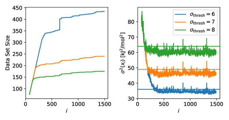
Figure 4: Size of the training data set (left) and prediction variance on the enthalpy of atomization (right) for the $i$th structure in an exploration employing the PBE functional and G4MP2 as the reference.

From Fig. 4 it can be seen that the size of the training data set initially increases. This is due to the low prediction confidence at the beginning of the exploration. The data set increases until the prediction uncertainty is below $\sigma_{\text{thresh}}^{2}$ (shown as a horizontal line in Fig. 4, right). This is the point at which the predictions made by the GP are trusted for the first time. If, however, the exploration reaches regions of chemical space that are distant to the previously explored ones, the confidence will drop and new reference calculations will be required. This can be observed in Fig. 4, right, where the variance exceeds $\sigma_{\text{thresh}}^{2}$. Naturally, the total number of reference calculations for the entire exploration depends on the target and $\sigma_{\text{thresh}}^{2}$. Finally, it can be seen that the backtracking mechanism described in Section 2.4 is indeed necessary. In Fig. 4, for $\sigma_{\text{thresh}}=6$ kJ/mol at $i=651$, the GP is updated and some predictions which previously were inside the confidence bound now lie outside of it. Consequently, data points are added to the data set followed by an update of the GP until all predictions are within the confidence bound.

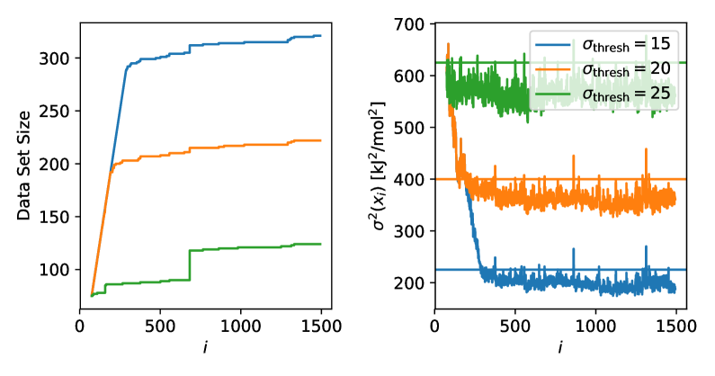
Figure 5: Size of the training data set (left) and prediction variance on the enthalpy of atomization (right) for the $i$th structure in an exploration employing PM7 and G4MP2 as the reference.

Fig. 5 shows that a larger data set is required for the target $\Delta H^{\text{G4MP2}}_{\text{PM7}}$ to reach a standard deviation of 15 kJ/mol than that for the target $\Delta H^{\text{G4MP2}}_{\text{PBE}}$ to reach a standard deviation of 8 kJ/mol. This finding is in accordance with the results presented in Table 1. Calculation of the enthalpy of atomization is faster with PM7 than that with PBE by about an order of magnitude (for the systems studied in this work). However, because the exploration with PM7 as the base method requires far more computationally expensive G4MP2 reference calculations (which take more than three orders of magnitude longer than PBE calculations for the systems studied in this work), the overall exploration takes longer with PM7 than that with PBE as the base method. We note that the time required for the evaluation of the kernel and GP predictions is negligible for data sets of this size. This illustrates the philosophy of the $\Delta$-machine learning approach that should work more efficiently for the physically more reliable model (in our case, this is PBE). As a result, given a required confidence level, a trade-off needs to be found between the required number of reference calculations and the computational effort of the base method. Results of an exploration starting from a different node are provided in the Supporting Information.

4 Conclusions

In this work, a novel approach for the rolling improvement of quantum chemical results through the application of GPs is presented. By learning the error of an efficient quantum chemical method with respect to some reference method of higher accuracy, we obtained accurate standard enthalpies of formation for configurational isomers of $\text{C}_{7}\text{H}_{10}\text{O}_{2}$ stoichiometry. Accurate differences in standard enthalpy between isomers are accessible as well. Furthermore, we showed that the uncertainty estimates provided by our predictive model for both the standard enthalpy of formation of molecules and the difference in the standard enthalpy between molecules are reliable. If the uncertainty associated with a particular calculation is above a given threshold, then the chosen reference method will be employed to produce additional reference data. In this way, reference calculations are performed only if truly necessary, i.e., if regions of chemical space unknown to our model are approached and explored. The approach presented in this work is independent of the chosen molecular descriptor and can also be carried out with more involved machine learning methods that provide error estimates. In addition, we emphasize that our approach is independent of the chosen electronic structure methods, ranging from semiempirical and tight-binding models to multiconfigurational approaches with multireference perturbation theory. Through backtracking, previous predictions are validated by the updated model to ensure that uncertainties remain within the given confidence bound.

Our approach will be beneficial for mechanism-exploration algorithms,[107, 108, 109, 106, 110, 111, 112] of which our Chemoton[105] algorithm is one example designed to be applicable to molecules from the whole periodic table of elements. The combination with our KiNetX[113] algorithm for kinetic modeling under uncertainty propagation is currently being investigated in our laboratory. In this way, reliable first-principles explorations of those portions of chemical reaction space that are relevant for a specific chemical problem will become accessible. Obviously, this will require the accessibility of accurate reference calculations on demand. For instance, our multiconfigurational diagnostic[114] will allow one to decide on the singlereference vs. multireference nature of the molecular structure subjected to a reference calculation. For single-reference cases, explicitly correlated, local coupled cluster calculations[15] are the method of choice as they can be easily launched in an automated manner and are known to be highly accurate. For multiconfigurational cases, automated complete active space-type calculations can be launched with our fully automated procedure[115] for the selection of active orbital spaces[116, 117, 118].

Computational Methodology

The data set employed in this study is a subset of the GDB-17 data set.[119] All G4 geometries were taken from ref.  98. The list of unique identifiers of the structures contained in this data set can be found in the Supporting Information. G4MP2 enthalpies of atomization were also taken from ref.  98. DFT enthalpies of atomization were based on electronic energies obtained with the PBE exchange-correlation functional[103] and a double-$\zeta$ basis.[120] DFT calculations were performed with the program packages Q-Chem (version 4.3).[121] Vibrational frequencies and rotational constants were taken from ref.  98. Accordingly, $\Delta H^{\text{G4MP2}}_{\text{PBE}}$ is given by the difference in G4MP2 and PBE electronic energies of atomization as the nuclear contributions cancel in this setup. By contrast, PM7 enthalpies of atomization were calculated from enthalpies of formation obtained with the MOPAC program (version 2016).[122]

The SOAP average kernel was evaluated with the glosim package.[57] Following previous work,[96, 97] we chose an exponent of $\zeta=4.0$. In addition, we set the Gaussian width parameter to be $\sigma=0.3\,\textup{\AA}$ and the cutoff radius to be $R_{\text{cut}}=4.0\,\textup{\AA}$. Furthermore, we chose the number of radial and angular functions to be 12 and 10, respectively. Our model would likely benefit from an exhaustive search over hyperparameters; however, consistent with previous findings,[57] the performance of the kernel is not highly sensitive to the chosen set of parameters.

GP predictions were carried out with the library GPy.[123] Data analysis and visualization were performed with the Python libraries pandas[124] and matplotlib[125], respectively. The graphical representation of the reaction network was created by the Graphviz program.[126]

Supporting Information

In the supporting information of the published article, the data set and the reaction network employed in this work can be found. In addition, it contains a figure on the GPs’ prediction accuracy. Finally, the results of an additional exploration are provided. This exploration differs in the initial node (i.e., the starting point of the exploration) from the one discussed in the main text.

References

- [1] Claeyssens, F.; Harvey, J. N.; Manby, F. R.; Mata, R. A.; Mulholland, A. J.; Ranaghan, K. E.; Schütz, M.; Thiel, S.; Thiel, W.; Werner, H.-J. High-Accuracy Computation of Reaction Barriers in Enzymes, Angew. Chem. Int. Ed. 2006, 45, 6856-6859.
- [2] Hohenberg, P.; Kohn, W. Inhomogeneous Electron Gas, Phys. Rev. 1964, 136, B864-B871.
- [3] Lieb, E. H. Density Functionals for Coulomb Systems, Int. J. Quantum Chem. 1983, 24, 243-277.
- [4] Mardirossian, N.; Head-Gordon, M. Thirty Years of Density Functional Theory in Computational Chemistry: An Overview and Extensive Assessment of 200 Density Functionals, Mol. Phys. 2017, 115, 2315-2372.
- [5] Perdew, J. P.; Schmidt, K.; Van Doren, V.; Van Alsenoy, C.; Geerlings, P. Jacob’s Ladder of Density Functional Approximations for the Exchange-Correlation Energy, AIP Conf. Proc. 2001, 577, 1-20.
- [6] Niu, S.; Hall, M. B. Theoretical Studies on Reactions of Transition-Metal Complexes, Chem. Rev. 2000, 100, 353-406.
- [7] Schultz, N. E.; Zhao, Y.; Truhlar, D. G. Density Functionals for Inorganometallic and Organometallic Chemistry, J. Phys. Chem. A 2005, 109, 11127-11143.
- [8] Furche, F.; Perdew, J. P. The Performance of Semilocal and Hybrid Density Functionals in 3d Transition-Metal Chemistry, J. Chem. Phys. 2006, 124, 044103.
- [9] Riley, K. E.; Merz, K. M. Assessment of Density Functional Theory Methods for the Computation of Heats of Formation and Ionization Potentials of Systems Containing Third Row Transition Metals, J. Phys. Chem. A 2007, 111, 6044-6053.
- [10] Jiang, W.; DeYonker, N. J.; Determan, J. J.; Wilson, A. K. Toward Accurate Theoretical Thermochemistry of First Row Transition Metal Complexes, J. Phys. Chem. A 2012, 116, 870-885.
- [11] Weymuth, T.; Couzijn, E. P. A.; Chen, P.; Reiher, M. New Benchmark Set of Transition-Metal Coordination Reactions for the Assessment of Density Functionals, J. Chem. Theory Comput. 2014, 10, 3092-3103.
- [12] Weymuth, T.; Reiher, M. Systematic Dependence of Transition-Metal Coordination Energies on Density-Functional Parametrizations, Int. J. Quantum Chem. 2015, 115, 90-98.
- [13] Liu, C.; Liu, T.; Hall, M. B. Influence of the Density Functional and Basis Set on the Relative Stabilities of Oxygenated Isomers of Diiron Models for the Active Site of [FeFe]-Hydrogenase, J. Chem. Theory Comput. 2015, 11, 205-214.
- [14] Husch, T.; Freitag, L.; Reiher, M. Calculation of Ligand Dissociation Energies in Large Transition-Metal Complexes, J. Chem. Theory Comput. 2018, 14, 2456-2468.
- [15] Ma, Q.; Werner, H.-J. Explicitly Correlated Local Coupled-Cluster Methods Using Pair Natural Orbitals, WIREs Comput. Mol. Sci. 2018, e1371.
- [16] Pople, J. A.; Head-Gordon, M.; Fox, D. J.; Raghavachari, K.; Curtiss, L. A. Gaussian-1 Theory: A General Procedure for Prediction of Molecular Energies, J. Chem. Phys. 1989, 90, 5622-5629.
- [17] Curtiss, L. A.; Raghavachari, K.; Trucks, G. W.; Pople, J. A. Gaussian-2 Theory for Molecular Energies of First- and Second-row Compounds, J. Chem. Phys. 1991, 94, 7221-7230.
- [18] Curtiss, L. A.; Raghavachari, K.; Redfern, P. C.; Pople, J. A. Assessment of Gaussian-2 and Density Functional Theories for the Computation of Enthalpies of Formation, J. Chem. Phys. 1997, 106, 1063-1079.
- [19] Curtiss, L. A.; Raghavachari, K.; Redfern, P. C.; Pople, J. A. Assessment of Gaussian-3 and Density Functional Theories for a Larger Experimental Test Set, J. Chem. Phys. 2000, 112, 7374-7383.
- [20] Lynch, B. J.; Truhlar, D. G. Robust and Affordable Multicoefficient Methods for Thermochemistry and Thermochemical Kinetics: The MCCM/3 Suite and SAC/3, J. Phys. Chem. A 2003, 107, 3898-3906.
- [21] Lynch, B. J.; Truhlar, D. G. Small Representative Benchmarks for Thermochemical Calculations, J. Phys. Chem. A 2003, 107, 8996-8999.
- [22] Lynch, B. J.; Zhao, Y.; Truhlar, D. G. Effectiveness of Diffuse Basis Functions for Calculating Relative Energies by Density Functional Theory, J. Phys. Chem. A 2003, 107, 1384-1388.
- [23] Zhao, Y.; Lynch, B. J.; Truhlar, D. G. Development and Assessment of a New Hybrid Density Functional Model for Thermochemical Kinetics, J. Phys. Chem. A 2004, 108, 2715-2719.
- [24] Schultz, N. E.; Zhao, Y.; Truhlar, D. G. Databases for Transition Element Bonding: Metal-Metal Bond Energies and Bond Lengths and Their Use To Test Hybrid, Hybrid Meta, and Meta Density Functionals and Generalized Gradient Approximations, J. Phys. Chem. A 2005, 109, 4388-4403.
- [25] Zhao, Y.; González-García, N.; Truhlar, D. G. Benchmark Database of Barrier Heights for Heavy Atom Transfer, Nucleophilic Substitution, Association, and Unimolecular Reactions and Its Use to Test Theoretical Methods, J. Phys. Chem. A 2005, 109, 2012-2018.
- [26] Zhao, Y.; Truhlar, D. G. Benchmark Databases for Nonbonded Interactions and Their Use To Test Density Functional Theory, J. Chem. Theory Comput. 2005, 1, 415-432.
- [27] Zhao, Y.; Truhlar, D. G. Benchmark Data for Interactions in Zeolite Model Complexes and Their Use for Assessment and Validation of Electronic Structure Methods, J. Phys. Chem. C 2008, 112, 6860-6868.
- [28] Zhao, Y.; Truhlar, D. G. Benchmark Energetic Data in a Model System for Grubbs II Metathesis Catalysis and Their Use for the Development, Assessment, and Validation of Electronic Structure Methods, J. Chem. Theory Comput. 2009, 5, 324-333.
- [29] Korth, M.; Grimme, S. “Mindless” DFT Benchmarking, J. Chem. Theory Comput. 2009, 5, 993-1003.
- [30] Goerigk, L.; Grimme, S. A General Database for Main Group Thermochemistry, Kinetics, and Noncovalent Interactions - Assessment of Common and Reparameterized (Meta-)GGA Density Functionals, J. Chem. Theory Comput. 2010, 6, 107-126.
- [31] Goerigk, L.; Grimme, S. Efficient and Accurate Double-Hybrid-Meta-GGA Density Functionals—Evaluation with the Extended GMTKN30 Database for General Main Group Thermochemistry, Kinetics, and Noncovalent Interactions, J. Chem. Theory Comput. 2011, 7, 291-309.
- [32] Salomon, O.; Reiher, M.; Hess, B. A. Assertion and Validation of the Performance of the B3LYP⋆ Functional for the First Transition Metal Row and the G2 Test Set, J. Chem. Phys. 2002, 117, 4729-4737.
- [33] Curtiss, L. A.; Redfern, P. C.; Raghavachari, K. Assessment of Gaussian-3 and Density-Functional Theories on the G3/05 Test Set of Experimental Energies, J. Chem. Phys. 2005, 123, 124107.
- [34] Cohen, A. J.; Mori-Sánchez, P.; Yang, W. Insights into Current Limitations of Density Functional Theory, Science 2008, 321, 792-794.
- [35] Pernot, P.; Civalleri, B.; Presti, D.; Savin, A. Prediction Uncertainty of Density Functional Approximations for Properties of Crystals with Cubic Symmetry, J. Phys. Chem. A 2015, 119, 5288-5304.
- [36] Simm, G. N.; Reiher, M. Systematic Error Estimation for Chemical Reaction Energies, J. Chem. Theory Comput. 2016, 12, 2762-2773.
- [37] Simm, G. N.; Proppe, J.; Reiher, M. Error Assessment of Computational Models in Chemistry, Chimia 2017, 71, 202-208.
- [38] Mortensen, J. J.; Kaasbjerg, K.; Frederiksen, S. L.; Nørskov, J. K.; Sethna, J. P.; Jacobsen, K. W. Bayesian Error Estimation in Density-Functional Theory, Phys. Rev. Lett. 2005, 95, 216401.
- [39] Brown, K. S.; Sethna, J. P. Statistical Mechanical Approaches to Models with Many Poorly Known Parameters, Phys. Rev. E 2003, 68, 021904.
- [40] Frederiksen, S. L.; Jacobsen, K. W.; Brown, K. S.; Sethna, J. P. Bayesian Ensemble Approach to Error Estimation of Interatomic Potentials, Phys. Rev. Lett. 2004, 93, 165501.
- [41] Petzold, V.; Bligaard, T.; Jacobsen, K. W. Construction of New Electronic Density Functionals with Error Estimation Through Fitting, Top. Catal. 2012, 55, 402-417.
- [42] Wellendorff, J.; Lundgaard, K. T.; Møgelhøj, A.; Petzold, V.; Landis, D. D.; Nørskov, J. K.; Bligaard, T.; Jacobsen, K. W. Density Functionals for Surface Science: Exchange-Correlation Model Development with Bayesian Error Estimation, Phys. Rev. B 2012, 85, 235149.
- [43] Wellendorff, J.; Lundgaard, K. T.; Jacobsen, K. W.; Bligaard, T. mBEEF: An Accurate Semi-Local Bayesian Error Estimation Density Functional, J. Chem. Phys. 2014, 140, 144107.
- [44] Pandey, M.; Jacobsen, K. W. Heats of Formation of Solids with Error Estimation: The mBEEF Functional with and without Fitted Reference Energies, Phys. Rev. B 2015, 91, 235201.
- [45] Pernot, P. The Parameter Uncertainty Inflation Fallacy, J. Chem. Phys. 2017, 147, 104102.
- [46] Aldegunde, M.; Kermode, J. R.; Zabaras, N. Development of an Exchange–correlation Functional with Uncertainty Quantification Capabilities for Density Functional Theory, J. Comput. Phys. 2016, 311, 173-195.
- [47] Sutton, J. E.; Vlachos, D. G. Effect of Errors in Linear Scaling Relations and Brønsted–Evans–Polanyi Relations on Activity and Selectivity Maps, J. Catal. 2016, 338, 273-283.
- [48] Behler, J.; Parrinello, M. Generalized Neural-Network Representation of High-Dimensional Potential-Energy Surfaces, Phys. Rev. Lett. 2007, 98, 146401.
- [49] Balabin, R. M.; Lomakina, E. I. Neural Network Approach to Quantum-Chemistry Data: Accurate Prediction of Density Functional Theory Energies, J. Chem. Phys. 2009, 131, 074104.
- [50] Bartók, A. P.; Payne, M. C.; Kondor, R.; Csányi, G. Gaussian Approximation Potentials: The Accuracy of Quantum Mechanics, without the Electrons, Phys. Rev. Lett. 2010, 104, 136403.
- [51] Rupp, M.; Tkatchenko, A.; Müller, K.-R.; von Lilienfeld, O. A. Fast and Accurate Modeling of Molecular Atomization Energies with Machine Learning, Phys. Rev. Lett. 2012, 108, 058301.
- [52] Montavon, G.; Rupp, M.; Gobre, V.; Vazquez-Mayagoitia, A.; Hansen, K.; Tkatchenko, A.; Müller, K.-R.; von Lilienfeld, O. A. Machine Learning of Molecular Electronic Properties in Chemical Compound Space, New J. Phys. 2013, 15, 095003.
- [53] Bartók, A. P.; Gillan, M. J.; Manby, F. R.; Csányi, G. Machine-Learning Approach for One- and Two-Body Corrections to Density Functional Theory: Applications to Molecular and Condensed Water, Phys. Rev. B 2013, 88, 054104.
- [54] Hansen, K.; Montavon, G.; Biegler, F.; Fazli, S.; Rupp, M.; Scheffler, M.; von Lilienfeld, O. A.; Tkatchenko, A.; Müller, K.-R. Assessment and Validation of Machine Learning Methods for Predicting Molecular Atomization Energies, J. Chem. Theory Comput. 2013, 9, 3404-3419.
- [55] Schütt, K. T.; Glawe, H.; Brockherde, F.; Sanna, A.; Müller, K. R.; Gross, E. K. U. How to Represent Crystal Structures for Machine Learning: Towards Fast Prediction of Electronic Properties, Phys. Rev. B 2014, 89, 205118.
- [56] Dral, P. O.; von Lilienfeld, O. A.; Thiel, W. Machine Learning of Parameters for Accurate Semiempirical Quantum Chemical Calculations, J. Chem. Theory Comput. 2015, 11, 2120-2125.
- [57] De, S.; Bartók, A. P.; Csányi, G.; Ceriotti, M. Comparing Molecules and Solids across Structural and Alchemical Space, Phys. Chem. Chem. Phys. 2016, 18, 13754-13769.
- [58] Faber, F. A.; Hutchison, L.; Huang, B.; Gilmer, J.; Schoenholz, S. S.; Dahl, G. E.; Vinyals, O.; Kearnes, S.; Riley, P. F.; von Lilienfeld, O. A. Prediction Errors of Molecular Machine Learning Models Lower than Hybrid DFT Error, J. Chem. Theory Comput. 2017, 13, 5255-5264.
- [59] Chmiela, S.; Tkatchenko, A.; Sauceda, H. E.; Poltavsky, I.; Schütt, K. T.; Müller, K.-R. Machine Learning of Accurate Energy-Conserving Molecular Force Fields, Sci. Adv. 2017, 3, e1603015.
- [60] Schütt, K. T.; Arbabzadah, F.; Chmiela, S.; Müller, K. R.; Tkatchenko, A. Quantum-Chemical Insights from Deep Tensor Neural Networks, Nat. Commun. 2017, 8, 13890.
- [61] Bartók, A. P.; De, S.; Poelking, C.; Bernstein, N.; Kermode, J. R.; Csányi, G.; Ceriotti, M. Machine Learning Unifies the Modeling of Materials and Molecules, Sci. Adv. 2017, 3, e1701816.
- [62] Behler, J.; Martoňák, R.; Donadio, D.; Parrinello, M. Metadynamics Simulations of the High-Pressure Phases of Silicon Employing a High-Dimensional Neural Network Potential, Phys. Rev. Lett. 2008, 100, 185501.
- [63] Handley, C. M.; Popelier, P. L. A. Potential Energy Surfaces Fitted by Artificial Neural Networks, J. Phys. Chem. A 2010, 114, 3371-3383.
- [64] Botu, V.; Ramprasad, R. Adaptive Machine Learning Framework to Accelerate Ab Initio Molecular Dynamics, Int. J. Quantum Chem. 2015, 115, 1074-1083.
- [65] Hansen, K.; Biegler, F.; Ramakrishnan, R.; Pronobis, W.; von Lilienfeld, O. A.; Müller, K.-R.; Tkatchenko, A. Machine Learning Predictions of Molecular Properties: Accurate Many-Body Potentials and Nonlocality in Chemical Space, J. Phys. Chem. Lett. 2015, 6, 2326-2331.
- [66] Shen, L.; Wu, J.; Yang, W. Multiscale Quantum Mechanics/Molecular Mechanics Simulations with Neural Networks, J. Chem. Theory Comput. 2016, 12, 4934-4946.
- [67] Li, Y.; Li, H.; Pickard, F. C.; Narayanan, B.; Sen, F. G.; Chan, M. K. Y.; Sankaranarayanan, S. K. R. S.; Brooks, B. R.; Roux, B. Machine Learning Force Field Parameters from Ab Initio Data, J. Chem. Theory Comput. 2017, 13, 4492-4503.
- [68] Bleiziffer, P.; Schaller, K.; Riniker, S. Machine Learning of Partial Charges Derived from High-Quality Quantum-Mechanical Calculations, J. Chem. Inf. Model. 2018, 58, 579-590.
- [69] Chmiela, S.; Sauceda, H. E.; Müller, K.-R.; Tkatchenko, A. Towards Exact Molecular Dynamics Simulations with Machine-Learned Force Fields, 2018, arXiv:1802.09238.
- [70] Gómez-Bombarelli, R.; Wei, J. N.; Duvenaud, D.; Hernández-Lobato, J. M.; Sánchez-Lengeling, B.; Sheberla, D.; Aguilera-Iparraguirre, J.; Hirzel, T. D.; Adams, R. P.; Aspuru-Guzik, A. Automatic Chemical Design Using a Data-Driven Continuous Representation of Molecules, ACS Cent. Sci. 2018, 4, 268-276.
- [71] Zhou, Z.; Li, X.; Zare, R. N. Optimizing Chemical Reactions with Deep Reinforcement Learning, ACS Cent. Sci. 2017, 3, 1337-1344.
- [72] Altae-Tran, H.; Ramsundar, B.; Pappu, A. S.; Pande, V. Low Data Drug Discovery with One-Shot Learning, ACS Cent. Sci. 2017, 3, 283-293.
- [73] Liu, B.; Ramsundar, B.; Kawthekar, P.; Shi, J.; Gomes, J.; Luu Nguyen, Q.; Ho, S.; Sloane, J.; Wender, P.; Pande, V. Retrosynthetic Reaction Prediction Using Neural Sequence-to-Sequence Models, ACS Cent. Sci. 2017, 3, 1103-1113.
- [74] Segler, M. H. S.; Kogej, T.; Tyrchan, C.; Waller, M. P. Generating Focused Molecule Libraries for Drug Discovery with Recurrent Neural Networks, ACS Cent. Sci. 2018, 4, 120-131.
- [75] Kayala, M. A.; Azencott, C.-A.; Chen, J. H.; Baldi, P. Learning to Predict Chemical Reactions, J. Chem. Inf. Model. 2011, 51, 2209-2222.
- [76] Sadowski, P.; Fooshee, D.; Subrahmanya, N.; Baldi, P. Synergies Between Quantum Mechanics and Machine Learning in Reaction Prediction, J. Chem. Inf. Model. 2016, 56, 2125-2128.
- [77] Wei, J. N.; Duvenaud, D.; Aspuru-Guzik, A. Neural Networks for the Prediction of Organic Chemistry Reactions, ACS Cent. Sci. 2016, 2, 725-732.
- [78] Raccuglia, P.; Elbert, K. C.; Adler, P. D. F.; Falk, C.; Wenny, M. B.; Mollo, A.; Zeller, M.; Friedler, S. A.; Schrier, J.; Norquist, A. J. Machine-Learning-Assisted Materials Discovery Using Failed Experiments, Nature 2016, 533, 73-76.
- [79] Segler, M. H. S.; Waller, M. P. Neural-Symbolic Machine Learning for Retrosynthesis and Reaction Prediction, Chem. Eur. J. 2017, 23, 5966-5971.
- [80] Jin, W.; Coley, C.; Barzilay, R.; Jaakkola, T. Predicting Organic Reaction Outcomes with Weisfeiler-Lehman Network. In Advances in Neural Information Processing Systems 30; Guyon, I.; Luxburg, U. V.; Bengio, S.; Wallach, H.; Fergus, R.; Vishwanathan, S.; Garnett, R., Eds.; Curran Associates, Inc.: 2017.
- [81] Fooshee, D.; Mood, A.; Gutman, E.; Tavakoli, M.; Urban, G.; Liu, F.; Huynh, N.; Van Vranken, D.; Baldi, P. Deep Learning for Chemical Reaction Prediction, Mol. Syst. Des. Eng. 2018, 3, 442-452.
- [82] Bradshaw, J.; Kusner, M. J.; Paige, B.; Segler, M. H. S.; Hernández-Lobato, J. M. Predicting Electron Paths, 2018, arXiv:1805.10970.
- [83] Ahneman, D. T.; Estrada, J. G.; Lin, S.; Dreher, S. D.; Doyle, A. G. Predicting Reaction Performance in C–N Cross-Coupling Using Machine Learning, Science 2018, eaar5169.
- [84] Rupp, M. Machine Learning for Quantum Mechanics in a Nutshell, Int. J. Quantum Chem. 2015, 115, 1058-1073.
- [85] Ramakrishnan, R.; Lilienfeld, O. A. Machine Learning, Quantum Chemistry, and Chemical Space. In Reviews in Computational Chemistry; Wiley-Blackwell: 2017, Vol. 30.
- [86] Csányi, G.; Albaret, T.; Payne, M. C.; De Vita, A. “Learn on the Fly”: A Hybrid Classical and Quantum-Mechanical Molecular Dynamics Simulation, Phys. Rev. Lett. 2004, 93, 175503.
- [87] Li, Z.; Kermode, J. R.; De Vita, A. Molecular Dynamics with On-the-Fly Machine Learning of Quantum-Mechanical Forces, Phys. Rev. Lett. 2015, 114, 096405.
- [88] Glielmo, A.; Sollich, P.; De Vita, A. Accurate Interatomic Force Fields via Machine Learning with Covariant Kernels, Phys. Rev. B 2017, 95, 214302.
- [89] Glielmo, A.; Zeni, C.; De Vita, A. Efficient Non-Parametric n-Body Force Fields from Machine Learning, 2018, arXiv:1801.04823.
- [90] Ulissi, Z. W.; Medford, A. J.; Bligaard, T.; Nørskov, J. K. To Address Surface Reaction Network Complexity Using Scaling Relations Machine Learning and DFT Calculations, Nat. Commun. 2017, 8, 14621.
- [91] Peterson, A. A.; Christensen, R.; Khorshidi, A. Addressing Uncertainty in Atomistic Machine Learning, Phys. Chem. Chem. Phys. 2017, 19, 10978-10985.
- [92] Janet, J. P.; Kulik, H. J. Resolving Transition Metal Chemical Space: Feature Selection for Machine Learning and Structure–Property Relationships, J. Phys. Chem. A 2017, 121, 8939-8954.
- [93] Rasmussen, C. E.; Williams, C. K. I. Gaussian Processes for Machine Learning; MIT Press: Cambridge, MA, 2006.
- [94] Mercer, J. XVI. Functions of Positive and Negative Type, and Their Connection the Theory of Integral Equations, Phil. Trans. R. Soc. Lond. A 1909, 209, 415-446.
- [95] Ángyán, J. G.; Jansen, G.; Loss, M.; Hättig, C.; Heß, B. A. Distributed Polarizabilities Using the Topological Theory of Atoms in Molecules, Chem. Phys. Lett. 1994, 219, 267-273.
- [96] Bartók, A. P.; Kondor, R.; Csányi, G. On Representing Chemical Environments, Phys. Rev. B 2013, 87, 184115.
- [97] Ferré, G.; Haut, T.; Barros, K. Learning Molecular Energies Using Localized Graph Kernels, J. Chem. Phys. 2017, 146, 114107.
- [98] Ramakrishnan, R.; Dral, P. O.; Rupp, M.; von Lilienfeld, O. A. Quantum Chemistry Structures and Properties of 134 Kilo Molecules, Sci. Data 2014, 1, 140022.
- [99] Janet, J. P.; Kulik, H. J. Predicting Electronic Structure Properties of Transition Metal Complexes with Neural Networks, Chem. Sci. 2017, 8, 5137-5152.
- [100] Janet, J. P.; Chan, L.; Kulik, H. J. Accelerating Chemical Discovery with Machine Learning: Simulated Evolution of Spin Crossover Complexes with an Artificial Neural Network, J. Phys. Chem. Lett. 2018, 9, 1064-1071.
- [101] Curtiss, L. A.; Redfern, P. C.; Raghavachari, K. Gaussian-4 Theory Using Reduced Order Perturbation Theory, J. Chem. Phys. 2007, 127, 124105.
- [102] Ramakrishnan, R.; Dral, P. O.; Rupp, M.; von Lilienfeld, O. A. Big Data Meets Quantum Chemistry Approximations: The -Machine Learning Approach, J. Chem. Theory Comput. 2015, 11, 2087-2096.
- [103] Perdew, J. P.; Burke, K.; Ernzerhof, M. Generalized Gradient Approximation Made Simple, Phys. Rev. Lett. 1996, 77, 3865-3868.
- [104] Stewart, J. J. P. Optimization of Parameters for Semiempirical Methods VI: More Modifications to the NDDO Approximations and Re-Optimization of Parameters, J. Mol. Model. 2013, 19, 1-32.
- [105] Simm, G. N.; Reiher, M. Context-Driven Exploration of Complex Chemical Reaction Networks, J. Chem. Theory Comput. 2017, 13, 6108-6119.
- [106] Bergeler, M.; Simm, G. N.; Proppe, J.; Reiher, M. Heuristics-Guided Exploration of Reaction Mechanisms, J. Chem. Theory Comput. 2015, 11, 5712-5722.
- [107] Ohno, K.; Maeda, S. Automated Exploration of Reaction Channels, Phys. Scr. 2008, 78, 058122.
- [108] Maeda, S.; Ohno, K.; Morokuma, K. Systematic Exploration of the Mechanism of Chemical Reactions: The Global Reaction Route Mapping (GRRM) Strategy Using the ADDF and AFIR Methods, Phys. Chem. Chem. Phys. 2013, 15, 3683–3701.
- [109] Rappoport, D.; Galvin, C. J.; Zubarev, D. Y.; Aspuru-Guzik, A. Complex Chemical Reaction Networks from Heuristics-Aided Quantum Chemistry, J. Chem. Theory Comput. 2014, 10, 897–907.
- [110] Zimmerman, P. M. Navigating Molecular Space for Reaction Mechanisms: An Efficient, Automated Procedure, Mol. Simul. 2015, 41, 43–54.
- [111] Habershon, S. Automated Prediction of Catalytic Mechanism and Rate Law Using Graph-Based Reaction Path Sampling, J. Chem. Theory Comput. 2016, 12, 1786–1798.
- [112] Kim, Y.; Kim, J. W.; Kim, Z.; Kim, W. Y. Efficient prediction of reaction paths through molecular graph and reaction network analysis, Chem. Sci. 2018, 9, 825-835.
- [113] Proppe, J.; Reiher, M. Mechanism Deduction from Noisy Chemical Reaction Networks, J. Chem. Theory Comput. 2018, submitted, [arXiv: 1803.09346].
- [114] Stein, C. J.; Reiher, M. Measuring Multi-Configurational Character by Orbital Entanglement, Mol. Phys. 2017, 115, 2110–2119.
- [115] Stein, C. J.; Reiher, M. “autoCAS”, http://scine.ethz.ch/download/ autocas, (Accessed: 19. May 2018).
- [116] Stein, C. J.; Reiher, M. Automated Selection of Active Orbital Spaces, J. Chem. Theory Comput. 2016, 12, 1760–1771.
- [117] Stein, C. J.; von Burg, V.; Reiher, M. The Delicate Balance of Static and Dynamic Electron Correlation, J. Chem. Theory Comput. 2016, 12, 3764–3773.
- [118] Stein, C. J.; Reiher, M. Automated Identification of Relevant Frontier Orbitals for Chemical Compounds and Processes, Chimia 2017, 71, 170–176.
- [119] Ruddigkeit, L.; van Deursen, R.; Blum, L. C.; Reymond, J.-L. Enumeration of 166 Billion Organic Small Molecules in the Chemical Universe Database GDB-17, J. Chem. Inf. Model. 2012, 52, 2864-2875.
- [120] Dunning, T. H. Gaussian Basis Functions for Use in Molecular Calculations. I. Contraction of (9s5p) Atomic Basis Sets for the First-Row Atoms, J. Chem. Phys. 1970, 53, 2823-2833.
- [121] Shao, Y. et al. Advances in Molecular Quantum Chemistry Contained in the Q-Chem 4 Program Package, Mol. Phys. 2015, 113, 184-215.
- [122] Stewart, J. “MOPAC 2016”, http://openmopac.net/, (Accessed: 20. April 2018).
- [123] GPy, “GPy: A Gaussian Process Framework in Python”, http://github.com/SheffieldML/GPy, 2016 (Accessed: 18. November 2017).
- [124] McKinney, W. Data Structures for Statistical Computing in Python. In Proceedings of the 9th Python in Science Conference; van der Walt, S.; Millman, J., Eds.; 2010.
- [125] Hunter, J. D. Matplotlib: A 2D Graphics Environment, Comput. Sci. Eng. 2007, 9, 90-95.
- [126] Gansner, E. R.; North, S. C. An Open Graph Visualization System and Its Applications to Software Engineering, Softw: Pract. Exper. 2000, 30, 1203-1233.