Autonomous Thermalling as a Partially Observable Markov Decision Process
(Extended Version)

Abstract

Small uninhabited aerial vehicles (sUAVs) commonly rely on active propulsion to stay airborne, which limits flight time and range. To address this, autonomous soaring seeks to utilize free atmospheric energy in the form of updrafts (thermals). However, their irregular nature at low altitudes makes them hard to exploit for existing methods. We model autonomous thermalling as a POMDP and present a receding-horizon controller based on it. We implement it as part of ArduPlane, a popular open-source autopilot, and compare it to an existing alternative in a series of live flight tests involving two sUAVs thermalling simultaneously, with our POMDP-based controller showing a significant advantage.

I Introduction

Small uninhabited aerial vehicles (sUAVs) commonly rely on active propulsion stay in the air. They use motors either directly to generate lift, as in copter-type sUAVs, or to propel the aircraft forward and thereby help produce lift with airflow over the drone’s wings. Unfortunately, motors’ power demand significantly limits sUAVs’ time in the air and range.

In the meantime, the atmosphere has abundant energy sources that go unused by most aircraft. Non-uniform heating and cooling of the Earth’s surface creates thermals — areas of rising air that vary from several meters to several hundreds of meters in diameter (see Figure 1). Near the center of a thermal air travels upwards at several meters per second. Indeed, thermals are used by human sailplane pilots and many bird species to gain hundreds of meters of altitude [3]. A simulation-based theoretical study estimated that under the exceptionally favorable thermalling conditions of Nevada, USA and in the absence of altitude restrictions, an aircraft’s 2-hour endurance could potentially be extended to 14 hours by exploiting these atmospheric updrafts [5, 4].

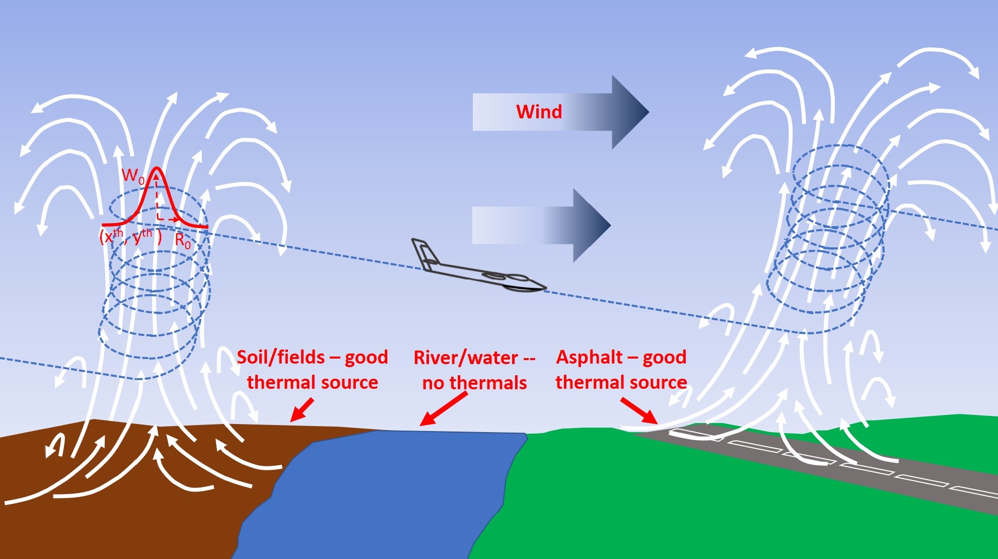
Figure 1: Thermals and their bell-shaped lift model (in red).

Researchers have proposed several approaches to enable autonomous thermalling for fixed-wing sUAVs [40, 41, 6, 16, 23, 33, 28]. Generally, they rely on various parameterized thermal models characterizing vertical air velocity distribution within a thermal. In order to successfully gain altitude in a thermal, a sUAV’s autopilot has to discover it, determine its parameters such as shape and lift distribution inside it, construct a trajectory that would exploit this lift, and exit at the right time. In this paper, we focus on autonomously identifying thermal parameters and using them to gain altitude. These processes are interdependent: thermal identification influences the choice of trajectory, which, in turn, determines what information will be collected about the thermal; both of these affect the decision to exit the thermal or stay in it.

Reinforcement learning (RL) [37], a family of techniques for resolving such exploration-exploitation tradeoffs, has been considered in the context of autonomous thermalling, but only in simulation studies [40, 41, 33, 28]. Its main practical drawback for this scenario is the episodic nature of classic RL algorithms. RL agents learn by executing sequences of actions (episodes) that are occasionally “reset”, teleporting the agent to its initial state. If the agent has access to an accurate resettable simulator of the environment, this is not an issue, and there have been attempts to build sufficiently detailed thermal models [33] for learning thermalling policies offline. However, to our knowledge, policies learned in this way have never tested on real sUAVs. Lacking a highly detailed simulator, in order to learn a policy for a specific thermal, a sUAV would need to make many attempts at entering the same thermal repeatedly in the real world, a luxury it doesn’t have. On the other hand, thermalling controllers tested live [5, 16] rely on simple, fixed strategies that, unlike RL-based ones, don’t take exploratory steps to gather information about a thermal. They were tested at high altitudes, where thermals are quite stable. However, below 200 meters, near the ground, thermals’ irregular shape makes the lack of exploration a notable drawback, as we show in this paper.

The main contribution of our work is framing and solving autonomous thermalling as partially observable Markov decision process (POMDP). A POMDP agent maintains a belief about possible world models (in our case — thermal models) and can explicitly predict how new information could affect its beliefs. This effectively allows the autopilot to build a simulator for a specific thermal in real time “on the fly”, and trade off information gathering to refine it versus exploiting the already available knowledge to gain height. We propose a fast approximate algorithm tailored to this scenario that runs in real time on Pixhawk, a common autopilot hardware that has a 32-bit ARM processor with only 168MHz clock speed and 256KB RAM. On sUAVs with a more powerful companion computer such as Raspberry Pi 3 onboard, our approach allows for thermalling policy generation with a full-fledged POMDP solver. Alternatively, our setup can be viewed and solved as a model-based Bayesian reinforcement learning problem [21].

For evaluation, we added the proposed algorithm to ArduPlane [1], an open-source drone autopilot, and conducted a live comparison against ArduSoar, ArduPlane’s existing soaring controller. This experiment comprised 14 missions, in which two RC sailplanes running each of the two thermalling algorithms onboard flew simultaneously in weak turbulent windy thermals at altitudes below 200 meters. Our controller significantly outperformed ArduSoar in flight duration in 11 flights out of 14, showing that its unconventional thermalling trajectories let it take advantage of the slightest updrafts even when running on very low-power hardware.

II Background

Thermals and sailplanes. Thermals are rising plumes of air that originate above areas of the ground that give up previously accumulated heat during certain parts of the day (Figure 1). They tend to occur in at least partly sunny weather several hours after sunrise above darker-colored terrain such as fields or roads and above buildings, but occasionally also appear where there are no obvious features on the Earth’s surface. As the warm air rises, it coalesces into a “column”, cools off with altitude and eventually starts sinking around the column’s fringes. As any conceptual model, this representation of a thermal is idealized. In reality, thermals can be turbulent and irregularly shaped, especially at altitudes up to 300m.

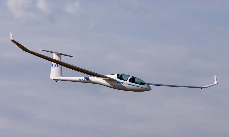
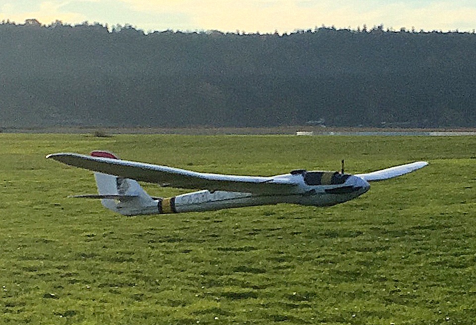
Figure 2: A full-size DG1000 sailplane (left, photo credit: Paul Hailday) and Radian Pro remote-controllable model sailplane that serves as our sUAV platform (right).

Thermal updrafts are used by birds [3] and by human pilots flying sailplanes. Sailplanes (Figure 2, left), colloquially also called gliders, are a type of fixed-winged aircraft optimized for unpowered flight, although some do have a limited-run motor. To test our algorithms, we use a Radian Pro sailplane sUAV (Figure 2, right) controllable by a human from the ground.

Thermalling strategies depend on the distribution of lift within a thermal. Much of autonomous thermalling literature, as well as human pilots’ intuition, relies on the bell-shaped model of lift in the horizontal cross-section of a thermal at a given altitude [41]. It assumes thermals to be approximately round, with vertical air velocity $w(x,y)$ being largest near the center and monotonically getting smaller towards the fringes:

$$w(x,y)=W_{0}e^{-\frac{(x-x^{th})^{2}+(y-y^{th})^{2}}{R_{0}^{2}}}$$ (1)

Here, $(x^{th},y^{th})$ is the position of the thermal center at a given altitude, $W_{0}$ is vertical air velocity, in m/s, at the center, and $R_{0}$ can be interpreted as the thermal’s radius (Figure 1, in red). Note that a thermal’s lift doesn’t disappear entirely more that $R_{0}$ meters from its center. In spite of its simplicity, we use this model in our controller for its low computational cost.

MDPs and POMDPs. Settings where an agent has to optimize its course of action are modeled as Markov Decision Processes (MDP). An MDP is a tuple $\langle\mathcal{S},\mathcal{A},\mathcal{T},\mathcal{R},s_{0}\rangle$ where $\mathcal{S}$ is the set of possible joint agent/environment states, $\mathcal{A}$ is the set of actions available to the agent, $\mathcal{T}:\mathcal{S}\times\mathcal{A}\times\mathcal{S}\rightarrow[0,1]$ is a transition function specifying the probability that executing action $a$ in state $s$ will change the state to $s^{\prime}$, $\mathcal{R}:\mathcal{S}\times\mathcal{A}\times\mathcal{S}\rightarrow\mathbb{R}$ is a reward function specifying the agent’s reward for such a transition, and $s_{0}$ is the start state. An MDP agent is assumed to know the current state exactly. An optimal MDP solution is a mapping $\pi:\mathcal{S}\rightarrow\mathcal{A}$ called policy that dominates all other policies under the expected reward value starting at $s_{0}$:

$$V^{\pi}(s_{0})=E_{\mathcal{T}^{\pi}}\left[\sum^{\infty}_{i=0}\gamma^{i}\mathcal{R}(S_{i},A^{\pi}_{i},S_{i+1})\biggr{\rvert}S_{0}=s_{0}\right]$$ (2)

Here, $S_{i}$ and $A^{\pi}_{i}$ are random variables for the agent’s state $i$ steps into the future and the action chosen by $\pi$ in that state, under trajectory distribution $\mathcal{T}^{\pi}$ induced by $\pi$ from $s_{0}$.

If the agent doesn’t have full state knowledge but has access to noisy state observations (as in this paper’s setting), it is in a partially observable MDP (POMDP) setting [8]. A POMDP is a tuple $\langle\mathcal{S},\mathcal{A},\mathcal{T},\mathcal{R},\mathcal{O},\mathcal{Z},b_{0}\rangle$, where $\mathcal{S},\mathcal{A},\mathcal{T}$, and $\mathcal{R}$ are as in the MDP definition, $\mathcal{O}$ is the observation space of possible clues about the true state, and $\mathcal{Z}:\mathcal{A}\times\mathcal{S}\times\mathcal{O}\rightarrow[0,1]$ describes the probabilities of these observations for different states $s^{\prime}$ where the agent may end up after executing action $a$. Since a POMDP agent doesn’t know the world state, it maintains a belief — a state probability distribution given the observations received so far. Initially, this distribution is a just a prior $b_{0}:\mathcal{S}\rightarrow[0,1]$; the agent updates it using the Bayes rule. POMDP policies are belief-based and have the form $\pi:\mathcal{B}\rightarrow\mathcal{A}$, where $\mathcal{B}$ is the belief space. The optimization criterion amounts to finding a policy that maximizes

$$V^{\pi}(b_{0})=\sum_{s}b_{0}(s)V^{\pi}(s)$$ (3)

where $V^{\pi}(s)$ comes from Equation 2. For a known initial belief state $b_{0}$, general POMDPs can be solved with different degrees of optimality using methods from the point-based family [32] or variants of the POMCP algorithm [35].

Extended Kalman filter. Since a POMDP agent’s action choice depends on its belief, efficient belief updates are crucial. For Gaussian beliefs, the Bayesian update can be performed very fast using various Kalman filters. In the POMDP notation, under stationary transition and observation functions, the original Kalman filter (KF) [25] assumes $\mathcal{T}(s,a,s^{\prime})=\mathcal{N}(s^{\prime}|f(s,a),Q)$ and $\mathcal{Z}(a,s^{\prime},o)=\mathcal{N}(o|h(a,s^{\prime}),R)$, where $\mathcal{N}$ denotes a Gaussian, $Q$ and $R$ are process and observation noise covariance matrices, and transition and observation transformations $f(s,a)$ and $h(a,s^{\prime})$ are linear in state and action features. If beliefs are Gaussian but$f(s,a)$ and $h(s^{\prime},a)$ are non-linear, as in our scenario, they can be linearized locally, giving rise to the extended Kalman filter (EKF).

Concretely, suppose that for belief $b=\mathcal{N}(.|\vec{\mu},\Sigma)$, the agent takes action $a$, gets observation $o$, and wants to compute its new belief $b^{\prime}=\mathcal{N}(.|\vec{\mu}^{\prime},\Sigma^{\prime})$. First, we linearize the transition $f(s,a)$ about the current belief by computing the Jacobian

$$F=\frac{\partial f}{\partial\vec{\mu}}\biggr{\rvert}_{\vec{\mu}}$$ (4)

and a new belief estimate not yet adjusted for observation $o$:

$$\vec{\underline{\mu}}^{\prime}=f(\vec{\mu},a)\ \ \ \ \ \ \ \underline{\Sigma}^{\prime}=F\Sigma F^{\intercal}+Q$$ (5)

Next, we linearize $h(a,s^{\prime})$ around this uncorrected belief by producing the Jacobian

$$H=\frac{\partial h}{\partial\vec{\mu}}\biggr{\rvert}_{a,\vec{\underline{\mu}}^{\prime}}$$ (6)

and compute the approximate Kalman gain

$$K=\underline{\Sigma}^{\prime}H^{\intercal}(H\underline{\Sigma}^{\prime}H^{\intercal}+R)^{-1}$$ (7)

Finally, we correct our intermediate belief for observations:

$$\vec{\mu}^{\prime}=\vec{\underline{\mu}}^{\prime}+K(\vec{o}-h(a,\vec{\underline{\mu}}^{\prime}))\ \ \ \ \ \ \ \ \ \Sigma^{\prime}=(I-KH)\underline{\Sigma}^{\prime}\\$$ (8)

There are other filters for belief tracking in systems with non-linear dynamics, including unscented Kalman filter (UKF) [24] and particle filter (PF) [29]. We choose EKF for its balance of approximation quality and low computational requirements.

III Autonomous Thermalling as a POMDP

Our formalization of autonomous thermalling is based on the fact that within a thermal, a sUAV’s probability of gaining altitude and altitude gain itself depend on the lift distribution (in our case, given by Equation 1). Thus, in the MDP/POMDP terminology, the lift distribution model determines the transition and reward functions $\mathcal{T}$ and $\mathcal{R}$. Since Equation 1’s parameters are initially unknown, neither are $\mathcal{T}$ and $\mathcal{R}$. However, the autopilot can keep track of a belief $b$ over model parameters $x^{th},y^{th},W_{0}$, and $R_{0}$ as it is receiving a stream of variometer data, making POMDP a natural choice for this scenario.

The belief $b$ characterizes the autopilot’s uncertainty about the thermal’s position, size, and strength. Based on its current belief, at any time the autopilot can simulate observations it might get from measuring lift strength at different locations, and estimate how this knowledge is expected to reduce its thermal model uncertainty. This simulation can also help assess the expected net altitude gain from following various trajectories. Thus, the autopilot can deliberately select trajectories that reduce its model uncertainty in addition to providing lift. The ability to explicitly plan environment exploration is missing both from all thermalling controllers proposed so far, including those that use RL (see the Related Work section). As hypothesized by Allen and Lin [6], Edwards [16], and Tabor et al. [38], and as demonstrated in our experiments, this ability is important, especially for thermalling in difficult conditions.

The POMDP we formulate models the decision-making process once the sailplane is in a thermal. Note that gaining altitude with the help of an updraft also involves thermal detection and timely exit. These are beyond the paper’s scope; we rely on Tabor et al. [38]’s mechanisms to implement them.

Practicalities, assumptions, and mode of operation

First we identify our scenario’s aspects that may violate POMDPs’ assumptions, and adapt POMDPs to them.

Thermalling as model predictive control. POMDPs assume the environment to be stationary, i.e., governed by unchanging $\mathcal{T}$ and $\mathcal{R}$. Viewing thermalling in this way would require modeling thermal evolution, which is computationally expensive, error-prone, and itself involves assumptions. Instead, as is common for such scenarios, we view it as a model predictive control (MPC) problem [20]. Our controller gets invoked with a fixed frequency of $>1$Hz, solves the POMDP below approximately to choose an action for the current belief, and the process repeats at the next time step.

Modelling assumptions. The policy quality of our controller depends on the validity of the following assumptions:

• Assumption 1. The thermal changes with time no faster than on the order of tens of seconds, and is approximately the same within a few meters of vertical distance. This ensures that the world model used by the controller to choose the next action isn’t too different from the world where this action will be executed. Recall that Equation 1 applies to a given altitude, and as the sUAV thermals, its altitude changes. The assumption is that, locally, the thermal doesn’t change with altitude too much.

• Assumption 2. The thermal doesn’t move w.r.t. the surrounding air. The air mass containing both the thermal and the sUAV may move w.r.t. the ground due to wind. We effectively assume that the thermal moves at the wind velocity. While this assumption isn’t strictly true for thermals [39], it is common in the autonomous thermalling literature, and its violation doesn’t seriously affect our controller, which recomputes the policy frequently.

• Assumption 3. The sUAV is flying at a constant airspeed, and the thermalling controller can’t change the sUAV’s pitch angle at will. During thermalling, pitch angle control is necessary only for maintaining airspeed and executing coordinated turns, which can be done by the lower levels of the autopilot. If the thermalling controller could change pitch directly, it might attempt to “cheat” by using it to convert kinetic energy into potential to gain altitude, instead of exploiting thermal lift to do so.

• Assumption 4. The thermal has no effect on the sUAV’s horizontal displacement. This holds for the model in Equation 1 because that model disregards turbulence.

A note on reference frames. Wind complicates some computations related to sUAV’s real-world state, because the locations of important observations such as lift strength are given in Earth’s reference frame, in terms of GPS coordinates, whereas the sUAV drifts with the wind. The autopilot maintains a wind vector estimate and uses it to translate GPS locations to the air mass’s reference frame [23, 38].

To make wind correction unnecessary, our POMDP model reasons entirely in the reference frame of the air mass. Due to Assumption 2 above, in this frame sUAV’s air velocity fully accounts for the thermal’s displacement w.r.t. the sUAV. When solving the POMDP involves simulating observations, their locations are generated directly in this reference frame too.

POMDP Formulation

The components of the thermalling POMDP are as follows:

State space $\mathcal{S}$ consists of vectors $(s^{u},s^{th})$ describing the joint state of the sUAV ($s^{u}$) and the thermal ($s^{th}$). In particular, $s^{u}=(\vec{p}^{u},v,\psi,\phi,\dot{\phi},h)$ and $s^{th}=(\vec{p}^{th},W_{0},R_{0})$, where $\vec{p}^{u}$ gives the 2-D location, in meters, of the sUAV w.r.t. an arbitrary but fixed origin of the air mass coordinate system, $v$ is sUAV’s airspeed in m/s, $\psi$ is its heading – the angle between north and the direction in which it is flying, $\phi$ is its bank angle, $\dot{\phi}$ is its rate of roll, and $h$ is its altitude w.r.t. the mean sea level (MSL). The thermal state vector consists of $\vec{p}^{th}$ $=(x^{th},y^{th})$ – the 2-D position of the thermal model center relative to the sUAV position, $W_{0}$ – the vertical lift in m/s at the thermal center and $R_{0}$ – the thermal radius (Figure 1).

Wind vector $\vec{w}$ and pitch angle are notably missing from the state space definition due to Assumptions 2 and 3.

Action space $\mathcal{A}$ is a set of arc-like sUAV trajectory segments originating at the sUAV’s current position, parametrized by duration $T_{\mathcal{A}}$ common to all actions and indexed by a set of bank angles $\{\phi_{1},\ldots,\phi_{n}\}$. Each trajectory corresponds to a coordinated turn at bank angle $\phi_{i}$ for $T_{\mathcal{A}}$ seconds. It is not exactly an arc, because attaining bank angle $\phi_{i}$ takes time dependent on sUAV’s roll rate $\dot{\phi}$ and current bank angle $\phi$.

Transition function $\mathcal{T}$ gives the probability of the joint system state $s^{\prime}$ after executing action $a$ in state $(s^{u},s^{th})$. Under Assumptions 2 and 4, $\mathcal{T}$ is described by the sUAV’s dynamics and Gaussian process noise:

$$\mathcal{T}(s,a,s^{\prime})=\mathcal{N}(s^{\prime}|f_{T_{\mathcal{A}}}(s,a),Q)$$ (9)

Here, $f_{T_{\mathcal{A}}}$ captures the sUAV’s dynamics, $Q$ is the process noise covariance matrix, and $\mathcal{T}$ satisfies a crucial property: $\mathcal{T}$ does not modify thermal parameters $W_{0}$, $R_{0}$, and thermal center $\vec{p}^{th}$ w.r.t. sUAV’s position $\vec{p}^{u}$ in $s$. Intuitively, thermal doesn’t change just because the sUAV moves. The change in the thermal center position is purely due to sUAV’s motion and the fact that the thermal’s position is relative to sUAV’s.

Reward function $\mathcal{R}$ for states $s$ and $s^{\prime}$ is $(h_{s}-h_{s^{\prime}})$, the resulting change in altitude. This definition relies on Assumption 3. Without it, thermalling controller could gain altitude by manipulating pitch, not by exploiting thermal lift.

Observation set $\mathcal{O}$ consists of the possible sets of sensor readings of airspeed sensor, GPS, and barometer readings that the sUAV might receive while executing an action $a$.

Observation function $\mathcal{Z}$ assigning probabilies $\mathcal{Z}(a,s^{\prime},o)$ to various observation sets $o$ is governed by action $a$’s trajectory and Gaussian process noise covariance matrix $R$. Each of sUAV’s sensors operates at some frequency $\xi$. During $a$’s execution, this sensor generates a sequence of datapoints of length $\xi T_{\mathcal{A}}$, each sampled from a 0-mean Gaussian noise around the corresponding intermediate point on $a$’s trajectory. The probability of a set of sensor data sequences produced during $a$’s execution is the product of corresponding Gaussians.

Initial belief $b_{0}$ is given by a product of two Gaussians:

$$b_{0}(s)=b_{0}(s^{u})b_{0}(s^{th})=\mathcal{N}(s^{u}|s^{u}_{0},\Sigma_{0}^{u})\mathcal{N}(s^{th}|s^{th}_{0},\Sigma_{0}^{th}),$$

where $s^{u}_{0}$ has $\vec{p}_{0}^{u}=(0,0)$ for mathematical simplicity, because sUAV’s position is w.r.t. the air mass and for POMDP’s purposes isn’t tied to any absolute location, and $s^{u}_{0}$’s other components are sUAV’s current airspeed, roll, etc. $s^{th}_{0}$ is initialized with estimates of thermals generally encountered in the area of operations. $\Sigma_{0}^{u}$ and $\Sigma_{0}^{th}$ are diagonal matrices.

Keeping the belief components for sUAV and thermal state separate is convenient for computational reasons. The sUAV state observations are heavily filtered sensor signals, so in practice sUAV’s state can be treated as known. At the same time, thermal state belief, especially the initial belief $b^{th}_{0}$, has a lot of uncertainty and will benefit from a full belief update.

Belief updates are a central factor determining the computational cost of solving a POMDP. Our primary motivation for defining the initial belief $b_{0}$ to be Gaussian, in spite of possible inaccuracies, is that we can repeatedly use the EKF defined in Equations 4-8 to update $b_{0}$ with new observations and get a Gaussian posterior $b^{\prime}$ at every step:

$$b^{\prime}=\mbox{EKF\_update}(b_{0},a,\vec{o})$$ (10)

The EKF_update routine implicitly uses transition and observation functions $\mathcal{T}$ and $\mathcal{Z}$ from the POMDP’s definition.

IV The Algorithm

1 Input: POMDP $\langle{\cal S},{\cal A},{\cal T},{\cal R},{\cal O},{\cal Z},b_{0}\rangle$, $N$ – number of thermal state belief samples, $T^{\mbox{exploit}}_{\mathcal{A}}$ – planning horizon for exploitation mode, $T^{\mbox{explore}}_{\mathcal{A}}$ – planning horizon for exploration mode, $\Delta t$ – action trajectory time resolution, THERMAL_CONFIDENCE_THRES – thermal state confidence threshold

2

3$b_{0}=\mathcal{N}(s^{u}_{0},\Sigma_{0}^{u})\mathcal{N}(s^{th}_{0},\Sigma_{0}^{th})\leftarrow$ current belief

4  

5 if $tr(\Sigma_{0}^{th})<\mbox{THERMAL\_CONFIDENCE\_THRES}$ then

6       Go to EXPLOIT

7else

8       Go to EXPLORE

9 end if

10 

11 EXPLORE begin

12       foreach $a\in\mathcal{A}$ do

13             $\mbox{Traj}_{a}\leftarrow\mbox{\text@underline{SimActionTraj}}(s^{u}_{0},\phi_{a},\Delta t,T^{\mbox{explore}}_{\mathcal{A}})$

14             foreach $i=1\ldots N$ do

15                   $s^{th}_{i}\leftarrow\mbox{\text@underline{SampleThermalState}}(b_{0})$

16                   foreach $t=1\ldots\mbox{Traj}_{a}.\mbox{Length}$ do

17                         $\vec{o}_{a,i,t}\leftarrow\mbox{\text@underline{SimObservation}}(\mbox{Traj}_{a}[t],s^{th}_{i})$

18                         $b_{a,i,t}\leftarrow\mbox{EKF\_update}(b_{a,i,t-1},a_{[t-1,t]},\vec{o}_{a,i,t})$

19                        

20                   end foreach

21                  $\Sigma^{th}_{a,i}\leftarrow\mbox{covariance of }b_{a,i,Traj_{a}.\mbox{Length}}$

22                  

23             end foreach

24            $\mbox{Uncertainty}_{a}\leftarrow\frac{\sum_{i=1}^{N}tr(\Sigma^{th}_{a,i})}{N}$

25            

26       end foreach

27      $a^{*}\leftarrow\mbox{argmin}_{a\in\mathcal{A}}\mbox{Uncertainty}_{a}$

28       Return $a^{*}$

29      

30 end

31

32 

33 EXPLOIT begin

34       foreach $a\in\mathcal{A}$ do

35             $\mbox{Traj}_{a}\leftarrow\mbox{\text@underline{SimActionTraj}}(s^{u}_{0},\phi_{a},\Delta t,T^{\mbox{exploit}}_{\mathcal{A}})$

36             foreach $i=1\ldots N$ do

37                   $s^{th}_{i}\leftarrow\mbox{\text@underline{SampleThermalState}}(b_{0})$

38                   foreach $t=1\ldots\mbox{Traj}_{a}.\mbox{Length}$ do

39                         $w_{a,i,t}\leftarrow\mbox{\text@underline{SimLift}}(\mbox{Traj}_{a}[t],s^{th}_{i})$

40                        

41                   end foreach

42                  $\mbox{AltGain}_{a,i}\leftarrow\sum^{\mbox{Traj}_{a}.\mbox{Length}}_{t=1}w_{a,i,t}\Delta t$

43                  

44             end foreach

45            $\mbox{ExpAltGain}_{a}\leftarrow\frac{\sum_{i=1}^{N}\mbox{AltGain}_{a,i}}{N}$

46            

47       end foreach

48      $a^{*}\leftarrow\mbox{argmax}_{a\in\mathcal{A}}\mbox{ExpAltGain}_{a}$

49       Return $a^{*}$

50      

51 end

52

Algorithm 1 POMDSoar

Although using EKF-based belief updates reduces the computational cost of solving a POMDP, solving an EKF-based POMDP near-optimally on common low-power flight controllers such as APM and Pixhawk is still much too expensive. The algorithm we present, POMDSoar (Algorithm 1), makes several fairly drastic approximations in order to be solve the POMDP model. While they undoubtedly lead to sacrifices in solution quality, POMDSoar still retains a controller’s ability to explore in a (myopically) guided way, which, we claim, gives it advantage in messy thermals at low altitudes. This section presents a high-level description of POMDSoar, while further details about its tradeoffs and implementation are contained in the Appendix.

To further reduce belief update cost, POMDSoar always uses the belief mean as the estimate of the sUAV state; see, e.g., line 1 of Algorithm 1. For the thermal part of the state, however, it uses the full belief over that part. For a Gaussian, it is natural to take covariance trace as a measure of uncertainty, and this is what POMDSoar does (lines 1, 1).

Conceptually, POMDSoar is split into two parts: exploration and exploitation. Whenever it is invoked, it first analyzes the covariance of the controller’s current belief about the thermal state (line 1). If its trace is below a given threshold — an input parameter — POMDSoar chooses an action aimed at exploiting the current belief. Otherwise, it tries to reduce belief uncertainty by doing exploration. In effect, POMDSoar switches between two approximations of the POMDP reward function $\mathcal{R}$, an exploration- and a lift-oriented one.

In either mode, POMDSoar performs similar calculations. Its action set is a set of arcs parametrized by discrete roll angles, e.g. -45, -30, -15, 0, 15, 30, and 45 degrees. For each of them it computes the sequence of points that would result from executing a coordinated turn at that roll angle for $T^{\mbox{explore}}_{\mathcal{A}}$ or $T^{\mbox{exploit}}_{\mathcal{A}}$ seconds (lines 1, 1). See the Implementation Details section for more information about this computation.

Then, POMDSoar samples $N$ thermal states from the current belief and for each of these “imaginary thermals” simulates the reward of executing each of the above action trajectories in the presence of this thermal. In explore mode, action reward is the reduction in belief uncertainty, so at each of the trajectory points POMDSoar generates a hypothetical observation and uses it in a sequence of imaginary belief updates (line 1). The trace of the last resulting belief measures thermal belief uncertainty after the action’s hypothetical execution. For execution in the real world, POMDSoar chooses the action that minimizes this uncertainty.

In the exploit mode, at each generated point of each action trajectory, POMDSoar measures hypothetical lift (line 1) instead of generating observations, and then integrates the lift along the trajectory to estimate altitude gain (line 1). The action with the maximum altitude gain estimate ”wins”.

POMDSoar’s performance in practice critically relies on the match between the actual turn trajectory (a sequence of 2-D locations) the sUAV will follow for a commanded bank angle and the turn trajectory predicted by our controller for this bank angle and used by POMDSoar during planning. Our controller’s trajectory prediction model is in the Appendix. It uses several airframe type-specific parameters that had to be fitted to data gathered by entering the sUAV into turns at various bank angles. The model achieves a difference of $<1$m between predicted and actual trajectories. Figure 3 shows the match between the model-predicted and actual bank and aileron deflection angle evolutions for several roll commands.

Our POMDSoar implementation is available at https://github.com/Microsoft/Frigatebird. It is in C++ and is based on ArduPlane 3.8.2, an open-source autopilot for fixed-wing drones [1] that has Tabor et al. [38]’s ArduSoar controller built in. We reused the parts of it that were conceptually common between ArduSoar and POMDSoar, including the thermal tracking EKF and thermal entry/exit logic. ArduSoar and POMDSoar implementations differ only in how they use the EKF to choose the sUAV’s next action. Running POMDSoar onboard a sUAV requires picking input parameters (Algorithm 1, line 1) that result in reasonable-quality solutions within the short ($<1$s) time between controller invocations on the flight controller hardware. All parameters values from our experiments are available in a .param file together with POMDSoar’s implementation.

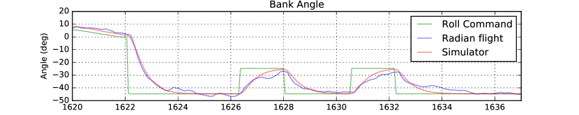
(a) Bank angle

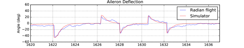
(b) Aileron deflection angle

Figure 3: Comparison between actual flight data and its predictions by the model used in POMDSoar for the same input roll commands.

V Related Work

While our approach can be regarded as solving an POMDP, it is also an instance of Bayesian reinforcement learning (BRL) [18, 21]. In BRL, the agent starts with a prior distribution over model dynamics $\mathcal{T}$ and $\mathcal{R}$, and maintains a posterior over them as it gets observations. Viewing $\mathcal{T}$ and $\mathcal{R}$ as part of the augmented state space $\mathcal{S}^{\prime}=\mathcal{S}\times\mathcal{T}\times\mathcal{R}$ reveals that BRL is equivalent to a special POMDP called Bayes-adaptive MDP (BAMDP) [15], which POMDSoar ends up solving. Nonetheless, due to the computational constraints of our platform, POMDSoar is very different from existing POMDP and BRL solvers such as POMCP [35] and BAMCP [22]. However, BRL-induced POMDPs with belief tracking using EKF were studied by Slade et al. [36], and the idea of separating uncertainty reduction from knowledge exploitation for approximate BRL is similar to Dearden et al. [13].

There is vast literature on automatically exploiting thermals [40, 41, 6, 16, 23, 33, 28], orographic lift [26, 19], wind gusts [27], wind fields [31], and wind gradients [30, 9], as well as on planning flight paths to extend fixed-wing sUAV endurance and range [17, 31, 10, 11, 28, 14]. Soaring patterns have also been studied for birds [3]. Since our paper focuses exclusively on thermalling, here we survey papers from this subarea.

In an early autonomous thermalling work, Wharington et al [40, 41] used RL [37] in simulation to learn a thermalling strategy under several simplifying assumptions. Reddy et al. [33] also used RL but removed some of Wharington and Herszberg [41]’s simplifications. In particular, they built a far more detailed thermal model that reflects updrafts’ messy, turbulent nature. However, neither of these techniques have been deployed on real UAVs so far, and how this could be done is conceptually non-obvious. These works’ version of RL would require executing many trials in the real world in order to learn a thermalling strategy for a given situation, including the ability to restart a trajectory at will — a luxury unavailable to real-world sUAVs. Given the wide variability in atmospheric conditions, it is also unclear whether this method can be successfully used to learn a policy offline for subsequent deployment onboard a sUAV. Our POMDP model circumvents these challenges facing classical RL in the autonomous soaring scenario, since the former allows sampling trajectories during flight on the flight controller’s hardware running a data-driven simulator built on the go. However, incorporating Reddy et al. [33]’s elaborate thermal model into a POMDP-based controller could yield even more potent thermalling strategies.

Allen and Lin [6] were the first to conduct an extensive live evaluation of an automatic thermalling technique. They employed a form of Reichmann rules [6, 34] — a set of heuristics employed for thermal centering by human pilots — to collect data for learning thermal location and radius in flight. Edwards [16] mitigated this approach’s potential issue with biased thermal parameter estimates. In a live flight test conducted primarily at altitudes over 700m, the resulting method along with inter-thermal speed optimization kept a sailplane airborne for 5.3 hours, the record for automatic soaring so far, with thermal centering running on a laptop on the ground. It is not clear whether it is possible to implement it as part of a fully autonomous autopilot on such a computationally constrained device as a Pixhawk, and how such an implementation, if realistic, would perform in less regular low-altitude thermalling conditions. Another controller based on Reichmann rules was introduced by Andersson et al. [7]. Daugherty and Langelaan [12] improved on it by using a Savitzky-Golai filter to estimate total specific energy and its derivatives, which reduced the estimation lag compared to Andersson et al. [7] and allowed latching onto smaller thermals in simulation. Andersson et al. [7]’s controller itself, like those of Edwards [16] and Allen and Lin [6], was evaluated on a real sUAV and did well at altitudes over 400m AGL, but relative live performance of all these controllers is unknown.

Last but not least, our live study compares POMDSoar against ArduSoar [38], the thermalling controller of a popular open-source autopilot for fixed-wing sUAVs called ArduPlane [1]. ArduSoar’s implementation of thermal-tracking EKF and thermal entry/exit logic is shared with POMDSoar. When ArduSoar detects a thermal, it starts circling at a fixed radius around the EKF’s thermal position estimate mean. ArduSoar’s thermal tracking was inspired by Hazard [23]’s work, which used a UKF instead of EKF for this purpose and evaluated a number of fixed thermalling trajectories in simulation.

Thus, several aspects distinguish our work from prior art. On the theoretic level, we frame thermalling as a POMDP, which allows principled analysis and practical onboard solutions. We also conduct the first live side-by-side evaluation of two thermalling controllers. Last but not least, this evaluation is done in an easily replicable experimental setup.

VI Empirical Evaluation

Our empirical evaluation aimed at comparing POMDSoar’s performance as part of an end-to-end sUAV autopilot to a publicly available thermalling controller for sUAVs, ArduSoar, in challenging real-life thermalling conditions. We did this via side-by-side live testing of the two soaring controllers. The choice of ArduSoar as a baseline is motivated by several considerations. First, despite its simplicity, it performs well at higher altitudes. Second, it incorporates central ideas from several other strong works, including Allen and Lin [6], Edwards [16], and Hazard [23]. Third, the availability of source code, documentation, parameters, and hardware for it eliminates from our experiments potential performance differences due to hardware capabilities, implementation tricks, or mistuning.

A field study of a thermalling controller is complicated by exogenous factors such as weather, so before presenting the results we elaborate on the evaluation methodology.

Equipment. We used two identical off-the-shelf Radian Pro remote-controllable sailplanes as sUAV airframes. They are made of styrofoam, have a 2m wingspan, 1.15m length, and carry a motor that can run for a limited duration. To enable them to fly autonomously, we reproduced the setup from Tabor et al. [38], installing on each a 3DR Pixhawk flight controller (32-bit 168MHz ARM processor, 256KB RAM, 2MB flash memory), a GPS, and other peripherals, as shown in Figure 4. A human operator could take over control at will using an X9D+ remote controller. All onboard electronics and the motor was powered by a single 3-cell 1300 mAh LiPo battery.

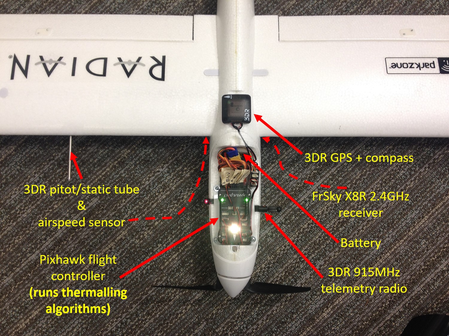
Figure 4: Radian Pro sUAV’s electronic equipment

Software. Both Radian Pros ran the ArduPlane autopilot modified to include POMDSoar, as described in the Implementation Details section of the Appendix. During each flight, POMDSoar was enabled on one Radian Pro, and ArduSoar was enabled on the other. We used Mission Planner v1.3.49 [2] as ground control station (GCS) software to monitor flight telemetry in real time. ArduPlane was tuned separately on each airframe using a standard procedure [1]. The parameters not affected by tuning were copied from Tabor et al. [38]’s, setup, including the target airspeed of 9 m/s. The airspeed sensors were recalibrated before every flight.

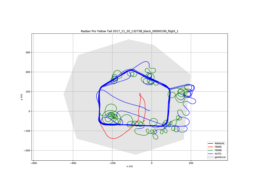
(a) The Field test site and POMDSoar’s typical flight path at it.

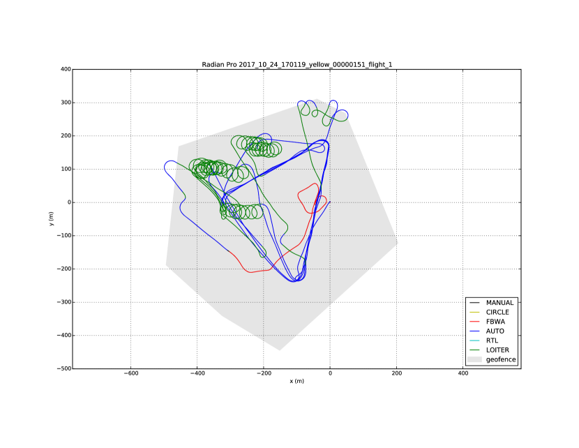
(b) The Valley test site and ArduSoar’s typical flight path at it.

Figure 5: The Field and Valley test site layout and typical mission flight paths due to POMDSoar and ArduSoar. When not thermalling (AUTO mode), the sUAVs follow a fixed sequence of waypoints, resulting in a pentagon-shaped path at the Field site and a triangle-shaped one at the Valley. During thermalling, the sUAVs are allowed to deviate from this path anywhere within the geofenced region shown in grey. In the thermalling mode (FBWB for POMDSoar, LOITER for ArduSoar, green sections of the paths), POMDSoar does a lot of exloration, yielding irregularly-shaped meandering trajectories. ArduSoar, due to a more rigid thermalling policy, yields spiral-shaped paths that result in little exploration. Both controllers are forced to give up thermalling and switch to AUTO mode if the sUAV breaches the geofence.

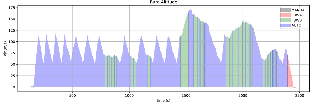
(a) Altitude plot for a typical thermalling flight.

(b) Altitude plot for a typical baseline measurement flight.

Figure 6: Altitude vs. time plots for thermalling and baseline flights illustrating the mission profile. After being hand-tossed into the air in AUTO mode, each Radian automatically started its motor and climbed to the altitude given by SOAR_ALT_CUTOFF. At that altitude, it would shut down the motor and glide down, still in AUTO mode, until it either reached SOAR_ALT_MIN or detected a thermal. In the latter case, it would abandon waypoint following and enter a thermalling mode (FBWB for POMDSoar, LOITER for ArduSoar) until it gained altitude up to SOAR_ALT_MAX, descended to SOAR_ALT_MIN if the thermalling attempt was unsuccessful, or hit the geofence. In all these cases, the AUTO mode would engage automatically, forcing the sUAV to give up thermalling, guiding it to the next waypoint, and turning on the motor if necessary to climb from SOAR_ALT_MIN to SOAR_ALT_CUTOFF. For Field and Valley test sites, SOAR_ALT_MIN is 50m and 30m, SOAR_ALT_CUTOFF is 110m and 130m, and SOAR_ALT_MAX is 160m and 180m, respectively.

Figure 7: Relative gains in flight time over the baseline (Equation 11) for POMDSoar and ArduSoar across 14 flights at the Valley(V) and Field(F) test sites. POMDSoar outpeformed ArduSoar overall, yielding higher gains in 11 flights, losing in 1, and ending 2 in a draw.

Location. Flights took place at two test sites denoted Valley and Field located in the Northwestern USA around 47.6°N, 122°W approximately 16km apart, each $\approx 700$m in diameter. Figure 5 shows their layout, waypoint tracks, and geofences.

Flight conditions. All flights for this experiment took place between October 2017 and January 2018. Regional weather during this season is generally poor for thermalling, with low daily temperatures and their amplitudes (a major factor for thermal existence and strength), nearly constant cloud cover, and frequent gusty winds and rain. All flights were carried out in dry but at best partly cloudy weather, at temperatures $\leq 14$°C and daily temperature amplitudes $\leq 9$°C. All took place in predominant winds between 2 and 9 m/s; in $\approx 25$% of the missions, the wind was around 7 m/s – 78% of our sUAVs’ 9 m/s airspeed during thermalling and off-motor glides.

Flight constraints. Due to regulations, all flights were geofenced as shown in Figure 5 and restricted to low altitudes: 180m AGL at the Valley and 160m AGL at the Field site. To avoid collision with ground obstacles, the minimum autonomous flight altitude was 30m and 50m AGL, respectively.

Mission profile. Each mission consisted in two Radian Pros, one using POMDSoar and another using ArduSoar as thermalling controller, taking off within seconds of each other and repeatedly flying the same set of waypoints at a given test site counterclockwise from the Home location as long as their batteries lasted, deviating from this path only during thermal encounters. Figure 6(a) explains the mission pattern.

Each flight was fully autonomous until either the sUAV’s battery voltage, as reported in the telemetry, fell below 3.3V/cell for 10s during motor-off glide, or for 10s was insufficient to continue a motor-on climb. At that point, the mission was considered over. A human operator would put the sUAV into the Fly-By-Wire-A mode and land it.

Eliminating random factors. Live evaluation of a component as part of an end-to-end system is always affected by factors exogenous to the component. The Appendix details the measures we took to eliminate many of these factors, including the presence of non-thermal lift, potential systematic bias due to minor airframe and battery differences, and high outcome variance due to chance of finding thermals.

Performance measure. We compare POMDSoar and ArduSoar in terms of the relative increase in flight duration they provide. Namely, for a flight at test site $S$ where controller $C^{th}$ ran on airframe $A$ and used battery $B$, we compute

$$\textit{RelTimeGain}_{A,B,S}(C^{th})=\frac{\textit{FlightTime}_{A,B,S}(C^{th})}{\textit{BaselineFlightTime}_{A,B,S}}$$ (11)

The $\textit{BaselineFlightTime}_{A,B,S}$ values are averages over durations of a series of separate flights in calm conditions with thermalling controllers turned off (see the Appendix).

Results

Our comparison is based on 14 two-sUAV thermalling flights performed in the above setup. Figure 7 shows the results. Importantly, they are primarily indicative of controllers’ advantages over each other, rather than each controller’s absolute potential to extend flight time, due to altitude and geofence restrictions that often forced sUAVs out of thermals, and the deliberate lack of a thermal finding strategy.

Qualitatively, as Figure 7 indicates, POMDSoar outpeformed ArduSoar in 11 out of 14 flights, and did as well in 2 of the remaining 3. Moreover, the flight time gains POMDSoar provides are appreciably larger compared to ArduSoar’s. The data in the “Effect of baseline correction” subsection of the Appendix adds more nuance. It shows that without baseline correction (Equation 11), the results look somewhat different, even though POMDSoar still wins in 11 flights.

These results agree with our hypothesis that in turbulent low-altitude thermals, POMDP-driven exploration and action selection are critical for taking advantage of whatever lift there is. Likely due to active exploration, POMDSoar’s trajectories can be much ”messier” than ArduSoar’s; see Figure 5.

VII Conclusion

This paper has presented a POMDP-based approach to autonomous thermalling. Viewing this scenario as a POMDP has allowed us to analyze it in a principled way, to identify the assumptions that make our approach feasible, and to show that this approach naturally makes deliberate environment exploration part of the thermalling strategy. This part is missing from prior work but is very important for successful thermalling in turbulent low-altitude conditions, as our experiment have demonstrated. We have presented a light-weight thermalling algorithm, POMDSoar, deployed it onboard a sUAV equipped with a computationally constrained Pixhawk flight controller, and conducted an extensive field study of its behavior. Our experimental setup is easily replicable and minimizes the effect of external factors on soaring controller evaluation. The study has shown that in challenging low-altitude thermals, POMDSoar outperforms the soaring controller included in ArduPlane, a popular open-source sUAV autopilot. Despite encouraging exploration, due to Pixhawk’s computational constraints POMDSoar makes many approximations. However, companion computers on larger sUAVs may be able to run a full-fledged POMDP solver in real time. Design and evaluation of a controller based on solving the thermalling POMDP near-optimally, e.g., using an approach similar to Slade et al. [36]’s, is a direction for future work.

Acknowledgements. We would like to thank Eric Horvitz, Chris Lovett, Shital Shah, Debadeepta Dey, Ashish Kapoor, Nicholas Lawrance, and Jen Jen Chung for thought-provoking discussions relevant to this work.

VIII APPENDIX

VIII-A Implementation Details

To make POMDSoar’s implementation configurable, we have added several parameters used by POMDSoar to ArduPlane’s SOAR_* parameter group. They have an effect only if thermalling functionality is turned on by setting the SOAR_ENABLE parameter to 1 [38]. The new SOAR_POMDP_ON parameter determines whether the sUAV  should use POMDSoar or ArduSoar for thermalling. Similar to ArduSoar adapting ArduPilot’s LOITER mode for thermalling, we implemented POMDSoar in Fly-By-Wire-B (FBWB) mode. This mode is similar to AUTO, but doesn’t try to follow waypoints. In particular, POMDSoar relies on the fact that ArduPlane in FBWB will control the pitch and yaw channel to execute a coordinted turn if a roll angle (POMDSoar’s output) is provided as input.

POMDSoar’s performance in practice critically relies on the match between the actual turn trajectory (a sequence of 2-D locations) the sUAV will follow for a commanded bank angle and the turn trajectory predicted by our controller for this bank angle and used by POMDSoar during planning. To predict the sequences of locations corresponding to different actions’ trajectories, our implementation uses differential Equations 12 through 15:

$$L_{p} =-\mathbf{K}_{d}\frac{\mathbf{C}_{lp}\dot{\phi}}{2v}$$ (12)

$$\ddot{\phi} =\frac{\mathbf{K}_{a}\delta_{a}-L_{p}}{I_{x}}$$ (13)

$$\dot{\psi} =\frac{g\tan\phi}{v}$$ (14)

$$\dot{\vec{p}^{u}} =\left(v\sin\psi,v\cos\psi\right)$$ (15)

The meanings of the variables and the constants in these equations, as well as the constants’ corresponding parameter names in ArduPlane and their values for Radian Pro airframes, are as follows:

• $\psi$ is the aircraft heading in radians,

• $\phi$ is the aircraft bank angle in radians,

• $L_{p}$ is the roll damping moment,

• $I_{x}$ is the moment of inertia about the aircraft roll axis. In ArduPlane, the corresponding parameter we have added is SOAR_I_MOMENT. For our Radian Pro sUAV, $I_{x}=0.00257482=m_{\mathrm{radian}}k^{2}$, where $m_{\mathrm{radian}}=1.2$kg is the measured mass of our modified Radian Pro and $k=0.05$ is estimated from the distribution of area in the lateral cross section.

• $v$ is airspeed in m/s.

• $\mathbf{C}_{lp}$ is the roll damping derivative. In ArduPlane, the corresponding new parameter is SOAR_ROLL_CLP. For a Radian Pro, $\mathbf{C}_{lp}=-\frac{1}{4}\frac{\pi AR}{\sqrt{\frac{AR^{2}}{4}+4}+2}=-1.12808704$, where $AR=11.8645073263$ is the wing aspect ratio calculated from dimensional measurements of the Radian Pro’s wing.

• $\mathbf{K}_{d}$ is a coefficient accounting for the wing span and other aerodynamic effects on roll damping. ArduPlane’s corresponding parameter is SOAR_K_ROLLDAMP. For a Radian Pro, $\mathbf{K}_{d}=0.41073588$.

• $\delta_{a}=f_{\phi_{\mathrm{PID}}}\left(\phi_{a}-\phi\right)$, the aileron deflection signal $\in[-1,1]$, where $f_{\phi_{\mathrm{PID}}}$ is ArduPlane’s roll channel PID controller function and $\phi_{a}$ is the commanded bank angle for the action.

• $\mathbf{K}_{a}$ is a coefficient accounting for the rolling forces due to aileron deflection. In ArduPlane, the respective parameter is SOAR_K_AILERON. For a Radian Pro, $\mathbf{K}_{a}=1.448331$.

• $g$ is the acceleration due to gravity.

Note that $L_{p}$ and $\delta_{a}$ depend on ArduPlane’s PID controller parameters, and $I_{x},\mathbf{C}_{lp},\mathbf{K}_{d},\mathbf{K}_{a}$ are specific to the airframe type. The latter constants need to fitted to data gathered by entering the sUAV into turns at various bank angles.

In order to predict a sequence of locations that constitute an action’s trajectory given the sUAV’s current state, our thermalling controller implementation solves Equations 12 to 15 using numerical integration starting at that state, with a time step of 0.02s for the action’s duration. In the explore mode, an action’s duration is given by ArduPlane’s SOAR_POMDP_HORI parameter; in the exploit mode, it is determined by a product of ArduPlane’s parameters, SOAR_POMDP_HORI $\cdot$ SOAR_POMDP_EXT. In our experiments, we used SOAR_POMDP_HORI = 4s and SOAR_POMDP_EXT = 3. Recall that the sUAV’s current location – the starting location of every trajectory – is (0,0). When generating an action trajectory for planning, our implementation records $\phi$ and $\vec{p}^{u}$, the sUAV’s (simulated) location in the air mass’s reference frame, every 0.2s along the simulated trajectory. The oversampling matches the 50Hz update rate of the ArduPlane control loop, which is required for output equivalence from the simulation PID function. It also reduces error and avoids instability arising from numerical integration. The resulting location sequence for the given action is then passed to POMDSoar.

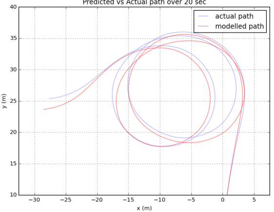
Figure 8: Comparison between actual flight data and its predictions by the simulation model used in POMDSoar for the same input roll commands, over 20s of flight.

With the above method, we have achieved a difference of $<1$ meter between the predicted and actual trajectories. Figure 3 shows the match between the model-predicted and actual bank and aileron deflection angle evolutions for several roll commands, and Figure 8 shows the match between predicted and actual multi-action trajectories typically generated during thermalling.

Importantly, depending on the chosen range of target bank angles that encode the action set, some of these bank angles may sometimes not be achievable by ArduPlane due to its overly conservative built-in stall prevention mechanism. E.g., if the commanded bank angle is $45^{\circ}$, ArduPlane’s stall prevention may override it and only allow the sUAV to bank at $40^{\circ}$, which will cause a discrepancy between the predicted action trajectory and the actual one. In order to avoid this problem, we have introduced the SOAR_NO_STALLPRV parameter to ArduPlane. When set to 1, it turns off stall prevention during thermalling. Using it requires care, since stalls resulting from extreme bank angles can be very difficult to recover from.

VIII-B Experiment Methodology Details and Additional Results

As described in the “Empirical Evaluation” section, our live experiment consisted in flying two identically Radian Pro airframes (one running POMDSoar, another running ArduSoar) simultaneously along the same set of waypoints. In order reduce randomness and potential bias in the outcomes of these flights, we have taken measures to eliminate the following confounding factors from our evaluation:

• Systematic bias due to airframe differences. Despite undergoing the same tuning procedure, one airframe may perform systematically worse than the other due to minor physical differences such as discrepancies in the center of gravity positions, AHRS calibration results, current draw of the electronic equipment (especially the motor), and even dents in the airfoil.

  To minimize their effect, after each flight that counted towards this experiment’s results we switched the assignment of thermalling controllers to airframes. At each test site, POMDSoar and ArduSoar completed an equal number of experimental flights on each sUAV.
  

  Flight ID	1(F)	2(F)	3(F)	4(F)	5(F)	6(F)	7(F)	8(F)	1(V)	2(V)	3(V)	4(V)	5(V)	6(V)
  Airframe with POMDSoar	YT	BT	YT	YT	BT	YT	BT	BT	BT	YT	YT	YT	BT	BT
  BT flight time, minutes (baseline in parentheses)	33(21)	37(30)	30(26)	27(25)	46(30)	27(26)	35(30)	39(26)	41(27)	29(25)	27(25)	27(25)	39(27)	37(25)
  YT flight time, minutes (baseline in parentheses)	32(25)	31(30)	48(29)	40(27)	38(30)	37(29)	35(30)	34(29)	36(27)	45(25)	38(25)	32(25)	39(27)	32(25)

  TABLE I: Raw flight times for the Valley (V) and Field (F) test site for the YellowTail (YT) and BlackTail (BT) sUAV  airframes. Each airframe performed an equal number of flights at each test site running each thermalling controller (4 flights per controller per airframe at the Field, 3 per controller per airframe at the Valley). For each flight, the battery used was recorded. Baseline flight times are the flight times for the combination of that battery and that airframe at that test site without thermalling. These flight times were recorded in a series of separate flights on still days with thermalling turned off.

• Differences in battery properties. Similar to the previous factor, using batteries with the same nominal capacity may nonetheless result in different flight times under the same conditions. This is partly due to slight variability in the battery manufacturing process, and partly due to divergence of battery properties after several recharge cycles.

  In order to eliminate battery performance from the picture, for each combination of airframe $A$, test site (waypoint sequence) $S$, and battery $B$ used in the experiments, on several calm days we measured flight duration with thermalling controllers turned off and recorded the resulting flight times. For each $A$, $S$, and $B$, we call the average of these timings the baseline flight time, denote it $\textit{BaselineFlightTime}_{A,B,S}$, and account for it in our performance measure for each thermalling flight (see Equation 11). In effect, each $\textit{BaselineFlightTime}_{A,B,S}$ is a flight duration estimate for a given $A$, $B$, and $S$ combination when the sUAV is unaided by a thermalling controller.
  

• Wave and other kinds of lift. Although controllers aboard our sUAVs were designed specifically for thermalling, they could chance upon rising air masses of different nature. The combination of hills, trees, and wind in the test site areas could occasionally give rise to orographic and wave lift. Data gathered in such conditions could the distort picture of POMDSoar’s and ArduSoar’s comparative ability to exploit thermals.

  To eliminate this risk, we avoided flying when we suspected wave lift at the test sites. However, given the virtual indistinguishability of orographic lift from low-altitude thermals, which tend to be irregular and turbulent, we included flights that may have involved orographic soaring into the results.
  

• High outcome variance due to chance of finding thermals. Making good use of even a single thermal could substantially increase a sUAV’s flight time. Therefore, discrepancies in the chances of finding thermals — a factor orthogonal to the quality of the thermalling controller itself — could significantly affect flight duration.

  The design of our mission profile (see the “Mission profile” subsection of the “Empirical Evaluation” section in the main paper) is motivated exactly by minimizing flight time variance due to this factor. The relatively small size of our test sites (both $<700$m in diameter), the small range of altitudes, fixed waypoint courses, identical thermal mode triggering mechanisms, and simultaneous flights by both sUAVs mean that both controllers regularly pass through the same locations at similar altitudes within at most minutes of each other. In addition, we don’t use any explicit thermal finding or altitude loss management strategies such McCready’s speed-to-fly or memorizing locations of previous thermal encounters. All of this results in both sUAVs often activating their thermalling controllers repeatedly at the same set of locations during a given flight, sometimes at the same time, indicating that they are likely catching the same thermals.

  In addition, since both controllers are activated using identical conditions, we eliminated flights where one of the sUAVs activated its thermalling controller at least once and the other didn’t at all, because in those cases the difference in flight duration was purely due to the probabilistic nature of thermal detection. There were only a few such flights, a testament to the robustness of the above mission profile, airframe tuning, and thermal mode triggering strategy.
  

Extended Results

Qualitatively, as Figure 7 indicates, POMDSoar outpeformed ArduSoar in 11 out of 14 flights in terms of the measure in Equation 11, and did as well in 2 of the remaining 3. Moreover, the flight time gains POMDSoar provides are appreciably larger compared to ArduSoar’s.

Moreover, Table I appears to indicate that in terms of win/loss outcomes, baseline correction using Equation 11 didn’t make a difference for in any flight. Indeed, every time the sUAV with the bigger absolute flight duration also happened to win according to Equation 11’s relative gain criterion.

These results agree with our hypothesis that in turbulent low-altitude thermals, POMDP-driven exploration and action selection are critical for taking advantage of whatever lift there is.

Quantitatively, however, Table I shows that baseline correction makes a big difference when analyzing relative gains themselves. For instance, based on absolute numbers, one might think that during flight 1(F), the only one that ArduSoar won, ArduSoar won by only a narrow margin. However, as baseline-corrected results in Figure 7 demonstrate, this is not the case — in that particular flight, ArduSoar’s performance was significantly better than POMDSoar’s. Therefore, baseline correction is important to apply in field experiments with many confounding factors, such as when comparing thermalling controllers.

References

- [1] ArduPlane. URL http://ardupilot.org/plane/index.html.
- [2] Mission planner. URL http://ardupilot.org/planner/.
- Akos et al. [2010] Z. Akos, M. Nagy, S. Leven, and T. Vicsek. Thermal soaring flight of birds and unmanned aerial vehicles. Bioinspiration & Biomimetics, 5(4), 2010.
- Allen [2006] M. Allen. Updraft model for development of autonomous soaring uninhabited air vehicles. In Proc. of the 44th AIAA Aerospace Sciences Meeting and Exhibit, 2006. doi: https://doi.org/10.2514/6.2006-1510. URL https://ntrs.nasa.gov/archive/nasa/casi.ntrs.nasa.gov/20060004052.pdf.
- Allen [2005] M. J. Allen. Autonomous soaring for improved endurance of a small uninhabited air vehicle. In Proc. of the 43th AIAA Aerospace Sciences Meeting and Exhibit, 2005.
- Allen and Lin [2007] M.J. Allen and V. Lin. Guidance and control of an autonomous soaring UAV. Technical report, 2007. URL https://ntrs.nasa.gov/archive/nasa/casi.ntrs.nasa.gov/20070022339.pdf.
- Andersson et al. [2012] K. Andersson, I. Kaminer, V. Dobrokhodov, and V. Cichella. Thermal centering control for autonomous soaring; stability analysis and flight test results. Journal of Guidance, Control, and Dynamics, 35(3):963–975, 2012.
- Åström [1965] K. J. Åström. Optimal control of Markov processes with incomplete state information. Journal of Mathematical Analysis and Applications, 10:174–205, 1965.
- Bird et al. [2014] J. J. Bird, J. W. Langelaan, C. Montella, J. Spletzer, and J. Grenestedt. Closing the loop in dynamic soaring. In Proc. of the 54th AIAA Guidance, Navigation and Control Conference and Exhibit, 2014.
- Chakrabarty and Langelaan [2011] A. Chakrabarty and Jack W. Langelaan. Energy-based long-range path planning for soaring-capable uavs. Journal of Guidance, Control and Dynamics, 34(4):1002–1015, 2011.
- Chung et al. [2015] J. J. Chung, N. R. J. Lawrance, and S. Sukkarieh. Learning to soar: Resource-constrained exploration in reinforcement learning. The International Journal of Robotics Research, 34(2):158–172, 2015.
- Daugherty and Langelaan [2014] S. Daugherty and J. W. Langelaan. Improving autonomous soaring via energy state estimation and extremum seeking control. In Proc. of the 52nd AIAA Aerospace Sciences Meeting and Exhibit, 2014.
- Dearden et al. [1999] R. Dearden, N. Friedman, and D. Andre. Model based Bayesian exploration. In Proc. of the Conference on Uncertainty in Artificial Intelligence (UAI), 1999.
- [14] N. T. Depenbusch, J. J. Bird, and Jack W. Langelaan. The autosoar autonomous soaring aircraft part 2: Hardware implementation and flight results. Journal of Field Robotics. doi: 10.1002/rob.21747. URL http://onlinelibrary.wiley.com/doi/10.1002/rob.21747/full.
- Duff [2002] M. Duff. Optimal Learning: Computational Procedures for Bayes-Adaptive Markov Decision Processes. PhD thesis, University of Massachusetts Amherst, Amherst, MA, 2002.
- Edwards [2008] D. Edwards. Implementation details and flight test results of an autonomous soaring controller. In Proc. of the 46th AIAA Guidance, Navigation and Control Conference and Exhibit, 2008. doi: https://doi.org/10.2514/6.2008-7244. URL http://citeseerx.ist.psu.edu/viewdoc/download?doi=10.1.1.559.4025&rep=rep1&type=pdf.
- Edwards and Silberberg [2010] D. J. Edwards and L. M. Silberberg. Autonomous soaring: The montague cross-country challenge. Journal of Aircraft, 47(5):1763–1769, 2010. doi: https://doi.org/10.2514/1.C000287. URL https://arc.aiaa.org/doi/abs/10.2514/1.C000287.
- Filatov and Unbehauen [2000] N. Filatov and H. Unbehauen. Survey of adaptive dual control methods. IEEE Control Theory and Applications, 147:118–128, 2000.
- Fisher et al. [2016] A. Fisher, M. Marino, R. Clothier, S. Watkins, L. Peters, and J. L. Palmer. Emulating avian orographic soaring with a small autonomous glider. Bioinspiration & Biomimetics, 11(1), 2016. URL http://stacks.iop.org/1748-3190/11/i=1/a=016002.
- Garcia et al. [1989] C. E. Garcia, D. M. Prett, and M. Morari. Model predictive control: Theory and practice-a survey. Automatica, 25(3):335–348, 1989.
- Ghavamzadeh et al. [2015] M. Ghavamzadeh, S. Mannor, J. Pineau, and A. Tamar. Bayesian reinforcement learning: A survey. Foundations and Trends in Machine Learning, 8:5-6:359–492, 2015.
- Guez et al. [2013] A. Guez, D. Silver, and P. Dayan. Scalable and efficient bayes-adaptive reinforcement learning based on Monte-Carlo tree search. 48:841–883, 2013. URL http://www0.cs.ucl.ac.uk/staff/d.silver/web/Publications_files/bamcp-jair.pdf.
- Hazard [2010] M. W. Hazard. Unscented Kalman filter for thermal parameter identification. In Proc. of the 48th AIAA Aerospace Sciences Meeting and Exhibit, 2010.
- Julier and Uhlmann [1997] S. J. Julier and J. K. Uhlmann. A new extension of the Kalman filter to nonlinear systems. In Proceeding of AeroSense: The 11th International Symposium on Aerospace/Defense Sensing, Simulation and Controls, volume Multi Sensor Fusion, Tracking and Resource Management II, pages 182–193, 1997.
- Kalman [1960] R.E. Kalman. A new approach to linear filtering and prediction problems. Transactions of the ASME–Journal of Basic Engineering, 82(Series D):35–45, 1960.
- Langelaan [2007] J. W. Langelaan. Long distance/duration trajectory optimization for small UAVs. In Proc. of the 47th AIAA Guidance, Navigation and Control Conference and Exhibit, 2007.
- Langelaan [2008] J. W. Langelaan. Gust energy extraction for mini- and micro- uninhabited aerial vehicles. In Proc. of the 46th AIAA Aerospace Sciences Meeting and Exhibit, 2008.
- Lecarpentier et al. [2017] E. Lecarpentier, S. Rapp, M. Melo, and E. Rachelson. Empirical evaluation of a q-learning algorithm for model-free autonomous soaring. Les Journées Francophones sur la Planification, la Décision et l’Apprentissage pour la conduite de systèmes (JFPDA), 2017.
- Moral [1996] P. Del Moral. Non linear filtering: Interacting particle solution. Markov Processes and Related Fields, 2(4):555–580, 1996.
- N. R. J. Lawrance [2009] S. Sukkarieh N. R. J. Lawrance. A guidance and control strategy for dynamic soaring with a gliding uav. In Proc. of IEEE International Conference on Robotics and Automation (ICRA), pages 3632–3637, 2009. URL http://ieeexplore.ieee.org/abstract/document/5152441/.
- N. R. J. Lawrance [2011] S. Sukkarieh N. R. J. Lawrance. Path planning for autonomous soaring flight in dynamic wind fields. In Proc. of IEEE International Conference on Robotics and Automation (ICRA), pages 2499–2505, 2011. URL http://ieeexplore.ieee.org/abstract/document/5979966/.
- Pineau et al. [2003] J. Pineau, G. Gordon, and S. Thrun. Point-based value iteration: An anytime algorithm for pomdps. In Proc. of International Joint Conference on Artificial Intelligence (IJCAI), pages 1025–1032, 2003.
- Reddy et al. [2016] G. Reddy, A.Celani, T. J. Sejnowski, and M. Vergassola. Learning to soar in turbulent environments. In Proc. of the National Academy of Science (PNAS), 2016.
- Reichmann [1993] H. Reichmann. Cross-Country Soaring. 7th ed. edition, 1993.
- Silver and Veness [2010] D. Silver and J. Veness. Monte-carlo planning in large pomdps. In Proc. of the 23rd International Conference on Neural Information Processing Systems NIPS, pages 2164–2172, 2010. URL http://dl.acm.org/citation.cfm?id=2997046.2997137.
- Slade et al. [2017] P. Slade, P. Culbertson, Z. Sunberg, and M. J. Kochenderfer. Simultaneous active parameter estimation and control using sampling-based bayesian reinforcement learning. In IEEE/RSJ International Conference on Intelligent Robots and Systems (IROS), 2017. URL https://arxiv.org/abs/1707.09055.
- Sutton and Barto [1998] R. S. Sutton and A. G. Barto. Reinforcement Learning: An Introduction. MIT Press, 1998.
- Tabor et al. [2018] S. Tabor, I. Guilliard, and A. Kolobov. ArduSoar: an open-source thermalling controller for resource-constrained autopilots. arXiV, 2018. URL https://arxiv.org/abs/1802.08215.
- Telford [1970] J. W. Telford. Convective plumes in a convective field. Journal of the Atmospheric Sciences, 27(3):347–358, 1970.
- Wharington [1998] J. Wharington. Autonomous Control of Soaring Aircraft by Reinforcement Learning. Doctorate thesis, Royal Melbourne Institute of Technology, Melbourne, Australia, 1998.
- Wharington and Herszberg [1998] J. Wharington and I. Herszberg. Control of a high endurance unmanned air vehicle. In Proc. of the 21st ICAS Congress, 1998.