Vector boson star solutions with a quartic order self-interaction

Abstract

We investigate boson star (BS) solutions in the Einstein-Proca theory with the quartic order self-interaction of the vector field $\lambda(A^{\mu}\bar{A}_{\mu})^{2}/4$ and the mass term $\mu\bar{A}^{\mu}A_{\mu}/2$, where $A_{\mu}$ is the complex vector field and ${\bar{A}}_{\mu}$ is the complex conjugate of $A_{\mu}$, and $\lambda$ and $\mu$ are the coupling constant and the mass of the vector field, respectively. The vector BSs are characterized by the two conserved quantities, the Arnowitt-Deser-Misner (ADM) mass and the Noether charge associated with the global $U(1)$ symmetry. We show that in comparison with the case without the self-interaction $\lambda=0$, the maximal ADM mass and Noether charge increase for $\lambda>0$ and decrease for $\lambda<0$. We also show that there exists the critical central amplitude of the temporal component of the vector field above which there is no vector BS solution, and for $\lambda>0$ it can be expressed by the simple analytic expression. For a sufficiently large positive coupling $\Lambda:=M_{pl}^{2}\lambda/(8\pi\mu^{2})\gg 1$, the maximal ADM mass and Noether charge of the vector BSs are obtained from the critical central amplitude and of ${\cal O}[\sqrt{\lambda}M_{pl}^{3}/\mu^{2}\ln(\lambda M_{pl}^{2}/\mu^{2})]$, which is different from that of the scalar BSs, ${\cal O}(\sqrt{\lambda_{\phi}}M_{pl}^{3}/\mu_{\phi}^{2})$, where $\lambda_{\phi}$ and $\mu_{\phi}$ are the coupling constant and the mass of the complex scalar field.

I Introduction

The recent detection of gravitational waves (GWs) from merging black holes (BHs) and neutron stars (NSs) by the LIGO and Virgo collaborations Abbott et al. (2016a, b, 2017) has opened new opportunities to test gravitational and fundamental physics in the extremely high density and/or high curvature regions. The near-future detection of GWs will be able to test modifications of general relativity (GR) in strong gravity regimes in terms of the existence of the hairy BHs Berti et al. (2015); Herdeiro and Radu (2015) and the universal relations for NSs Doneva and Pappas (2017).

Although the data of LIGO and Virgo are highly consistent with the theoretical GW waveforms predicted from coalescing BHs and NSs in GR so far, they have not excluded the possibility of modified gravity theories and/or the existence of other more exotic compact objects yet, and the future GW measurements would be able to test them more precisely Berti et al. (2018a, b); Cardoso and Pani (2017). One of the candidates of more exotic compact objects is a boson star (BS) which is a gravitationally bound nontopological solitonic object in a bosonic field theory. If the existence of the BSs could be verified through the near-future GW observations, it may also give us a direct evidence of extra degrees of freedom in modified gravity theories. The BSs are characterized by the two conserved quantities, namely, the Arnowitt-Deser-Misner (ADM) mass $M$ and the Noether charge $Q$ associated with the global $U(1)$ symmetry of the field space. $M$ and $Q$ correspond to the gravitational mass and the number of particles inside a BS system, respectively, and a BS is gravitationally bound if it possesses the positive binding energy, $\mu_{\phi}Q-M>0$, where $\mu_{\phi}$ is the mass of the scalar field. The BS solutions have been first constructed in the Einstein-scalar theory with the mass term $\mu_{\phi}^{2}|\phi|^{2}/2$ Kaup (1968); Ruffini and Bonazzola (1969); Friedberg et al. (1987); Jetzer (1992). The radial perturbation analysis about the BS solutions Gleiser (1988); Jetzer (1992); Lee and Pang (1989); Gleiser and Watkins (1989) has revealed that the critical solutions dividing the stable BSs and the unstable ones correspond to those with the maximal ADM mass and Noether charge Gleiser and Watkins (1989); Hawley and Choptuik (2000). GW signatures of the binary BSs would be distinguishable from those of the binary BHs and NSs as the consequence of the different tidal deformabilities Sennett et al. (2017).

The maximal ADM mass depends on the potential of the scalar field Schunck and Mielke (2003). In the Einstein-scalar theory only with the mass term $\mu_{\phi}^{2}|\phi|^{2}/2$, it is of ${\cal O}(M_{pl}^{2}/\mu_{\phi})$, where $M_{pl}=\sqrt{\hbar c/G}=1.221\times 10^{19}{\rm GeV}/c^{2}$ is the Planck mass (in the rest we work in the units of $c=\hbar=1$), which is much smaller than the Chandrasekhar mass for fermions with the mass $\mu_{\phi}$, of ${\cal O}(M_{pl}^{3}/\mu_{\phi}^{2})$, by assuming that $\mu_{\phi}\ll M_{pl}$. In the theory with both the quartic order self-interaction $\lambda_{\phi}|\phi|^{4}/4$ as well as the mass term $\lambda_{\phi}|\phi|^{2}/2$, it becomes of the same order as the Chandrasekhar mass for the ferminons with the mass $\mu_{\phi}$, of ${\cal O}(\sqrt{\lambda_{\phi}}M_{pl}^{3}/\mu_{\phi}^{2})$ Colpi et al. (1986).

The BS solutions exist not only in the Einstein-scalar theory but also in the Einstein-Proca theory Brito et al. (2016); Landea and Garcia (2016); Brihaye et al. (2017). In the Einstein-Proca theory with the mass term $\mu^{2}\bar{A}^{\mu}A_{\mu}/2$, where $A_{\mu}$ is the vector field and $\bar{A}_{\mu}$ is the complex conjugate of $A_{\mu}$, the properties of the vector BSs are quite similar to those of the BSs in the Einstein-scalar theory with the mass term Brito et al. (2016). The critical solution dividing the stable and unstable vector BSs corresponds to the solution with the maximal ADM mass and Noether charge, and the maximal ADM mass of a vector BS is of ${\cal O}(M_{pl}^{2}/\mu)$.

The question which we addreess in this paper is how the maximal ADM mass and Noether charge of the BS solutions in the Einstein-Proca theory with the quartic order self-interaction of the vector field $\lambda(\bar{A}^{\mu}A_{\mu})^{2}/4$ as well as the mass term $\mu^{2}\bar{A}^{\mu}A_{\mu}/2$ are related to the mass and coupling constant of the vector field, $\mu$ and $\lambda$, and whether they are similar to those in the Einstein-scalar theory with the quartic order self-interaction. The solutions of nontopological solitions in the complex vector field theories with the nonlinear self-interaction potential in the flat and curved spacetimes have been presented in Refs. Loginov (2015); Brihaye and Verbin (2017); Brihaye et al. (2017). While the results presented in this paper have some overlap with those presented in Ref. Brihaye et al. (2017), we focus more on the role of the quartic order self-interaction in the self-gravitating vector BS backgrounds, and derive the quantitative dependence of the physical properties of the BSs on $\lambda$.

The paper is constructed as follows: In Sec. II, we introduce the Einstein-Proca theory with the mass and the quartic order self-interaction, and derive a set of equations to find the structure of the vector BSs. In Sec. III, we numerically construct the vector BS solutions and make arguments about their properties. The last Sec. IV is devoted to giving a brief summary and conclusion.

II Vector boson star solutions

II.1 Theory

We consider the Einstein-Proca theory with the quartic order self-interaction as well as the mass term;

$$S =\int d^{4}x\sqrt{-g}\left[\frac{1}{2\kappa^{2}}R-\frac{1}{4}F^{\mu\nu}{\bar{F}}_{\mu\nu}\right.$$

$$\left.-\frac{1}{2}\mu^{2}A^{\mu}{\bar{A}}_{\mu}-\frac{1}{4}\lambda\left(A^{\mu}{\bar{A}}_{\mu}\right)^{2}\right],$$ (1)

where the greek indices $(\mu,\nu,...)$ run the four-dimensional spacetime, $g_{\mu\nu}$ is the metric tensor, $g^{\mu\nu}:=\left(g_{\mu\nu}\right)^{-1}$, $g={\rm det}(g_{\mu\nu})$ is the determinant of $g_{\mu\nu}$, $R$ is the scalar curvature associated with $g_{\mu\nu}$, $A_{\mu}$ is the complex vector field and $\bar{A}_{\mu}$ is the complex conjugate of $A_{\mu}$, $F_{\mu\nu}:=\partial_{\mu}A_{\nu}-\partial_{\nu}A_{\mu}$ is the field strength and $\bar{F}_{\mu\nu}:=\partial_{\mu}\bar{A}_{\nu}-\partial_{\nu}\bar{A}_{\mu}$ is its complex conjugate, $\kappa^{2}:=8\pi G$ with $G$ being Newton’s constant, $\mu$ is the mass of the complex vector field, and the dimensionless coupling constant $\lambda$ measures the strength of the quartic order self-interaction of the vector field. Throughout the paper we set $c=\hbar=1$, and in these units the Planck mass $M_{pl}$ is given by $M_{pl}=1/\sqrt{G}$. Because of the different sign convention, $\lambda$ in this paper corresponds to $(-\lambda)$ in Refs. Brihaye and Verbin (2017); Brihaye et al. (2017).

Varying the action (II.1) with respect to $g_{\mu\nu}$, we obtain the gravitational field equations of motion (EOM)

$$0={\cal E}_{\mu\nu} :=T^{(A)}_{\mu\nu}-\frac{1}{\kappa^{2}}G_{\mu\nu},$$ (2)

where

$$T^{(A)}_{\mu\nu} :=\frac{1}{2}\left(F_{\mu\rho}{\bar{F}}_{\nu}{}^{\rho}+{\bar{F}}_{\mu\rho}F_{\nu}{}^{\rho}\right)-\frac{1}{4}g_{\mu\nu}F^{\rho\sigma}{\bar{F}}_{\rho\sigma}$$

$$+\frac{\mu^{2}}{2}\left[A_{\mu}{\bar{A}}_{\nu}+A_{\nu}{\bar{A}}_{\mu}-g_{\mu\nu}\bar{A}^{\rho}A_{\rho}\right]$$

$$+\frac{\lambda}{2}\left[\left(\bar{A}^{\rho}A_{\rho}\right)\left(A_{\mu}{\bar{A}}_{\nu}+A_{\nu}{\bar{A}}_{\mu}\right)-\frac{1}{2}g_{\mu\nu}\left(\bar{A}^{\rho}A_{\rho}\right)^{2}\right],$$ (3)

represents the energy-momentum tensor of the vector field. Similarly, varying the action (II.1) with respect to $A_{\mu}$ and $\bar{A}_{\mu}$, we obtain the EOM for the vector field

$$0={\cal F}_{\nu} :=\nabla^{\mu}F_{\mu\nu}-\left[\mu^{2}+\lambda\left(\bar{A}^{\rho}A_{\rho}\right)\right]A_{\nu},$$ (4)

and its complex conjugate $\overline{\cal F}_{\nu}=0$, respectively. Acting the derivative $\nabla^{\nu}$ on Eq. (4), we obtain the constraint relation

$$0={\cal G} :=\nabla^{\nu}\left\{\left[\mu^{2}+\lambda\left(\bar{A}^{\rho}A_{\rho}\right)\right]A_{\nu}\right\}.$$ (5)

Similarly, $\nabla^{\nu}\overline{\cal F}_{\nu}=:\bar{\cal G}=0$. Note that in the theory (II.1) there is the global $U(1)$ symmetry, namely the symmetry under the transformation $A_{\mu}\to e^{i\alpha}A_{\mu}$ where $\alpha$ is a constant, and the associated Noether current is given by

$$j^{\mu}=\frac{i}{2}\left({\bar{F}}^{\mu\nu}A_{\nu}-F^{\mu\nu}{\bar{A}}_{\nu}\right),$$ (6)

which satisfies the conservation law, $\nabla_{\mu}j^{\mu}=0$.

II.2 Static and spherically symmetric spacetime

We consider a static and spherically symmetric spacetime

$$g_{\mu\nu}dx^{\mu}dx^{\nu} =-\sigma(r)^{2}\left(1-\frac{2m(r)}{r}\right)d{\hat{t}}^{2}$$

$$+\left(1-\frac{2m(r)}{r}\right)^{-1}dr^{2}+r^{2}d\Omega_{2}^{2},$$ (7)

where $\hat{t}$ and $r$ are the time and radial coordinates, $d\Omega_{2}^{2}$ is the metric of the unit two sphere, and $m(r)$ and $\sigma(r)$ depend only on the radial coordinate $r$. Correspondingly, we consider the ansatz for the vector field Brito et al. (2016)

$$A_{\mu}dx^{\mu} =e^{-i{\hat{\omega}}{\hat{t}}}\left(a_{0}(r)d{\hat{t}}+ia_{1}(r)dr\right),$$ (8)

where $a_{0}(r)$ and $a_{1}(r)$ depend only on $r$. For the vector BS solutions, the frequency ${\hat{\omega}}$ is assumed to be real and positive, such that the vector field neither grows nor decays in time. The ansatz (8) is compatible with the static and spherically symmetric spacetime (II.2), as it does not give rise to the explicit time dependence of the energy-momentum tensor. In order to find $m$, $\sigma$, $a_{0}$, and $a_{1}$ numerically, we rewrite EOMs (2), (4) and (5) into a set of the evolution equations with respect to $r$.

II.3 Evolution equations

From our ansatz (II.2) and (8), the nontrivial components of the gravitational EOMs (2) are given by

$${\cal E}^{\hat{t}}{}_{\hat{t}}=0,\quad{\cal E}^{r}{}_{r}=0,\quad{\cal E}^{i}{}_{i}=0,$$ (9)

where the indices $(i,j,\cdots)$ run the directions of the two sphere. Similarly, the nontrivial components of the vector field EOM (4) are given by

$${\cal F}_{\hat{t}}=0,\quad{\cal F}_{r}=0.$$ (10)

The complex conjugates of Eq. (10) give the same equations as Eq. (10) and need not be considered separately. All these equations are related by

$$\nabla_{\mu}{\cal E}^{\mu}{}_{r} =-\frac{1}{2}g^{{\hat{t}}{\hat{t}}}\left({\cal F}_{\hat{t}}\times\bar{F}_{{\hat{t}}r}+\bar{\cal F}_{\hat{t}}\times F_{{\hat{t}}r}\right)$$

$$+\frac{1}{2}\left({\cal G}{\bar{A}}_{r}+{\bar{\cal G}}A_{r}\right).$$ (11)

First, ${\cal E}^{\hat{t}}{}_{\hat{t}}=0$ and ${\cal E}^{r}{}_{r}=0$ can be arranged to give the evolution equations for $m$ and $\sigma$ in the $r$ direction as

$$m^{\prime} =F_{m}\left[a_{0},a_{0}^{\prime},a_{1},m,\sigma\right],$$ (12a)

$$\sigma^{\prime} =F_{\sigma}\left[a_{0},a_{1},m,\sigma\right],$$ (12b)

where a prime denotes the derivative with respect to $r$, and $F_{m}$ and $F_{\sigma}$ are the nonlinear combinations of the given variables as

$$F_{m} :=\frac{\kappa^{2}}{8(r-2m)^{2}\sigma^{4}}\left[-3r^{4}\lambda a_{0}^{4}+2r^{2}a_{0}^{2}\left(r\mu^{2}+\lambda a_{1}^{2}(r-2m)\right)(r-2m)\sigma^{2}+\lambda a_{1}^{4}(r-2m)^{4}\sigma^{4}\right.$$

$$\left.+2ra_{1}^{2}(r-2m)^{2}\sigma^{2}\left(r{\hat{\omega}}^{2}+\mu^{2}(r-2m)\sigma^{2}\right)-4r^{2}{\hat{\omega}}a_{1}(r-2m)^{2}\sigma^{2}a_{0}^{\prime}+2r^{2}(r-2m)^{2}\sigma^{2}a_{0}^{\prime 2}\right],$$ (13a)

$$F_{\sigma} :=\frac{\kappa^{2}}{2(r-2m)^{3}\sigma^{3}}\left[-r^{2}\lambda a_{0}^{2}+\left(r\mu^{2}+\lambda a_{1}^{2}(r-2m)\right)(r-2m)\sigma^{2}\right)\left(r^{2}a_{0}^{2}+a_{1}^{2}(r-2m)^{2}\sigma^{2}\right].$$ (13b)

Similarly, ${\cal F}_{\hat{t}}=0$ and ${\cal G}=0$ can be arranged to be

$$a_{0}^{\prime\prime} ={\cal H}^{-1}F_{0}\left[a_{0},a_{0}^{\prime},a_{1},m,m^{\prime},\sigma,\sigma^{\prime}\right],$$ (14a)

$$a_{1}^{\prime} ={\cal H}^{-1}F_{1}\left[a_{0},a_{0}^{\prime},a_{1},m,m^{\prime},\sigma,\sigma^{\prime}\right],$$ (14b)

where $F_{0}$ and $F_{1}$ are regular combinations of the given variables which are too involved to be shown explicitly, and

$${\cal H}:=-r^{2}\lambda a_{0}^{2}+\left(r\mu^{2}+3\lambda a_{1}^{2}\left(r-2m\right)\right)\left(r-2m\right)\sigma^{2}.$$ (15)

Substituting Eqs. (12) into the left-hand side of Eqs. (14) and eliminating $m^{\prime}$ and $\sigma^{\prime}$, we obtain

$$a_{0}^{\prime\prime} ={\cal H}^{-1}\tilde{F}_{0}\left[a_{0},a_{0}^{\prime},a_{1},m,\sigma\right],$$ (16a)

$$a_{1}^{\prime} ={\cal H}^{-1}\tilde{F}_{1}\left[a_{0},a_{0}^{\prime},a_{1},m,\sigma\right],$$ (16b)

where ${\tilde{F}}_{0}$ and $\tilde{F}_{1}$ are regular combinations of the given variables which are also too involved to be shown explicitly.

Equations (12) and (16) are integrated from a point sufficiently close to $r=0$ with the boundary conditions given in Sec. II.4. For a given set of parameters, if ${\cal H}$ vanishes at some finite radius, Eqs. (12) and (16) cannot be integrated further beyond this point, and then no vector BS solution exists.

II.4 Boundary conditions

Solving Eqs. (12) and (16) in the vicinity of $r=0$, we find

$$a_{0} =f_{0}-\frac{f_{0}}{6\sigma_{0}^{2}}\left(f_{0}^{2}\lambda-\mu^{2}\sigma_{0}^{2}+{\hat{\omega}}^{2}\right)r^{2}+{\cal O}\left(r^{4}\right),$$ (17a)

$$a_{1} =-\frac{f_{0}{\hat{\omega}}}{3\sigma_{0}^{2}}r+{\cal O}\left(r^{3}\right),$$ (17b)

$$m =\frac{\kappa^{2}f_{0}^{2}}{24\sigma_{0}^{4}}\left(-3f_{0}^{2}\lambda+2\mu^{2}\sigma_{0}^{2}\right)r^{3}+{\cal O}\left(r^{5}\right),$$ (17c)

$$\sigma =\sigma_{0}+\frac{\kappa^{2}f_{0}^{2}}{4\sigma_{0}^{3}}\left(-f_{0}^{2}\lambda+\mu^{2}\sigma_{0}^{2}\right)r^{2}+{\cal O}\left(r^{4}\right).$$ (17d)

Equation (17) evaluated at $r=r_{1}$ which is sufficiently close to $r=0$ gives the boundary conditions to integrate Eqs. (12) and (16) numerically from $r=r_{1}$ to a sufficiently large value of $r$.

For $\lambda=0$, ${\cal H}$ defined in Eq. (15) never crosses $0$ and the vector BS solutions exist for an arbitrary value of the central amplitude of the temporal component of the vector field, $f_{0}>0$. For $\lambda\neq 0$, expanding ${\cal H}$ in the vicinity of $r=0$ with Eq. (17), we obtain

$${\cal H}=\left(-f_{0}^{2}\lambda+\mu^{2}a_{0}^{2}\right)r^{2}+{\cal O}(r^{4}).$$ (18)

For $\lambda>0$, even if ${\cal H}<0$ in the vicinity of $r=0$, as the ${\cal O}(r^{4})$ terms in Eq. (18) become important, ${\cal H}$ starts to increase and cross $0$. Thus, a regular BS solution can be obtained only for

$$0<f_{0}\leq f_{0,{\rm crit}}:=\frac{\mu\sigma_{0}}{\sqrt{\lambda}},$$ (19)

which was numerically confirmed, where $f_{0,{\rm crit}}$ corresponds to the critical central amplitude of the temporal component of the vector field. On the other hand, for $\lambda<0$, even if ${\cal H}>0$ in the vicinity of $r=0$, the higher order corrections to Eq. (18) make ${\cal H}$ decrease and cross $0$. Thus, also for $\lambda<0$, we numerically confirmed the existence of the critical central amplitude of the temporal component of the vector field $f_{0,{\rm crit}}$, although it cannot be expressed analytically.

For ${\hat{\omega}}$ chosen to be the correct lowest eigenvalue of the vector BS for a given set of parameters, $m$ and $\sigma$ exponentially approach constant values, $m_{\infty}>0$ and $\sigma_{\infty}>0$, respectively, while $a_{0}$ and $a_{1}$ exponentially approach $0$ as $e^{-\sqrt{\mu^{2}-{\hat{\omega}}^{2}/\sigma_{\infty}^{2}}r}$. Thus, the metric exponentially approaches the Schwarzschild form

$$ds^{2} \to-\sigma_{\infty}^{2}\left(1-\frac{2m_{\infty}}{r}\right)d{\hat{t}}^{2}$$

$$+\left(1-\frac{2m_{\infty}}{r}\right)^{-1}dr^{2}+r^{2}d\Omega_{2}^{2},$$ (20)

where the proper time measured by the observer at $r=\infty$ is given by $t=\sigma_{\infty}{\hat{t}}$, and correspondingly the proper frequency $\omega$ is given by

$${\omega}:=\frac{{\hat{\omega}}}{\sigma_{\infty}}.$$ (21)

The condition for the exponential fall-off properties $e^{-\sqrt{\mu^{2}-\omega^{2}}r}$ requires $\omega<\mu$. In the limit $f_{0}\to 0$, $\omega\to\mu$, and the Minkowski solution is obtained.

By the rescalings of

$${\hat{\omega}}\to\frac{{\hat{\omega}}}{\mu},\quad r\to r\mu,\quad m\to\mu m,\quad\sigma\to\sigma,$$

$$a_{0}\to\kappa a_{0},\quad a_{1}\to\kappa a_{1},\quad\lambda\to\frac{\lambda}{\mu^{2}\kappa^{2}},$$ (22)

the evolution equations (12) and (16) can be rewritten into the form without $\mu$ and $\kappa$, and in the rescaled equations the strength of the self-interaction is measured by the dimensionless coupling constant

$$\Lambda:=\frac{\lambda}{\mu^{2}\kappa^{2}}=\frac{M_{pl}^{2}}{(8\pi)\mu^{2}}\lambda.$$ (23)

For the numerical analysis, we may set $\mu=\kappa=1$ and as the result $\lambda=\Lambda$, as it is straightforward to give back the dependence of the physical quantities on $\mu$ and $\kappa$, once the vector BS solutions are numerically obtained for $\mu=\kappa=1$. In addition, as $\sigma_{0}$ corresponds to the degree of freedom of the time rescaling without loss of generality, we may also set $\sigma_{0}=1$. Thus, only the remaining physical parameters are $f_{0}$ and $\Lambda$.

In Figs. 1 and 2, $(m,\sigma)$ and $(a_{0},a_{1})$ are shown as the functions of $r$ for $\Lambda=10$ and $f_{0}=1/(10\kappa)$, respectively.

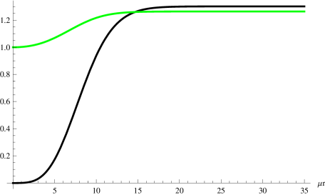
Figure 1: $\mu m$ and $\sigma$ are shown as the functions of $\mu r$ for $\Lambda=10$ and $f_{0}=1/(10\kappa)$. The black and green curves correspond to $\mu m$ and $\sigma$, respectively.

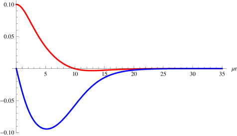
Figure 2: $\kappa a_{0}$ and $\kappa a_{1}$ are shown as the functions of $\mu r$ for $\Lambda=10$ and $f_{0}=1/(10\kappa)$. The red and blue curves correspond to $\kappa a_{0}$ and $\kappa a_{1}$, respectively.

Note that the dimensionless quantities introduced in (II.4) are different from those introduced in Ref. Brihaye et al. (2017) where in the dimensionless equations of motion $a_{0}$ and $a_{1}$ are rescaled to the dimensionless quantities, $(\sqrt{|\lambda|}/\mu)a_{0}$ and $(\sqrt{|\lambda|}/\mu)a_{1}$, respectively. While Ref. Brihaye et al. (2017) focused on the importance of the coupling to gravity measured by the dimensionless parameter $\alpha:=(\kappa^{2}\mu^{2})/\lambda[=1/\Lambda]$ on the nontopological soliton backgrounds in the flat spacetime, we focus more on the role of the quartic order self-interaction of the vector field on the self-gravitating vector BS backgrounds, and derive the quantitative dependence of the physical properties of BSs on the coupling constant $\lambda$. Thus, although there are similarities of our results to those in Ref. Brihaye et al. (2017), we make arguments about the properties of the vector BSs from the different perspectives. In contrast to the case of the scalar BSs, in the case of the vector BSs $a_{0}$ has a single node before approaching $0$.

II.5 ADM mass, Noether charge, and binding energy

We then evaluate the conserved quantities characterizing the vector BSs. The first is the ADM mass

$$M:=\frac{m_{\infty}}{G}=M_{pl}^{2}m_{\infty},$$ (24)

which is associated with the time translational symmetry. The second is the Noether charge associated with the global $U(1)$ symmetry, which is given by integrating $j^{\hat{t}}$ in Eq. (6) over a constant-${\hat{t}}$ hypersurface

$$Q=\int_{\Sigma}d^{3}x\sqrt{-g}j^{\hat{t}}=4\pi\int_{0}^{\infty}dr\frac{r^{2}a_{1}\left({\hat{\omega}}a_{1}-a_{0}^{\prime}\right)}{\sigma}.$$ (25)

A BS is gravitationally bound when $\mu Q-M>0$, and we then define the relative binding energy

$$b:=\frac{B}{M}=\frac{\mu Q}{M}-1.$$ (26)

In order to discriminate various compact objects and classify their physical properties, it is important to define the effective compactness of the vector BS

$${\cal C}:=\frac{GM}{{\cal R}}=\frac{m_{\infty}}{{\cal R}},$$ (27)

where the effective radius of it is given by Schunck and Mielke (2003)

$${\cal R} :=\frac{1}{Q}\int_{\Sigma}d^{3}x\sqrt{-g}\left(rj^{\hat{t}}\right)=\frac{4\pi}{Q}\int_{0}^{\infty}dr\frac{r^{3}a_{1}\left({\hat{\omega}}a_{1}-a_{0}^{\prime}\right)}{\sigma}.$$ (28)

II.6 Comparison with the Einstein-scalar theory

Before proceeding to the physical properties of the vector BSs, we briefly review the case of the Einstein-scalar theory with the quartic order self-interaction

$$S =\int d^{4}x\sqrt{-g}\left[\frac{1}{2\kappa^{2}}R-\frac{1}{2}g^{\mu\nu}\partial_{\mu}\phi\partial_{\nu}\bar{\phi}\right.$$

$$\left.-\frac{1}{2}\mu_{\phi}^{2}|\phi|^{2}-\frac{1}{4}\lambda_{\phi}|\phi|^{4}\right],$$ (29)

where $\mu_{\phi}$ and $\lambda_{\phi}$ are the mass and coupling constant of the complex scalar field, respectively. In the case without the self-interaction, $\lambda_{\phi}=0$, the maximal ADM mass is given as Jetzer (1992); Schunck and Mielke (2003),

$$M_{\rm max}\simeq 0.633\frac{M_{pl}^{2}}{\mu_{\phi}},$$ (30)

which is much smaller than the Chandrasekhar mass for fermions with the same mass. On the other hand, in the case of $\lambda_{\phi}\left(M_{pl}/\mu_{\phi}\right)^{2}\gg 1$, no upper bound on the central amplitude of the scalar field exists, and the maximal ADM mass is given as Colpi et al. (1986),

$$M_{\rm max}\simeq 0.062\sqrt{\lambda_{\phi}}\frac{M_{pl}^{3}}{\mu_{\phi}^{2}}.$$ (31)

Moreover, as shown in Fig. 2 the vector BS solution has a single node in $a_{0}$, while the scalar BS solution has no node in $|\phi|$. In Sec. III we obtain the corresponding relation to Eq. (31) for the vector BSs in the presence of the self-interaction $\lambda(\bar{A}^{\mu}A_{\mu})^{2}/4$.

III Properties of Vector Boson Stars

In this section, we make arguments about the properties of the vector BS solutions in the theory (II.1) obtained numerically.

III.1 ADM mass and Noether charge

In Fig. 3, the ADM mass $M$ and the Noether charge multiplied by $\mu$, $\mu Q$, are shown as the functions of $f_{0}$ for several values of $\Lambda\geq 0$ defined in Eq. (23). We numerically confirmed that there exists the critical central amplitude of the temporal component of the vector field, $f_{0,{\rm crit}}$, and that it agrees with Eq. (19). The behavior for $0<\Lambda\lesssim 1$ is qualitatively similar to that for $\Lambda=0$ except for the existence of $f_{0,{\rm crit}}$; namely $M$ and $Q$ take the local maximal values at some intermediate value of $f_{0}$. For $\Lambda>1$, $M$ and $Q$ monotonically increase for increasing values of $f_{0}$, and their maximal values are obtained from the limit of $f_{0}\to f_{0,\rm crit}$.

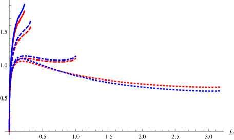
Figure 3: $M$ and $\mu Q$ are shown as the functions of $f_{0}$ for $\Lambda>0$. The red and blue curves correspond to $M$ and $\mu Q$, respectively. The solid, dashed, dot-dashed, and dotted curves correspond to $\Lambda=20,10,1,0.1$, respectively. $(M,\mu Q$) and $f_{0}$ are shown in $M_{pl}^{2}/\mu$ and $M_{pl}/\sqrt{8\pi}[=1/\kappa]$, respectively.

On the other hand, although we do not show the plots of $M$ and $\mu Q$ as the functions of $f_{0}$ for $\Lambda<0$, the values of $M$ and $Q$ become smaller than those for $\Lambda=0$ for the same values of $f_{0}$. For any value of $\Lambda<0$, we numerically confirmed that there is also the critical amplitude of the temporal component of the vector field $f_{0,\rm crit}$, which cannot be expressed analytically and becomes smaller for larger $|\Lambda|$. The maximal values of $M$ and $Q$ correspond to their local maximal values obtained at the intermediate value of $f_{0}<f_{0,{\rm crit}}$. Note that for all the values of $\Lambda$, $M=Q=0$ and the Minkowski solution with the vanishing vector field $A_{\mu}=0$ is obtained for $f_{0}=0$.

In Fig. 4, $M$ is shown as the function of $\omega$ defined in Eq. (21) for $\Lambda>0$. While for $\Lambda=0$ the well-known spiraling behavior is observed as shown in Ref. Brito et al. (2016) and hence $M$ is the multivalued function of $\omega$, $M$ eventually increases and becomes the single-valued function of $\omega$ for $0.1\lesssim\Lambda\lesssim 1$. Furthermore, for $\Lambda\gtrsim 1$, $M$ becomes the monotonically decreasing function of $\omega$. Note that a quantitatively very similar behavior is obtained for $\mu Q$.

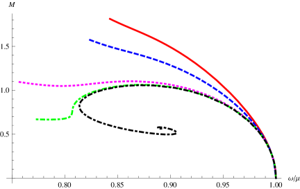
Figure 4: $M$ is shown as the function of $\omega/\mu$ for $\Lambda\geq 0$. The red, blue, magenta, green, and black curves correspond to the cases of $\Lambda=20,10,1,0.1,0$, respectively. $M$ is shown in $M_{pl}^{2}/\mu$.

In Fig. 5, $M$ and $\mu Q$ are compared for $\Lambda=10,1,0.1$, respectively. For all the cases, the solutions with the maximal values of $M$ and $Q$ satisfy $M<\mu Q$, namely, $b>0$ in Eq. (26), and these vector BSs are gravitationally bound. For $\Lambda\lesssim 0.1$, $b<0$ for the smaller values of $\omega$ which are obtained from the values of $f_{0}$ very close to the critical value $f_{0,\rm crit}$, $f_{0}\lesssim f_{0,{\rm crit}}$. For $\Lambda\approx 1$, the values of $M$ and $\mu Q$ obtained from the limit of $f_{0}\to f_{0,{\rm crit}}$ become comparable to the local maximal values of $M$ and $\mu Q$ obtained at the intermediate value of $f_{0}<f_{0,{\rm crit}}$, respectively. For $\Lambda\gtrsim 1$, we obtain $b>0$ for all values of $\omega$.

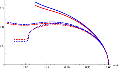
Figure 5: $M$ and $\mu Q$ are compared as the functions of $\omega/\mu$ for $\Lambda>0$. The red and blue curves correspond to $M$ and $\mu Q$, respectively. The solid, dashed, and dotted curves correspond to $\Lambda=10,1,0.1$, respectively. $M$ and $\mu Q$ are shown in $M_{pl}^{2}/\mu$.

In Fig. 6, $M$ is shown as the function of $\omega$ for $\Lambda\leq 0$. As $|\Lambda|$ increases, $M$ decreases for a fixed value of $f_{0}$. Because of the existence of the critical central amplitude of the temporal component of the vector field $f_{0,\rm crit}$, for larger values of $|\Lambda|$ the spiraling behavior is eventually resolved. The maximal value of $M$ is obtained for $f_{0}<f_{0,\rm crit}$. The quantitatively similar behavior is obtained for $\mu Q$.

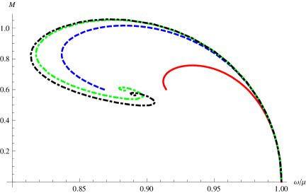
Figure 6: $M$ is shown as the function of $\omega/\mu$ for $\Lambda\leq 0$. The red, blue, green, and black curves correspond to the cases of $\Lambda=-10,-1,-0.1,0$, respectively. $M$ is shown in $M_{pl}^{2}/\mu$.

In Fig. 7, $M$ and $\mu Q$ are compared for $\Lambda<0$. The maximal values of $M$ and $\mu Q$ always satisfy $b>0$.

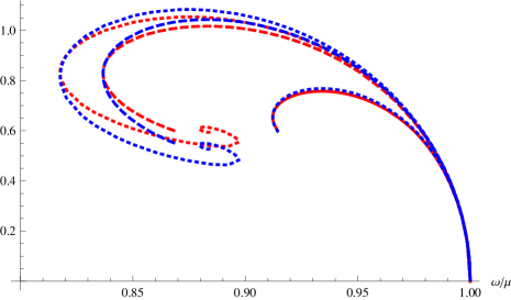
Figure 7: $M$ and $\mu Q$ are compared as the functions of $\omega/\mu$ for $\Lambda<0$. The red and blue curves correspond to $M$ and $\mu Q$, respectively. The solid, dashed, and dotted curves correspond to $\Lambda=-10,-1,-0.1$, respectively. $M$ and $\mu Q$ are shown in $M_{pl}^{2}/\mu$.

We speculate that the disappearance of the spiraling behavior is due to the combination of the two effects which were argued so far. The first is the existence of the critical central amplitude of the temporal component of the vector field $f_{0,{\rm crit}}$, as discussed in Sec. II.4. As $|\Lambda|$ increases, $f_{0,{\rm crit}}$ decreases, and hence the allowed region of the central amplitude, $0<f_{0}\leq f_{0,{\rm crit}}$, shrinks. The second is the overall enhancement of the ADM mass and the Noether charge, due to the stronger self-interaction for $\Lambda>0$, as seen in Figs. 4 and 5.

III.2 Maximal ADM mass and Noether charge

In Fig. 8, the maximal values of $M$ and $\mu Q$, which from now on are denoted by $M_{\rm max}$ and $\mu Q_{\rm max}$, respectively, are shown as the functions of $\Lambda$. They are monotonically increasing for increasing $\Lambda$. As already seen in Sec. III.1, $M_{\rm max}$ and $\mu Q_{\rm max}$ obtained for $\Lambda\lesssim 1$ have a different physical origin from those obtained for $\Lambda\gtrsim 1$, which can be observed as the break around $\Lambda\simeq 1$. From $\Lambda\gg 1$, $M_{\rm max}$ and $\mu Q_{\rm max}$ correspond to the values of $M$ and $Q$ from the limit of $f_{0}\to f_{0,\rm crit}$, respectively. From the data of $M_{\rm max}$ and $\mu Q_{\rm max}$ for $20\leq\Lambda\leq 50$, the fitting formulas

$$M_{\rm max} \approx\frac{M_{pl}^{2}}{\mu}\left[1.383-0.005099\frac{\sqrt{\lambda}M_{pl}}{\mu}\right.$$

$$\left.+\left(-0.03967+0.005675\frac{\sqrt{\lambda}M_{pl}}{\mu}\right)\ln\left(\frac{\lambda M_{pl}^{2}}{\mu^{2}}\right)\right],$$ (32a)

$$\mu Q_{\rm max} \approx\frac{M_{pl}^{2}}{\mu}\left[1.500-0.001989\frac{\sqrt{\lambda}M_{pl}}{\mu}\right.$$

$$\left.+\left(-0.05386+0.005694\frac{\sqrt{\lambda}M_{pl}}{\mu}\right)\ln\left(\frac{\lambda M_{pl}^{2}}{\mu^{2}}\right)\right],$$ (32b)

are obtained, respectively, which can also fit the data of $M_{\rm max}$ and $\mu Q_{\rm max}$ for $50<\Lambda\leq 250$ very well. Thus, for a sufficiently large value of $\Lambda\gg 1$, $M_{\rm max}$ and $\mu Q_{\rm max}$ become of ${\cal O}[\sqrt{\lambda}M_{pl}^{3}/\mu^{2}\ln(\lambda M_{pl}^{2}/\mu^{2})]$, which is different from the case of the BS solutions in the Einstein-scalar theory (31). Note that for $\Lambda=0$ we recover

$$M_{\rm max}\approx 1.058M_{pl}^{2}/\mu,\quad\mu Q_{\rm max}\approx 1.088M_{pl}^{2}/\mu,$$ (33)

obtained in Ref. Brito et al. (2016).

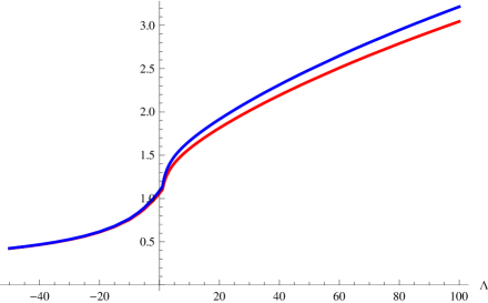
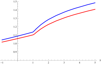
Figure 8: $M_{\rm max}$ and $\mu Q_{\rm max}$ are shown as the functions of $\Lambda$. The red and blue points correspond to $M_{\rm max}$ and $\mu Q_{\rm max}$, respectively. They are shown in $M_{pl}^{2}/\mu$. The lower panel is the enlarged display of the upper one around $\Lambda=1$.

III.3 Binding energy, compactness, and stability

In Fig. 9, the relative binding energy defined in Eq. (26) for the vector BS solutions with $M_{\rm max}$ and $\mu Q_{\rm max}$, $b_{\rm max}:=\mu Q_{\rm max}/M_{\rm max}-1$, is shown as the function of $\Lambda$. The black curve $(\Lambda<1)$ corresponds to the cases in which $M_{\rm max}$ and $\mu Q_{\rm max}$ correspond to their local maximal values obtained at the intermediate value of $f_{0}<f_{0,{\rm crit}}$, while the red curve $(\Lambda>1)$ corresponds to the cases in which $M_{\rm max}$ and $\mu Q_{\rm max}$ obtained at the intermediate value of $f_{0}<f_{0,{\rm crit}}$. Note that for all the values of $\Lambda$, $b_{\rm max}>0$, and hence the vector BS solutions with $M_{\rm max}$ and $\mu Q_{\rm max}$ are always gravitationally bound. For $\Lambda\lesssim 1$, $b_{\rm max}$ is an increasing function of $\Lambda$, while for $\Lambda\gtrsim 1$ it rapidly increases but eventually approaches the constant value $\simeq 0.056$.

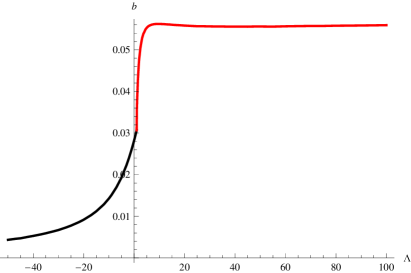
Figure 9: $b_{\rm max}:=\mu Q_{\rm max}/M_{\rm max}-1$ is shown as the function of $\Lambda$. The black curve corresponds to the cases in which $M_{\rm max}$ and $\mu Q_{\rm max}$ correspond to their local maximal values obtained at the intermediate value of $f_{0}<f_{0,{\rm crit}}$, while the red curve corresponds to the case in which $M_{\rm max}$ and $\mu Q_{\rm max}$ are obtained from the limit of $f_{0}\to f_{0,{\rm crit}}$.

In Fig. 10, the compactness ${\cal C}$ defined in Eq. (27) for the vector BS solutions with $M_{\rm max}$ and $\mu Q_{\rm max}$ is shown as the function of $\Lambda$. The black curve corresponds to the cases in which $M_{\rm max}$ and $\mu Q_{\rm max}$ correspond to their local maximal values obtained at the intermediate value of $f_{0}<f_{0,{\rm crit}}$, while the red curve corresponds to the case in which $M_{\rm max}$ and $\mu Q_{\rm max}$ are obtained from the limit of $f_{0}\to f_{0,{\rm crit}}$. The clear discontinuity on the value of ${\cal C}$ exists around $\Lambda=1$. For $\Lambda\gtrsim 1$, ${\cal C}$ is always larger than $0.2$, but cannot exceed $0.32$. Since photon spheres could be formed for a spherically symmetric compact object whose compactness is greater than $1/3=0.333\cdots$, no photon spheres would be formed around the vector BSs. For $\Lambda<1$ including negative values, ${\cal C}$ is less than $0.2$ and gradually decreases as $|\Lambda|$ increases. Note that the compactness (27) was defined with the effective radius ${\cal R}$ defined in (28) outside which the vector field $A_{\mu}$ does not completely vanish and the spacetime geometry is not precisely given by the vacuum Schwarzschild solution.

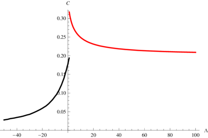
Figure 10: ${\cal C}$ for the solutions with $M_{\rm max}$ and $\mu Q_{\rm max}$ is shown as the function of $\Lambda$. The black curve corresponds to the cases in which $M_{\rm max}$ and $\mu Q_{\rm max}$ correspond to their local maximal values obtained at the intermediate value of $f_{0}<f_{0,{\rm crit}}$, while the red curve corresponds to the case in which $M_{\rm max}$ and $\mu Q_{\rm max}$ are obtained from the limit of $f_{0}\to f_{0,{\rm crit}}$.

In order to see how the effective compactness depends on the definition of the effective radius, ${\cal C}$ defined in Eq. (27) is compared with another definition of the effective compactness, for example,

$$\tilde{\cal C}:=\frac{GM}{\tilde{\cal R}}=\frac{m_{\infty}}{\tilde{\cal R}},$$ (34)

for another definition of the effective radius

$$\tilde{\cal R}:=\left(\int_{0}^{\infty}dr\,r^{3}\rho^{(A)}\right)\Big{/}\left(\int_{0}^{\infty}dr\,r^{2}\rho^{(A)}\right),$$ (35)

where $\rho^{(A)}:=-T^{(A){\hat{t}}}{}_{\hat{t}}$ [see Eq. (II.1)] is the energy density of the vector field Schunck and Mielke (2003). In Fig. 11, the ratio $\tilde{\cal C}/{\cal C}[={\cal R}/\tilde{\cal R}]$ for the solutions with $M_{\rm max}$ and $\mu Q_{\rm max}$ is shown as the function of $\Lambda$. The black curve $(\Lambda<1)$ corresponds to the cases in which $M_{\rm max}$ and $\mu Q_{\rm max}$ correspond to their local maximal values obtained at the intermediate value of $f_{0}<f_{0,{\rm crit}}$, while the red curve $(\Lambda>1)$ corresponds to the cases in which $M_{\rm max}$ and $\mu Q_{\rm max}$ obtained at the intermediate value of $f_{0}<f_{0,{\rm crit}}$. We find that for all values of $\Lambda$, $\tilde{\cal C}/{\cal C}>1$ and hence $\tilde{\cal R}/{\cal R}<1$, but the deviation from unity is at most 9%, namely, $(\tilde{\cal C}/{\cal C})_{\rm max}-1<0.09$. The maximal deviation from unity arises for $\Lambda\simeq 1$, where $\tilde{\cal C}/{\cal C}\simeq 1.087$. As $|\Lambda|$ increases, $\tilde{\cal C}/{\cal C}$ decreases toward unity. Thus, in most cases the difference between ${\cal C}$ and $\tilde{\cal C}$ is not so quantitatively significant. But for the solutions with $\Lambda\simeq 1$, $\tilde{\cal C}$ takes the maximal value $\tilde{\cal C}>0.34$ which exceeds $1/3$, while ${\cal C}<0.32$. Therefore, the ambiguity in the definition of the effective compactness around $\Lambda\simeq 1$ makes it unclear whether photon spheres can be formed around the most compact vector BSs in the presence of the quartic order self-interaction, or not. For the more precise comparison with the other compact objects such as the BHs or NSs more careful analyses are requested, and the possible formation of the photon spheres should be judged by explicitly analyzing null geodesics around the vector BSs, which will be left for a future study.

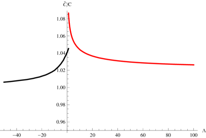
Figure 11: $\tilde{\cal C}/{\cal C}[={\cal R}/\tilde{\cal R}]$ for the solutions with $M_{\rm max}$ and $\mu Q_{\rm max}$ is shown as the function of $\Lambda$. The black curve corresponds to the cases in which $M_{\rm max}$ and $\mu Q_{\rm max}$ correspond to their local maximal values obtained at the intermediate value of $f_{0}<f_{0,{\rm crit}}$, while the red curve corresponds to the case in which $M_{\rm max}$ and $\mu Q_{\rm max}$ are obtained from the limit of $f_{0}\to f_{0,{\rm crit}}$.

As we mentioned in Sec. I, for $\Lambda=0$ the vector BS solution with $M_{\rm max}$ and $\mu Q_{\rm max}$ corresponds to the critical solution which divides the stable and unstable vector BS solutions Brito et al. (2016), as in the case of the scalar BS solutions Gleiser and Watkins (1989); Hawley and Choptuik (2000). As mentioned previously, for all the values of $\Lambda$ the vector BS solutions with $M_{\rm max}$ and $\mu Q_{\rm max}$ satisfy $M_{\rm max}<\mu Q_{\rm max}$, and they are always gravitationally bound. For $\Lambda\lesssim 1$ the solutions with $M_{\rm max}$ and $\mu Q_{\rm max}$ obtained from their local maximal values are also expected to be dynamically stable, and for $\Lambda\gtrsim 1$ those with $M_{\rm max}$ and $\mu Q_{\rm max}$ obtained from the limit of $f_{0}\to f_{0,{\rm crit}}$ would also be dynamically stable. Thus, for all values of $\Lambda$ the vector BS solution with $M_{\rm max}$ and $\mu Q_{\rm max}$ is expected to be stable.

IV Conclusion

In this paper, we have investigated the BS solutions in the Einstein-Proca theory with the quartic order self-interaction as well as the mass (II.1). While the properties of the BS solutions in the Einstein-Proca theory with the mass $\mu^{2}\bar{A}^{\mu}A_{\mu}/2$ have a lot of similarities with those of the BS solutions in the Einstein-scalar theory with the mass $\mu_{\phi}^{2}|\phi|^{2}/2$, we have found that once the quartic order self-interaction $\lambda(\bar{A}^{\mu}A_{\mu})^{2}/4$ is included into the action, the properties of the vector BS solutions become very distinct from those of the scalar BS solutions with the quartic order self-interaction $\lambda_{\phi}|\phi|^{4}/4$.

First, we have formulated the basic equations to find the BS solutions in the Einstein-Proca theory. Assuming the static and spherically symmetric metric ansatz (II.2) and the monochromatic oscillation of the vector field in time (8), the EOM could be rewritten into a set of the evolution equations in the radial direction (12) and (16). Then, the boundary conditions for the metric and vector field variables were derived by solving the evolution equations in the vicinity of the center. For the frequencies chosen to be the eigenvalues of the BS solutions, Eqs. (12) and (16) were able to be numerically integrated, and the metric exponentially approaches the Schwarzschild form (II.4), while the two components of the vector field exponentially approach $0$.

The clear difference between the cases of the scalar and vector fields appearing in the presence of the quartic order self-interaction was that in the case of the Einstein-Proca theory there is the critical amplitude of the temporal component of the vector field at the center, above which no vector BS solution could be obtained. Moreover, it was found that the qualitative behavior of the vector BSs was different across $\Lambda\simeq 1$, where $\Lambda$ is the dimensionless coupling constant defined in Eq. (23). For $\Lambda\lesssim 1$, including the negative values of $\Lambda$, the behavior of the BS solutions was very similar to the case of $\Lambda=0$. In this case, the maximal values of the ADM mass and Noether charge correspond to their local maximal values obtained at the intermediate value of $f_{0}<f_{0,{\rm crit}}$, and the compactness defined in Eq. (27) could not exceed $0.20$. On the other hand, for $\Lambda>1$, they could be obtained from the critical central amplitude of the temporal component of the vector field, and the compactness was always greater than $0.20$ but could not exceed $1/3=0.333\cdots$, below which photon spheres would be absent. However, for the most compact vector BS solutions obtained for $\Lambda\simeq 1$ the ratio of the two different definitions of the effective compactness (27) and (34) was close to $1.09$, and it is still unclear whether the photon spheres could be formed around them or not, which will require further studies. For $\Lambda\gg 1$ the maximal values of the ADM mass and Noether charge could be fitted by the formulas (32), which were of ${\cal O}[\sqrt{\lambda}M_{pl}^{3}/\mu^{2}\ln(\lambda M_{pl}^{2}/\mu^{2})]$, and slightly larger than the Chandrasekhar mass for the fermions with the same mass $\mu$.

There are a lot of remaining issues, e.g., the stability analysis against the radial and nonradial perturbations, the implications for the future gravitational wave observations, and the BS solutions in more general class of the complex vector-tensor theories. They will be left for future work.

References

- Abbott et al. (2016a) B. P Abbott et al. (Virgo, LIGO Scientific), “Observation of Gravitational Waves from a Binary Black Hole Merger,” Phys. Rev. Lett. 116, 061102 (2016a), arXiv:1602.03837 [gr-qc] .
- Abbott et al. (2016b) B. P. Abbott et al. (Virgo, LIGO Scientific), “GW151226: Observation of Gravitational Waves from a 22-Solar-Mass Binary Black Hole Coalescence,” Phys. Rev. Lett. 116, 241103 (2016b), arXiv:1606.04855 [gr-qc] .
- Abbott et al. (2017) B. P. Abbott et al. (Virgo, LIGO Scientific), “GW170817: Observation of Gravitational Waves from a Binary Neutron Star Inspiral,” Phys. Rev. Lett. 119, 161101 (2017), arXiv:1710.05832 [gr-qc] .
- Berti et al. (2015) Emanuele Berti et al., “Testing General Relativity with Present and Future Astrophysical Observations,” Class. Quant. Grav. 32, 243001 (2015), arXiv:1501.07274 [gr-qc] .
- Herdeiro and Radu (2015) Carlos A. R. Herdeiro and Eugen Radu, “Asymptotically flat black holes with scalar hair: a review,” Proceedings, 7th Black Holes Workshop 2014, Int. J. Mod. Phys. D24, 1542014 (2015), arXiv:1504.08209 [gr-qc] .
- Doneva and Pappas (2017) Daniela D. Doneva and George Pappas, “Universal Relations and Alternative Gravity Theories,” (2017), arXiv:1709.08046 [gr-qc] .
- Berti et al. (2018a) Emanuele Berti, Kent Yagi, and Nicolas Yunes, “Extreme Gravity Tests with Gravitational Waves from Compact Binary Coalescences: (I) Inspiral-Merger,” Gen. Rel. Grav. 50, 46 (2018a), arXiv:1801.03208 [gr-qc] .
- Berti et al. (2018b) Emanuele Berti, Kent Yagi, Huan Yang, and Nicolas Yunes, “Extreme Gravity Tests with Gravitational Waves from Compact Binary Coalescences: (II) Ringdown,” Gen. Rel. Grav. 50, 49 (2018b), arXiv:1801.03587 [gr-qc] .
- Cardoso and Pani (2017) Vitor Cardoso and Paolo Pani, “Tests for the existence of black holes through gravitational wave echoes,” Nat. Astron. 1, 586–591 (2017), arXiv:1709.01525 [gr-qc] .
- Kaup (1968) David J. Kaup, “Klein-Gordon Geon,” Phys. Rev. 172, 1331–1342 (1968).
- Ruffini and Bonazzola (1969) Remo Ruffini and Silvano Bonazzola, “Systems of selfgravitating particles in general relativity and the concept of an equation of state,” Phys. Rev. 187, 1767–1783 (1969).
- Friedberg et al. (1987) R. Friedberg, T. D. Lee, and Y. Pang, “MINI - SOLITON STARS,” Phys. Rev. D35, 3640 (1987).
- Jetzer (1992) Philippe Jetzer, “Boson stars,” Phys. Rept. 220, 163–227 (1992).
- Gleiser (1988) Marcelo Gleiser, “Stability of Boson Stars,” Phys. Rev. D38, 2376 (1988).
- Lee and Pang (1989) T. D. Lee and Yang Pang, “Stability of Mini - Boson Stars,” Nucl. Phys. B315, 477 (1989).
- Gleiser and Watkins (1989) Marcelo Gleiser and Richard Watkins, “Gravitational Stability of Scalar Matter,” Nucl. Phys. B319, 733–746 (1989).
- Hawley and Choptuik (2000) Scott H. Hawley and Matthew W. Choptuik, “Boson stars driven to the brink of black hole formation,” Phys. Rev. D62, 104024 (2000), arXiv:gr-qc/0007039 [gr-qc] .
- Sennett et al. (2017) Noah Sennett, Tanja Hinderer, Jan Steinhoff, Alessandra Buonanno, and Serguei Ossokine, “Distinguishing Boson Stars from Black Holes and Neutron Stars from Tidal Interactions in Inspiraling Binary Systems,” Phys. Rev. D96, 024002 (2017), arXiv:1704.08651 [gr-qc] .
- Schunck and Mielke (2003) F.E. Schunck and E.W. Mielke, “General relativistic boson stars,” Class.Quant.Grav. 20, R301–R356 (2003), arXiv:0801.0307 [astro-ph] .
- Colpi et al. (1986) M. Colpi, S. L. Shapiro, and I. Wasserman, “Boson Stars: Gravitational Equilibria of Selfinteracting Scalar Fields,” Phys. Rev. Lett. 57, 2485–2488 (1986).
- Brito et al. (2016) Richard Brito, Vitor Cardoso, Carlos A. R. Herdeiro, and Eugen Radu, “Proca stars: Gravitating Bose-Einstein condensates of massive spin 1 particles,” Phys. Lett. B752, 291–295 (2016), arXiv:1508.05395 [gr-qc] .
- Landea and Garcia (2016) Ignacio Salazar Landea and Federico Garcia, “Charged Proca Stars,” Phys. Rev. D94, 104006 (2016), arXiv:1608.00011 [hep-th] .
- Brihaye et al. (2017) Y. Brihaye, Th. Delplace, and Y. Verbin, “Proca Q Balls and their Coupling to Gravity,” Phys. Rev. D96, 024057 (2017), arXiv:1704.01648 [gr-qc] .
- Loginov (2015) A. Yu. Loginov, “Nontopological solitons in the model of the self-interacting complex vector field,” Phys. Rev. D91, 105028 (2015).
- Brihaye and Verbin (2017) Y. Brihaye and Y. Verbin, “Proca Q Tubes and their Coupling to Gravity,” Phys. Rev. D95, 044027 (2017), arXiv:1611.01803 [gr-qc] .