Single-electron $G^{(2)}$ function at nonzero temperatures

Abstract

The single-particle state is not expected to demonstrate second-order coherence. This proposition, correct in the case of a pure quantum state, is not verified in the case of a mixed state. Here I analyze the consequences of this fact for the second-order correlation function, $G^{(2)}$, of electrons injected on top of the Fermi sea with nonzero temperature. At zero temperature, the function $G^{(2)}$ unambiguously demonstrates whether the injected state is a single- or a multi-particle state: $G^{(2)}$ vanishes in the former case, while it does not vanish in the latter case. However, at nonzero temperatures, when the quantum state of injected electrons is a mixed state, the purely single-particle contribution makes the function $G^{(2)}$ to be non vanishing even in the case of a single-electron injection. The single-particle contribution puts the lower limit to the second-order correlation function of electrons injected into conductors at nonzero temperatures. The existence of a single-particle contribution to $G^{(2)}$ can be verified experimentally by measuring the cross-correlation electrical noise.

I Introduction

Quantum coherent electronics Splettstoesser:2009im ; Haack:2013ch , also known as electron quantum optics Bocquillon:2013fp , and single electron electronics Bauerle:2018ct , is an actively developing platform for quantum information processing Bennett:2000kl , which is aimed at creating, manipulating, and detecting individual electrons as carriers of information.

Recently, quite a lot of single-electron sources on-demand have been experimentally realized.Blumenthal:2007ho ; Feve:2007jx ; Kaestner:2008gv ; Fujiwara:2008gt ; Roche:2013jw ; Dubois:2013ul ; Rossi:2014kp ; Tettamanzi:2014gx ; dHollosy:2015ez ; vanZanten:2016fl ; Gabelli:2016uz ; Rossi:2018wj One of the crucial tests, this source has to pass through, is the verification of a single-particle emission regime.

In quantum optics, the single-photon emission regime is verifies via the measurement of the second-order correlation function, $g^{(2)}$, which characterizes the probability of joint detection of two photons.Walls2008 Such a verification is universal and it does not rely on any specific properties of the source. If the stream generated by a periodically working source consists of non overlapping single photons, then the function $g^{(2)}\left(\tau\right)$ vanishes at zero time delay between the two detections, $\tau=0$. In contrast, if there are multi-photon wave packets in the stream, the two photons can be detected simultaneously and the function $g^{(2)}$ is finite at $\tau=0$.

The measurement of the joint detection probability in the optical frequencies range is possible due to availability of efficient single photon detectors. In the microwave frequencies range, no efficient detectors are available. Nevertheless, the single-particle emission regime for a source of microwave photons Houck:2007dy can be demonstrated via the linear amplification of the magnitude of an electromagnetic field Bozyigit:2010bw .

There are no efficient on-fly detectors available for single electrons so far, and there is no way to measure the magnitude of a fermionic field. This is why for the verification of a single-electron emission regime the various nonuniversal methods were used. The nonuniversality in this context means that the given method can be good for one system, but not for another. In particular, a strong decrease in an electrical noise was used as an indicator of the single-particle emission regime for a dynamical quantum dot Maire:2008hx and for a quantum capacitor Mahe:2010cp ; Albert:2010co ; Parmentier:2012ed , while this method does not work in the case of the source of levitonsDubois:2013ul . Another method for validation of the single-electron injection regime, which is relied on the partition noiseReznikov:1998kn ; Blanter:2000wi of an electron beam splitter, was demonstrated in Refs. Bocquillon:2012if, and Dubois:2013ul, .

Nevertheless, in some systems it is possible to measure directly the second-order correlation function for injected electrons, $G^{(2)}$, which vanishes identically in the case of a single-particle injection. Generally, in the case of electrons injected into an electron waveguide, the second order correlation function contains several contributions: (i) One is due to electrons belonging to the Fermi sea of the waveguide, (ii) one more is due to the injected electrons, that is $G^{(2)}$, (iii) and, finally, the last contribution is due to the joint contribution of the injected electrons and Fermi-sea electrons. Moskalets:2014ea ; Thibierge:2015up As it is pointed out in Ref. Thibierge:2015up, , when electrons are injected into one of the two incoming channels of an electron beam splitter, the cross-correlation noise of currents after the beam splitter is directly related to the function $G^{(2)}$. The Fermi sea electrons do not contribute to the cross-correlation noise either directly or in conjunction with injected electrons. For this to be true, the two conditions must be met. First, the Fermi seas in both incoming channels have the same temperature and the same chemical potential. Second, the incoming and outgoing channels are spatially separated, which can be achieved using chiral or helical edge states Buttiker:2009bg as electron waveguides.

Here I focus on the effect of temperature on the second-order correlation function, $G^{(2)}$, of electrons injected on top of the Fermi sea in conductors. The fact, that at nonzero temperatures the quantum state of injected electrons is a mixed state,Moskalets:2015ub ; Moskalets:2017vk leads to existence of a purely single-particle contribution to the correlation function $G^{(2)}$. This contribution puts the lower limit to the second-order correlation function, and it must be taken into account when the function $G^{(2)}$ is used to distinguish single-electron and multi-electron quantum states.

The paper is organized as follows: In Sec. II I discuss in detail how the correlation function $G^{(2)}$ changes when a pure quantum state becomes a mixed quantum state. In Sec. III the relation between the function $G^{(2)}$ and the current correlation function is given in frequency domain. The temperature dependence of the functions $G^{(2)}$ for single- and two-electron excitations are contrasted in Sec. IV. The conclusion is given Sec. V. Some details of calculations are preseted in the Appendixes A and B.

II Correlation function of electrons injected at nonzero temperatures

A convenient quantity for characterizing the excitations injected by the electron source into the electron waveguide is the excess first-order correlation function, $G^{(1)}$.Grenier:2011js ; Grenier:2011dv ; Moskalets:2013dl To get rid of the contribution of the underlying Fermi sea and keep track of the contribution of injected electrons only, this function is defined as the difference of the two terms, evaluated with the source being switched on and off, respectively, $G^{(1)}\left(1;2\right)=\langle\hat{\Psi}^{{\dagger}}(1)\hat{\Psi}(2)\rangle_{on}-\langle\hat{\Psi}^{{\dagger}}(1)\hat{\Psi}(2)\rangle_{off}$. Here $\hat{\Psi}(j)$ is an electron field operator in second quantization evaluated at time $t_{j}$ and point $x_{j}$, $j=1,2$, after the source. The quantum statistical average, $\langle\dots\rangle$, is performed over the state of electrons in the waveguide before the source. In this work I suppose that the waveguide is one-dimensional, and before the source an electron system is in equilibrium state, which is characterized by the Fermi distribution function with a temperature $\theta$ and a chemical potential $\mu$. Since I am interested in time dependence, rather than spatial dependence, below I keep argument $t_{j}$ only.

Note, the function $G^{(1)}$ for a stream of identically prepared separated electrons in a ballistic conductor was measured in Ref. Jullien:2014ii, using the tomography protocol suggested in Ref. Grenier:2011dv, .

For noninteracting electrons, the first-order correlation function determines the higher-order correlation functions through the corresponding Slater determinants. For example, the second-order correlation function, $G^{(2)}\left(t_{1},t_{2};t_{3},t_{4}\right)$, is determined as follows,

$$G^{(2)}\left(t_{1},t_{2};t_{3},t_{4}\right)=\det\begin{pmatrix}G^{(1)}\left(t_{1};t_{4}\right)&G^{(1)}\left(t_{1};t_{3}\right)\\ G^{(1)}\left(t_{2};t_{4}\right)&G^{(1)}\left(t_{2};t_{3}\right)\end{pmatrix}.$$ (1)

First let us consider a pure quantum state. For a single-particle state ($N=1$) with wave function $\Psi_{1}\left(t\right)$, the first-order correlation function is factorized into the product of two terms that depend on one time each, $G_{N=1}^{(1)}\left(t_{1};t_{2}\right)=\Psi_{1}^{*}\left(t_{1}\right)\Psi_{1}\left(t_{2}\right)$. Apparently, that in this case the second order-correlation function vanishes identically, $G_{N=1}^{(2)}=0$. However, already for a two-particle state ($N=2$), when $G_{N=2}^{(1)}\left(t_{1};t_{2}\right)=\sum_{j=1}^{2}\Psi_{j}^{*}\left(t_{1}\right)\Psi_{j}\left(t_{2}\right)$, the second-order correlation function is not zero. It is represented as follows, $G_{N=2}^{(2)}\left(t_{1},t_{2};t_{3},t_{4}\right)=\Psi_{1,2}^{(2)*}\left(t_{1},t_{2}\right)\Psi_{1,2}^{(2)}\left(t_{4},t_{3}\right)$, where the two-particle wave function,

$$\Psi_{1,2}^{(2)}\left(t_{1},t_{2}\right)=\det\begin{pmatrix}\Psi_{1}\left(t_{1}\right)&\Psi_{2}\left(t_{1}\right)\\ \Psi_{1}\left(t_{2}\right)&\Psi_{2}\left(t_{2}\right)\end{pmatrix},$$ (2)

is the Slater determinant composed of wave functions of both particles, $\Psi_{1}$ and $\Psi_{2}$.

In contrast, in the case of a mixed state, the above relations become essentially modified. The quantum state is now characterize by the density matrix rather than the wave function.

As an example, I consider a mixed state characteristic for electrons injected on top of the Fermi sea at finite temperatures.Moskalets:2017vk The components of such a mixed state are parametrized by a continuous variable, the energy $\epsilon$, with the probability density $p_{\epsilon}=-\partial f\left(\epsilon\right)/\partial\epsilon$, where $f\left(\epsilon\right)=\left(1+e^{\frac{\mu+\epsilon}{k_{B}\theta}}\right)$ is the Fermi distribution function, $k_{B}$ is the Boltzmann constant. So, for the mixed two-particle state, the first-order correlation function reads,Moskalets:2017vk

$$G_{N=2}^{(1)}\left(t_{1};t_{2}\right)=\int d\epsilon p_{\epsilon}\sum_{j=1}^{2}\Psi_{j\epsilon}^{*}\left(t_{1}\right)\Psi_{j\epsilon}\left(t_{2}\right).$$ (3)

Accordingly to Eq. (1), the second-order correlation function becomes,

$$G_{N=2}^{(2)}\left(t_{1},t_{2};t_{3},t_{4}\right)=\int d\epsilon p_{\epsilon}\int d\epsilon^{\prime}p_{\epsilon^{\prime}}\Bigg{\{}$$

$$\Psi_{1\epsilon,2\epsilon^{\prime}}^{(2)*}\left(t_{1},t_{2}\right)\Psi_{1\epsilon,2\epsilon^{\prime}}^{(2)}\left(t_{4},t_{3}\right)$$ (4)

$$+\sum_{j=1}^{2}\Psi_{j\epsilon,j\epsilon^{\prime}}^{*}\left(t_{1},t_{2}\right)\Psi_{j\epsilon,j\epsilon^{\prime}}\left(t_{4},t_{3}\right)\Bigg{\}}.$$

Here the two-particle wave function $\Psi_{1\epsilon,2\epsilon^{\prime}}^{(2)}$ is determined by Eq. (2) with $\Psi_{1}$ being replaced by $\Psi_{1\epsilon}$ and $\Psi_{2}$ being replaced by $\Psi_{2\epsilon^{\prime}}$. In addition, we have a new function $\Psi_{j\epsilon,j\epsilon^{\prime}}$ dependent of two times, which is determined by the Slater determinant composed of different components of the same single-particle mixed state,

$$\Psi_{j\epsilon,j\epsilon^{\prime}}\left(t_{1},t_{2}\right)=\frac{1}{\sqrt{2}}\det\begin{pmatrix}\Psi_{j\epsilon}\left(t_{1}\right)&\Psi_{j\epsilon^{\prime}}\left(t_{1}\right)\\ \Psi_{j\epsilon}\left(t_{2}\right)&\Psi_{j\epsilon^{\prime}}\left(t_{2}\right)\end{pmatrix}.$$ (5)

I name it the two-time wave function. Note, that at coincident times, $t_{1}=t_{2}$, this function is zero, $\Psi_{j\epsilon,j\epsilon^{\prime}}\left(t,t\right)=0$, which is a manifestation of the fermionic nature of an electron.

The contribution to $G^{(2)}$ due to the two-time wave function is present even in the case of a single-particle, but mixed state $\left(N=1\right)$,

$$G_{N=1}^{(2)}\left(t_{1},t_{2};t_{3},t_{4}\right) = \int d\epsilon p_{\epsilon}\int d\epsilon^{\prime}p_{\epsilon^{\prime}}$$

$$\Psi_{1\epsilon,1\epsilon^{\prime}}^{*}\left(t_{1},t_{2}\right)\Psi_{1\epsilon,1\epsilon^{\prime}}\left(t_{4},t_{3}\right).$$

Note, at zero temperature the probability density becomes the delta function of energy, $p_{\epsilon}=\delta\left(\epsilon-\mu\right)$, and the only component with Fermi energy, $\epsilon=\mu$, survives. Since $\Psi_{j\mu,j\mu}\left(t_{1},t_{2}\right)=0$, the second-order correlation function vanishes, $G_{N=1}^{(2)}=0$, at zero temperature, as expected for a (pure) single-particle state.

In contrast, at nonzero temperatures, when $p_{\epsilon}\neq\delta\left(\epsilon-\mu\right)$, a single-particle state demonstrates some degree of second-order coherence, which is quantified by $G^{(2)}_{N=1}\neq 0$. This is somewhat counter-intuitive, since the quantities like $G^{(2)}$ are considered essentially multi-particle in nature.

To resolve this seeming paradox, let us recall the physical meaning of $G^{(2)}$, specifically with pairwise equal arguments, $t_{1}=t_{4}$ and $t_{2}=t_{3}$. For a pure state, it is represented by the square of a two-particle wave function, $G^{(2)}\left(t_{1},t_{2};t_{2},t_{1}\right)=\left|\Psi^{(2)}\left(t_{1},t_{2}\right)\right|^{2}$. The conventional meaning of the wave function square is the detection probability, the probability of a strong, projective measurement. In our case, it is the joint probability of two detections, at time $t_{1}$ and at time $t_{2}$.

In the case of a state with two particles, say, with wave functions $\Psi_{1}(t)$ and $\Psi_{2}(t)$, both detections are possible. Let us suppose that in the first measurement we detect a particle with wave function $\Psi_{1}$ at time $t=t_{1}$. The projective measurement means, that after the detection the wave function is changed, it is reduced to the delta function, $\Psi_{1}(t)\sim\delta\left(t-t_{1}\right)$. Therefore, the original wave function cannot be measured at any other times. However, there is a second particle with wave function $\Psi_{2}(t)$, which can be detected in the second measurement, say, at time $t=t_{2}\neq t_{1}$. Hence, we are able to perform two measurements, and the probability for such a joint measurement is given by $G_{N=2}^{(2)}\left(t_{1},t_{2};t_{2},t_{1}\right)\neq 0$.

The case with a single-particle state is different. As I mentioned above, we can perform a projective measurement on a single particle state only once, say, at $t=t_{1}$, and cannot measure it again $t=t_{2}\neq t_{1}$. This fact is manifested as $G_{N=1}^{(2)}=0$.

However, this logic fails in the case of a mixed state. The reason for this is that a particle in a mixed state can be in several quantum states, components of a mixed state, appearing with some probabilities. In Eqs. (II) and (5) these states are $\Psi_{1\epsilon}$ for various $\epsilon$. When we detect a particle at time $t=t_{1}$, we detect it in some particular component state, say, in the state with $\epsilon=\epsilon_{0}$. As a result this component is reduced to the delta function, $\Psi_{1\epsilon_{0}}(t)\sim\delta\left(t-t_{1}\right)$, and the original wavefunction cannot be measured at any other times. But there are many other components of the mixed state with $\epsilon\neq\epsilon_{0}$. Any of them is available for the next detection, say, at time $t=t_{2}\neq t_{1}$. This is why for a mixed single-particle state the second-order correlation function is not vanishing, $G_{N=1}^{(2)}\neq 0$. Obviously, all higher-order correlation functions are also not vanishing.

The ability of a (mixed) single-particle state to demonstrate the second-order coherence can be verified (or refuted) experimentally. In particular, the function $G^{(2)}$ with pairwise equal arguments is directly accessible through the cross-correlation noise measurement.

III $G^{(2)}$ and the cross-correlation noise

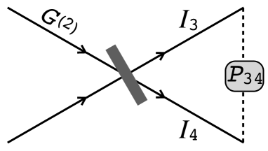
As it was pointed-out in Ref. Thibierge:2015up, , the second-order correlation function with pairwise equal arguments, $G^{(2)}\left(t_{1},t_{2};t_{2},t_{1}\right)$, is directly related to the cross-correlation symmetrized noiseButtiker:1990tn ; Samuelsson:2004uv ; Neder:2007jl ; McClure:2007gl . More precisely, it is related to the currents, $I_{3}\left(t_{1}\right)$ and $I_{4}\left(t_{2}\right)$, and their correlation function, ${P}_{34}\left(t_{1},t_{2}\right)$, which are measured at the outputs of an electronic interferometer Henny:1999tb ; Oliver:1999ws ; Oberholzer:2000wx , analogous to the Hanbury Brown and Twiss (HBT) interferometer HanburyBrown:1956bi known in optics, see Fig. 1. The source of electrons is placed in one of the inputs. The temperature of both input channels $1$ and $2$, with and without an electron source, should be the same, $\theta_{1}=\theta_{2}\equiv\theta$. Since the source injects particles periodically with period ${\cal T}_{0}$, the resulting currents are periodic functions of time, $I_{\alpha}\left(t\right)=I_{\alpha}\left(t+{\cal T}_{0}\right)$, $\alpha=3,4$.

Figure 1: Scheme of an electron HBT interferometer, where the quantum state injected into one of input channels (marked by $G^{(2)}$) is transmitted through and reflected at the wave splitter (shown as a shaded thin rectangle). As a result the outgoing current $I_{3}$ and $I_{4}$ are generated. These currents, together with their cross-correlation function ${P}_{34}$, define the second-order correlation function of injected state, $G^{(2)}$, according to Eq. (9). The arrows show the direction of propagation of electrons.

Since the measurement of a time-resolved noise is challenging, below I focus on a frequency-resolved noiseButtiker:1992vn ; Liu:1994fy ; Lesovik:1994tq ; Pedersen:1998uc ; Salo:2006ie ; Braggio:2016ki ; Dittmann:2018ve , which was measured more than once, see, e.g., Refs. Schoelkopf:1997cc, ; DiCarlo:2006ju, ; ZakkaBajjani:2007gg, and also Ref. Mahe:2010cp, , where, as I already mentioned, a frequency-resolved noise was used for validation of the single-electron injection regime.

Let us introduce the following Fourier transform,

$$G^{(2)}_{\ell}\left(\omega\right)=\int\limits_{0}^{{\cal T}_{0}}dte^{i\Omega\ell t}\int\limits_{-\infty}^{\infty}d\tau e^{i\omega\tau}G^{(2)}\left(t+\tau,t;t,t+\tau\right),$$ (7)

where $\Omega=2\pi/{\cal T}_{0}$ and $\ell$ is an integer. Then, $G^{(2)}_{\ell}\left(\omega\right)$ is expressed in terms of the finite-frequency cross-correlation noise power, ${\cal P}_{34,\ell}\left(\omega\right)$ and outgoing currents $I_{3}$ and $I_{4}$, as follows, (see the Appendix A for the precise definition of ${\cal P}_{34,\ell}\left(\omega\right)$, Eqs. (20) and (21), and for the corresponding derivation within the Floquet scattering matrix approach)

$$v_{\mu}^{2}G^{(2)}_{\ell}\left(\omega\right)=\frac{{\cal P}_{34,\ell}(\omega)}{e^{2}RT/{\cal T}_{0}}$$ (8)

$$+\frac{1}{e^{2}RT}\int\limits_{0}^{{\cal T}_{0}}e^{i\Omega\ell t}dt\int\limits_{-\infty}^{\infty}d\tau e^{i\omega\tau}I_{3}\left(t+\tau\right)I_{4}\left(t\right).$$

Here $T$ and $R=1-T$ are the transmission and reflection probabilities of a wave splitter of an electron HBT interferometer, $v_{\mu}$ is the Fermi velocity of electrons in a waveguide, $e$ is an electron charge.

In the special case, when the excitations produced during different periods do not overlap, the equation (8) can be simplified. We take into account explicitly the fact that the current is periodic, set ${\cal T}_{0}\to\infty$, and introduce a continuous frequency $\omega_{\ell}=\ell\Omega$ instead of the series of discrete frequencies $\ell\Omega$, see Appendix A.4 for details. Then the equation (8) becomes,

$$v_{\mu}^{2}G^{(2)}_{\ell}\left(\omega\right) = \frac{{\cal P}_{34,\ell}(\omega)}{e^{2}RT/{\cal T}_{0}}+\frac{I_{3}\left(\omega\right)I_{4}\left(\omega_{\ell}-\omega\right)}{e^{2}RT/{\cal T}_{0}^{2}}.$$ (9)

This equation resembles Eq. (22) of Ref. Moskalets:2014ea, , where the two-energy distribution function was related to the zero-frequency noise power and DC currents in the circuit with two energy filters, quantum dots each with one working resonant quantum level.

Below, I will use Eq. (9) and address the temperature dependence of $G^{(2)}_{\ell}\left(\omega\right)$ for electrons injected by some particular source, namely the source of levitons Dubois:2013ul , that is capable of generating single- as well as multi-particle excitations Dubois:2013fs ; Gaury:2014jz ; Hofer:2014jb ; Belzig:2016jza ; Suzuki:2017er ; Glattli:2017vp .

IV Example: The source of levitons

The sequence of the Lorentzian voltage pulses,

$$eV(t)=N\sum\limits_{m=-\infty}^{\infty}\frac{2\hbar\Gamma_{\tau}}{\left(t-m{\cal T}_{0}\right)^{2}+\Gamma_{\tau}^{2}}.$$ (10)

applied to a metallic contact, generates the stream of excitations with charge $eN$ each in a ballistic channel attached to the contact. Levitov:1996 ; Ivanov:1997 ; Keeling:2006 Here $\Gamma_{\tau}$ is the half-width of a voltage pulse. These excitations are named $N$-electron levitons or $N$-levitons Ronetti:2017vd .

IV.1 Correlation functions

In the regime, when the period is much larger then the width of a voltage pulse, ${\cal T}_{0}\gg\Gamma_{\tau}$, the excitations created at different periods do not overlap. Then, we can restrict ourselves to a single period only, say, $m=0$, and send ${\cal T}_{0}\to\infty$ in the integrals we need to evaluate. In this case the first-order correlation function of excitations injected by the source of levitons is represented as follows,

$$v_{\mu}G^{(1)}(t_{1};t_{2})=\int\limits d\epsilon p_{\theta}\left(\epsilon\right)\sum\limits_{j=1}^{N}\Psi^{*}_{j,\epsilon}(t_{1})\Psi_{j,\epsilon}(t_{2}).$$ (11)

Here $\Psi_{j,\epsilon}(t)=e^{-it\frac{\mu+\epsilon}{\hbar}}\psi_{j}\left(t\right)$ is the wave function of the $j$th particles comprising an $N$-electron leviton ($j=1,\dots,N$). The corresponding envelope function is the following, Grenier:2013 ; Moskalets:2015vr ; glattli2016method

$$\psi_{j}\left(t\right) = \sqrt{\frac{\Gamma_{\tau}}{\pi}}\frac{1}{t-i\Gamma_{\tau}}\left(\frac{t+i\Gamma_{\tau}}{t-i\Gamma_{\tau}}\right)^{j-1}.$$ (12)

Using the fact that the envelope wave functions, $\psi_{j}$, are independent of energy, we can integrate $\epsilon$ out in Eq. (11) and get,

$$v_{\mu}G^{(1)}(t_{1};t_{2})=\eta\left(\frac{t_{1}-t_{2}}{\tau_{\theta}}\right)\sum\limits_{j=1}^{N}\psi^{*}_{j}(t_{1})\psi_{j}(t_{2}),$$ (13)

where $\eta(x)=x/\sinh(x)$ and the thermal coherence time is $\tau_{\theta}=\hbar/(\pi k_{B}\theta)$.

Substituting the above equation into Eq. (1), one can calculate the second-order correlations function. For $t_{1}=t_{4}$ and $t_{2}=t_{3}$ we have,

$$v_{\mu}^{2}G^{(2)}\left(t_{1},t_{2};t_{2},t_{1}\right)=\sum\limits_{j=1}^{N}\sum\limits_{k=1}^{N}\Bigg{\{}\left|\psi_{j}(t_{1})\right|^{2}\left|\psi_{k}(t_{2})\right|^{2}$$

(14)

$$-\eta^{2}\left(\frac{t_{1}-t_{2}}{\tau_{\theta}}\right)\psi^{*}_{j}(t_{1})\psi_{j}(t_{2})\psi^{*}_{k}(t_{2})\psi_{k}(t_{1})\Bigg{\}}.$$

Now I will analyze the above equation in two cases, $N=1$ and $N=2$.

IV.2 A single-electron leviton, $N=1$

For a single-particle leviton, $N=1$, the function $G^{(2)}$ becomes,

$$v_{\mu}^{2}G_{N=1}^{(2)}\left(t_{1},t_{2};t_{2},t_{1}\right)=\frac{\Gamma_{\tau}^{2}}{\pi^{2}}\frac{1-\eta^{2}\left(\frac{t_{1}-t_{2}}{\tau_{\theta}}\right)}{\left(t_{1}^{2}+\Gamma_{\tau}^{2}\right)\left(t_{2}^{2}+\Gamma_{\tau}^{2}\right)}.$$ (15)

From this equation, we can conclude the following. First, when the time difference is smaller then the thermal coherence time, $\left|t_{1}-t_{2}\right|\ll\tau_{\theta}$, the function $\eta=1$, and the second order correlation function vanishes, $G_{N=1}^{(2)}=0$. This fact is a manifestation of a single-particle nature of a quantum state in question.

Second, at larger time difference, $\left|t_{1}-t_{2}\right|\gg\tau_{\theta}$, the function $\eta=0$, and the second order correlation function is factorized into the product of two terms, each of which depends only on one time, $G_{N=1}^{(2)}\left(t_{1},t_{2};t_{2},t_{1}\right)=\left|\psi_{1}\left(t_{1}\right)\right|^{2}\left|\psi_{1}\left(t_{2}\right)\right|^{2}$. Namely, the two-particle detection probability becomes the product of two statistically independent single-particle detection probabilities. Such a property is expected for a classical rather than a quantum state. Nevertheless, the state of a leviton remains quantum and respects the Pauli exclusion principle, which requires that the function $G^{(2)}$ strictly vanishes at equal times (at any temperature), $G_{N=1}^{(2)}\left(t,t;t,t\right)=0$.

IV.2.1 The frequency representation

Let us perform the Fourier transformation defined in Eq. (7) on the function $G^{(2)}$ of a single leviton, Eq. (15). Using the fact that ${\cal T}_{0}\gg\Gamma_{\tau}$, we get,

$$v_{\mu}^{2}G_{N=1,\ell}^{(2)}\left(\omega\right)=e^{-\left|\omega\right|\Gamma_{\tau}}e^{-\left|\omega-\omega_{\ell}\right|\Gamma_{\tau}}-e^{-\left|\omega_{\ell}\right|\Gamma_{\tau}}$$

$$\times\frac{\Gamma_{\tau}}{\pi}\int\limits_{-\infty}^{\infty}d\tau\frac{\eta^{2}\left(\frac{\tau}{\tau_{\theta}}\right)}{\tau^{2}+4\Gamma_{\tau}^{2}}\bigg{\{}\cos\left(\omega\tau\right)+\cos\left(\left[\omega-\omega_{\ell}\right]\tau\right)$$

$$+\frac{2\Gamma_{\tau}}{\tau}{\rm sgn}(\omega_{\ell})\left[\sin\left(\omega\tau\right)-\sin\left(\left[\omega-\omega_{\ell}\right]\tau\right)\right]\bigg{\}}.$$

(16)

As I already mentioned, this function is experimentally accessible through the finite-frequency noise measurement, see Eq. (9).

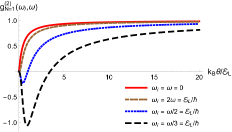
In Fig. 2 I show $G_{N=1,\ell}^{(2)}\left(\omega\right)$, Eq. (16), as a function of temperature for several fixed frequencies. My aim is to show that the function $G^{(2)}_{N=1}$ is capable of demonstrating a crossover from a single-particle behaviour at zero temperature to a multi-particle-like behaviour at nonzero temperatures. Indeed, at zero temperature $G_{N=1,\ell}^{(2)}\left(\omega\right)=0$ for any frequencies, demonstrating that the state in question is a true single-particle state. At nonzero temperatures, the function $G^{(2)}$ becomes different from zero, indicating that the state of a single leviton demonstrates rather multi-particle behaviour. At high temperatures, when the thermal coherence time becomes smaller than the width of a voltage pulse, $\tau_{\theta}\ll\Gamma_{\tau}$, the second-order correlation function achieves its high-temperature asymptotic behaviour, $v_{\mu}^{2}\lim\limits_{\theta\to\infty}G_{N=1,\ell}^{(2)}\left(\omega\right)=e^{-\left|\omega\right|\Gamma_{\tau}}e^{-\left|\omega-\omega_{\ell}\right|\Gamma_{\tau}}$. This product form is characteristic of a completely classical state.

Note, that the growth of $G^{(2)}_{N=1}$ with temperature is manifested in the reduction of single-particle shot noiseDubois:2013fs ; Moskalets:2015ub ; Moskalets:2017dy . The shot noise decrease with increasing temperature was reported in Refs. Bocquillon:2012if, ; Bocquillon:2013fp, ; Glattli:2016wl, ; Glattli:2016tr, .

Figure 2: The second-order correlation function of a single leviton, Eq. (16), normalized to its high-temperature asymptotics, $g_{N=1}^{(2)}\left(\omega_{\ell},\omega\right)=v_{\mu}^{2}G_{N=1,\ell}^{(2)}\left(\omega\right)/\left(e^{-\left|\omega\right|\Gamma_{\tau}}e^{-\left|\omega-\omega_{\ell}\right|\Gamma_{\tau}}\right)$, is given as a function of temperature. The temperature, $k_{B}\theta$, and frequencies, $\hbar\omega$ and $\hbar\omega_{\ell}$, are given in units of the energy of a leviton, ${\cal E}_{L}=\hbar/\left(2\Gamma_{\tau}\right)$.

The temperature dependence of the function $G^{(2)}$ for a multi-electron state is remarkably different. Namely, its zero temperature limit is not universal. On contrary, such a limit depends strongly on frequency. To illustrate this statement, let us consider the case of a $2$-electron leviton.

IV.3 A two-electron leviton, $N=2$

The correlation function of a $2$-electron leviton, $G_{N=2}^{(2)}$, is given in Eq. (11) with $N=2$. The corresponding wave functions are presented in Eq. (12). After performing the Fourier transformation according to Eq. (7), we obtain $G_{N=2,\ell}^{(2)}\left(\omega\right)$, see Eq. (32), which is shown in Fig. 3 as a function of temperature for several fixed frequencies.

Figure 3: The second-order correlation function of a $2$-electron leviton, Eq. (32), normalized to its high-temperature asymptotics, $g_{N=2}^{(2)}\left(\omega_{\ell},\omega\right)=v_{\mu}^{2}G_{N=2,\ell}^{(2)}\left(\omega\right)/\left(4e^{-\left|\omega\right|\Gamma_{\tau}}e^{-\left|\omega-\omega_{\ell}\right|\Gamma_{\tau}}\right)$, is given as a function of temperature. The temperature, $k_{B}\theta$, and frequencies, $\hbar\omega$ and $\hbar\omega_{\ell}$, are given in units of the energy of a leviton, ${\cal E}_{L}=\hbar/\left(2\Gamma_{\tau}\right)$.

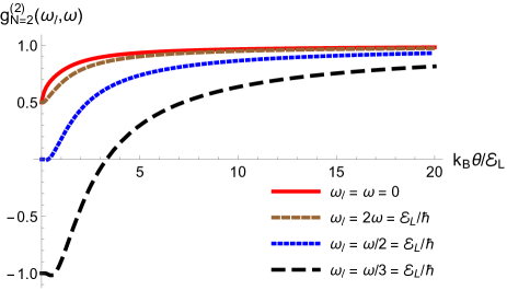
We can see, that at zero temperature, the magnitude of $G_{N=2,\ell}^{(2)}\left(\omega\right)$ is not zero, unlike the case of a plain leviton, $N=1$. Indeed, it strongly depends on the frequencies $\omega_{\ell}$ and $\omega$. Such a nonuniversal frequency-dependent behaviour is characteristic of a multi-particle state, the two-particle state in the present case.

Interestingly, the high-temperature asymptotics of the second-order correlation function of a multi-electron leviton is universal: It is determined by the corresponding asymptotics of the function $G^{(2)}$ of a single-electron leviton,

$$\lim\limits_{\theta\to\infty}G_{N=N_{0}}^{(2)}=N_{0}^{2}\lim\limits_{\theta\to\infty}G_{N=1}^{(2)}.$$ (17)

This is a manifestation of the high-temperature fusion effect (when the multi-electron system behaves like one particle of the total charge) discussed in Ref. Moskalets:2018ch, .

Note, that the low-temperature regime, for which Figs. 2 and 3 show different behaviour, is achievable in present day experiment. So, in Ref. Glattli:2016tr, the voltage pulses with width $2\Gamma_{\tau}=75$ ps were user to generate levitons with energy ${\cal E}_{L}\approx 320$ mK. The experimental data on shot noise were reported for the temperature range from $\theta_{1}=40$ mK to $\theta_{2}=138$ mK. Correspondingly, the ratio $\theta/{\cal E}_{L}$ is changed from $\theta_{1}/{\cal E}_{L}\approx 0.125$ to $\theta_{2}/{\cal E}_{L}\approx 0.43$. From Figs. 2 and 3 we see that for these parameters the function $G^{(2)}$ allows one to uniquely distinguish single-particle and multi-particle states: The second-order correlation function, $G^{(2)}$, is almost constant in the case of a $2$-electron leviton, while it decreases rapidly to zero with decreasing temperature in the case of a single-electron leviton.

V Conclusion

I have discussed the effect of temperature on the second-order correlation function of electrons, $G^{(2)}$, which are injected by an on-demand source on top of the Fermi sea in conductors.

The second-order correlation function is a universal tool that is able to distinguish between single- and multi-particle injection regime of an electron source. The function $G^{(2)}$ is accessible via the cross-correlation electrical noise measurement at the exit of an electron Hanbury Brown and Twiss interferometer.

At zero temperature, the function $G^{(2)}$ is vanishing in the case of a single-electron injection and does not vanish in the case of multi-particle injection. In contrast, at nonzero temperatures, the function $G^{(2)}$ does not vanish even in the case of a single-electron injection. The reason is that at nonzero temperatures, the single-particle quantum state is a mixed state that demonstrates some degree of second-order coherence, which is quantified by $G^{(2)}\neq 0$. Therefore, the existence of this single-particle contribution has to be taken into account, when the second-order correlation function is used for the verification of a single-particle injection into conductors at nonzero temperatures.

Appendix A Electron versus electrical correlation functions

The setup of interest consists of an electron wave splitter, a quantum point contact VanWees:1988vf ; Wharam:1988vi , with two incoming, $\alpha=1,2$, and two outgoing, $\beta=3,4$, one-dimensional wave guides, which are connected to respective metallic leads with the same temperature $\theta$ and chemical potential $\mu$, see Fig. 1. The transmission $T$ and reflection $R=1-T$ probabilities of a wave splitter are energy independent (within the energy range relevant to our problem).

One of the incoming waveguides, say $\alpha=1$, is connected to an electron source that periodically emits particles. The period is denoted as ${\cal T}_{0}$. Within the scattering approach, the periodically working source is characterized by the Floquet scattering matrix $S_{F}$ dependent on two energies, $E$ and $E_{n}=E+n\hbar\Omega$ with $n$ being integer and the frequency $\Omega=2\pi/{\cal T}_{0}$ is dictated by the periodicity. By the virtue of definition, $S_{F}\left(E_{n},E\right)$ is a quantum-mechanical amplitude for the process, when an electron with energy $E$ passing by a source changes its energy to $E_{n}$. Moskalets:2002hu

My aim here is to prove Eq. (8). For this, I use Eq. (1) and write,

$$G^{(2)}\left(t_{1},t_{2};t_{2},t_{1}\right) = -\left|G^{(1)}\left(t_{1};t_{2}\right)\right|^{2}$$

$$+G^{(1)}\left(t_{1};t_{1}\right)G^{(1)}\left(t_{2};t_{2}\right).$$

The first-order correlation function at coincident times defines an electrical current generated by the source, $I(t)=ev_{\mu}G^{(1)}\left(t;t\right)$.Moskalets:2016va The outgoing currents are expressed in terms of the incoming current $I(t)$, as follows, $I_{3}(t)=RI(t)$ and $I_{4}(t)=TI(t)$. The currents are periodic in time, $I(t)=I(t+{\cal T}_{0})$. Therefore, after the Fourier transform defined in Eq. (7), the second line of Eq. (LABEL:a01-2) reproduces the second line of Eq. (8).

To prove that the first term on the right hand side of Eq. (LABEL:a01-2) leads to the first term on the right hand side of Eq. (8), I express both the cross-correlation electrical noise power of the outgoing currents, ${\cal P}_{34}$, and the excess first-order correlation function of electrons injected by the source, $G^{(1)}$, in terms of the Floquet scattering matrix of the source, and then relate them to each other.

A.1 Frequency-dependent electrical noise

The symmetrized cross-correlation function of electrical currents $I_{3}$ and $I_{4}$ flowing out of the wave splitter, see Fig. 1, is defined as follows, Buttiker:1992vr

$${P}_{34}\left(t_{1}.t_{2}\right) = \frac{1}{2}\left\langle\Delta\hat{I}_{3}(t)\Delta\hat{I}_{4}(t+\tau)+\Delta\hat{I}_{4}(t+\tau)\Delta\hat{I}_{3}(t)\right\rangle,$$

where $\Delta\hat{I}_{\alpha}(t)=\hat{I}_{\alpha}(t)-\left\langle\hat{I}_{\alpha}(t)\right\rangle$, $\alpha=3,4$, is an operator of current fluctuations in second quantization. The angle brackets $\left\langle\dots\right\rangle$ denote a quantum-statistical average over the equilibrium state of an incoming single-mode channel not affected by the electron source. Such an equilibrium state is the Fermi sea with a temperature $\theta$ and a chemical potential $\mu$. The other incoming channel of the wave splitter is in the same equilibrium state, with the same temperature $\theta$ and the same chemical potential $\mu$.

For convenience, let us analyze this quantity in frequency representation. In the general non-stationary case, the current correlation function ${P}_{34}$ depends on two frequencies. In the case with periodic driving, the Floquet scattering theory calculations give for our setup,Moskalets:2007dl ; Moskalets2013

$${P}_{34}(\omega,\omega^{\prime}) = 2\pi\sum\limits_{\ell=-\infty}^{\infty}\delta(\omega+\omega^{\prime}-\ell\Omega){\cal P}_{34,\ell}(\omega),$$ (20)

where the noise power ${\cal P}_{34,\ell}(\omega)$ is expressed in terms of the Floquet scattering matrix elements of an electron source, $S_{F}$, as follows,

$${\cal P}_{34,\ell}(\omega)=-RT\frac{e^{2}}{h}\int\limits dE\sum\limits_{n}\sum\limits_{m}\sum\limits_{q}f(E_{q}+\hbar\omega)f(E)$$

(21)

$$\left\{\delta_{n0}\delta_{m+\ell,0}-S_{F}^{*}(E_{n},E)S_{F}(E_{m+\ell},E)\right\}\Big{\{}\delta_{nq}\delta_{mq}$$

$$-S_{F}^{*}(E_{m}+\hbar\omega,E_{q}+\hbar\omega)S_{F}(E_{n}+\hbar\omega,E_{q}+\hbar\omega)\Big{\}}.$$

Here $n,m,q$ are integers, $\delta_{nm}$ is the Kronecker delta, and $f\left(E\right)=\left(1+e^{-\frac{E-\mu}{k_{B}\theta}}\right)^{-1}$ is the Fermi distribution function for electrons in a metallic contact with temperature $\theta$ and chemical potential $\mu$, $k_{B}$ is the Boltzmann constant.

Easy to see that in equilibrium, that is, when the source is turned off and, accordingly, $S_{F}\left(E_{n},E_{m}\right)=\delta_{nm}$, the noise power is zero, ${\cal P}_{34,\ell}(\omega)=0$. So, in our setup, where the contacts $\beta=3$ and $\beta=4$ have no a direct connection between themselves, only the partition noise of injected particles, but not the quantum noise Gardiner2000 , contributes to the measured noise.

For convenience of the subsequent comparison with the electron correlation function, I represent the noise power as the sum of four terms, ${\cal P}_{34,\ell}(\omega)=-RT\frac{e^{2}}{h}\sum_{r=1}^{4}B_{r}$, with

$$B_{1}=\int\limits dE\sum\limits_{n}\sum\limits_{m}\sum\limits_{q}f(E_{q}+\hbar\omega)f(E)\quad\quad$$ (22a)

$$S_{F}^{*}(E_{n},E)S_{F}(E_{m+\ell},E)S_{F}^{*}(E_{m}+\hbar\omega,E_{q}+\hbar\omega)$$

$$S_{F}(E_{n}+\hbar\omega,E_{q}+\hbar\omega),$$

$$\quad\ B_{2}=-\int\limits dE\sum\limits_{q}f(E_{q}+\hbar\omega)f(E)\quad\quad$$ (22b)

$$S_{F}^{*}(E_{q},E)S_{F}(E_{q+\ell},E),$$

$$B_{3}=-\int\limits dE\sum\limits_{q}f(E_{q}+\hbar\omega)f(E)\quad\quad$$ (22c)

$$S_{F}^{*}(E_{-\ell}+\hbar\omega,E_{q}+\hbar\omega)S_{F}(E+\hbar\omega,E_{q}+\hbar\omega),$$

$$B_{4} = \delta_{\ell 0}\int\limits dEf(E+\hbar\omega)f(E).\quad\quad$$ (22d)

Now let us turn to the quantum description of the excitations injected by the source.

A.2 Electron correlation function

As I discussed in Sec. II, the first-order correlation function for these excitations, $G^{(1)}$, is defined as the difference of the electron correlation functions with the source switched on and off, $G^{(1)}\left(t;t^{\prime}\right)=\left\langle\hat{\Psi}^{{\dagger}}\left(t\right)\hat{\Psi}\left(t^{\prime}\right)\right\rangle_{on}-\left\langle\hat{\Psi}^{{\dagger}}\left(t\right)\hat{\Psi}\left(t^{\prime}\right)\right\rangle_{off}$. Here $\hat{\Psi}\left(t\right)$ is a single-particle electron field operator in second quantization at time $t$ just downstream the source. The angle brackets, $\left\langle\dots\right\rangle$, denote the quantum-statistical average over the state of the Fermi sea of electrons approaching the source from the metallic contact $\alpha=1$ being in equilibrium.

I adopt the wide band approximation and suppose that in the waveguides the electron spectrum can be linearized. The Floquet scattering theory expresses $G^{(1)}$ in terms of $S_{F}$ as follows, Moskalets:2015ub

$$G^{(1)}(t;t^{\prime})=\frac{1}{hv_{\mu}}\int dEf\left(E\right)e^{\frac{i}{\hbar}E\left(t-t^{\prime}\right)}\quad\quad$$ (23)

$$\left\{\sum_{n,m=-\infty}^{\infty}e^{i\Omega\left(nt-mt^{\prime}\right)}S_{F}^{*}\left(E_{n},E\right)S_{F}\left(E_{m},E\right)-1\right\}.$$

Note, that the possibility to linearize an electron spectrum is important to perform linear optic-like manipulations with electrons. For instance, if we need to calculate $G^{(1)}$ at another place, say, at a distance $x$ from the source downstream, we simply replace $t\to t-v_{\mu}x$ with $v_{\mu}$ being the Fermi velocity.

The wide band approximation is also crucial to get simple relations between electrical and quantum-mechanical quantities.

A.3 The connection between the two

Now let us demonstrate that the electrical noise power and the electron correlation function squared are related by the following Fourier transformation,

$$\frac{{\cal P}_{34,\ell}(\omega)}{{\cal P}_{0}}=-\int\limits_{0}^{{\cal T}_{0}}e^{i\Omega\ell t}dt\int\limits_{-\infty}^{\infty}d\tau e^{i\omega\tau}\left|v_{\mu}G^{(1)}(t+\tau;t)\right|^{2}.$$

(24)

Here ${\cal P}_{0}=e^{2}RT/{\cal T}_{0}$ is the circuit constant. This constant is the shot noise caused by the scattering of single electrons being in the pure state on a wave splitter at a rate of one particle per period ${\cal T}_{0}$. Blanter:2000wi

The relation analogous to Eq. (24) but for the zero-frequency noise power was presented in Refs. Moskalets:2015ub, ; Moskalets:2017dy, .

To prove Eq. (24), first, let us represent the square of the correlation function, Eq. (23), as the sum of four terms,

$$\left|v_{\mu}G^{(1)}(t;t^{\prime})\right|^{2}=\frac{1}{h^{2}}\sum\limits_{s=1}^{4}A_{s}(t;t^{\prime}),$$ (25a)

$$A_{1}(t;t^{\prime})=\int dEf\left(E\right)e^{\frac{i}{\hbar}E\left(t-t^{\prime}\right)}\int dE^{\prime}f\left(E^{\prime}\right)$$

(25b)

$$e^{\frac{-i}{\hbar}E^{\prime}\left(t-t^{\prime}\right)}\sum_{n,m}e^{i\Omega\left(nt-mt^{\prime}\right)}S_{F}^{*}\left(E_{n},E\right)S_{F}\left(E_{m},E\right)$$

$$\sum_{j,k}e^{-i\Omega\left(jt-kt^{\prime}\right)}S_{F}\left(E_{j}^{\prime},E^{\prime}\right)S_{F}^{*}\left(E_{k}^{\prime},E^{\prime}\right),$$

$$A_{2}(t;t^{\prime})=-\int dEf\left(E\right)e^{\frac{i}{\hbar}E\left(t-t^{\prime}\right)}\int dE^{\prime}f\left(E^{\prime}\right)$$

(25c)

$$e^{\frac{-i}{\hbar}E^{\prime}\left(t-t^{\prime}\right)}\sum_{n,m}e^{i\Omega\left(nt-mt^{\prime}\right)}S_{F}^{*}\left(E_{n},E\right)S_{F}\left(E_{m},E\right),$$

$$A_{3}(t;t^{\prime})=-\int dEf\left(E\right)e^{\frac{i}{\hbar}E\left(t-t^{\prime}\right)}\int dE^{\prime}f\left(E^{\prime}\right)$$

(25d)

$$e^{\frac{-i}{\hbar}E^{\prime}\left(t-t^{\prime}\right)}\sum_{j,k}e^{-i\Omega\left(jt-kt^{\prime}\right)}S_{F}\left(E_{j}^{\prime},E^{\prime}\right)S_{F}^{*}\left(E_{k}^{\prime},E^{\prime}\right),$$

$$A_{4}(t;t^{\prime})=\int dEf\left(E\right)e^{\frac{i}{\hbar}E\left(t-t^{\prime}\right)}\int dE^{\prime}f\left(E^{\prime}\right)e^{\frac{-i}{\hbar}E^{\prime}\left(t-t^{\prime}\right)}.$$

(25e)

As the next step, let us perform the following Fourier transformation,

$$A_{s,\ell}\left(\omega\right)=\frac{1}{h}\int_{0}^{{\cal T}_{0}}\frac{dt}{{\cal T}_{0}}e^{i\Omega\ell t}\int\limits_{-\infty}^{\infty}d\tau e^{i\omega\tau}A_{s}\left(t+\tau,t\right),$$ (26a)

and show that $A_{s,\ell}\left(\omega\right)$ is nothing but $B_{s}$, Eqs. (22).

Let us start with $A_{4}$,

$$A_{4,\ell}\left(\omega\right) = \frac{1}{h}\int_{0}^{{\cal T}_{0}}\frac{dt}{{\cal T}_{0}}e^{i\Omega\ell t}\int\limits_{-\infty}^{\infty}d\tau e^{i\omega\tau}$$

$$\int dEf\left(E\right)e^{\frac{i}{\hbar}E\tau}\int dE^{\prime}f\left(E^{\prime}\right)e^{\frac{-i}{\hbar}E^{\prime}\tau}$$

$$= \delta_{\ell 0}\int dEf\left(E\right)\left(E+\hbar\omega\right).$$

This equation is exactly $B_{4}$, Eq. (22d).

The Fourier transform of $A_{3}$, Eq. (25d), gives us,

$$A_{3,\ell}\left(\omega\right)=-\frac{1}{h}\int_{0}^{{\cal T}_{0}}\frac{dt}{{\cal T}_{0}}e^{i\Omega\ell t}\int\limits_{-\infty}^{\infty}d\tau e^{i\omega\tau}\quad\$$ (26c)

$$\int dEf\left(E\right)e^{\frac{i}{\hbar}E\tau}\int dE^{\prime}f\left(E^{\prime}\right)e^{\frac{-i}{\hbar}E^{\prime}\tau}$$

$$\sum_{j,k}e^{-i\Omega j\tau}e^{-i\Omega t\left(j-k\right)}S_{F}\left(E_{j}^{\prime},E^{\prime}\right)S_{F}^{*}\left(E_{k}^{\prime},E^{\prime}\right)$$

$$=-\int dE\sum_{j}f\left(E\right)f\left(E_{-j}+\hbar\omega\right)$$

$$S_{F}^{*}\left(E_{-\ell}+\hbar\omega,E_{-j}+\hbar\omega\right)S_{F}\left(E+\hbar\omega,E_{-j}+\hbar\omega\right).$$

After replacing $-j$ by $q$ we recognize the above equation as $B_{3}$, Eq. (22c).

The next term is $A_{2}$, Eq. (25c),

$$A_{2,\ell}\left(\omega\right)=-\frac{1}{h}\int_{0}^{{\cal T}_{0}}\frac{dt}{{\cal T}_{0}}e^{i\Omega\ell t}\int\limits_{-\infty}^{\infty}d\tau e^{i\omega\tau}\quad\$$ (26d)

$$\int dEf\left(E\right)e^{\frac{i}{\hbar}E\tau}\int dE^{\prime}f\left(E^{\prime}\right)e^{\frac{-i}{\hbar}E^{\prime}\tau}$$

$$\sum_{n,m}e^{i\Omega n\tau}e^{i\Omega t\left(n-m\right)}S_{F}^{*}\left(E_{n},E\right)S_{F}\left(E_{m},E\right)$$

$$=-\int dE\sum_{n}f\left(E\right)f\left(E_{n}+\hbar\omega\right)$$

$$S_{F}^{*}\left(E_{n},E\right)S_{F}\left(E_{n+\ell},E\right).$$

This is the same as $B_{2}$, Eq. (22b).

And finally, let us calculate the Fourier transform of $A_{1}$, Eq. (25b),

$$A_{1,\ell}\left(\omega\right)=\frac{1}{h}\int\limits_{0}^{{\cal T}_{0}}\frac{dt}{{\cal T}_{0}}e^{i\Omega\ell t}\int\limits_{-\infty}^{\infty}d\tau e^{i\omega\tau}\int dEf\left(E\right)e^{\frac{i}{\hbar}E\tau}\ \ \ \$$ (26e)

$$\int dE^{\prime}f\left(E^{\prime}\right)e^{\frac{-i}{\hbar}E^{\prime}\tau}\sum_{n,m,j,k}e^{i\Omega(n-j)\tau}e^{i\Omega t\left(n+k-m-j\right)}$$

$$S_{F}^{*}\left(E_{n},E\right)S_{F}\left(E_{m},E\right)S_{F}\left(E_{j}^{\prime},E^{\prime}\right)S_{F}^{*}\left(E_{k}^{\prime},E^{\prime}\right)$$

$$=\int dE\sum_{n,m,j}f\left(E\right)f\left(E_{n-j}+\hbar\omega\right)$$

$$S_{F}^{*}\left(E_{n},E\right)S_{F}\left(E_{m},E\right)S_{F}\left(E_{n}+\hbar\omega,E_{n-j}+\hbar\omega\right)$$

$$S_{F}^{*}\left(E_{m-\ell}+\hbar\omega,E_{n-j}+\hbar\omega\right).$$

We denote $q=n-j$ instead of $j$, and get,

$$A_{1,\ell}\left(\omega\right)=\int dE\sum_{q}f\left(E\right)f\left(E_{q}+\hbar\omega\right)\ \ \ \$$ (26f)

$$\sum_{n,m}S_{F}^{*}\left(E_{n},E\right)S_{F}\left(E_{m},E\right)$$

$$S_{F}^{*}\left(E_{m-\ell}+\hbar\omega,E_{q}+\hbar\omega\right)S_{F}\left(E_{n}+\hbar\omega,E_{q}+\hbar\omega\right).$$

After the shift $m-\ell\to m$, we find that this is nothing but $B_{1}$, Eq. (22a). Therefore, Eq. (24) indeed holds.

The proof of Eq. (8) is completed.

A.4 The Fourier transformation for the product of first-order correlation functions

Here I show how the second term on the right hand side of Eq. (9) is calculated from the corresponding term in Eq. (8) in the limit of ${\cal T}_{0}\to\infty$.

The current generated by a periodically driven source is periodic in time, $I_{\alpha}(t)=I_{\alpha}(t+{\cal T}_{0})$, $\alpha=3,4$. Therefore, we can expand it into the Fourier series,

$$I_{\alpha}(t) = \sum\limits_{n=-\infty}^{\infty}e^{-in\Omega t}I_{\alpha,n},$$

(27)

$$I_{\alpha,n} = \int_{0}^{{\cal T}_{0}}\frac{dt}{{\cal T}_{0}}e^{in\Omega t}.$$

In the limit of ${\cal T}_{0}\to\infty$, we introduce a continuous frequency $\omega_{n}=n\Omega$, replace $\sum_{n=-\infty}^{\infty}\to\int d\omega_{n}/\Omega$, and introduce the continuous Fourier transformation,

$$I_{\alpha}\left(\omega_{n}\right) = \int_{-\infty}^{\infty}dte^{i\omega_{n}t}I_{\alpha}\left(t\right),$$

$$I_{\alpha}\left(t\right) = \int_{-\infty}^{\infty}\frac{d\omega_{n}}{\Omega}e^{-i\omega_{n}t}I_{\alpha}\left(\omega_{n}\right).$$

Then we use the second line of above equation in Eq. (8) and get the corresponding term in Eq. (9).

Appendix B The Fourier transform of the function $G^{(2)}$ for a $2$-electron leviton

The first-order correlation function of a $2$-electron leviton, $G_{N=2}^{(1)}$, is given in Eqs. (11) and (12) for $N=2$. The corresponding second-order correlation function reads,

$$G_{N=2}^{(2)}\left(t+\tau,t;t,t+\tau\right)=-\left|G_{N=2}^{(1)}\left(t+\tau;t\right)\right|^{2}$$

(29)

$$+G_{N=2}^{(1)}\left(t;t\right)G_{N=2}^{(1)}\left(t+\tau;t+\tau\right).$$

Now let us apply the Fourier transformation defined in Eq. (24).

B.1 The first term

The Fourier transform of the first term on the right hand side of Eq. (29) determines the finite-frequency noise power,

$$\frac{{\cal P}_{34,\ell}(\omega)}{{\cal P}_{0}}=-\int\limits_{0}^{{\cal T}_{0}}dte^{i\Omega\ell t}\int\limits_{-\infty}^{\infty}d\tau e^{i\omega\tau}\left|v_{\mu}G_{N=2}^{(1)}\left(t+\tau;t\right)\right|^{2}$$

$$=-\frac{\Gamma_{\tau}^{2}}{\pi^{2}}\int\limits_{0}^{{\cal T}_{0}}dte^{i\Omega\ell t}\int\limits_{-\infty}^{\infty}d\tau e^{i\omega\tau}\eta^{2}\left(\frac{\tau}{\tau_{\theta}}\right)$$

(30a)

$$\Bigg{\{}2\frac{1}{\left(t+\tau\right)^{2}+\Gamma_{\tau}^{2}}\frac{1}{t^{2}+\Gamma_{\tau}^{2}}+\frac{1}{\left(t+\tau-i\Gamma_{\tau}\right)^{2}}\frac{1}{\left(t+i\Gamma_{\tau}\right)^{2}}$$

$$+\frac{1}{\left(t+\tau+i\Gamma_{\tau}\right)^{2}}\frac{1}{\left(t-i\Gamma_{\tau}\right)^{2}}\Bigg{\}}.$$

In the case when the levitons created at different periods do not overlap, ${\cal T}_{0}\gg\Gamma_{\tau}$, we can safely extend the limits of integration over $t$ to infinity and introduce a continuous frequency $\omega_{\ell}=\ell\Omega$ instead of the set of discrete frequencies $\ell\Omega$. Then, to integrate over $t$, we use the following auxiliary integrals,

$$2\frac{\Gamma_{\tau}^{2}}{\pi^{2}}\int\limits_{-\infty}^{\infty}dt\frac{e^{i\omega_{\ell}t}}{\left(t+\tau\right)^{2}+\Gamma_{\tau}^{2}}\frac{1}{t^{2}+\Gamma_{\tau}^{2}}=2\frac{\Gamma_{\tau}}{\pi}\frac{e^{-\left|\omega_{\ell}\right|\Gamma_{\tau}}}{\tau^{2}+4\Gamma_{\tau}^{2}}$$

(30b)

$$\times\left\{\begin{array}[]{cc}1+e^{-i\omega_{\ell}\tau}-i\frac{2\Gamma_{\tau}}{\tau}\left(1-e^{-i\omega_{\ell}\tau}\right),&\ell>0,\\ &\\ 1+e^{-i\omega_{\ell}\tau}+i\frac{2\Gamma_{\tau}}{\tau}\left(1-e^{-i\omega_{\ell}\tau}\right),&\ell<0,\end{array}\right.$$ (30f)

and

$$\frac{\Gamma_{\tau}^{2}}{\pi^{2}}\int\limits_{-\infty}^{\infty}dt\frac{e^{i\omega_{\ell}t}}{\left(t+\tau-i\Gamma_{\tau}\right)^{2}}\frac{1}{\left(t+i\Gamma_{\tau}\right)^{2}}=\frac{\Gamma_{\tau}^{2}}{\pi^{2}}\frac{e^{-\left|\omega_{\ell}\right|\Gamma_{\tau}}}{\left(\tau^{2}+4\Gamma_{\tau}^{2}\right)^{2}}$$

(30g)

$$\left\{\begin{array}[]{cc}e^{-i\omega_{\ell}\tau}\bigg{[}-2\pi\omega_{\ell}\left(\tau^{2}-4\Gamma_{\tau}^{2}+4i\Gamma_{\tau}\tau\right)\\ +\frac{4\pi\left(8\Gamma_{\tau}^{3}-6\Gamma_{\tau}\tau^{2}\right)+4\pi i\left(\tau^{3}-12\Gamma_{\tau}^{2}\tau\right)}{\tau^{2}+4\Gamma_{\tau}^{2}}\bigg{]},&\ell>0,\\ &\\ 2\pi\omega_{\ell}\left(\tau^{2}-4\Gamma_{\tau}^{2}+4i\Gamma_{\tau}\tau\right)\\ \\ +\frac{4\pi\left(8\Gamma_{\tau}^{3}-6\Gamma_{\tau}\tau^{2}\right)+4\pi i\left(\tau^{3}-12\Gamma_{\tau}^{2}\tau\right)}{\tau^{2}+4\Gamma_{\tau}^{2}},&\ell<0.\end{array}\right.$$ (30n)

The noise power becomes,

$$\frac{{\cal P}_{34,\ell}(\omega)}{{\cal P}_{0}}=-e^{-\left|\omega_{\ell}\right|\Gamma_{\tau}}\frac{2\Gamma_{\tau}}{\pi}\int\limits_{-\infty}^{\infty}d\tau\frac{\eta^{2}\left(\frac{\tau}{\tau_{\theta}}\right)}{\tau^{2}+4\Gamma_{\tau}^{2}}\Bigg{\{}\quad\quad\quad$$ (30o)

$$e^{i\omega\tau}+e^{i\tau\left(\omega-\omega_{\ell}\right)}-i\frac{2\Gamma_{\tau}}{\tau}{\rm sgn}(\omega_{\ell})\left[e^{i\omega\tau}-e^{i\tau\left(\omega-\omega_{\ell}\right)}\right]$$

$$+\frac{e^{i\tau\left(\omega-\omega_{\ell}\right)}A+e^{i\omega\tau}A^{*}}{\tau^{2}+4\Gamma_{\tau}^{2}}\Bigg{\}},$$

$$A=\Gamma_{\tau}\left|\omega_{\ell}\right|\left(4\Gamma_{\tau}^{2}-\tau^{2}\right)-i4\Gamma_{\tau}^{2}\omega_{\ell}\tau$$

$$+2\Gamma_{\tau}\frac{\left(8\Gamma_{\tau}^{3}-6\Gamma_{\tau}\tau^{2}\right)+i\,{\rm sgn}(\omega_{\ell})\left(\tau^{3}-12\Gamma_{\tau}^{2}\tau\right)}{\tau^{2}+4\Gamma_{\tau}^{2}}.$$

This equation satisfies the general symmetry properties, ${\cal P}_{\ell}\left(\omega\right)={\cal P}_{-\ell}^{*}\left(-\omega\right)$ and ${\cal P}_{\ell}\left(\omega\right)={\cal P}_{\ell}\left(\ell\Omega-\omega\right)$. Moskalets:2009dk To prove the latter one we need to change $\tau\to-\tau$. Moreover, easy to see, that Eq. (30o) is real,

$$\frac{{\cal P}_{34,\ell}(\omega)}{{\cal P}_{0}} = -e^{-\left|\omega_{\ell}\right|\Gamma_{\tau}}\frac{4\Gamma_{\tau}}{\pi}\int\limits_{0}^{\infty}d\tau\frac{\eta^{2}\left(\frac{\tau}{\tau_{\theta}}\right)}{\tau^{2}+4\Gamma_{\tau}^{2}}$$

$$\times\Bigg{\{}B\left[\cos\left(\omega\tau\right)+\cos\left(\left[\omega-\omega_{\ell}\right]\tau\right)\right]$$

$$+C\left[\sin\left(\omega\tau\right)-\sin\left(\left[\omega-\omega_{\ell}\right]\tau\right)\right]\Bigg{\}},$$

$$B = 1+\Gamma_{\tau}\left|\omega_{\ell}\right|\frac{4\Gamma_{\tau}^{2}-\tau^{2}}{\tau^{2}+4\Gamma_{\tau}^{2}}+4\Gamma_{\tau}^{2}\frac{4\Gamma_{\tau}^{2}-3\tau^{2}}{\left(\tau^{2}+4\Gamma_{\tau}^{2}\right)^{2}},$$

$$C = \frac{2\Gamma_{\tau}}{\tau}{\rm sgn}(\omega_{\ell})-4\Gamma_{\tau}^{2}\frac{\omega_{\ell}\tau}{\tau^{2}+4\Gamma_{\tau}^{2}}$$

$$+2\Gamma_{\tau}{\rm sgn}(\omega_{\ell})\frac{\tau^{3}-12\Gamma_{\tau}^{2}\tau}{\left(\tau^{2}+4\Gamma_{\tau}^{2}\right)^{2}}.$$

Note, the above equation is the total cross-correlation noise power, not the excess noise power, which is more convenient in the case of the auto-correlation noise measurement, see, e.g., Ref. Parmentier:2012ed, .

The noise power ${\cal P}_{34,\ell}$, Eq. (LABEL:b02e), vanishes at large frequencies, $\omega,\omega_{\ell}\gg\Gamma_{\tau}^{-1}$. This fact tells us that quantum noiseGardiner2000 , which grows with frequency, is not manifested here.

B.2 The second term

I denote the Fourier transform of the second line of Eq. (29) as $G^{(2),cl}$. Since this part survives at high temperatures, which is expected for the classical contribution, I introduce the superscript “$cl$”. This part is expressed in terms of the Fourier transform of a current, carried by the levitons, $I(t)=ev_{\mu}G_{N=2}^{(1)}\left(t;t\right)$, as follows,

$$G^{(2),cl}_{\ell}\left(\omega\right) = \frac{1}{e^{2}v_{\mu}^{2}}\int\limits_{0}^{{\cal T}_{0}}e^{i\Omega\ell t}dt\int\limits_{-\infty}^{\infty}d\tau e^{i\omega\tau}I(t)I(t+\tau).$$

Then I use the periodicity condition and write, $I(t)=\sum_{n=-\infty}^{\infty}e^{-in\Omega t}I_{n}$. The above equation becomes,

$$G^{(2),cl}_{\ell}\left(\omega\right) = \frac{2\pi{\cal T}_{0}}{e^{2}v_{\mu}^{2}}\sum\limits_{n=-\infty}^{\infty}\delta\left(\omega-n\Omega\right)I_{n}I_{\ell-n}.$$

In the long period limit, when the levitons emitted at different periods do not overlap, I introduce a continuous frequency $\omega_{n}=n\Omega$ and replace the sum by the integral,

$$\sum\limits_{n=-\infty}^{\infty}\to\int\limits_{-\infty}^{\infty}\frac{d\omega_{n}}{\Omega}.$$ (31c)

Correspondingly, the coefficients of a discrete Fourier transformation are replaces by the coefficients of a continuous Fourier transformation, $I_{n}\to I\left(\omega_{n}\right)/{\cal T}_{0}$. Then the equation (LABEL:b03b) becomes,

$$v_{\mu}^{2}G^{(2),cl}_{\ell}\left(\omega\right) = \frac{{\cal T}_{0}^{2}}{e^{2}}I\left(\omega\right)I\left(\omega_{\ell}-\omega\right),$$ (31d)

with $I\left(\omega\right)=ev_{\mu}G_{N=2}^{(1)}\left(\omega\right)$ and $G_{N=2}^{(1)}\left(\omega\right)=2e^{-\left|\omega\right|\Gamma_{\tau}}$.

According to Eq. (9), the sum of Eqs. (LABEL:b02e) and (31d) defines the Fourier transform of the second-order correlation function,

$$v_{\mu}^{2}G_{N=2,\ell}^{(2)}\left(\omega\right)=\frac{{\cal P}_{34,\ell}(\omega)}{{\cal P}_{0}}+v_{\mu}^{2}G^{(2),cl}_{\ell}\left(\omega\right).$$ (32)

The above function is what is plotted in Fig. 3.

References

• (1) J. Splettstoesser, M. Moskalets, and M. Büttiker, Two-Particle Nonlocal Aharonov-Bohm Effect from Two Single-Particle Emitters, Physical Review Letters 103, 076804 (2009).
• (2) G. Haack, M. Moskalets, and M. Büttiker, Glauber coherence of single-electron sources, Physical Review B 87, 201302 (2013).
• (3) E. Bocquillon, V. Freulon, F. D. Parmentier, J.-M. Berroir, B. Plaçais, C. Wahl, J. Rech, T. Jonckheere, T. Martin, Ch. Grenier, D. Ferraro, P. Degiovanni, and G. Fève, Electron quantum optics in ballistic chiral conductors, Ann. Phys. 526, 1–30 (2014).
• (4) C. Bäuerle, D. C. Glattli, T. Meunier, F. Portier, P. Roche, P. Roulleau, S. Takada, and X. Waintal, Coherent control of single electrons: a review of current progress, Reports on progress in physics 81, 056503 (2018).
• (5) C. H. Bennett and D. P. DiVincenzo, Quantum information and computation, Nature 404, 247–255 (2000).
• (6) M. D. Blumenthal, B. Kaestner, L. Li, S. P. Giblin, T. J. B. M. Janssen, M. Pepper, D. Anderson, G. A. C. Jones, and D. A. Ritchie, Gigahertz quantized charge pumping, Nature Physics 3, 343 (2007).
• (7) G. Fève, A. Mahé, J.-M. Berroir, T. Kontos, B. Plaçais, D. C. Glattli, A. Cavanna, B. Etienne, and Y. Jin, An on-demand coherent single-electron source, Science 316, 1169 (2007).
• (8) B. Kaestner, V. Kashcheyevs, S. Amakawa, M. D. Blumenthal, L. Li, T. J. B. M. Janssen, G. Hein, K. Pierz, T. Weimann, U. Siegner, and H. W. Schumacher, Single-parameter nonadiabatic quantized charge pumping, Physical Review B 77, 153301 (2008).
• (9) A. Fujiwara, K. Nishiguchi, and Y. Ono, Nanoampere charge pump by single-electron ratchet using silicon nanowire metal-oxide-semiconductor field-effect transistor, Applied Physics Letters 92, 042102 (2008).
• (10) B. Roche, R. P. Riwar, B. Voisin, E. Dupont-Ferrier, R. Wacquez, M. Vinet, M. Sanquer, J. Splettstoesser, and X. Jehl, A two-atom electron pump, Nature Communications 4, 1581 (2013).
• (11) J. Dubois, T. Jullien, F. Portier, P. Roche, A. Cavanna, Y. Jin, W. Wegscheider, P. Roulleau, and D. C. Glattli, Minimal-excitation states for electron quantum optics using levitons, Nature 502, 659 (2013).
• (12) A. Rossi, T. Tanttu, K. Y. Tan, I. Iisakka, R. Zhao, K. W. Chan, G. C. Tettamanzi, S. Rogge, A. S. Dzurak, and M. Möttönen, An accurate single-electron pump based on a highly tunable silicon quantum dot, Nano Letters 14, 3405–3411 (2014).
• (13) G. C. Tettamanzi, R. Wacquez, S. Rogge, Charge pumping through a single donor atom, New Journal of Physics 16, 063036 (2014).
• (14) S. d’Hollosy, M. Jung, A. Baumgartner, V. A. Guzenko, M. H. Madsen, J. Nygård, and C. Schönenberger, Gigahertz Quantized Charge Pumping in Bottom-Gate-Defined InAs Nanowire Quantum Dots, Nano Letters 15, 4585–4590 (2015).
• (15) D. M. T. van Zanten, D. M. Basko, I. M. Khaymovich, J. P. Pekola, H. Courtois, and C. B. Winkelmann, Single Quantum Level Electron Turnstile, Physical Review Letters 116, 166801 (2016).
• (16) J. Gabelli, K. Thibault, G. Gasse, C. Lupien, and B. Reulet, Characterization and control of charge transfer in a tunnel junction, Phys. Stat. Sol. (b) 254, 1600619 (2017).
• (17) A. Rossi, J. Klochan, J. Timoshenko, F. E. Hudson, M. Möttönen, S. Rogge, A. S. Dzurak, V. Kashcheyevs, and G. C. Tettamanzi, Gigahertz Single-Electron Pumping Mediated by Parasitic States, arXiv:1803.00791.
• (18) D. F. Walls and G. J. Milburn, Quantum Optics (Springer, 2008).
• (19) A. A. Houck, D. I. Schuster, J. M. Gambetta, J. A. Schreier, B. R. Johnson, J. M. Chow, J. Majer, L. Frunzio, M. H. Devoret, S. M. Girvin, and R. J. Schoelkopf, Generating single microwave photons in a circuit, Nature 449, 328–331 (2007).
• (20) D. Bozyigit, C. Lang, L. Steffen, J. M. Fink, C. Eichler, M. Baur, R. Bianchetti, P. Leek, S. Filipp, M. P. da Silva, A. Blais, and A. Wallraff, Antibunching of microwave-frequency photons observed in correlation measurements using linear detectors, Nature Physics 7, 154–158 (2010).
• (21) N. Maire, F. Hohls, B. Kaestner, K. Pierz, H. W. Schumacher, and R. J. Haug, Noise measurement of a quantized charge pump, Applied Physics Letters 92, 082112 (2008).
• (22) A. Mahé, F.D. Parmentier, E. Bocquillon, J.-M. Berroir, D. C. Glattli, T. Kontos, B. Plaçais, G. Fève, A. Cavanna, and Y. Jin, Current correlations of an on-demand single-electron emitter, Physical Review B 82, 201309(R) (2010).
• (23) M. Albert, C. Flindt, and M. Büttiker, Accuracy of the quantum capacitor as a single-electron source, Physical Review B 82, 041407(R) (2010).
• (24) F. D. Parmentier, E. Bocquillon, J.-M. Berroir, D. C. Glat tli, B. Plaçais, and G. Fève, M. Albert, C. Flindt, and M. Büttiker, Current noise spectrum of a single-particle emitter: Theory and experiment, Physical Review B 85, 165438 (2012).
• (25) M. Reznikov, R. de-Picciotto, and M. Heiblum, D. C. Glattli, A. Kumar, and L. Saminadayar, Quantum shot noise, Superlattices and Microstructures 23, 901–915 (1998).
• (26) Y. M. Blanter, and M. Büttiker, Shot noise in mesoscopic conductors, Physics Reports 336, 1–166 (2000).
• (27) E. Bocquillon, F. D. Parmentier, C. Grenier, J.-M. Berroir, P. Degiovanni, D. C. Glattli, B. Plaçais, A. Cavanna, Y. Jin, and G. Fève, Electron Quantum Optics: Partitioning Electrons One by One, Physical Review Letters 108, 196803 (2012).
• (28) M. Moskalets, Two-electron state from the Floquet scattering matrix perspective, Physical Review B 89, 045402 (2014).
• (29) E. Thibierge, D. Ferraro, B. Roussel, C. Cabart, A. Marguerite, G. Fève, and P. Degiovanni, Two-electron coherence and its measurement in electron quantum optics, Physical Review B 93, 081302 (2016).
• (30) M. Büttiker, Edge-State Physics Without Magnetic Fields, Science 325, 278–279 (2009).
• (31) M. Moskalets and G. Haack, Single-electron coherence: finite temperature versus pure dephasing, Physica E: Low-dimensional Systems and Nanostructures 75, 358–369 (2016).
• (32) M. Moskalets, Single-particle emission at finite temperatures, Low Temp. Phys. 43, 865–76 (2017).
• (33) C. Grenier, R. Hervé, G. Fève, and P. Degiovanni, Electron quantum optics in quantum hall edge channels. Mod. Phys. Lett. B 25, 1053 (2011).
• (34) C. Grenier, R. Hervé, E. Bocquillon, F. D. Parmentier, B. Plaçais, J.-M. Berroir, G. Fève, and P. Degiovanni, Single-electron quantum tomography in quantum Hall edge channels, New Journal of Physics 13, 093007 (2011).
• (35) M. Moskalets, G. Haack, and M. Büttiker, Single-electron source: Adiabatic versus nonadiabatic emission, Physical Review B 87, 125429 (2013).
• (36) T. Jullien, P. Roulleau, B. Roche, A. Cavanna, Y. Jin, and D. C. Glattli, Quantum tomography of an electron, Nature 514, 603–607 (2014).
• (37) M. Büttiker, Scattering theory of thermal and excess noise in open conductors, Physical Review Letters 65, 2901–2904 (1990).
• (38) P. Samuelsson, E. V. Sukhorukov, and M. Büttiker, Two-particle Aharonov-Bohm effect and entanglement in the electronic Hanbury Brown–Twiss setup. Physical Review Letters 92, 026805 (2004).
• (39) I. Neder, N. Ofek, Y. Chung, M. Heiblum, D. Mahalu, and V. Umansky, Interference between two indistinguishable electrons from independent sources, Nature 448, 333–337 (2007).
• (40) D. T. McClure, L. DiCarlo, Y. Zhang, H. A. Engel, and C. M. Marcus, M. P. Hanson and A. C. Gossard, Tunable Noise Cross Correlations in a Double Quantum Dot, Physical Review Letters 98, 056801 (2007).
• (41) M. Henny, S. Oberholzer, C. Strunk, T. Heinzel, K. Ensslin, M. Holland, C. Schönenberger, The Fermionic Hanbury Brown and Twiss Experiment, Science 284, 296 (1999).
• (42) W. D. Oliver, J. Kim, R. C. Liu, and Y. Yamamoto, Hanbury Brown and Twiss-type experiment with electrons, Science 284, 299 (1999).
• (43) S. Oberholzer, M. Henny, C. Strunk, C. Schönenberger, T. Heinzel, K. Ensslin, and M. Holland, The Hanbury Brown and Twiss experiment with fermions, Physica E: Low-dimensional Systems and Nanostructures 6, 314 (2000).
• (44) R. Hanbury Brown and R. Q. Twiss, A Test of a New Type of Stellar Interferometer on Sirius, Nature 178, 1046 (1956).
• (45) M. Büttiker, Role of scattering amplitudes in frequency-dependent current fluctuations in small conductors,. Physical Review B 45, 3807 (1992).
• (46) R. C. Liu and Y. Yamamoto, Nyquist noise in the transition from mesoscopic to macroscopic transport. Physical Review B 50, 17411–17414 (1994).
• (47) G. B. Lesovik and L. S. Levitov, Noise in an ac biased junction: Nonstationary Aharonov-Bohm effect, Physical Review Letters 72, 538–541 (1994).
• (48) M. H. Pedersen and M. Büttiker, Scattering theory of photon-assisted electron transport, Physical Review B 58, 12993 (1998).
• (49) J. Salo, F. Hekking, and J. P. Pekola, Frequency-dependent current correlation functions from scattering theory, Physical Review B 74, 125427 (2006).
• (50) A. Braggio, M. Carrega, D. Ferraro, and M. Sassetti, Finite frequency noise spectroscopy for fractional Hall states at ν= 5/2, J. Stat. Mech. 5, 054010 (2016).
• (51) N. Dittmann and J. Splettstoesser, Finite-frequency noise of interacting single-electron emitters: spectroscopy with higher noise harmonics, arXiv:1805.03130.
• (52) R. Schoelkopf, P. Burke, A. Kozhevnikov, D. Prober, and M. Rooks, Frequency Dependence of Shot Noise in a Diffusive Mesoscopic Conductor, Physical Review Letters 78, 3370–3373 (1997).
• (53) L. DiCarlo, Y. Zhang, D. T. McClure, C. Marcus, L. N. Pfeiffer, and K. W. West, A system for measuring auto- and cross-correlation of current noise at low temperatures, Rev. Sci. Instrum. 77, 073906 (2006).
• (54) E. Zakka-Bajjani, J. Ségala, F. Portier, P. Roche, and D. C. Glattli, A. Cavanna, and Y. Jin, Experimental Test of the High-Frequency Quantum Shot Noise Theory in a Quantum Point Contact, Physical Review Letters 99, 236803 (2007).
• (55) J. Dubois, T. Jullien, C. Grenier, P. Degiovanni, P. Roulleau, and D. C. Glattli, Integer and fractional charge Lorentzian voltage pulses analyzed in the framework of photon-assisted shot noise, Physical Review B 88, 085301 (2013).
• (56) B. Gaury and X. Waintal, Dynamical control of interference using voltage pulses in the quantum regime,. Nature Communications 5, 3844 (2014).
• (57) P. P. Hofer and C. Flindt, Mach-Zehnder interferometry with periodic voltage pulses, Physical Review B 90, 235416 (2014).
• (58) W. Belzig and M. Vanević, Elementary Andreev processes in a driven superconductor–normal metal contact, 75, 22–27 (2016).
• (59) T. J. Suzuki, Coherent transport of levitons through the Kondo resonance, Physical Review B 95, 241302 (2017).
• (60) D. C. Glattli, and P. Roulleau, Pseudorandom binary injection of levitons for electron quantum optics, Physical Review B 97, 125407 (2018).
• (61) L. S. Levitov, H. Lee, and G. B. Lesovik, Electron counting statistics and coherent states of electric current, J. Math. Phys. 37, 4845 (1996).
• (62) D. A. Ivanov, H. W. Lee, and L. S. Levitov, Coherent states of alternating current, Physical Review B 56, 6839 (1997).
• (63) J. Keeling, I. Klich, and L. S. Levitov, Minimal Excitation States of Electrons in One-Dimensional Wires, Physical Review Letters 97, 116403 (2006).
• (64) F. Ronetti, L. Vannucci, D. Ferraro, T. Jonckheere, J. Rech, T. Martin, and M. Sassetti, Crystallization of Levitons in the fractional quantum Hall regime, arXiv:1712.07094.
• (65) C. Grenier, J. Dubois, T. Jullien, P. Roulleau, D. C. Glattli, and P. Degiovanni, Fractionalization of minimal excitations in integer quantum Hall edge channels, Physical Review B 88, 085302 (2013).
• (66) M. Moskalets, First-order correlation function of a stream of single-electron wave packets, Physical Review B 91, 195431 (2015).
• (67) D. C. Glattli and P. S. Roulleau, Method and device for phase modulation of a carrier wave and application to the detection of multi-level phase-encoded digital signals, WO Patent App. PCT/FR2016/050193 (2016); https://www.google.com/patents/WO2016124841A1?cl=en
• (68) M. Moskalets, Single-particle shot noise at nonzero temperature, Physical Review B, 96, 165423 (2017).
• (69) D. C. Glattli and P. Roulleau, Hanbury-Brown Twiss noise correlation with time controlled quasi-particles in ballistic quantum conductors, Physica E: Low-dimensional Systems and Nanostructures 76, 216–222 (2016).
• (70) D. C. Glattli and P. S. Roulleau, Levitons for electron quantum optics, Phys. Stat. Sol. (b) 254, 1600650 (2016).
• (71) M. Moskalets, High-temperature fusion of a multielectron leviton, Phys. Rev. B 97, 155411 (2018).
• (72) B. J. van Wees, H. van Houten, C. W. J. Beenakker, J. G. Williamson, L. P. Kouwenhoven, D. van der Marel, and C. T. Foxon, Quantized conductance of point contacts in a two-dimensional electron gas, Physical Review Letters 60, 848 (1988).
• (73) D. A. Wharam, T. J. Thornton, R. Newbury, M. Pepper, H. Ahmed, J. E. F. Frost, D. G. Hasko, D. C. Peacockt, D. A. Ritchie and G. A. C. Jones, One-dimensional transport and the quantisation of the ballistic resistance, Journal of Physics C: solid state physics 21, L209 (1988).
• (74) M. Moskalets and M. Büttiker, Floquet scattering theory of quantum pumps, Physical Review B 66 (2002) 205320.
• (75) M. Moskalets and G. Haack, Heat and charge transport measurements to access single-electron quantum characteristics, Phys. Stat. Sol. (b) 254, 1600616 (2016).
• (76) M. Büttiker, Scattering theory of current and intensity noise correlations in conductors and wave guides, Physical Review B 46, 12485–12507 (1992).
• (77) M. Moskalets and M. Büttiker, Time-resolved noise of adiabatic quantum pumps, Physical Review B 75, 035315 (2007).
• (78) M. Moskalets. Noise of a single-electron emitter, Phys. Rev. B 88, 035433 (2013).
• (79) C. W. Gardiner and P. Zoller, Quantum Noise, (Springer, New York, 2000).
• (80) M. Moskalets and M. Büttiker, Heat production and current noise for single- and double-cavity quantum capacitors, Physical Review B 80, 081302(R) (2009).