X-ray tomography of extended objects: a comparison of data acquisition approaches

Ming Du¹, Rafael Vescovi^2,6, Kamel Fezzaa², Chris Jacobsen^2,3,4, Doğa Gürsoy^2,5,*

¹Department of Materials Science and Engineering, Northwestern University, Evanston, Illinois 60208, USA
²Advanced Photon Source, Argonne National Laboratory, Argonne, Illinois 60439, USA
³Department of Physics and Astronomy, Northwestern University, Evanston, Illinois 60208, USA
⁴Chemistry of Life Processes Institute, Northwestern University, Evanston, Illinois 60208, USA
⁵Department of Electrical Engineering and Computer Science, Northwestern University, Evanston, Illinois 60208, USA
⁶Present address: Department of Neurobiology, University of Chicago, Chicago, Illinois 60637, USA
^*Corresponding author: dgursoy@aps.anl.gov

Abstract

The penetration power of x-rays allows one to image large objects while their short wavelength allows for high spatial resolution. As a result, with synchrotron sources one has the potential to obtain tomographic images of centimeter-sized specimens with sub-micrometer pixel sizes. However, limitations on beam and detector size make it difficult to acquire such data of this sort in a single take, necessitating strategies for combining data from multiple regions. One strategy is to acquire a tiled set of local tomograms by rotating the specimen around each of the local tomogram center positions. Another strategy, sinogram oriented acquisition, involves the collection of projections at multiple offset positions from the rotation axis followed by data merging and reconstruction. We have carried out a simulation study to compare these two approaches in terms of radiation dose applied to the specimen, and reconstructed image quality. Local tomography acquisition involves an easier data alignment problem, and immediate viewing of subregions before the entire dataset has been acquired. Sinogram oriented acquisition involves a more difficult data assembly and alignment procedure, and it is more sensitive to accumulative registration error. However, sinogram oriented acquisition is more dose-efficient, it involves fewer translation motions of the object, and it avoids certain artifacts of local tomography.

1 Introduction

X-ray tomography offers a way to image the interior of extended objects, and tomography at synchrotron light sources offers significantly higher throughput than with laboratory sources when working at $\sim 1$ micrometer voxel resolution or below. However, practical limitations of synchrotron x-ray beam width limit the size of objects that can be studied in single field of view, and pixel count in readily available image detectors sets a similar limit. Thus it becomes challenging to scale x-ray tomography up from the roughly $(2000)^{3}=8$ gigavoxel volumes that are routinely imaged today, towards the teravoxel volumes that are required for imaging centimeter-sized objects at micrometer-scale voxel size.

One solution lies in the use of one of several image stitching approaches that can be applied to synchrotron x-ray tomography [1]. Of those approaches discussed, we consider here two of the most promising as shown schematically in Fig. 1:

• Local tomography acquisition (LTA): in local tomography [2] (also called truncated object tomography [3], or interior tomography [4]), a subregion of a larger volume is imaged by rotating about the center of the subregion. Features outside the subregion will contribute to some but not all projections, reducing their effects on the reconstructed image. One can therefore acquire a tiled array of local tomograms to image the full specimen (method III of [1]). In this case the rotation axis is shifted to be centered at each of the array of object positions, after which the object is rotated. The local tomograms of the regions of interest (ROIs) are then reconstructed, and the full object is constructed from stitching together these local tomograms [5].

• Sinogram oriented acquisition (SSA): in this case, one acquires a set of “ring in a cylinder” projections [6]. The object is moved to a series of offset positions from the rotation axis, and at each position the object is rotated while projections are collected (method V of [1]). The projections can be assembled and stitched to yield a full-field, panoramic projection image at each rotation angle, or they can be assembled and stitched in the sinogram representation. This method shares some common characteristics with the so-called “half-acquisition” method [7] in that both methods acquire sinograms of different parts of the sample, and stitch them before reconstruction (in half-acquisition, sinogram from $180\mathrm{°}$ to $360\mathrm{°}$ is flipped and stitched by the side of the $0\mathrm{°}$ to $180\mathrm{°}$ portion). The difference between them is that SOA can handle a larger number of fields in the horizontal axis (instead of 2 in half-acquisition), and that each partial sinogram is acquired with the same rotation direction so no flipping is needed.

Another approach that has been employed with much success involves collecting a mosaic array of projection images at each rotation angle [8, 9] before repeating the process at the next rotation. For each angle, the projections are assembled and stitched to yield a full-field panoramic projection. However, since in practice it is usually quicker to rotate the specimen through $180\mathrm{°}$ than it is to translate to a new mosaic offset position, this approach (method I of [1]) has lower throughput so we do not consider it further. Other large-scale imaging methods like helical tomography [10, 11] are not discussed here, as they have not been implemented for sub-micrometer resolution imaging. Therefore, we limit our discussion to LTA versus SOA as defined above.

LTA and SOA are two distinct data collection strategies, each with their own tradeoffs. For example, in LTA one can begin to reconstruct regions of the object immediately after collection of its local tomography data, whereas in SOA one must wait for the collection of all “ring in a cylinder” data before obtaining a full volume reconstruction. One study of LTA [12] indicated that the method contains inherent complicating factors that can affect image quality, while another study [13] has shown that the tomographic reconstruction of a local region can be improved by using a multiscale acquisition approach including lower resolution views of the entire specimen (this is not straightforward when the specimen is larger than the illuminating beam). However, we are not aware of detailed comparisons of LTA and SOA with regards to radiation dose efficiency as well as reconstruction quality. Low radiation dose is critical for X-ray imaging of soft materials, since they are vulnerable to beam-induced damage and distortion [14]. Moreover, other factors may also come into play when one does either SOA or LTA in practice. For example, mechanical instabilities in translational motors introduce positional fluctuations of the collected field-of-views, which requires image registration to refine the relative offsets between them. For that, SOA and LTA data behave differently in the presence of noise. Thus, a comprehensive comparison is made here.

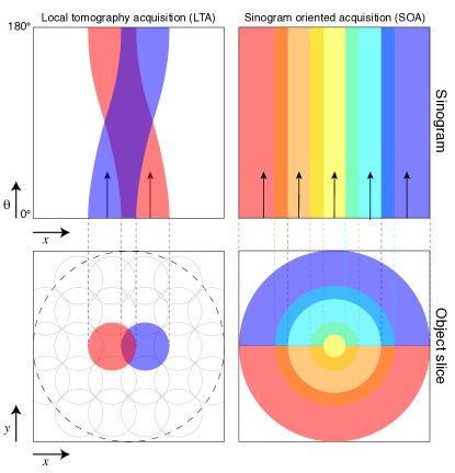
Figure 1: Comparison on the acquisition scheme of local tomography acquisition (LTA; left) versus sinogram oriented acquisition (SOA; right). The top row depicts information collection in sinogram space, where each stripe with an arrow and a distinct color represents one angular scan over $180\mathrm{°}$ (which is then used to synthesize the full $360\mathrm{°}$ sinogram). The bottom row shows the mapping of different scans to the full image of one object slice. For samples with roughly equal extension in both lateral dimensions, if the number of scans required in SOA is $n_{\textup{f}}$, then $n_{\textup{f}}^{2}$ scans are needed by LTA.

2 Methodology

2.1 Phantom object

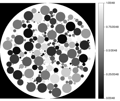
Figure 2: Phantom object created for simulations, where the highest attenuation values are white and the lowest are black. The object has a diameter, or maximum projected thickness, of $L=2048$ voxels, each set to a per-voxel linear attenuation coefficient of $\mu=1/2048$ so that the total attenuation through the disk if solid is $\exp[-1]$. The object is designed with random spherical “pores” inside with linear attenuation coefficients ranging from $\mu=0/2048$ to $\mu=1/2048$.

In order to better understand the tradeoffs between object and sinogram oriented acquisition, we created a 2D phantom sample using the open-source virtual object designing tool XDesign [15]. This represents an object slice from a 3D object. The simulated sample (Fig. 2) is a solid disk with a diameter, and thus maximum projected thickness, of $L=2048$ pixels. If solid, each pixel would be set to a linear absorption coefficient (LAC) of $\mu=1/2048$, so that its total thickness of $L=2048$ pixels would attenuate the x-ray beam by a factor of $\exp[-\mu L]=\exp[-1]$. In fact, the object was created with circular pores in its interior, with diameters ranging from 8 to 205 pixels, and linear absorption coefficients ranging from $\mu=0/2048$ (vacuum) to $\mu=1/2048$ (solid). All pores are randomly distributed with no overlapping. The object is also assumed to be fully within the depth of focus of the imaging system, with no wave propagation effects visible at the limit of spatial resolution, so that pure projection images are obtained. To generate the sinogram of the object, the Radon transform was performed using TomoPy, an open-source toolkit for x-ray tomography [16]. All tomographic reconstructions in this work are also obtained using this software package.

2.2 Sampling for LTA and SOA

To image an object larger than the imaging system’s field of view $f$, one provides some overlap between acquired projection scans. The acquisition scheme can be conveniently shown in the sinogram domain which contains both a spatial dimension and a viewing angle dimension. A scan can be represented by a band-shaped coverage on the sinogram, which is the region where we have access to the measurement. Figure 3 illustrates this coverage for SOA and LTA, respectively, with the same field-of-view size for both schemes. For LTA, a 3$\times$3 square grid is used. Brighter values in the images means that a pixel in the sinogram is sampled by the illuminating beam more frequently.

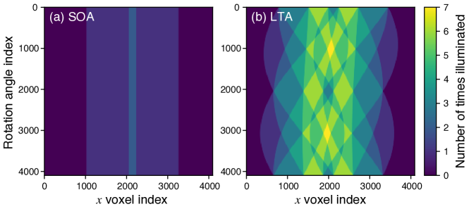
Figure 3: Coverage on the full sinogram in an experiment using (a) sinogram oriented acquisition (SOA) and (b) local tomography acquisition (LTA) with equal field-of-view. Brighter values in the images correspond to the number of times that avoxel in the object is sampled by (exposed to) the illuminating beam.

For LTA, by defining a coordination system with the origin $(0,0)$ located at the object center, it can be shown that the coverage of a local tomography scan centered at $(x,y)$ is a set of points on the $360\mathrm{°}$ synthesized sinogram given by

$$C_{\textup{LTA}}=\{(s,\theta)|s_{0}(\theta)-f/2\leq s\leq s_{0}(\theta)+f/2\}$$ (1)

with

$$s_{0}(\theta)=\sqrt{x^{2}+y^{2}}\,\cos(\alpha-\theta)+c_{0}$$ (2)

where $s$ and $\theta$ are respectively the horizontal (spatial) and vertical (angular) coordinates of the sinogram, $\alpha=\arctan(x/y)$, and $c_{0}$ is the rotation center of the synthesized $360\mathrm{°}$ sinogram. This represents a partial sinogram of the entire object, as shown in Fig. 1. For SOA, the coverage is simply a straight band extending through the angular axis. Mathematically, it can be expressed as

$$C_{\textup{SOA}}=\{(s,\theta)|p-f/2\leq s\leq p+f/2\}$$ (3)

where $p$ is the center position of the field-of-view.

For object stitching (LTA), the partial sinograms are padded with their edge values for twice their width on both sides in order to reduce boundary artifacts in the reconstruction images [12]. After reconstructing all partial sinograms, the reconstructed disks are then stitched together to form the complete reconstruction.

Since both SOA and LTA involve multiple scans, we define a quantity $n_{\textup{f}}$ that represents the number of scans along one side of the object that is required to fully reconstruct one slice of the sample. For SOA, $n_{\textup{f,PS}}$ is equal to the total number of scans; for LTA, the total number of scans is roughly $n_{\textup{f,OS}}^{2}$ considering a square grid of regions of interest (ROIs), though the actual number can vary depending on the object shape. For example, applying LTA on a thin sheet-like sample only requires roughly the same number of scans as SOA. Also, one could choose hexagonal grids which are more efficient by a factor of $\sqrt{3}$ than a square grid [17], but we assume square grids here for simplicity.

In order to fully reconstruct one slice of the object using SOA, there should be a sufficient number $n_{\textup{f,PS}}$ of scan fields to guarantee that the composite field of view completely covers the longest lateral projection of that slice. In practice, an overlap that takes a fraction $\gamma_{\rm PS}$ of the field of view between each pair of adjacent scans is needed for an automated algorithm to determine the offset between them. With this taken into account, $n_{\textup{f,PS}}$ can be denoted as

$$n_{\textup{f,PS}}=\mbox{ceil}\Big{[}\frac{L-f}{\gamma_{\rm PS}f}+1\Big{]}$$ (4)

where the function $\mbox{ceil}(x)$ is the ceiling function that returns the smallest integer that is greater than or equal to a real number $x$. Since the overlapping area diminishes the actual sample area that a scan can cover, we introduce a “useful field of view” $f^{\prime}_{\rm PS}$ for SOA, given by $f^{\prime}_{\rm PS}=\gamma_{\rm PS}f$. For example, if a 15% overlap is deliberately created between a pair of adjacent scans, then $f^{\prime}_{\rm PS}$ will be 85% of the instrumental field-of-view. Unless otherwise noted, in this work we keep the value of $\gamma_{\rm PS}$ to be 0.85 for simulation studies.

The case for LTA differs in that the scans need to cover the object slice in two dimensions. In principle, the scans in LTA can be arranged in an arbitrary pattern that complies with the actual shape of the sample. If the sample is square, then a roughly equal number of scans $n_{\textup{f,OS}}$ is needed along both sides of the object, or $n_{\textup{f,OS}}^{2}$ scans in total. A special notice should be paid to the width of the field of view in LTA, as it might not be equal to the actual field of view of the optical system. In LTA, it has been found that the reconstructed ROI often exhibits a bowl-shaped intensity profile, with values of near-boundary pixels abnormally higher [12]. Although this can be mitigated by padding the partial sinograms, this remedy does not work effectively when the truncation ratio is very low. In such scenario, the reconstructed ROIs need to have a portion of their outer pixels removed before they can be stitched. Similar to the case of SOA, we therefore introduce a “useful field of view” $f^{\prime}_{\rm OS}$ for LTA. If we use for local tomography acquisition only the content within a disk whose radius is a fraction $\gamma_{\rm OS}$ of the original ROI, then $f^{\prime}_{\rm OS}=\gamma_{\rm OS}f$. Consequently, the required number of scans $n_{\textup{f,OS}}$ is given by

$$n_{\textup{f,OS}}=\begin{cases}1&f\geq L\\ \mbox{ceil}\Big{(}\frac{\sqrt{2}L}{\gamma_{\rm OS}f}\Big{)}&f<L\end{cases}.$$ (5)

We emphasize that $n_{\textup{f,OS}}$ is the number of scans required along one side of the sample; for a square specimen, the total number of scans needed is $n_{\textup{f,OS}}^{2}$. Eq. 5 is derived assuming the scenario indicated in Fig. 4. When $f<L$, scanned ROIs are arranged in a square grid such that each corner of the bounding square of the sample disk intersects with the border of an ROI. Also, we assume that the distance between the centers of two diagonally overlapping ROIs is $f^{\prime}_{\rm OS}$ so that all ROIs exactly cover the object seamlessly. Unless specifically indicated, the value of $\gamma_{\rm OS}$ is chosen to be 0.85 for simulation studies involved in this work.

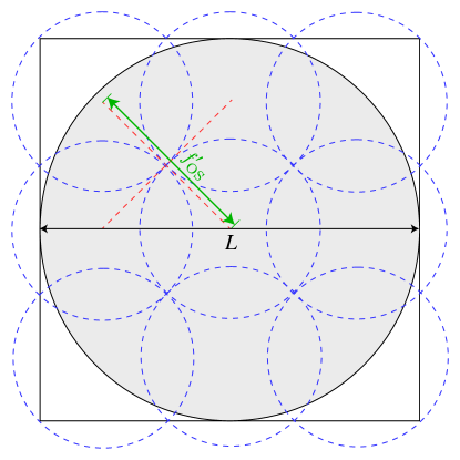
Figure 4: Schematic diagram showing the assumed pattern of data acquisition in the LTA approach of beyond-field-of-view tomography. The specimen is represented by the gray solid disk. Each local ROI that can be reconstructed using the data acquired from a scan in LTA is shown by a dashed blue circle. Each of these ROIs has a diameter of $f^{\prime}_{\rm OS}$, and they are packed in a way that the distance between the centers of each pair of diagonally adjacent ROIs is exactly $f^{\prime}_{\rm OS}$, so that the sample can be fully covered without gaps.

In order to understand the consequences of different object diameters $L$, we follow previous work [12] and characterize them in terms of a truncation ratio $T$ of

$$T=\frac{f^{\prime}}{L}$$ (6)

where of course one uses $f^{\prime}_{\rm OS}$ for local tomography acquisition (LTA) and $f^{\prime}_{\rm PS}$ for sinogram oriented acquisition (SOA).

The numerical studies in this work, which involve the simulation of data acquisition and reconstruction using both LTA and SOA, were performed using a Python package we developed called “Tomosim,” which has been made freely available on Github (https://github.com/mdw771/tomosim). The charcoal tomographic dataset has been made available on TomoBank [18] with a sample ID of 00078.

2.3 Radiation dose calculation

The differential energy deposition $dE$ within an infinitesimal depth $dt$ is formulated from the Lambert-Beer law as

$$\frac{dE}{dt}=\Big{|}\bar{n}E_{0}\frac{dI}{dt}\Big{|}$$ (7)

where $\bar{n}$ is the average number of incident photons per voxel, and $E_{0}$ is the photon energy. The Lambert-Beer law gives $\mu_{\boldsymbol{r}}(t)$, the x-ray LAC of the sample as a function of penetration depth $t$ along the current transmission direction $\boldsymbol{r}$, as $\mu_{\boldsymbol{r}}(t)=-[1/I(t)](dI/dt)$. To simplify our later computation with this term included in an integral with regards to $t$, we approximate the quantity $I(t)$ in the factor prior to $dI/dt$ as $I(t)\approx I(L/2)=\exp(-\bar{\mu}L/2)$, where $\bar{\mu}$ is the mean LAC of the specimen. Equation 7 then becomes

$$\frac{dE}{dt}=\bar{n}E_{0}\exp(-\bar{\mu}L/2)\mu_{\boldsymbol{r}}(t).$$ (8)

Again, the term $\exp(-\bar{\mu}L/2)$ represents the beam attenuation factor at the center of the object, but it can also be used to approximate the average normalized beam intensity “seen” by an arbitrary voxel of the object in one viewing direction. Accordingly, we also replace $\mu_{\boldsymbol{r}}(t)$ in Eq. 8 with a constant value of $\bar{\mu}$. This approximation is valid as long as the LAC of the object varies slowly. By integrating both sides over the voxel size $\Delta$, we obtain the energy absorbed by this voxel as

$$E=\bar{n}E_{0}\exp(-\bar{\mu}L/2)\bar{\mu}\Delta.$$ (9)

Then, the radiation dose received by this $j$-th voxel per ($180\mathrm{°}$) scan is given by

$$D_{s,j}=\frac{N_{\theta}\bar{n}E_{0}\exp(-\bar{\mu}L/2)\bar{\mu}}{\rho\Delta^{2}}$$ (10)

where $N_{\theta}$ is the number of projection angles, and $\rho$ is the object density. The subscript $s$ in $D_{s,j}$ denotes the $s$-th scan. Again, for SOA, a total of $n_{\textup{f,PS}}$ scans are needed, while for LTA the number is on the order of $n_{\textup{f,OS}}^{2}$. Based on this, one can estimate the total radiation dose received by the sample by summing up the number of occasions of being exposed to the beam over all voxels ($j$) and all scans ($s$). This is compactly expressed as

$$D = \sum_{s}\sum_{j}D_{s,j}$$ (11)

$$\propto \sum_{s}\epsilon\Omega_{s}$$

where $\Omega_{s}$ is the total area in sinogram domain that is sampled in one scan (which is equal to the width in pixels of a field of view multiplied by the number of projection angles), and $\epsilon$ is the fraction of pixels where the sample is present (i.e., pixels that are not purely air).

2.4 Experimental data acquisition and registration

For an experimental tests on sinogram oriented acquisition (SOA), we used experimental data collected using 25 keV X rays at beamline 32-ID of the Advanced Photon Source at the Argonne National Laboratory. The specimen is a truncated charcoal sample with a diameter of $d=4$ mm, whereas the imaging system field of view was $f=1920\times 0.6$ $\mu$m=1.12 mm. With $\gamma_{\rm PS}=0.9$, this yields a reduced field of view of $f^{\prime}_{\rm PS}=1.04$ mm so that $n_{\textup{f,PS}}=4$ and $T=0.26$. Registration of the sinograms was done using phase correlation, which can be formulated as

$$\boldsymbol{c}=\operatorname*{argmax}_{x\in\mathbb{R}^{2}}\mathcal{F}^{-1}\Bigg{[}\frac{\mathcal{F}[I_{a}(\boldsymbol{x})]\mathcal{F}[I^{*}_{b}(\boldsymbol{x})]}{|\mathcal{F}[I_{a}(\boldsymbol{x})]\mathcal{F}[I^{*}_{b}(\boldsymbol{x})]|}\Bigg{]}(\boldsymbol{x}).$$ (12)

This method is reliable when a large number of high-contrast features are present in the overlapping region of both images $I_{a}$ and $I_{b}$, and when noises are not heavily present. In practice, photon flux ($\bar{n}$ in Eq. 10) sometimes needs to be reduced in order to lower the radiation dose imposed on the sample. This can lead to higher photon noise that challenges image registration.

3 Results and discussion

3.1 Comparison on dose-efficiency

As one can easily see from Fig. 1, object stitching (LTA) requires a larger number of scans than sinogram oriented acquisition (SOA) by a factor of about $1/T$. Because much of the illumination of one scan goes into out-of-local-tomogram regions in local tomography acquisition, this also means that the object is exposed to a higher radiation dose. In Eq. 11, the total radiation dose of an experiment is shown to be approximately proportional to the area of non-air regions sampled in the sinogram, given that the sample does not contain large fluctuations in absorption coefficient. In this equation, $\Omega_{s}$ itself is also an interesting quantity to investigate. The sum of the areas of all $\Omega_{s}$ regions in the sinogram, which also includes those “air” pixels, provides an intuitive measurement of the acquired data size, which is jointly determined by the actual field of view, the number of scans $s$, and the number of projection angles $N_{\theta}$. For a given experimental configuration, this summed area is denoted by $A$. A lower $A$ means that the sample can be entirely imaged and reconstructed with a smaller data size (i.e., less disk space is needed to store a complete acquisition), which is desirable in the case where only limited storage and computing resources are available.

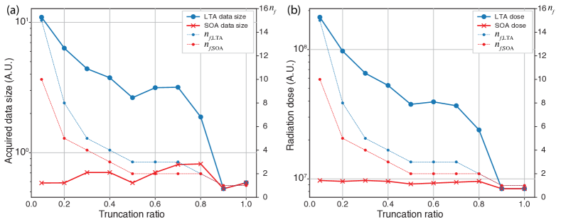
Figure 5: Acquired data size (a) and radiation dose (b) as a function of the truncation ratio $T$ of Eq. 6 for both local tomography acquisition (LTA) and sinogram oriented acquisition (SOA). In each subplot, the variation of $n_{\textup{f,PS}}$ and $n_{\textup{f,OS}}$ is also shown. The figure indicates that the acquired data size and radiation dose do not necessarily decrease with increasing truncation ratio; rather, both quantities are associated with the arrangement of scans in an actual experiment. These results were calculated for fixed values of $\gamma_{\rm PS}=0.85$ and $\gamma_{\rm OS}=0.85$ as discussed in the text.

With these quantities defined, Fig. 5(a) shows the results for acquired data size $A_{\textup{SOA}}$ and $A_{\textup{LTA}}$ as a function of truncation ratio $T$ , while Fig. 5(b) shows $D_{\textup{SOA}}$ and $D_{\textup{LTA}}$. The dashed lines in each plot show the variation of $n_{\textup{f,PS}}$ and $n_{\textup{f,OS}}$. Note that $n_{\textup{f,OS}}$ is the number of scans along one side of the object, so that $n_{\textup{f,OS}}^{2}$ scans are required for local tomography acquisition (LTA). When examining this figure, it has to be noted that no matter what $T$ is, the values of $\gamma_{\rm PS}$ and $\gamma_{\rm OS}$ are fixed. This means that area covered by all scans in either SOA or LTA might be larger than the sample. In such cases, we allow acquisition to extend beyond the right side of the sample for SOA; for LTA, the exceeded margins are on the right and and bottom sides of the sample. The “overflow” of acquisition does not substantially affect $D$, but can increase $A$. It can be seen in Fig. 5(a) that $A$ is not a monotonic function of $T$, although it does show an overall decreasing trend with increasing $T$. For example, when $T$ grows from 0.5 to 0.7, $A_{\textup{LTA}}$ increases while $n_{\textup{f,OS}}$ is unchanged. This is explained by the larger “overflow” of scanned field beyond the actual object. In contrast, the increase in $T$ that does not cause a reduction of $n_{\textup{f}}$ only results in a small cost of $D$ due to the increase of overlapping areas required between adjacent scans. However, the overall observation is still that SOA is both more data-efficient and dose-efficient than LTA in general. The figures indicate that no matter which method is used, a higher $T$ does not necessarily imply better data efficiency in the case of $f<L$. One should thus carefully choose the camera to use in order to optimize the experiment in terms of both data size and radiation dose.

3.2 Comparison on reconstruction artifacts

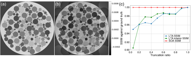
Figure 6: Comparison of image quality between local tomography acquisition (LTA) and sinogram oriented acquisition (SOA). This comparison is made using the Structural SIMilarity index (SSIM) with regards to the ground truth image, against reconstructions for SOA (a) and LTA (b). When noise is not a factor, and registration errors are negligible, the SOA result is identical to the ground truth. Also shown (c) is the SSIM as a function of truncation ratio $T$.

While both LTA and SOA are subject to photon noise during measurement, other types of artifacts can also participate in determining the reconstruction quality. The sources of noise and artifacts in the final reconstructions for SOA are straightforward to understand. In particular, when the intensity of adjacent projection tiles differs, ring artifacts can be seen in the reconstruction if the sinograms are not properly blended where they overlap. For LTA, reconstruction quality is mainly affected by three factors other than noise in the raw data. First, since the illuminating beam at different scan positions and illumination angles arrive at the object region with varying transmission through out-of-object-field features, the overall intensity of the reconstruction disk can vary between neighboring tiles. This issue can be mitigated by gradient-based image blending techniques such as Poisson blending [19], but they are usually time-consuming and are not appropriate when the number of tiles is large. Second, a bowl-shaped intensity profile across an individual reconstruction disk is often observed in ROI tomography, in which case the pixel intensities near the edge of the reconstruction disk are shifted higher. This can be alleviated by padding the partial sinograms on its left and right sides (along the spatial axis) by the edge values [12]. In our case, the sinograms were padded by twice their length on each side, but this did not completely eliminate distortion in the intensity profile. Finally, each projection image collected inevitably contains information of the portion object lying outside of the ROI, which, at least to some minor extent, violates the Fourier slice theorem [20]. When the truncation ratio is not too low, one can use this excessive information to slightly expand the field-of-view by padding both sides of the sinogram with its edge values; however, streak artifacts will be heavily present in the area out of the scanned disk in the case of a small truncation ratio [13]. In addition, ideally, one would also seek to satisfy the Crowther criterion [21] on the required number of rotation angles based on the entire object size rather than the size of the local tomography region of interest. One can thus expect aliasing artifacts especially for low truncation ratios.

To quantify the reconstruction quality, we used Structural SIMilarity (SSIM; [22]) as a metric for the fidelity of the stitched reconstruction images with regards to the ground truth image. The SSIM allows us to independently examine the structural fidelity of an image with regards to the reference by incorporating the inter-dependency of image pixels, especially when they are spatially close. These dependencies carry important information about the structure, so that it serves as an accurate and reliable tool for evaluation. The reconstruction images were obtained by applying filtered backprojection (FBP) algorithm to the full-object sinogram. SSIM is defined as a product of three terms that assess the similarity between two images $A$ and $B$ in different aspects. These include the luminance ($l$), the contrast ($c$), and the structure ($s$), defined by

$$l(A,B) = \frac{2\mu_{A}\mu_{B}+c_{1}}{\mu_{A}^{2}+\mu_{B}^{2}+c_{1}}$$ (13)

$$c(A,B) = \frac{2\sigma_{A}\sigma_{B}+c_{2}}{\sigma_{A}^{2}+\sigma_{B}^{2}+c_{2}}$$ (14)

$$s(A,B) = \frac{\sigma_{AB}+c_{3}}{\sigma_{A}\sigma_{B}+c_{3}}$$ (15)

where

$$c_{1} = (k_{1}L)^{2}$$ (16)

$$c_{2} = (k_{2}L)^{2}$$ (17)

$$c_{3} = c_{2}/2$$ (18)

with typical values of $k_{1}$ and $k_{2}$ set to 0.01 and 0.03, and $L$ being the dynamic range of the grayscale images. In Eqs. 13 to 15, $\mu_{i}$ and $\sigma_{i}$ represent the mean and standard deviation of image $i$ ($i=A$ or $B$), and $\sigma_{AB}$ is the covariance of image $A$ and $B$ [22]. While it is common to calculate the SSIM as the product of all three terms, we set $l(A,B)=1$ here in order to exclude the overall intensity shifting and scaling. Thus for all quality evaluations in this work, we have

$$\mbox{SSIM}(A,B)=c(A,B)\cdot s(A,B).$$ (19)

Figs. 6(a) and (b) respectively show the stitched reconstructions obtained from SOA and LTA with $T=0.2$. If the beam brightness is sufficiently high and stable, then noise and intensity variations between adjacent tiles can be neglected. In this case, the stitched sinogram in SOA is not affected by other systematic artifacts, and is identical to the full-object sinogram. However, the stitched reconstruction in LTA is affected by intensity variations and bowl-profile artifacts, even though the partial sinograms were padded before reconstruction and only the inner $\gamma_{\rm OS}=0.85$ of the reconstructed ROIs were used. Fig. 6 plots the SSIM of the reconstructed porous disk (vacuum portions at the corners are not included) with regards to the ground truth for both two approaches. As can be seen, the quality of the SOA reconstruction is in principle not affected by the truncation ratio. In contrast, an overall reduction in SSIM with decreasing truncation ratio is seen for LTA. In order to examine how the truncation ratio $T$ influences the reconstruction quality of an individual reconstruction disk in LTA, we also computed the mean SSIM of the inner portions in all reconstructed ROIs that are far from the boundaries and termed it the “LTA interior SSIM” in Fig. 6. In this way, the influence of the bowl-profile artifacts can be excluded. As in Fig. 6, this SSIM also drops with diminishing $T$. This indicates that in addition to boundary artifacts, a low truncation ratio also deteriorates the intrinsic reconstruction quality of the ROI, which is mainly in the form of noise caused by out-of-ROI information.

3.3 Comparison on image registration feasibility

Registration refers to the processing of finding the relative positional offset between adjacent tiles in mosaic tomography. For SOA, registration is done in projection domain before merging the partial datasets. LTA, on the other hand, involves registration on reconstructed images. The large number of tiles in mosaic tomography poses huge difficulties for manual registration, and automatic registration methods are usually employed. Phase correlation (PC) is the most popular registration algorithm, where the offset vector $\vec{c}$ between two images $I_{a}$ and $I_{b}$ is determined by

$$\vec{c}=\operatorname*{argmax}\Bigg{(}\mathcal{F}^{-1}\Bigg{[}\frac{\mathcal{F}[I_{a}(\vec{x})]\mathcal{F}[I^{*}_{b}(\vec{x})]}{|\mathcal{F}[I_{a}(\vec{x})]\mathcal{F}[I^{*}_{b}(\vec{x})]|}\Bigg{]}(\vec{x})\Bigg{)}.$$ (20)

In Eq. 20, $\mathcal{F}$ is the Fourier transform operator, and $I^{*}_{i}$ represents the complex conjugate of $I_{i}$.

The transmission radiographs for specimens that are thick and not entirely periodic generally do not exhibit a good number of distinguishable fine features, because the features tend to entangle and blend into each other when they are superposed along the beam path. However, this does not imply that SOA projections are intrinsically harder objects for registration compared to LTA reconstructions. Although it is conceptually plausible that more high-frequency features arise in reconstructed images, we should notice that phase correlation is a technique that is susceptible to noise. When data are collected with low photon flux, Poisson noise is more pronounced, and tomographic reconstructions based on the Fourier slice theorem can be more heavily affected by noise due to the amplification of high-frequency artifacts by the ramp filter [20] (though this issue can be mitigated by adding a Weiner filter). To investigate the photon noise sensitivity of alignment, we carried out the following numerical study. We created a projection panorama of our whole charcoal specimen, and extracted a row of $1024\times 1024$ pixel tiles from it with a constant interval of 850 pixels. As the projection panorama was normalized using the dark field and white field data, all tiles extracted contain pixels with values ranging between 0 and 1. Here we denote the image by $I$. We then define a scaling factor $n_{\rm ph}$ to represent a “mean” photon count for each pixel. In other words, $n_{\rm ph}$ is the number of photons incident on a pixel of the acquired radiograph. Poisson noises was subsequently applied to all tiles, using the probably density function of

$$f(k,n_{\rm ph}I)=\frac{(n_{\rm ph}I)^{k}e^{-n_{\rm ph}I}}{k!}$$ (21)

where $k$ is the actual number of photon count. The noisy version of the tiles were then pre-processed by taking their negative logarithm, and registered using phase correlation. For LTA, different levels of Poisson noise were added to extracted partial sinograms, from which reconstruction images were subsequently created and registered. The field of view in this case is 1024 pixels. Since data fidelity is guaranteed only within a disk for an LTA reconstruction, we use a smaller offset of 700 pixels in both the $x$ and $y$ directions in order to compensate the smaller usable overlapping area. Figure 7(a) compares the registration accuracy of LTA and SOA over a range of photon budgets per pixel, which is the total number of photons to be applied to a specimen voxel during the experiment. Thus, all comparisons between LTA and SOA are based on the condition that the total radiation doses are equal. The photon budget is evenly distributed to all scans and $n_{\rm ph}$ is calculated accordingly, in which case LTA will have a lower $n_{\rm ph}$ in a single scan compared to SOA. For our test data, the mean registration error of SOA is always below 1, while LTA requires a photon budget of about 2000 for the mean error to diminish into the sub-pixel level.

The number of projection angles can also impact the registration accuracy for LTA since it is done in the reconstruction domain. In Fig. 7(b), the mean registration error is plotted with regards to the level of downsampling in the axis of projection angles. The original data involve 4500 projections, which were downsampled by factors of powers of 2. The result indicates that the error starts to exceed the pixel-level boundary when the downsampling level is larger than 4.

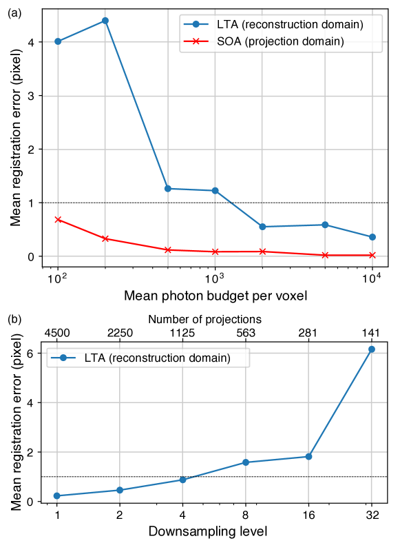
Figure 7: Mean registration error plotted against (a) the average photon budget per voxel for both SOA and LTA, and (b) the downsampling level in projection angles for LTA. The plot indicates that the accuracy of phase correlation degrades when projection images become more noisy due to lower number of incident photons. For this particular sample, registration in reconstruction domain for LTA requires a higher incident photon flux in order to give reliable registration results. In addition, a reduction in projection angles also causes a significant deterioration in registration accuracy for LTA.

A critical drawback of SOA is that registration errors are accumulative, which means that deviations in the offset determined for any pair of tiles can affect the quality of a large part or even the entirety of the final reconstruction. On the other hand, registration errors in LTA involve multiple tiles intersecting on several sides, giving less opportunity for alignment pathologies along one edge to dominate global alignment. For SOA, the accumulated registration error throughout a row in the tile grid would cause the relative center of rotation to deviate from the true value for tiles that are far away from the rotation axis. Since the reconstruction of SOA takes the registration results as an input, this can lead to off-center distortions on small features at some locations of the full reconstruction. To show this, we compare the reconstructions for a part of the data collected from our charcoal sample. To simulate the SOA result with induced error, we extracted 8 tiles from the full sinogram with a fixed interval of 795 pixels. The registered positions of all tiles were then deliberately adjusted by errors following a Gaussian distribution with a standard deviation of 4, after which they were stitched and reconstructed. The center of rotation set for the reconstructor was determined to optimize the reconstruction quality of the central region of the sample. The LTA results serving as a reference were obtained by extracting partial sinograms from the full sinogram, and then reconstructing them individually. Using these procedures, we show in Fig. 8 a comparison of two local regions of the reconstructions obtained using SOA and LTA, respectively. One of these regions is exactly at the object center, while the other one is around 1000 pixels above in the object slice view. The positions of both regions are marked on the full reconstruction slice. For the central region (shown in the second row of the image grid in Fig. 8), the exhibited images have nearly the same quality. However, for the off-center region, some dot-shaped features extracted from the SOA reconstruction become heavily distorted (as marked by the colored arrows in the SOA figure on the first row of the grid). This indicates an erroneous registration outcome for the tile contributing to this region, which deviates the distance of the projections contained in this tile to the rotation center away from the accurate value. When the tiles are correctly registered, as shown in the inset of the SOA figure, the distortion no longer exists.

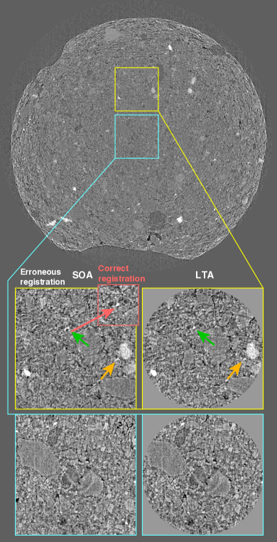
Figure 8: Comparison of the effect of registration errors. Shown here are sinogram oriented acquisition (SOA; left column in the grid) and local tomography acquisition (LTA; right column) reconstructions at an region-of-interest (first row) and the center (second row) of a slice in the charcoal sample. The SOA reconstruction was done by stitching 8 tiles extracted from the full sinogram. Registration errors following a Gaussian distribution with a standard deviation of 4.0 were exerted to the tile positions before stitching. The rotation centerfor SOA reconstruction was calibrated to optimize the quality around the object center. As a result, the central region of the charcoal reconstructed using both methods appears similar. However, at around 1000 pixels above the object center, the SOA reconstruction shows severe distortion of dot-features (pointed by colored arrows) due to the deviation of its actual position from the rotation center inputted to the reconstruction routine. The inset in the SOA figure shows the appearance of one of the distorted features when the tiles are correctly registered.

Local tomography acquisition (LTA) reconstructions are not globally affected by registration errors. We further note that in addition to this feature, LTA is advantageous compared to SOA in several other aspects. For certain sample geometries, LTA can achieve better dose efficiency than SOA by using more projection angles for highly interesting regions of the sample while using fewer angles for the rest. Also, LTA allows one to flexibly select reconstruction methods or parameters for different ROIs. For example, an ROI where features lie in textured backgrounds can be reconstructed using Bayesian methods with stronger sparsity regularization in order to suppress background structures.

4 Conclusion

We have compared two methods for tomography of objects that extend beyond the field of view of the illumination system and camera, based on their radiation dose, reconstruction fidelity, and the presence of registration artifacts. Sinogram oriented acquisition (SOA) gives lower radiation dose, and it is also generally free of inter-tile intensity variations, in-tile intensity “bowl” artifacts, and noise induced by out-of-local-tomogram information. In addition, tile registration is shown to be no harder than with Local tomography acquisition (LTA), especially when the noise level is high. The major drawback of SOA is that registration errors are accumulative and can affect the entire reconstruction. Our present efforts are directed towards providing more reliable registration algorithms in order to improve the reconstruction quality of SOA for thick amorphous samples; one approach that offers promise is iterative reprojection [23, 24, 25], though it will be computationally demanding for large datasets.

5 Acknowledgement

This research used resources of the Advanced Photon Source and the Argonne Leadership Computing Facility, which are U.S. Department of Energy (DOE) Office of Science User Facilities operated for the DOE Office of Science by Argonne National Laboratory under Contract No. DE-AC02-06CH11357. We thank the National Institute of Mental Health, National Institutes of Health, for support under grant U01 MH109100. We also thank Vincent De Andrade for his help with acquiring the data on the charcoal sample shown in the paper.

References

- [1] Kyrieleis, A., Ibison, M., Titarenko, V. & Withers, P. J. Image stitching strategies for tomographic imaging of large objects at high resolution at synchrotron sources. Nuclear Instruments and Methods in Physics Research A 607, 677–684 (2009).
- [2] Kuchment, P., Lancaster, K. & Mogilevskaya, L. On local tomography. Inverse Problems 11, 571–589 (1995).
- [3] Lewitt, R. M. & Bates, R. H. T. Image reconstruction from projections: I: General theoretical considerations. Optik 50, 19–33 (1978).
- [4] Natterer, F. The Mathematics of Computerized Tomography (John Wiley & Sons, Chichester, 1986).
- [5] Oikonomidis, I. V. & Lovric, G. Imaging samples larger than the field of view: the SLS experience. Journal of Physics: Conference Series 849, 012004 (2017).
- [6] Vescovi, R. F. C., Cardoso, M. B. & Miqueles, E. X. Radiography registration for mosaic tomography. Journal of Synchrotron Radiation 24, 686–694 (2017).
- [7] Sztrókay, A. et al. High-resolution breast tomography at high energy: a feasibility study of phase contrast imaging on a whole breast. Physics in Medicine and Biology 57, 2931–2942 (2012).
- [8] Liu, Y. et al. TXM-Wizard: a program for advanced data collection and evaluation in full-field transmission x-ray microscopy. Journal of Synchrotron Radiation 19, 281–287 (2012).
- [9] Mokso, R. et al. X-ray mosaic nanotomography of large microorganisms. Journal of Structural Biology 177, 233–238 (2012).
- [10] Kalender, W. A. Technical foundations of spiral CT. Seminars in Ultrasound, CT and MRI 15, 81–89 (1994).
- [11] Pelt, D. M. & Parkinson, D. Y. Ring artifact reduction in synchrotron x-ray tomography through helical acquisition. Measurement Science and Technology 29, 034002–10 (2018).
- [12] Kyrieleis, A., Titarenko, V., Ibison, M., Connolley, T. & Withers, P. J. Region-of-interest tomography using filtered backprojection: assessing the practical limits. Journal of Microscopy 241, 69–82 (2010).
- [13] da Silva, J. C. et al. Quantitative region-of-interest tomography using variable field of view. Opt Express 26, 16752–16768 (2018).
- [14] Reimer, L. & Schmidt, A. The shrinkage of bulk polymers by radiation damage in an SEM. Scanning 7, 47–53 (2011).
- [15] Ching, D. J. & Gürsoy, D. XDesign: an open-source software package for designing x-ray imaging phantoms and experiments. Journal of Synchrotron Radiation 24, 537–544 (2017).
- [16] Gürsoy, D., De Carlo, F., Xiao, X. & Jacobsen, C. TomoPy: a framework for the analysis of synchrotron tomographic data. Journal of Synchrotron Radiation 21, 1188–1193 (2014).
- [17] Heinzer, S. et al. Hierarchical microimaging for multiscale analysis of large vascular networks. NeuroImage 32, 626–636 (2006).
- [18] De Carlo, F. et al. TomoBank: a tomographic data repository for computational x-ray science. Measurement Science and Technology 29, 034004 (2018).
- [19] Perez, P., Gangnet, M. & 0001, A. B. Poisson image editing. ACM Transactions on Graphics 22, 313 (2003).
- [20] Kak, A. C. & Slaney, M. Principles of Computerized Tomographic Imaging (Society for Industrial and Applied Mathematics, 2012).
- [21] Crowther, R. A., DeRosier, D. J. & Klug, A. The reconstruction of a three-dimensional structure from projections and its application to electron microscopy. Proceedings of the Royal Society of London A 317, 319–340 (1970).
- [22] Wang, Z., Bovik, A. C., Sheikh, H. R. & Simoncelli, E. P. Image quality assessment: From error visibility to structural similarity. IEEE Transactions on Image Processing 13, 600–612 (2004).
- [23] Dengler, J. A multi-resolution approach to the 3D reconstruction from an electron microscope tilt series solving the alignment problem without gold particles. Ultramicroscopy 30, 337–348 (1989).
- [24] Latham, S. J., Kingston, A. M., Recur, B., Myers, G. R. & Sheppard, A. P. Multi-resolution radiograph alignment for motion correction in x-ray micro-tomography. Proceedings SPIE 9967, 996710 (2016).
- [25] Gürsoy, D. et al. Rapid alignment of nanotomography data using joint iterative reconstruction and reprojection. Scientific Reports 7, 11818 (2017).