RELICS: A Strong Lens Model for SPT-CLJ06155746, a Cluster
Abstract
We present a lens model for the cluster SPT-CLJ06155746, which is the highest redshift () system in the Reionization of Lensing Clusters Survey (RELICS), making it the highest redshift cluster for which a full strong lens model is published. We identify three systems of multiply-imaged lensed galaxies, two of which we spectroscopically confirm at and , which we use as constraints for the model. We find a foreground structure at , which we include as a second cluster-sized halo in one of our models; however two different statistical tests find the best-fit model consists of one cluster-sized halo combined with three individually optimized galaxy-sized halos, as well as contributions from the cluster galaxies themselves. We find the total projected mass density within (the region where the strong lensing constraints exist) to be M☉. If we extrapolate out to , our projected mass density is consistent with the mass inferred from weak lensing and from the Sunyaev-Zel’dovich effect ( M☉). This cluster is lensing a previously reported galaxy, which, if spectroscopically confirmed, will be the highest-redshift strongly lensed galaxy known.
1 Introduction
Gravitational lensing occurs when light from a background object is deflected around mass between the object and the observer. The amount of deflection is related to the strength of the gravitational field; i.e., the mass distribution, as well as to the geometrical configuration of the lens, source, and observer. The deflection is independent of the type of matter and its state, meaning that lensing is sensitive to both luminous and dark matter. Thus, it is ideal for measuring the projected mass density of the cluster core to great precision out to the location of the strong lensing constraints. Nevertheless, strong and weak lensing measurements of mass and lensing magnifications are prone to systematic uncertainties (Johnson & Sharon, 2016; Meneghetti et al., 2017). Most notably, it is sensitive to structure along the line of sight (e.g., D’Aloisio & Natarajan, 2011; Bayliss et al., 2014; Jaroszynski & Kostrzewa-Rutkowska, 2014; McCully et al., 2017; Chirivì et al., 2017), as all matter along the line of sight contributes to the observed lensing signal.
While there are quite a few known strong lensing clusters at lower redshifts, there are only a handful at , despite the many targeted searches for high redshift clusters (Wylezalek et al., 2014; Bleem et al., 2015; Paterno-Mahler et al., 2017). For many of these high-redshift strong-lensing clusters, strongly lensed galaxies are observed in the form of stretched arcs; however no detailed lens models exist in the literature (Huang et al., 2009; Gonzalez et al., 2012). This is likely due to the difficulties in computing such models: they require a large investment of time on the Hubble Space Telescope (HST) to obtain enough constraints, as well as spectroscopic follow-up to obtain redshifts.
Mass modeling of strong gravitational lenses at a large range of redshifts allows us to test predictions about the universe. We can compare the observed distribution of lenses, lens mass, and the distribution of the brightness of lensed galaxies (among other properties) to simulations for varying cosmological parameters to test our theories. Such studies have been done for small cluster samples (Bartelmann et al., 1998; Wambsganss et al., 2004; Dalal et al., 2004; Ho & White, 2005; Li et al., 2005; Sand et al., 2005; Hennawi et al., 2007; Horesh et al., 2011; Bayliss et al., 2011; Xu et al., 2016).
Here we present a strong lens model for the cluster SPT-CLJ06155746 (also known as PLCKG266.627.3; hereafter SPT0615; RA: 06h15m56s, DEC: ; Planck Collaboration et al., 2011; Williamson et al., 2011; Bleem et al., 2015). This is the highest redshift cluster in the Reionization of Lensing Clusters Survey (RELICS) sample, with (Planck Collaboration et al., 2016). The study of lensing clusters in the regime is crucial to understanding the statistics described above, as some of the lensed galaxies behind high-redshift lensing clusters should not exist due to their brightness, based on current realistic assumptions (Gonzalez et al., 2012). A statistical sample of high-redshift lensing clusters give us the ability to understand the true frequency of lensed galaxies behind high-redshift clusters.
The goal of the RELICS project is to find a statistically significant sample of galaxies at high redshift to constrain the luminosity function at (Salmon et al., 2017) and probe the epoch of reionization at (Salmon et al., 2018). RELICS uses gravitational lensing by galaxy clusters to search for these magnified high-redshift galaxies; secondary science goals include cluster physics (such as mass scaling relations) and discovering supernovae. Archival HST imaging reveals that SPT0615 is a strong lensing cluster. The primary lensing evidence comes from a source galaxy nearly directly behind the cluster is strongly lensed into three images, which are the most notable strong lensing constraints in the field. We use these, along with other newly discovered lensed galaxies and their spectroscopic redshifts, to determine a strong lensing mass model of SPT0615.
This paper is organized as follows: in §2 we present the data from the various observatories used and in §3 we present our modeling efforts. In §4 we discuss the results of our modeling and compare our results to other high-redshift clusters that also have strong lens models. Throughout this work we assume a flat cosmology with km s-1 Mpc-1, , and . At the redshift of SPT0615 (), this gives a scale of kpc and a luminosity distance of Mpc.
2 Data and Data Reduction
2.1 HST Imaging
SPT0615 was observed with HST as part of the Reionization of Lensing Clusters Survey (RELICS, GO-14096, PI: Coe) Treasury HST program, which aimed to discover a statistically significant samples of galaxies at high redshift (, Salmon et al., 2017). The cluster selection process is described in detail in Cerny et al. (2017) and Coe et al. (in prep), and strong lensing analyses for other RELICS clusters were published in Cerny et al. (2017), Acebron et al. (2018), and Cibirka et al. (2018). SPT0615 was observed for two orbits with the Wide Field Camera 3 (WFC3) in F105W, F125W, F140W, F160W and for one orbit with the Advanced Camera for Survey (ACS) in F435W. All clusters in the program were imaged over two epochs to allow for variability searches. Additional archival ACS imaging in F606W and F814W were available from GO-12757 (PI: High) and GO-12477 (PI: Mazzotta). GO-12477 obtained one pointing of F814W imaging and a mosaic in F606W. GO-12757 obtained a mosaic in F814W, including overlapping area for deeper imaging in the strong lensing region. The center of the field will have a deeper limiting magnitude. The wavelength coverage spans µm. Table 1 summarizes the observations.
Calibrated images from all available programs, including archival programs, were obtained from the Mikulski Archive for Space Telescopes (MAST)111https://archive.stsci.edu. Individual frames were then visually inspected to ensure that the quality is acceptable for science. Satellite trails and other image artifacts were manually masked out. Additionally, the WFC3/IR images have persistence which was masked out using products supplied by the WFC3 team. A custom pixel mask provided by G. Brammer (personal communication) removes hot pixels not in the pipeline mask. The ACS images were corrected for charge transfer inefficiency losses using the method described in Anderson & Bedin (2010). Sub-exposures in each filter were combined to form a deep image using the AstroDrizzle package (Gonzaga & et al., 2012) using PIXFRAC. The images in different filters were aligned to the same reference frame, and the astrometry was matched to the Wide-field Infrared Survey Explorer (WISE) point source catalog (Wright et al., 2010). The final, reduced images are made available to the public as high level science products through MAST222https://archive.stsci.edu/prepds/relics. The public release includes photometric catalogs of all the fields, including photometric redshift estimates using the Bayesian Photometric Redshifts method (BPZ; Benítez, 2000).
| Instrument | Exp. Time (s) | UT Date | Program |
|---|---|---|---|
| ACS/WFC F435W | 2249 | 2017-02-08 | GO14096aaRELICS program |
| ACS/WFC F606W | 1920 | 2012-01-20 | GO12477bbThese images are different pointings of a mosaic. |
| ACS/WFC F606W | 1920 | 2012-01-20 | GO12477bbThese images are different pointings of a mosaic. |
| ACS/WFC F606W | 1920 | 2012-01-21 | GO12477bbThese images are different pointings of a mosaic. |
| ACS/WFC F606W | 1920 | 2012-01-21 | GO12477bbThese images are different pointings of a mosaic. |
| ACS/WFC F814W | 2476 | 2012-01-19 | GO12757bbThese images are different pointings of a mosaic. |
| ACS/WFC F814W | 2476 | 2012-01-19 | GO12757bbThese images are different pointings of a mosaic. |
| ACS/WFC F814W | 1916 | 2012-01-21 | GO12477 |
| ACS/WFC F814W | 2476 | 2012-01-22 | GO12757bbThese images are different pointings of a mosaic. |
| ACS/WFC F814W | 2476 | 2012-01-25 | GO12757bbThese images are different pointings of a mosaic. |
| WFC3/IR F105W | 755.9 | 2017-02-08 | GO14096aaRELICS program |
| WFC3/IR F105W | 755.9 | 2017-03-23 | GO14096aaRELICS program |
| WFC3/IR F125W | 380.9 | 2017-02-08 | GO14096aaRELICS program |
| WFC3/IR F125W | 380.9 | 2017-03-23 | GO14096aaRELICS program |
| WFC3/IR F140W | 380.9 | 2017-02-08 | GO14096aaRELICS program |
| WFC3/IR F140W | 380.9 | 2017-03-23 | GO14096aaRELICS program |
| WFC3/IR F160W | 1055.9 | 2017-02-08 | GO14096aaRELICS program |
| WFC3/RI F160W | 1055.9 | 2017-03-23 | GO14096aaRELICS program |
2.2 Ground-Based Spectroscopy
Ground-based spectroscopic observations were obtained using the upgraded Low Dispersion Survey Spectrograph (LDSS3-C) on the Magellan Clay telescope using University of Arizona (PI: Stark) allocation. SPT0615 was observed on 2017 March 30 for a total exposure time of one hour. Average seeing was throughout the night. Slits were placed on candidate lensed galaxies. The VPH-ALL grism was used, which has coverage between . A 1″ slit was used on all objects, with spectral resolution R 450-1100 across the wavelength range. The detector is in spatial extent. A full description of the RELICS Magellan/LDSS3 followup results will be presented in a future paper (Mainali et al. in prep).
3 Lens Model
The model is computed using Lenstool (Jullo et al., 2007), which is a parametric model that uses Monte Carlo Markov Chain (MCMC) analysis to sample the parameter space. Each dark matter halo is modeled as a pseudo-isothermal ellipsoidal mass distribution (PIEMD; Limousin et al., 2005) with seven parameters: position (RA, DEC), mass (or velocity dispersion, ), ellipticity (), position angle (), core radius (), and truncation radius (). Dark matter halos are assigned to both the cluster as a whole and to individual cluster galaxies. Cluster galaxies are selected via the cluster red sequence (Gladders & Yee, 2000). The position and shape parameters of cluster galaxies are fixed to their observed properties as measured from the galaxy light using Source Extractor (Bertin & Arnouts, 1996), and their mass-to-light ratios are assigned using scaling relations (Limousin et al., 2005). The parameters for the cluster halos are allowed to vary, with the exception of the truncation radius that lies far beyond the strong lensing projected radius and thus cannot be constrained by the lensing evidence. The truncation radius was fixed to 1500 kpc.
| ID | RA | DEC | RELICS IDaaRELICS ID is based on the IR detection. | Photo- [,] | Spec- | M1- | M1 rms | M2- | M2 rms | M3- | M3 rms | M4- | M4 rms | |
|---|---|---|---|---|---|---|---|---|---|---|---|---|---|---|
| 1.1 | 06 15 52.22 | 57 46 49.9 | 613 | 1.23 [1.16,1.31] | 1.358 | 0.13 | 0.70 | 0.13 | 0.13 | |||||
| 1.2 | 06 15 51.87 | 57 46 46.9 | ||||||||||||
| 1.3 | 06 15 51.05 | 57 46 44.7 | 631 | 1.16 [1.09,1.25] | ||||||||||
| 10.1 | 06 15 52.15 | 57 46 50.6 | 614 | 1.18 [1.13,1.26] | 1.358 | 1.05 | 0.79 | 0.80 | 0.83 | |||||
| 10.2 | 06 15 51.83 | 57 46 47.7 | ||||||||||||
| 10.3 | 06 15 50.99 | 57 46 45.3 | 632 | 1.29 [1.21,1.38] | ||||||||||
| 10.4 | 06 15 51.73 | 57 46 49.6 | ||||||||||||
| 11.1 | 06 15 52.17 | 57 46 51.0 | 614 | 1.18 [1.13,1.26] | 1.358 | 1.23 | 1.20 | 1.17 | 1.06 | |||||
| 11.2 | 06 15 51.79 | 57 46 47.8 | ||||||||||||
| 11.3 | 06 15 51.00 | 57 46 45.7 | ||||||||||||
| 11.4 | 06 15 51.72 | 57 46 49.8 | ||||||||||||
| 12.1 | 06 15 52.11 | 57 46 51.8 | 614 | 1.18 [1.13,1.26] | 1.358 | 0.13 | 0.38 | 0.22 | 0.09 | |||||
| 12.3 | 06 15 50.99 | 57 46 46.5 | 632 | 1.29 [1.21,1.38] | ||||||||||
| 12.4 | 06 15 51.66 | 57 46 51.1 | 1.04 | |||||||||||
| 2.1 | 06 15 49.37 | 57 46 52.8 | 729 | 0.79 [0.20,3.80] | 0.43 | 0.15 | 0.19 | 0.06 | ||||||
| 2.2 | 06 15 49.70 | 57 46 57.1 | 2.7bbNo ID was found in the IR images; this redshift is an upper limit based on the detection of many segments in the combined ACS/IR image. | |||||||||||
| 3.1 | 06 15 49.96 | 57 46 53.5 | 725 | 4.16 [4.02,4.25] | 4.013 | 0.22 | 1.99 | 0.26 | 0.35 | |||||
| 3.2 | 06 15 49.38 | 57 46 33.9 | 494 | 4.26 [4.14,4.35] | ||||||||||
| 3.3 | 06 15 57.45 | 57 47 38.6 | 1196 | 4.16 [0.44,4.42] | ||||||||||
| 3.4 | 06 15 51.78 | 57 46 33.7 | 493 | 4.22 [4.04,4.36] | ||||||||||
| 3.5 | 06 15 51.39 | 57 46 45.9 | ||||||||||||
| 3.6 | 06 15 51.95 | 57 46 29.2 | 440 | 0.47 [0.15,4.12] |
Note. — RA and DEC are J2000. Not all subsystems were detected by SExtractor and thus not all subsystems have photometric redshifts. Photometric redshift ranges represent the 95% confidence interval. Spectroscopic redshifts were held fixed during modeling. The rms is measured in the image plane for each system of multiple images and is measured in arcseconds. Models 1 and 3 do not include galaxies 3.3, 3.4, and 3.6. M1, M2, M3, and M4 refer to models 1-4 (see §3).
For SPT0615, we identify three sets of multiply-imaged systems, shown in Figure 1. We show thumbnails of each image in Figure 2. Their properties are described in Table 2. The constraints are identified by eye based on their morphology, structure, and color, and confirmed with the lens models. Using multi-object slit spectroscopy of this field using LDSS3 on the Magellan Clay telescope, we measure spectroscopic redshifts for two of the sources (for more information on the spectral observations, see Mainali et al. (in prep)).
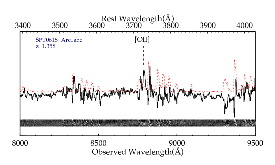
System 1 has a redshift of , determined by [OII] emission in image 1.1 (Figure 4, top panel). The galaxy has a distinctive shape, with four obvious knots. We use these knots as individual constraints. All the images in this system are secure, as are each of the knots.
System 2 consists of one long fold arc with mirror symmetry, with two secure detections. Image 2.1 has a BPZ photometric redshift , with range . A single segment for image 2.2 could not be identified; however the different segments that comprise it has a maximum redshift of 2.7. While the photometric redshifts of the two images in system 2 are disparate, the 95% confidence interval on each is consistent and broad.
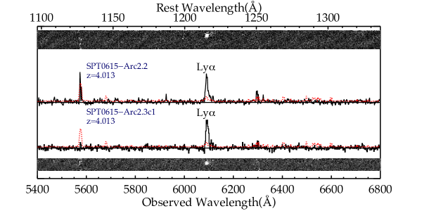
System 3 is a compact galaxy at , determined with Ly- emission (Figure 4, bottom panel). It is brightest in F814W, with a blue near-IR slope. Slits were placed on both image 3.1 and image 3.2. A redshift was measured from each slit placement. Those, along with image 3.5, are secure identifications. System 3 also has three other arc candidates that are less secure. We explore the effect of adding those images to the model in more detail below. We leave spectroscopically determined redshifts fixed during the modeling process.
In addition to the constraints discussed above, there is a candidate lensed galaxy in the field (Salmon et al., 2018). This candidate was not used as a constraint due to a lack of counter-images. See §4.2 for more details on this galaxy.
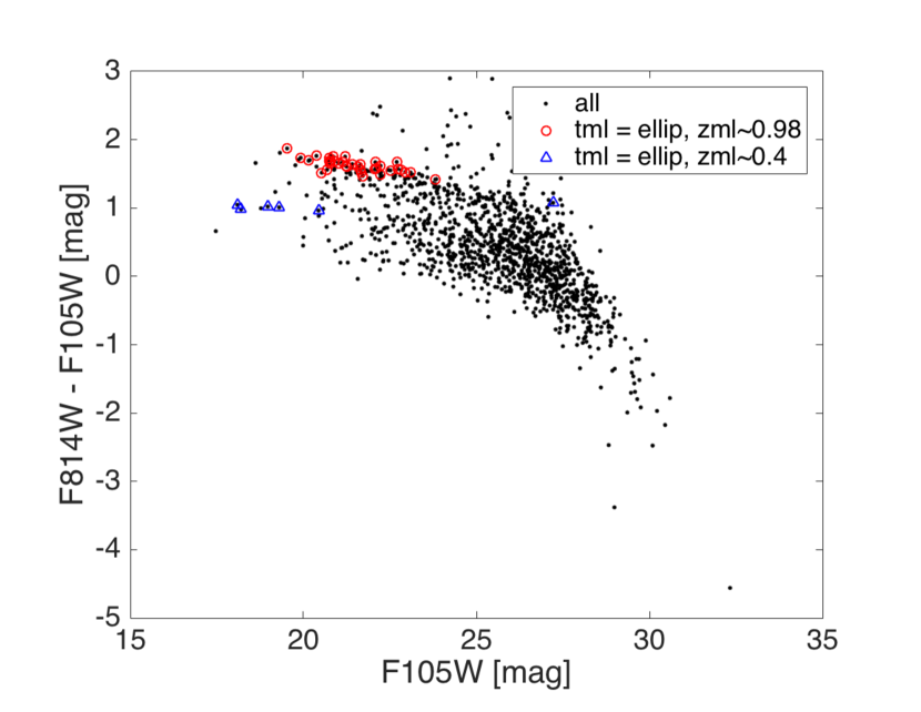
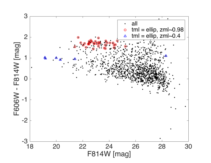
Figure 1 shows that there appears to be a foreground structure, with galaxies appearing bluer in color when compared with the color-selected galaxies of SPT0615. In Figure 3, we show the color-magnitude diagrams (CMDs) highlighting these two structures. The main cluster forms an obvious red sequence, and there appears to be a second putative red sequence for a foreground structure at , determined from the photometric redshifts of the members on the putative red sequence.
Creating the model is an iterative process. We start with one cluster-sized halo and an initial set of constraints, and add more halos and constraints until the model rms no longer improves. While photometric redshifts exist for all of the lensed systems, we leave the redshifts of systems without a spectroscopically determined redshift free to vary during the modeling process so that it will not be affected by catastrophic outliers. In SPT0615, the only system without a spectroscopically determined redshift is system 2.
Below we describe the four models that we consider, which take into account the various scenarios that can be applied to SPT0615. As mentioned above, System 3 has three secure detections, along with three other multiple image candidates that were predicted by one of the models. We create two different models, one with only the secure detections of system 3 and one with all of the detections of system 3, in order to compare them. We also note that there is foreground structure, which is described above. Because of this, we explore additional models that include the presence of a second cluster-sized halo at the redshift of SPT0615. To determine the goodness-of-fit of each model, we employ two different statistical tests. First, we compute the Bayesian Information Criterion (BIC, Schwarz, 1978):
| (1) |
where is the maximum likelihood, is the number of free parameters, and is the number of constraints.
The second test we consider is the corrected Aikake Information Criterion (AICc, Hurvich & Tsai, 1990; Cavanaugh, 1997), which helps address the potential for overfitting:
| (2) |
All terms are the same as in the BIC.
Both of these tests are used to evaluate the quality of the available models, and to assess the trade-off between the goodness-of-fit of the model and the complexity of the model. The model with the lowest BIC is preferred. To determine which model is the best using the AICc, the AICc values of each model are compared to the model with the lowest AICc value using the relative likelihood, . This is the likelihood that the model minimizes information loss when compared to the model with the lowest AICc.
The results of the statistical tests for each model are displayed in Table 3. The rms of each multiple image system in each model is displayed in Table 2.
3.1 Model 1: One Lens Plane
We first consider a model that includes all the images from systems 1 and 2, and three images from system 3. This model has one cluster-sized halo and contributions from cluster-member galaxies as described above. We fix the cut radius of this halo to 1500 kpc but allow all other parameters to vary. Because of the proximity of the images in system 1 to the central cluster galaxies, we allow the velocity dispersion of three of the central cluster galaxies to vary (shown in Figure 5) but fix all other parameters to those determined by scaling relations. This is the model with the minimum BIC, -48.00, indicating that it is the best model by the standards of that criterion (see Table 3). Compared to the other models, , meaning that the evidence in favor of this model is very strong. It is also the best model using the AICc; none of the others are likely when compared to Model 1. The critical curves for this model are shown . The model parameter results are shown in Table 4.
| Model | BIC | AICc | ||||
|---|---|---|---|---|---|---|
| 1 | 32 | 11 | 43.06 | 48.00 | 50.92 | 11.73/15 |
| 2 | 38 | 11 | 7.19 | 25.63 | 17.77 | 96.17/21 |
| 3 | 32 | 17 | 46.35 | 33.78 | 14.99 | 8.61/9 |
| 4 | 38 | 17 | 49.37 | 36.90 | 34.14 | 6.59/15 |
3.2 Model 2: One Lens Plane, All of System 3
Model 1 predicts three additional arc candidates in system 3. Candidate 3.3 is predicted to be magnitude fainter than arcs 3.1 and 3.2, but magnitudes brighter than 3.5. Candidate 3.4 is predicted to be 1.75 magnitudes brighter than arc 3.5. Arc 3.1 has and Arc 3.2 has . Arc 3.5 could not be deblended from the neighboring source and thus we were unable to measure its magnitude. Candidate 3.3 has . There are no predictions for the brightness of candidate 3.4 relative to arcs 3.1 and 3.2; however we measure its magnitude to be . Candidate 3.6 is predicted to be magnitudes fainter than arc 3.1 and magnitudes fainter than arc 3.2. It is predicted to be 2.2 magnitudes brighter than arc 3.5. We measure candidate 3.6 to be . We searched the regions of these predictions and found objects that were similar in color and morphology to the images with secure detections. Model 2 includes all six of these images, but is otherwise the same as Model 1. Table 3 shows the results of the statistical tests. Using both the BIC and AICc, this model is considered the worst or those tested. The value for this model is also higher than the value for any of the other models, and as such we do not consider it further, even taking into account the increased complexity of the model as compared to model 1. As shown below, these constraints only make sense with a second halo to account for the foreground structure.
3.3 Model 3: Foreground Structure
In this model we attempt to account for the line-of-sight structure by adding a second cluster-sized halo to the single effective lens plane. This line-of-sight structure is not associated with SPT0615, so this is not a full multiplane analysis but rather an approximation. Distance is degenerate with normalization, and with so few constraints it is difficult to disentangle the two. This approximation ignores the higher order effects discussed in McCully et al. (2014), but does approximate the amplitude and direction of the shear that a second cluster-sized halo induces. We fix the cut radius of this halo at 1800 kpc and allow all other parameters to vary. The model puts this new halo directly to the south of the first cluster-sized halo. The value for this model is comparable to that of . It is the third most likely model of the four described here.
3.4 Model 4: Foreground Structure, All of System 3
This model is the same as model 2 but adds an additional cluster-sized halo to account for the foreground structure. As with model 3, we fix the cut radius of this second cluster-sized halo at 1800 kpc and allow all other parameters to vary. If these three additional images are indeed part of system 3, as is indicated by their color and morphology, the separation is larger than expected in a typical lensing configuration, which could be caused by the presence of the foreground structure. This is the second most probable model; however, using the relative likelihood estimator described above, it is only 0.02% as likely as model 1 to be the best model. The parameters of this model are shown in Table 4.
| Object | RA | DEC | |||||
|---|---|---|---|---|---|---|---|
| (kpc) | (kpc) | (∘) | (′′) | (′′) | (km s-1) | ||
| Model 1 | |||||||
| Halo 1 | [1500] | ||||||
| Halo 2 | [0.00] | [0.00] | [0.13] | [-89.0] | [45.89] | ||
| Halo 3 | [0.21] | [1.98] | [0.43] | [-23.7] | [0.16] | [41.60] | |
| Halo 4 | [0.86] | [2.87] | [0.01] | [24.3] | [0.07] | [19.13] | |
| Model 4 | |||||||
| Halo 1 | [1500] | ||||||
| Halo 2 | [0.00] | [0.00] | [0.13] | [-89.0] | [45.89] | ||
| Halo 3 | [0.21] | [1.98] | [0.43] | [-23.7] | [0.16] | [41.60] | |
| Halo 4 | [0.86] | [2.87] | [0.01] | [24.3] | [0.07] | [10.13] | |
| Halo 5 | [1800] | ||||||
Note. — Values in brackets were held fixed during fitting. Halos 2, 3, and 4 are galaxy scale. They are labeled in cyan in Figure 5. Halo 5 takes into account the foreground structure, although it is projected to the same redshift as SPT0615, and thus the velocity dispersion is not indicative of its mass. RA and DEC are measured in the image plane. The ellipticity, , is that of the mass distribution, while is the position angle of the potential, measured counter-clockwise from horizontal.
4 Discussion and Conclusion
Based on statistical tests, Model 1 is considered the best-fitting model. We show the critical curves for this model for two different redshifts in Figure 6. The analysis that follows is based solely on Model 1. It is also the model that is available through MAST.
4.1 Strong Lensing Mass
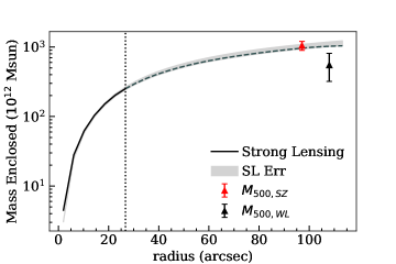
We calculate the projected mass of the cluster using the mass map generated by Lenstool (Figure 7, left). To calculate the error bars, we generate 100 maps from parameter sets sampled from the MCMC analysis and calculate the standard deviation of the distribution of calculated masses. Strong lensing mass calculations are most accurate in the region where there are constraints. Our convention is as follows: we use for the 2D projected radius and for the 3D spherical radius. For SPT0615, there are constraints out to . We find the total projected mass density within to be M☉. We also extrapolate a mass measurement to (the dashed black line in Figure 7, right) so that we may compare to other studies of this cluster. In particular, we compare our constraints to the weak lensing analysis conducted by Schrabback et al. (2018a), which is based on the mosaic ACS observations of the cluster. When centering their weak lensing measurements onto the Chandra X-ray centroid and correcting for the corresponding miscentring and mass modelling bias, these authors constrain the cluster mass to . Assuming the Diemer & Kravtsov (2015) concentration–mass relation their best-fitting mass corresponds to a spherical overdensity radius of . This WL mass constraint agrees within with the SZ constraint , which Bleem et al. (2015) obtain when assuming a mass-observable scaling relation for which the SPT cluster counts fit a CDM cosmology best (Reichardt et al., 2013). We compare these estimates of the spherical overdensity mass, plotted at the WL-estimated , to the enclosed mass from our extrapolated SL model in the right panel of Figure 7. Noting that the enclosed mass at is generally higher than a spherical overdensity mass at given the projection, we conclude that the different mass measurements are broadly consistent. Again, we emphasize that we are unable to constrain the mass slope with strong lensing this far outside the region of the strong lensing constraints. The statistical errors grossly underestimate the true uncertainties at these projected radii, and thus these estimates should be used with caution.
At M☉, SPT0615 is one of the most massive high-redshift clusters known. The only other cluster in the RELICS sample with is ACT-CLJ010249151 (“‘El Gordo”). It is at and has M☉ (Menanteau et al., 2012). A strong lensing analysis by Zitrin et al. (2013) found a lower limit of M☉, in good agreement with the SZ mass. The strong lensing analysis by Cerny et al. (2017) finds that M☉, also in good agreement. Other strong lensing clusters with complete models in this high-redshift regime include RCS 0224-0002 (, Gladders et al., 2002; Smit et al., 2017) with M☉ (Rzepecki et al., 2007), and RCS2 J232727.6-020437 (, Gilbank et al., 2011; Hoag et al., 2015; Menanteau et al., 2013) with (Sharon et al., 2015; Schrabback et al., 2018b). High-redshift clusters that show evidence of strong lensing but do not have complete models include RCS 2319530038.0 (, Gladders et al., 2002) and IDCS J1426.5+3508 (, Gonzalez et al., 2012). RCS 2319530038.0 is part of a supercluster, along with two other cluster components (Gilbank et al., 2008). It has an X-ray mass of M☉ (Hicks et al., 2008; Gilbank et al., 2008) and a weak-lensing mass of M☉ (Jee et al., 2011). The cluster IDCS J1426.5+3508 is the most massive cluster known at . Gonzalez et al. (2012) use the presence of a giant strong lensing arc to calculate the cluster mass enclosed within the arc. Extrapolating, they find M☉. Comparing SPT0615 to the other known strong-lensing clusters at high redshift, we conclude that it is not a mass outlier in the group of known strong-lensing clusters.
The high mass of SPT0615 is likely a contributing factor to its success as a lensing cluster, as it has the second highest number of high-redshift () galaxy candidates in the RELICS sample. El Gordo also has a significant number of high-redshift candidates, coming in fourth in the RELICS sample (Salmon et al., 2017). While a systematic search for high-redshift galaxy candidates has not been undertaken for the other clusters mentioned in this section, it is likely that the combination of the their high mass and high-redshift combine to make them good candidates for searching for high redshift galaxy candidates in their fields.
4.2 The Presence of a Arc
SPT0615-JD is a candidate () galaxy gravitationally lensed into an arc spanning in the field of SPT0615. It was found as part of a systematic search for high-redshift galaxies in the RELICS fields (Salmon et al., 2018). It is not visible in bands blueward of F140W.
The left panel of Figure 8 shows the location of this galaxy, along with the predicted locations of counterimages. The right panel shows the magnification map produced by our lens model for . The counter-image in the upper-right hand corner is predicted to be magnitude fainter than the original arc, placing it below the detection level of HST. Its location next to a large star also makes it difficult to search for.
Using our best-fit model, the counter-image in the east is predicted to be 0.04 magnitudes fainter than SPT0615-JD, which should be visible at the depth of our images; however a search in that region has not yielded a counter-image. The arc is aligned with the direction of the shear. We note that all the models predict counterimages in the same location and with approximately the same , with the exception of Model 3, which only predicts one counterimage to the northwest. A GLAFIC model (Oguri, 2010, Kikuchihara et al., in preparation) and Light Traces Mass (Zitrin et al., 2015) model both predict counterimages in the same location (see Salmon et al. (2018) for more details). The right panel of Figure 8 shows that SPT0615-JD is magnified by the intrinsic brightness, while the predicted counter-image would be magnified by the intrinsic brightness of the galaxy.
4.3 Conclusion
We present a strong lens model for the cluster SPT-CLJ06155746 (also known as PLCKG266.627.3) based on the presence of three multiply imaged background galaxies. Two of these multiply imaged families have confirmed spectroscopic redshifts from our observations with Magellan. The best model using the statistical results from the BIC and AICc is Model 1, which optimizes one cluster-sized dark matter halo and three smaller galaxy-sized haloes, in addition to cluster-member galaxies whose mass is determined from their light through scaling relations. This model only includes the secure observations of system 3, as well as the secure images from families 1 and 2. There are additional predicted images of system 3; however these need spectroscopic confirmation before including them in the model.
The lens model is complicated by the presence of a foreground structure, estimated to be at a photometric redshift . This is not surprising, given the prevalence of line-of-sight structure . We made versions of the lens model including this foreground structure, but the statistical analysis did not favor either version. Our analysis was not a full multiplane analysis, however, which is currently not fully supported by Lenstool. Such analysis would also benefit from spectroscopic confirmation of both the foreground candidates and multiply-imaged background galaxies.
SPT0615 is a massive high-redshift cluster, with a strong-lensing mass of M☉. Our strong lensing mass is comparable to the SZ determined mass. It is similar in mass to other strong lensing clusters in the regime, and has been shown to have magnified a high number of high-redshift background galaxies into our detection limit (Salmon et al., 2017). The field also contains a high-redshift galaxy candidate with a photometric redshift (Salmon et al., 2018).
SPT0615 is included in the RELICS program, and as such the data for this lens model are available through MAST. This data includes reduced images, catalogs, and lens models.
References
- Acebron et al. (2018) Acebron, A., Cibirka, N., Zitrin, A., et al. 2018, ApJ, 858, 42
- Anderson & Bedin (2010) Anderson, J., & Bedin, L. R. 2010, PASP, 122, 1035
- Bartelmann et al. (1998) Bartelmann, M., Huss, A., Colberg, J. M., Jenkins, A., & Pearce, F. R. 1998, A&A, 330, 1
- Bayliss et al. (2011) Bayliss, M. B., Gladders, M. D., Oguri, M., et al. 2011, ApJ, 727, L26
- Bayliss et al. (2014) Bayliss, M. B., Johnson, T., Gladders, M. D., Sharon, K., & Oguri, M. 2014, ApJ, 783, 41
- Benítez (2000) Benítez, N. 2000, ApJ, 536, 571
- Bertin & Arnouts (1996) Bertin, E., & Arnouts, S. 1996, A&AS, 117, 393
- Bleem et al. (2015) Bleem, L. E., Stalder, B., de Haan, T., et al. 2015, ApJS, 216, 27
- Cavanaugh (1997) Cavanaugh, J. E. 1997, Statistics & Probability Letters, 33, 201
- Cerny et al. (2017) Cerny, C., Sharon, K., Andrade-Santos, F., et al. 2017, ArXiv e-prints
- Chirivì et al. (2017) Chirivì, G., Suyu, S. H., Grillo, C., et al. 2017, ArXiv e-prints
- Cibirka et al. (2018) Cibirka, N., Acebron, A., Zitrin, A., et al. 2018, ArXiv e-prints
- Dalal et al. (2004) Dalal, N., Holder, G., & Hennawi, J. F. 2004, ApJ, 609, 50
- D’Aloisio & Natarajan (2011) D’Aloisio, A., & Natarajan, P. 2011, MNRAS, 411, 1628
- Diemer & Kravtsov (2015) Diemer, B., & Kravtsov, A. V. 2015, ApJ, 799, 108
- Gilbank et al. (2011) Gilbank, D. G., Gladders, M. D., Yee, H. K. C., & Hsieh, B. C. 2011, AJ, 141, 94
- Gilbank et al. (2008) Gilbank, D. G., Yee, H. K. C., Ellingson, E., et al. 2008, ApJ, 677, L89
- Gladders & Yee (2000) Gladders, M. D., & Yee, H. K. C. 2000, AJ, 120, 2148
- Gladders et al. (2002) Gladders, M. D., Yee, H. K. C., & Ellingson, E. 2002, AJ, 123, 1
- Gonzaga & et al. (2012) Gonzaga, S., & et al. 2012, The DrizzlePac Handbook
- Gonzalez et al. (2012) Gonzalez, A. H., Stanford, S. A., Brodwin, M., et al. 2012, ApJ, 753, 163
- Hennawi et al. (2007) Hennawi, J. F., Dalal, N., Bode, P., & Ostriker, J. P. 2007, ApJ, 654, 714
- Hicks et al. (2008) Hicks, A. K., Ellingson, E., Bautz, M., et al. 2008, ApJ, 680, 1022
- Ho & White (2005) Ho, S., & White, M. 2005, Astroparticle Physics, 24, 257
- Hoag et al. (2015) Hoag, A., Bradač, M., Huang, K. H., et al. 2015, ApJ, 813, 37
- Horesh et al. (2011) Horesh, A., Maoz, D., Hilbert, S., & Bartelmann, M. 2011, MNRAS, 418, 54
- Huang et al. (2009) Huang, X., Morokuma, T., Fakhouri, H. K., et al. 2009, ApJ, 707, L12
- Hurvich & Tsai (1990) Hurvich, C. M., & Tsai, C.-L. 1990, Statistics & Probability Letters, 9, 259
- Jaroszynski & Kostrzewa-Rutkowska (2014) Jaroszynski, M., & Kostrzewa-Rutkowska, Z. 2014, MNRAS, 439, 2432
- Jee et al. (2011) Jee, M. J., Dawson, K. S., Hoekstra, H., et al. 2011, ApJ, 737, 59
- Johnson & Sharon (2016) Johnson, T. L., & Sharon, K. 2016, ApJ, 832, 82
- Jullo et al. (2007) Jullo, E., Kneib, J.-P., Limousin, M., et al. 2007, New Journal of Physics, 9, 447
- Li et al. (2005) Li, G.-L., Mao, S., Jing, Y. P., et al. 2005, ApJ, 635, 795
- Limousin et al. (2005) Limousin, M., Kneib, J.-P., & Natarajan, P. 2005, MNRAS, 356, 309
- McCully et al. (2014) McCully, C., Keeton, C. R., Wong, K. C., & Zabludoff, A. I. 2014, MNRAS, 443, 3631
- McCully et al. (2017) —. 2017, ApJ, 836, 141
- Menanteau et al. (2012) Menanteau, F., Hughes, J. P., Sifón, C., et al. 2012, ApJ, 748, 7
- Menanteau et al. (2013) Menanteau, F., Sifón, C., Barrientos, L. F., et al. 2013, ApJ, 765, 67
- Meneghetti et al. (2017) Meneghetti, M., Natarajan, P., Coe, D., et al. 2017, MNRAS, 472, 3177
- Oguri (2010) Oguri, M. 2010, PASJ, 62, 1017
- Paterno-Mahler et al. (2017) Paterno-Mahler, R., Blanton, E. L., Brodwin, M., et al. 2017, ApJ, 844, 78
- Planck Collaboration et al. (2011) Planck Collaboration, Ade, P. A. R., Aghanim, N., et al. 2011, A&A, 536, A8
- Planck Collaboration et al. (2016) —. 2016, A&A, 594, A27
- Reichardt et al. (2013) Reichardt, C. L., Stalder, B., Bleem, L. E., et al. 2013, ApJ, 763, 127
- Rzepecki et al. (2007) Rzepecki, J., Lombardi, M., Rosati, P., Bignamini, A., & Tozzi, P. 2007, A&A, 471, 743
- Salmon et al. (2017) Salmon, B., Coe, D., Bradley, L., et al. 2017, ArXiv e-prints
- Salmon et al. (2018) —. 2018, ArXiv e-prints
- Sand et al. (2005) Sand, D. J., Treu, T., Ellis, R. S., & Smith, G. P. 2005, ApJ, 627, 32
- Schrabback et al. (2018a) Schrabback, T., Applegate, D., Dietrich, J. P., et al. 2018a, MNRAS, 474, 2635
- Schrabback et al. (2018b) Schrabback, T., Schirmer, M., van der Burg, R. F. J., et al. 2018b, A&A, 610, A85
- Schwarz (1978) Schwarz, G. 1978, Annals of Statistics, 6, 461
- Sharon et al. (2015) Sharon, K., Gladders, M. D., Marrone, D. P., et al. 2015, ApJ, 814, 21
- Smit et al. (2017) Smit, R., Swinbank, A. M., Massey, R., et al. 2017, MNRAS, 467, 3306
- Wambsganss et al. (2004) Wambsganss, J., Bode, P., & Ostriker, J. P. 2004, ApJ, 606, L93
- Williamson et al. (2011) Williamson, R., Benson, B. A., High, F. W., et al. 2011, ApJ, 738, 139
- Wright et al. (2010) Wright, E. L., Eisenhardt, P. R. M., Mainzer, A. K., et al. 2010, AJ, 140, 1868
- Wylezalek et al. (2014) Wylezalek, D., Vernet, J., De Breuck, C., et al. 2014, ApJ, 786, 17
- Xu et al. (2016) Xu, B., Postman, M., Meneghetti, M., et al. 2016, ApJ, 817, 85
- Zitrin et al. (2013) Zitrin, A., Menanteau, F., Hughes, J. P., et al. 2013, ApJ, 770, L15
- Zitrin et al. (2015) Zitrin, A., Fabris, A., Merten, J., et al. 2015, ApJ, 801, 44