Introduction to the Dicke model: from equilibrium to nonequilibrium, and vice versa

Abstract

The Dicke model describes the coupling between a quantized cavity field and a large ensemble of two-level atoms. When the number of atoms tends to infinity, this model can undergo a transition to a superradiant phase, belonging to the mean-field Ising universality class. The superradiant transition was first predicted for atoms in thermal equilibrium and was recently realized with a quantum simulator made of atoms in an optical cavity, subject to both dissipation and driving. In this Progress Report, we offer an introduction to some theoretical concepts relevant to the Dicke model, reviewing the critical properties of the superradiant phase transition, and the distinction between equilibrium and nonequilibrium conditions. In addition, we explain the fundamental difference between the superradiant phase transition and the more common lasing transition. Our report mostly focuses on the steady states of atoms in single-mode optical cavities, but we also mention some aspects of real-time dynamics, as well as other quantum simulators, including superconducting qubits, trapped ions, and using spin-orbit coupling for cold atoms. These realizations differ in regard to whether they describe equilibrium or non-equilibrium systems.

I Historical background

Superradiance was first introduced in 1954 by Dicke to describe the emission of light by a large ensemble of atoms^{Dicke (1954)}. Dicke considered $N$ two-level atoms that are initially prepared in their excited state. At a given time, one of the atoms decays by emitting a photon. This induces a chain reaction that leads to the decay of all the $N$ atoms and the emission of $N$ photons in free space. Dicke explained that if all the atoms are trapped within a fraction of a wavelength, the photons emitted will be indistinguishable. In this case, the emission processes will interfere constructively, giving rise to an electromagnetic field with amplitude proportional to $N$ and an energy density proportional to $N^{2}$. The scaling laws of this transient superradiance differ from the decay of $N$ independent atoms, where the light is emitted incoherently and has an energy density proportional to $N$.

In 1973, Hepp and Lieb^{Hepp and Lieb (1973)} discovered a different type of steady-state superradiance, which occurs when the ensemble of atoms is coupled to the quantized mode of a cavity. They considered the thermal equilibrium properties of the resulting Dicke model and demonstrated that it shows a continuous phase transition between a normal and a superradiant phase. To achieve a meaningful thermodynamic limit, Hepp and Lieb^{Hepp and Lieb (1973)} assumed that the coupling between the two level systems and the photon field decreases as $1/\sqrt{N}$. Under this assumption, in the normal phase, the number of photons $n$ does not grow with $N$, while in the superradiant phase, $n$ is proportional to $N$. The paper by Hepp and Lieb is written in a mathematical style, which was soon reformulated in a form more transparent to physicists by Wang and Hioe^{Wang and Hioe (1973)}. Their analysis was later refined by Refs. Hioe (1973); Carmichael et al. (1973); Duncan (1974) who showed that the transition survives in the presence of counter-rotating terms, which however shift the position of the transition by a factor of 1/2.

In spite of the significant theoretical interest, the superradiant transition had not been realized experimentally, until recent times. The major difficulty is that the transition requires very strong coupling between the atoms and the cavity, such that the photon-atom coupling is of the order of the atomic and cavity frequencies. From a theoretical perspective, several authors studied whether the superradiant transition can be reached using only the dipole coupling between the atoms and the cavity. These studies gave rise to a fundamental debate around the validity of a no-go theorem for the superradiant transition, which will be discussed in Sec. II.4.

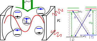
Figure 1: Schematic representation of the driven-dissipative Dicke model, based on internal degrees of freedom and proposed by Dimer et al.^{Dimer et al. (2007)}. In this realization, each atom is modeled by a 4-level scheme and is coupled to the cavity through stimulated Raman emissions. In the steady state, the system absorbs energy from the external time dependent pump (at frequency $\omega_{p}$) and dumps it into several dissipative channels ($\gamma_{\downarrow}$ and $\kappa$).

In the last decade, two uncontested ways to realize the Dicke model and its superradiant transition have been demonstrated theoretically and experimentally. The first approach was proposed by Dimer et al.^{Dimer et al. (2007)} and is based on a 4-level scheme (see Fig. 1). In this setup, the coupling between the atoms and the photons is induced by stimulated Raman emission, and can be made arbitrarily strong. This proposal was recently realized by Zhiqiang et al..^{Zhiqiang et al. (2017)}. The second approach was inspired by an earlier experiment, proposed by Domokos and Ritsch^{Domokos and Ritsch (2002)}, and realized by Black et al.^{Black et al. (2003)}. These authors considered a gas of thermal atoms that are trapped inside a cavity. The atoms are illuminated by an external coherent pump and scatter photons into the cavity (see Fig. 2). It was found that for strong enough pump intensities, the atoms self-organize in a checkerboard pattern, where the atoms are preferentially separated by an integer multiple of the photon’s wavelength, and scatter light coherently. This analysis was later extended to the case of a Bose-Einstein condensate (BEC) theoretically by Nagy et al.^{Nagy et al. (2010)} and experimentally by Baumann et al.^{Baumann et al. (2010)}. In a BEC, the atoms are delocalized, and the phase of the scattered light is random. In this situation, the scattered photons are incoherent and their number does not grow with $N$. In contrast, in the self-organized state, all atoms emit photons coherently, giving rise to a superradiant phase, where the number of photons is proportional to $N$. Following this reasoning, Refs. Nagy et al. (2010); Baumann et al. (2010) showed that the onset of self-organization can be mapped to the superradiance transition of the Dicke model, see Sec. II. This study was later extended to narrow linewidth^{Klinder et al. (2015)} and multimode^{Vaidya et al. (2018)} cavities.

The two above-mentioned realizations of the superradiant transition in the Dicke model involve driven-dissipative systems. In both settings, the coupling between the atoms and the photons is achieved through an external time-dependent pump. This allows arbitrarily strong effective light-matter coupling strengths, enabling the transition. As a consequence of being driven, these systems cannot be described by an equilibrium Dicke model, but one needs to take into account the drive and dissipation present. This subtle difference was initially dismissed because, in the limit of vanishing losses, the critical coupling of the driven-dissipative model coincides with the value of the equilibrium case, see Sec. III. Because the driven-dissipative model does not have a well-defined temperature, it was tempting to identify the experiment with a zero-temperature quantum phase transition. However, later studies^{Nagy et al. (2011); Öztop et al. (2012); Dalla Torre et al. (2013)} showed that the phase transition has the same universal properties as the equilibrium transition at finite temperature. This equivalence can be understood in terms of an emergent low-frequency thermalization, which will be reviewed in Sec. IV. These approaches can be considered as analog quantum simulators of the Dicke model: the driving scheme is designed to engineer an effective Dicke model with tunable parameters allowing exploration of the phase diagram. As discussed further in Sec. II.4, there also exist proposals for digital or hybrid analog-digital quantum simulation of the Dicke model using superconducting qubits or trapped ions^{Mezzacapo et al. (2014); Lamata (2017); Aedo and Lamata (2018)}.

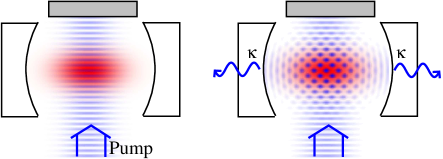
Figure 2: Cartoon of the self-organization transition. When the pump strength is below threshold (left), the atoms are delocalized and scatter light incoherently in the cavity. Above threshold (right) the atoms feel an optical lattice from the interference of pump and cavity light, and organize into a checkerboard lattice. Adapted from Ref. Keeling et al. (2010).

The main goals of this Progress Report are (i) to present simple physical arguments to understand the commonalities and differences between the superradiant phase transition in the equilibrium Dicke model and its non-equilibrium counterparts (Secs. II-IV), (ii) to introduce some analytical and numerical approximations, used to study the Dicke model (Sec. V); and (iii) to set the superradiant transition in the wider context of closely related models and transitions (Sections VI and VII). For a broader discussion of the phenomena of superradiance and the Dicke model, we refer the reader to a number of other relevant reviews: Gross and Haroche^{Gross and Haroche (1982)} discusses the transient superradiance first predicted by Dicke; Garraway^{Garraway (2011)} presents the Dicke model and its phase transitions from a quantum optics perspective; Ritsch et al.^{Ritsch et al. (2013)} discusses the self organization of atoms in optical cavities and dynamical optical lattices.

II Models and experiments

II.1 The Dicke model at equilibrium

The Dicke model describes a single bosonic mode (often a cavity photon mode) which interacts collectively with a set of $N$ two-level systems (the atoms). The Dicke Hamiltonian is given by

$$H=\omega_{c}a^{\dagger}a+\omega_{z}\sum_{j=1}^{N}\sigma^{z}_{j}+\frac{2\lambda}{\sqrt{N}}(a+a^{\dagger})\sum_{j}\sigma^{x}_{j}\;.$$ (1)

Here $a^{\dagger}(a)$ are the creation (annihilation) operators of the photon, satisfying $[a,a^{\dagger}]=1$, and $\sigma^{\alpha}_{i}$ are spin operators, satisfying $[\sigma^{x}_{j},\sigma^{y}_{k}]=i\delta_{j,k}\sigma^{z}_{j}$ (note that $\sigma^{\alpha}=\tau^{\alpha}/2$, where $\tau^{\alpha}$ are Pauli matrices). The model has three tuning parameters: the photon frequency $\omega_{c}$, the atomic energy splitting $\omega_{z}$, and the photon-atom coupling $\lambda$.

To understand the nature of the superradiant transition, it is useful to analyze the symmetries of this model. By applying the transformation $a\to-a$ and $\sigma^{x}\to-\sigma^{x}$, the Hamiltonian remains unchanged. This gives a symmetry group with only two elements (when this transformation is applied twice it brings back to the original state) and is formally associated with a $\mathbb{Z}_{2}$ group. This symmetry arises due to the conservation of the parity of the total number of excitations (i.e. the number of photons, plus the number of excited spins), and is analogous to the Ising symmetry of ferromagnets. As we will see, the superradiant transition indeed shares the same critical exponents as the mean-field Ising transition.

The Dicke model, Eq. (1), depends on the atomic degrees of freedom through the total spin operators $S^{\alpha}=\sum_{j}\sigma^{\alpha}_{j}$ only. Using this definition, the Dicke model becomes

$$H=\omega_{c}a^{\dagger}a+\omega_{z}S^{z}+\frac{2\lambda}{\sqrt{N}}(a+a^{\dagger})S^{x}\,.$$ (2)

This Hamiltonian commutes with the total spin $S^{2}=(S^{x})^{2}+(S^{y})^{2}+(S^{z})^{2}$. Consequently, it connects only states with the same total spin $S$, i.e. that belong to the same Dicke manifold. This symmetry provides a significant simplification of the problem because it allows the description of the atomic degrees of freedom in terms of $N+1$ states, rather than the entire Hilbert space of size $2^{N}$^{Chen et al. (2008)}. This symmetry can however be broken by physical processes that act on individual atoms, which will be described in Sec. II.3.

II.2 Raman transitions and self-organization

As mentioned in the introduction, the Dicke model was realized experimentally in two ways: (i) using stimulated Raman emission between two hyperfine states in the ground state manifold of a cold atomic cloud, and (ii) coupling to the motional degrees of freedom of a BEC.

The former realization^{Dimer et al. (2007)} involves a 4-level scheme, schematically drawn in Fig. 1. The mapping to the Dicke model is straightforward: $\omega_{z}$ is the effective splitting between the two ground states (taking into account any differential Stark shifts due to the external drive), and $\lambda/\sqrt{N}$ the strength of the stimulated Raman emission into the cavity mode. Note that this coupling is achieved by using two distinct external fields. These two processes correspond to $\sigma^{+}_{i}a+\sigma^{-}_{i}a^{\dagger}$ and $\sigma^{+}_{i}a^{\dagger}+\sigma^{-}_{i}a^{\dagger}$, respectively, and are often referred to as rotating and counter-rotating. When the two processes have equal strength, one recovers the Dicke model of Eq. (1). By varying the relative strength, it is possible to realize a generalized Dicke model, with different prefactors to the rotating and counter-rotating terms, which will be discussed further in Sec. VI.2.

In the latter realization^{Nagy et al. (2010); Baumann et al. (2010)}, the mapping to the Dicke model was achieved by considering two momentum modes of the atoms (the BEC at $q=0$ and the first recoil at $k_{L}=2\pi/\lambda$). It is not immediately clear that this mapping is completely justified. Firstly, it is not a priori clear that one may neglect higher order scatterings, at multiples of $k_{L}$. Secondly, the mapping only holds if the atoms are initially found in a BEC. However, in practice, the self-organization transition occurs in a thermal state as well^{Domokos and Ritsch (2002); Black et al. (2003)}: a detailed analysis revealed that the superradiance phase transition is essentially unaffected by the BEC transition^{Piazza et al. (2013)}.

Hence, we present here a different mapping of the self-organization transition to the Dicke model, which does not require a BEC. Our derivation assumes that the atoms do not interact and are initially found in the superradiant phase. In this state, the atoms scatter light into a standing wave of the cavity field, whose period is $\lambda/2$. However, to enable superradiance, the atoms need to preferentially occupy sites that are separated by an integer multiple of $\lambda$ in the longitudinal direction of the cavity. Having denoted all the possible sites as even or odd, we introduce the spin variables $\sigma^{x}_{j}$, which indicate whether the atom $j$ is on an even ($\sigma^{x}_{j}=1/2$) or odd ($\sigma^{x}_{j}=-1/2$) site. Depending on their positions, the atoms scatter light from the pump, and create cavity photons, with a phase of either $0$ or $\pi$. If we define $N_{\rm even}$ and $N_{\rm odd}$ as the operators that count the number of atoms on the even and odd sites, respectively, the photon-atom coupling can be written as $\lambda(t)a^{\dagger}(N_{\text{even}}-N_{\text{odd}})+{\rm H.c.}=2\lambda(t)a^{\dagger}\sum_{j}\sigma^{x}_{j}+{\rm H.c.}$, where $\lambda(t)=\lambda\exp(i\omega_{p}t)$ is proportional to the pump field and oscillates at the pump frequency $\omega_{p}$. In addition, the atoms can experience quantum tunneling between even and odd sites. This process is described by the spin-flip operator $\omega_{z}\sigma^{z}_{j}$, where $\omega_{z}$ is the tunnelling rate.

By combining these terms, we obtain the Dicke model

$$H(t)=\omega_{c}a^{\dagger}a+\omega_{z}\sum_{j=1}^{N}\sigma^{z}_{j}+2\left(\lambda(t)a+\lambda^{*}(t)a^{\dagger}\right)\sum_{j=1}^{N}\sigma^{x}_{j}.$$ (3)

In general, the parameters in this model may have a non-trivial dependence on the pump strength. (For instance in a standing-wave pump profile, the tunneling matrix element is given by the difference of eigenvalues of the Mathieu equation. See the Appendix A.1 of Ref. Bhaseen et al. (2012).) On approaching the transition, the standing wave becomes weaker and $\omega_{z}$ achieves its maximal possible value, which equals to the recoil energy $E_{R}=k_{L}^{2}/2m$. In this limit, Eq. (3) becomes identical to the Dicke model obtained by Ref. Nagy et al. (2010), which started by considering a BEC of atoms.

II.3 Driven-dissipative models

The explicit time dependence of Eq. (3) can be removed by shifting to an appropriate rotating frame, i.e. by using the gauge transformation $a\to e^{i\omega_{p}t}a$. This transformation brings Eq. (3) to the time-independent Dicke model, Eq. (1), with a renormalized cavity frequency $\omega_{c}\to\omega_{c}-\omega_{p}$. If the system were closed, this transformation would have no physical consequences. However, when the system is coupled to a bath, the transformation changes the properties of the bath, pushing it out of equilibrium. In particular, since all frequencies are renormalized down by $\omega_{p}$, the transformation leads to a bath with both positive and negative frequencies, while equilibrium baths have positive eigenfrequencies only. Hence, there are two equivalent ways to describe the driven-dissipative Dicke model: (i) in the laboratory frame, where the bath is in thermal equilibrium but the Hamiltonian is time dependent, and (ii) in the rotating frame, where the Hamiltonian is time independent, but the baths are effectively out of equilibrium.

In this report we follow the second, more common approach, and work in the rotating frame. Since the optical frequency is the largest scale in the problem, the baths can be approximated as Markovian^{Scully and Zubairy (1997)}. As discussed for example in Ref. Dalla Torre et al. (2013), Markovian baths generally violate the equilibrium fluctuation-dissipation relation. This is because of the negative frequency bath components described above. These cannot be found at thermal equilibrium because their partition function is not normalizable (for a bath mode at frequency $\omega_{b}<0$, $Z=Tr[e^{\beta|\omega_{b}|a^{\dagger}a}]\to\infty$). In practice, this is not a problem because the occupation of the bath modes is actually set by their frequencies in the laboratory frame $\omega_{p}+\omega_{b}>0$, rather than in the rotating frame, $\omega_{b}<0$.

For optical frequencies at room temperature, the occupation of the bath modes can be safely approximated to zero, giving rise to the Lindblad-form master equation

$$\dot{\rho}=-i[H,\rho]+\sum_{i}\gamma_{i}\mathcal{D}\left[L_{i}\right]$$ (4)

where $\rho$ is the system’s density matrix, and

$$\mathcal{D}\left[L\right]\equiv 2L\rho L^{\dagger}-\left\{L^{\dagger}L,\rho\right\}.$$ (5)

Physically, the rates $\gamma_{i}$ and operators $L_{i}$ correspond to different sources of dissipation. For experiments on the Dicke model, the most relevant sources of dissipation are listed in Table 1, and can be divided in two main categories: collective effects ($\kappa$ and $\gamma$) and single atoms effects ($\gamma_{\downarrow}$ and $\gamma_{\phi}$). In Sec. III we will explain how to deal with these categories. Other sources of dissipation, such as the loss of atoms, require going beyond the picture of a fixed number of two-level systems coupled to light, and will not be considered here.

rate	L operator	physical process
$\kappa$	$a$	cavity decay
$\gamma$	$\sum_{j}\sigma^{-}_{j}=S^{-}$	collective atomic decay
$\gamma_{\downarrow}$	$\sigma^{-}_{j}$	single-atom decay
$\gamma_{\phi}$	$\sigma^{z}_{j}$	single-atom dephasing

Table 1: Main sources of dissipation that were considered in the literature^{Dalla Torre et al. (2016); Kirton and Keeling (2017); Zhiqiang et al. (2018)} .

II.4 Other realizations of the Dicke model

In Sec. I, we mentioned a no-go theorem for the superradiant transition by Rzazewski^{Rzażewski et al. (1975)}. These authors claimed that the superradiant transition cannot be reached using dipole couplings between atoms and photons. The key observation of Rzazewski^{Rzażewski et al. (1975)} is that the Dicke model is incomplete, because it is not invariant under gauge transformations of the electromagnetic field. A minimal change which recovers this invariance is to add a term proportional to the square of the vector potential. The Thomas-Reiche-Kuhn sum rule then implies that the strength of this additional term is exactly that needed to inhibit the phase transition, leading to a “no-go” theorem^{Bialynicki-Birula and Rzażewski (1979); Keeling (2007)}.

The validity of this no-go theorem is still debated. In particular, a full quantum treatment of the problem requires not only the $A^{2}$ terms, but a description of the longitudinal Coulomb interactions between dipoles. By considering a full description of a realistic system of atoms in a real cavity, Refs. Vukics and Domokos (2012); Vukics et al. (2014, 2015); Grießer et al. (2016); De Bernardis et al. (2018a) showed that a phase transition can occur in the right geometry. Since the “photon creation” operator describes different physical fields in different gauges, it is important to check what physical fields acquire macroscopic expectations in such a transition. Such analysis reveals that this transition is adiabatically connected to a crystalline transition for motional degrees of freedom^{Vukics et al. (2015)}, or to a ferroelectric transition for dipole couplings^{De Bernardis et al. (2018a)}. Very recent works^{De Bernardis et al. (2018b); Stokes and Nazir (2018)} have also noted that since the two-level approximation has a different meaning in different gauges, its validity at strong coupling is not gauge invariant: as such^{De Bernardis et al. (2018b)} shows that only in the dipole gauge can the two-level approximation be trusted. The question of how to properly describe matter–light coupling has also recently been discussed in the context of combining cavity quantum electrodynamics with density functional theory^{Flick et al. (2017); Rokaj et al. (2018)}.

The realization of the Dicke model using Raman driving circumvents the no-go theorem, for the following reasons: Firstly, the effective matter-light couplings appearing in this Hamiltonian are a combination of the bare coupling, the pump strength and the detuning. As such, these are not subject to any oscillator-strength sum-rule. Moreover, even the bare couplings appearing in the effective coupling relate to transitions between ground and excited atomic states, rather than direct transitions between the low energy states forming the two-level system. Finally, the effective cavity frequency is tunable through the pump-cavity detuning. As a result of all of these points, there is no longer any constraint on the relation between the parameters of the model, and a superradiant transition is possible. An $A^{2}$ term may nonentheless be present, but the system’s parameters can be chosen such that this term is weak enough to be ignored.

In addition, the original equilibrium superradiant transition of the Dicke model is possible in a grand canonical ensemble^{Eastham and Littlewood (2000, 2001)}. In such an ensemble, one minimizes the grand potential $\Phi=-k_{B}T\ln(Z_{\rm GC})$, where $Z_{\rm GC}={\rm Tr}\left[\exp(-\beta(H-\mu N_{\rm ex}))\right]$, and $N_{\text{ex}}=a^{\dagger}a+\sum_{j}\sigma^{z}_{j}+1/2$. The chemical potential $\mu$ shifts the effective parameters $\omega_{c},\omega_{z}\to\omega_{c}-\mu,\omega_{z}-\mu$ such that the sum rule required for the no-go theorem no longer holds. Considering this ensemble only makes sense if the Hamiltonian preserves the number of excitations, i.e. working in the limit where counter-rotating terms can be dropped, giving rise to the Tavis–Cummings model (see Sec. VI.1). Conceptually, this corresponds to considering a perfect cavity prepared with an initial finite excitation density and then asking for the ground state. This model can also describe the Bose–Einstein condensation of exciton-polaritons — superpositions of microcavity photons and excitons^{Deng et al. (2010); Carusotto and Ciuti (2013)} — in the limit of a very good cavity^{Kasprzak et al. (2006); Sun et al. (2017)}.

Another context in which the Dicke transition is expected to be possible involves circuit QED^{Houck et al. (2012)}. Here, the two-level atoms are replaced by superconducting qubits, coupled to a common microwave resonator. This again can be considered as an analog quantum simulator, with the superconducting qubits acting as tunable artificial atoms. There has been much discussion on whether the Hamiltonian describing such a system should contain $A^{2}$ terms, and as such, whether it is subject to the no-go theorem^{Nataf and Ciuti (2010); Viehmann et al. (2011); Ciuti and Nataf (2012); Lambert et al. (2016); Bamba et al. (2016); Jaako et al. (2016); Bamba and Imoto (2017)}. For at least some designs of circuit, if one starts from the classical Kirchoff equations (i.e. conditions on the currents and voltages) of the circuit, and proceeds to quantize these equations, the resulting Hamiltonian is not necessarily subject to the no-go theorem. i.e., there are cases where either the $A^{2}$ term is absent, or where it is present, but with a weaker coupling strength than required to prevent the phase transition.

The above realizations of the Dicke model involve coupling to a photonic mode, at optical or microwave frequencies. In addition, the Dicke model can be realized in any case where many spin degrees of freedom couple to a common bosonic mode. There have been several proposals for realizing such a model where the bosonic mode corresponds to motion in an harmonic trap, i.e. a mechanical phonon mode, rather than a photon.

One widely studied example involves coupling the electronic states of trapped ions to their center of mass motion^{Genway et al. (2014); Pedernales et al. (2015); Aedo and Lamata (2018); Safavi-Naini et al. (2018)}. In fact, the natural coupling between a standing wave laser and an ion leads to a position dependent matrix element^{Leibfried et al. (2003)}. Writing this position in terms of vibrational raising and lowering operators, one can expand in the Lamb-Dicke regime to produce an effective Dicke model^{Pedernales et al. (2015); Aedo and Lamata (2018)}. Alternately, a state-dependent optical potential can be used to couple the electronic state of the ion to the center of mass mode^{Porras and Cirac (2004); Wang et al. (2013); Genway et al. (2014)}. Such an approach has been realized experimentally in Ref. Safavi-Naini et al. (2018), where an adiabatic sweep from the normal to the superradiant state has been studied.

A similar idea has also been realized by Hamner et al.^{Hamner et al. (2014)}, using a spin-orbit coupled BEC in an harmonic trap. Here spin-orbit coupling produces a coupling between atomic motion and the internal spin state. The cloud of atoms is reduced to a single motional degree of freedom by the non-fragmentation of an interacting BEC. Using this mapping to the Dicke model, the experimentally observed transition between a polarized and unpolarized state of the atoms can be understood as an analogue of the superradiant phase transition.

All the above examples describe various routes to analog quantum simulation of the Dicke model, i.e. they involve directly engineering a Dicke Hamiltonian, and then studying the steady state or dynamics of this model. In addition, there have been other proposals to use digital quantum simulation, i.e. to replace time evolution under the Dicke Hamiltonian with a sequence of discrete unitary gates that leads to the same evolution. In particular, schemes have been proposed to realize such digital quantum simulation using superconducting qubits^{Mezzacapo et al. (2014); Lamata (2017)}.

III Threshold of the superradiant transition

In this section we give an overview of some simple techniques for finding the critical point in the Dicke model both in and out of equilibrium. These approaches are based on mean-field theory, and give an intuitive understanding of the superradiant transition.

III.1 Equilibrium transition

In equilibrium we can calculate the critical coupling of the Dicke model, Eq. (1), by minimizing its mean-field free energy. Within this approach, we assume the photons to be in a coherent state $|\alpha\rangle$, defined by $a|\alpha\rangle=\alpha|\alpha\rangle$, where $\alpha$ is a real variational parameter. In this state, the energy of the cavity is $\omega_{c}{\langle a^{\dagger}a\rangle}=\omega_{c}\alpha^{2}$ and each atom experiences the Hamiltonian

$$h(\alpha)=\omega_{z}\sigma_{i}^{z}+\frac{4\lambda}{\sqrt{N}}\alpha\sigma_{i}^{x}\;.$$ (6)

The partition function is then given by

$$Z(\alpha)={\rm Tr}[e^{-\beta H}]={\rm e}^{-\beta\omega_{c}\alpha^{2}}\left(\operatorname{\mathrm{Tr}}{\rm e}^{-\beta h}\right)^{N}\;,$$ (7)

where $\beta=1/T$ is the inverse temperature. By definition, the free energy is

$$F(\alpha)=-\frac{1}{\beta}\ln(Z(\alpha))=\omega_{c}\alpha^{2}-\frac{N}{\beta}\ln\left(2\cosh{\beta E}\right)\,,$$ (8)

where $E=\sqrt{\frac{\omega_{z}^{2}}{4}+\frac{4\lambda^{2}}{N}\alpha^{2}}$ is the eigenvalue of $h(\alpha)$.

By optimizing $F$ as a function of $\alpha$, one finds that if $\lambda<\lambda_{c}$ the minimum is at $\alpha=0$ while for $\lambda>\lambda_{c}$ the minimum is at $\alpha\neq 0$. The critical value $\lambda_{c}$ is found by the condition $F^{\prime\prime}(\alpha=0)=0$, or

$$\lambda_{c}=\frac{1}{2}\sqrt{\omega_{c}\omega_{z}\coth\left(\frac{\beta\omega_{z}}{2}\right)}.$$ (9)

Note that this critical coupling smoothly evolves down to zero temperature ($\beta\to\infty$), where one obtains $\lambda_{c}=\sqrt{\omega_{c}\omega_{z}}/2$.

One may also use the above approach to find the critical exponent $\beta$ that controls how the order parameter $\alpha$ evolves beyond the critical $\lambda$. In general, for $\lambda>\lambda_{c}$ we minimize the free energy by solving $dF(\alpha)/d\alpha=0$, or

$$\omega_{c}\alpha=\frac{N}{2}\tanh(\beta E)\frac{dE}{d\alpha}=\frac{2\lambda^{2}\tanh(\beta E)}{E}\alpha,$$ (10)

and since $\alpha\neq 0$ this gives $\omega_{c}E=2\lambda^{2}\tanh(\beta E)$. For small $\alpha$ we can expand $E=(\omega_{z}/2)+4\lambda^{2}\alpha^{2}/N\omega_{z}$. Expanding both sides of Eq. (10) to order $\alpha^{2}$, one finds

$$\alpha=\sqrt{N\mathcal{A}(\lambda)(\lambda^{2}-\lambda_{c}^{2})},$$ (11)

where $\mathcal{A}(\lambda)$ is a function of coefficients which is finite at $\lambda=\lambda_{c}$ for all temperatures. One finds that in the superradiant state, the order parameter scales as $\sqrt{N}$ and develops as $\alpha\sim(\lambda-\lambda_{c})^{\beta}$, with $\beta=1/2$. These results are valid both for zero and non-zero temperatures. Nevertheless, as we will explain in Sec. IV, the these two transitions are actually fundamentally different.

III.2 Holstein–Primakoff transformation

An alternative description of the Dicke model relies on the Holstein-Primakoff (HP) representation^{Holstein and Primakoff (1940)}, which maps the total spin operators $S^{\alpha}$ to a bosonic mode $b$

$$S^{z}\to-\frac{N}{2}+b^{\dagger}b,~{}~{}~{}~{}~{}S^{+}\to b^{\dagger}\sqrt{{N}-b^{\dagger}b}\,.$$ (12)

In the large $N$ limit (where $N\gg{\langle b^{\dagger}b\rangle}$), Eq. (12) simplifies to $S^{x}\to\sqrt{N}(b+b^{\dagger})$ and the Dicke model, Eq. (2), becomes equivalent to two coupled Harmonic oscillators

$$H_{HP}=\omega_{c}a^{\dagger}a+\omega_{z}b^{\dagger}b+\lambda(a+a^{\dagger})(b+b^{\dagger})\;.$$ (13)

Since the HP transformation relies on the total spin representation, this approach can include collective decay channels only, $\kappa$ and $\gamma$ in Table 1^{Gelhausen et al. (2017)}. Being a quadratic Hamiltonian, the model (13) can be analytically solved at equilibrium, as well as out of equilibrium, in many different ways. In the following sections we will briefly summarize how this is done using master equations, as well as Keldysh path integrals.

Within the master equation approach, Eq. (4), one has

$$\dot{\rho}=-i[H_{HP},\rho]+\kappa\mathcal{D}[a]+\gamma\mathcal{D}[b].$$ (14)

Eq. (14) gives rise to linear equations of motion for the operators $a$ and $b$, which can be equivalently rewritten in terms of classical expectations,

$$\dot{a} =(-i\omega_{c}-\kappa)a-i\lambda(b+b^{\dagger})$$ (15)

$$\dot{b} =(-i\omega_{z}-\gamma)b-i\lambda(a+a^{\dagger}).$$ (16)

These equations can be written in a matrix notation as

$$\dot{\boldsymbol{v}}(t)= M\boldsymbol{v}(t),$$ (17)

with $\boldsymbol{v}=(a,a^{\dagger},b,b^{\dagger})^{T}$ and

$$M= \begin{pmatrix}-(\kappa+i\omega_{c})&0&-i\lambda&-i\lambda\\ 0&-(\kappa-i\omega_{c})&i\lambda&i\lambda\\ -i\lambda&-i\lambda&-(\gamma+i\omega_{z})&0\\ i\lambda&i\lambda&0&-(\gamma-i\omega_{z})\end{pmatrix}.$$ (18)

We now relate this expression to the retarded Green’s function and the Keldysh path integral formalism. The Keldysh formalism allows one to extend path integrals to systems away from thermal equilibrium. Many comprehensive introductions to this approach can be found in textbooks^{Altland and Simons (2010); Kamenev (2011)} as well as reviews of its application to driven-dissipative systems^{Sieberer et al. (2016)}. Given these excellent introductions, we do not aim here to discuss the derivation of this path integral, but provide a brief summary of its significance instead. The key feature of the Keldysh formalism is the separate treatment of the retarded/advanced Green’s function, $G^{R/A}$, and the Keldysh Green’s function, $G^{K}$. The former describe the response of the system to an external drive, while the latter captures thermal and quantum fluctuations inherent to the system. At thermal equilibrium these two quantities are linked by the the fluctuation-dissipation relations, which become invalid in the presence of external time-dependent drives. Formally, the distinction between $G^{R/A}$ and $G^{K}$ is achieved by the introduction of two separate fields that describe the evolution of the left (ket) and right (bra) side of the density matrix, respectively.

As explained in Appendix A, Eq. (17) can be used to derive the retarded Green’s function of the system

$$\left[G^{R}(\omega)\right]^{-1}= S^{-1}\left(\omega-iM\right),$$ (19)

here $S$ represents the equal-time commutation relations $S_{i,j}=\left\langle{\left[v_{i}^{\vphantom{\dagger}}(0),v_{j}^{\dagger}(0)\right]}\right\rangle$ and in the present case is given by:

$$S=\text{diag}(1,-1,1,-1).$$ (20)

Plugging Eqs. (18) and (20) into Eq. (19) one finds

$${\left[G^{R}_{HP}(\omega)\right]}^{-1}=\\ \begin{pmatrix}\omega-\omega_{c}+i\kappa&0&-\lambda&-\lambda\\ 0&-\omega-\omega_{c}-i\kappa&-\lambda&-\lambda\\ -\lambda&-\lambda&\omega-\omega_{z}+i\gamma&0\\ -\lambda&-\lambda&0&-\omega-\omega_{z}-i\gamma\\ \end{pmatrix}$$ (21)

In the limit of $\gamma\to 0$, this expression is equivalent to the retarded Green’s function derived in Ref. Dalla Torre et al. (2013).

The superradiant transition corresponds to the requirement that one of the eigenvalues of $M$ goes to zero, or equivalently that ${\rm det}[G^{R}(\omega=0)]=0$. This condition can be easily evaluated to deliver

$$\lambda_{c}=\frac{1}{2}\sqrt{\frac{\omega_{z}^{2}+\gamma^{2}}{\omega_{z}}\frac{\omega_{c}^{2}+\kappa^{2}}{\omega_{c}}}\;.$$ (22)

In the limit $\kappa,\gamma\to 0$, Eq. (22) recovers the zero temperature limit of the equilibrium result, Eq. (9). However, as we will explain in Sec. IV, the transition of the open system is in a different universality class than the zero temperature limit.

III.3 Critical coupling in the presence of single-atom losses

The Holstein-Primakoff approximation assumes that the total spin of the model is conserved. As a consequence, it cannot describe processes that act on individual atoms, such as the single-atom decay $\gamma_{\downarrow}$ and dephasing $\gamma_{\phi}$ mentioned in Sec. II.3. The effect of these processes on the critical coupling can be found by considering the equations of motion for the expectation values of the physical observables. Starting from the Hamiltonian in Eq. (1) and including the single atom decay sources, one finds^{Kirton and Keeling (2017)}:

$$\partial_{t}\left\langle{a}\right\rangle =-\left(i\omega_{c}+\kappa\right)\left\langle{a}\right\rangle-i{2\lambda\sqrt{N}}\langle\sigma^{x}\rangle$$ (23)

$$\partial_{t}\langle\sigma^{+}\rangle =(i\omega_{z}-\gamma_{T})\langle\sigma^{+}\rangle-\tfrac{2i\lambda}{\sqrt{N}}\operatorname{\mathrm{Re}}[\langle a\sigma^{z}\rangle]$$ (24)

where $\gamma_{T}=\gamma_{\phi}+\gamma_{\downarrow}$. The above equations are exact, but do not form a closed set due to the terms $\langle a\sigma^{z}\rangle$. However, in the mean-field limit one can assume this factorizes as $\langle a\sigma^{z}\rangle=\langle a\rangle\langle\sigma^{z}\rangle$. This produces a closed set of mean field equations which are analogous to the Maxwell-Bloch (MB) classical theory of a laser^{Haken (1970)}.

The critical coupling of the superradiant transition can be found through a linear stability analysis of Eqs. (23) and (24)^{Kirton and Keeling (2017)}: By retaining only terms that are linear in $\langle a\rangle$ and $\langle\sigma^{+}\rangle$, one obtains the same form as Eq. (17), with

$$M_{\rm MB}=\\ {\begin{pmatrix}-(\kappa+i\omega_{c})&0&-i\lambda&-i\lambda\\ 0&-(\kappa-i\omega_{c})&i\lambda&i\lambda\\ 2i\lambda{\langle\sigma^{z}\rangle}&2i\lambda{\langle\sigma^{z}\rangle}&-(\gamma_{T}+i\omega_{z})&0\\ -2i\lambda{\langle\sigma^{z}\rangle}&-2i\lambda{\langle\sigma^{z}\rangle}&0&-(\gamma_{T}-i\omega_{z})\end{pmatrix}\;,}$$ (25)

and $\boldsymbol{v}=({\langle a\rangle},{\langle a^{\dagger}\rangle},{\langle\sigma^{-}\rangle},{\langle\sigma^{+}\rangle})^{T}$. The superradiant transition occurs when the determinant of the above matrix vanishes, or equivalently:

$$\lambda_{c}=\frac{1}{2}\sqrt{\frac{(\omega_{z}^{2}+\gamma_{T}^{2})(\omega^{2}_{c}+\kappa^{2})}{-2{\langle\sigma^{z}\rangle}\omega_{z}\omega_{c}}}.$$ (26)

Note that if the atoms are initially fully polarized in the down state, i.e. ${\langle\sigma^{z}\rangle}=-1/2$, then Eqs. (25) and (26) become equivalent to Eqs. (18) and (22).

IV Universality in and out of equilibrium

In this section we describe the critical properties of the superradiant transition, from a theoretical perspective: We first review the results obtained for the Dicke model at equilibrium (IV.1) and out-of-equilibrium (IV.2), and then explain the universal nature of these results in terms of analogous models of simple nonlinear oscillators (IV.3).

IV.1 Equilibrium transition of the Dicke model

For a closed system at zero temperature, physical quantities in the normal phase of the Dicke model can be computed directly from the quadratic model of Eq. (13). This Hamiltonian can be diagonalized using a Bogoliubov transformation. For simplicity, let us consider the specific case of $\omega_{c}=\omega_{z}=1$. In this case, the Hamiltonian (13) can be written as

$$H=\frac{1}{2}(p_{a}^{2}+p_{b}^{2})+\frac{1}{2}(x_{a}~{}x_{b})\left(\begin{array}[]{c c}1&2\lambda\\ 2\lambda&1\end{array}\right)\left(\begin{array}[]{c}x_{a}\\ x_{b}\end{array}\right)$$ (27)

where $x_{a}=(a+a^{\dagger})/\sqrt{2}$ and $p_{a}=i(a^{\dagger}-a)/\sqrt{2}$. This Hamiltonian is diagonalized by the eigenmodes $x_{\pm}=(x_{a}\pm x_{b})/\sqrt{2}$ and $p_{\pm}=(p_{a}\pm p_{b})/\sqrt{2}$, with eigenfrequencies $\omega_{\pm}=1\pm 2\lambda$. In the new basis, the Hamiltonian decouples into two independent harmonic oscillators: $H_{\pm}=(p_{\pm}^{2}+\omega_{\pm}^{2}x_{\pm}^{2})/2$. The superradiant transition occurs when one of $\omega_{\pm}=0$, or equivalently $|\lambda|=\lambda_{c}=1/2$, as predicted by Eq. (9).

Let us now consider separately the zero and finite temperature cases. In the former case, one needs to calculate the ground state of an harmonic oscillator, where ${\langle x_{\pm}^{2}\rangle}=1/\sqrt{2\omega_{\pm}}$, leading to

$${\langle x_{a}^{2}\rangle}={\langle x_{+}^{2}\rangle}+{\langle x_{-}^{2}\rangle}=\frac{1}{2\sqrt{\lambda_{c}+\lambda}}+\frac{1}{2\sqrt{\lambda_{c}-\lambda}}.$$ (28)

We can use this result to compute the critical exponent $\gamma$, defined by ${\langle a^{\dagger}a\rangle}\sim|\lambda-\lambda_{c}|^{-\gamma}$. The number of photons is ${\langle a^{\dagger}a\rangle}=({\langle x_{a}^{2}\rangle}+{\langle p_{a}^{2}\rangle}-1)/2$, where ${\langle x_{a}^{2}\rangle}$ diverges at the transition according to Eq. (28), while ${\langle p_{a}^{2}\rangle}$ remains finite. Consequently, the number of photons diverges as $(\lambda_{c}-\lambda)^{-1/2}$, leading to $\gamma=1/2$.

For a system at a finite temperature $T$, one has ${\langle x_{\pm}^{2}\rangle}=\coth(\beta\sqrt{(\lambda_{c}\pm\lambda)/2})/(2\sqrt{(\lambda_{c}\pm\lambda))}$. When the temperature is high compared to the mode frequency (which is always the case near the transition for the mode with vanishing frequency), one can approximate ${\langle x_{\pm}^{2}\rangle}=T/(\sqrt{2}(\lambda\pm\lambda_{c}))$, leading to the critical exponent $\gamma=1$. These critical exponents are valid for any value of the $\omega_{c}/\omega_{z}$ ratio and demonstrate the difference between mean-field phase transitions at zero and finite temperatures.

IV.2 Non-equilibrium transition of the Dicke model

For a driven-dissipative model, it is necessary to use non-equilibrium techniques. Within the HP approximation, one obtains a quadratic Keldysh action of the form^{Dalla Torre et al. (2013)}

$$S_{\rm N}=\frac{1}{2}\int_{\omega}V^{\dagger}\left(\begin{array}[]{cc}0&{[G^{A}_{HP}]}^{-1}\\ {[G^{R}_{HP}]}^{-1}&D_{HP}^{K}\end{array}\right)V\;.$$ (31)

Here $V=(\boldsymbol{v};\bar{\boldsymbol{v}})$, where $\boldsymbol{v}$ is defined above and $\bar{\boldsymbol{v}}$ are auxiliary fields that allow us to describe the occupation of the bosons. For Markovian baths, $D^{K}$ is frequency independent and, if considering just photon loss, one simply has:

$$D_{HP}^{K}=2\mathrm{i}\,\,\mathrm{diag}(\kappa,\kappa,0,0).$$ (32)

By inverting Eq. (31) one can compute any two-point correlation function of the cavity and the spin. This method is formally equivalent to the quantum regression theorem for Markovian baths: the convenient matrix notation easily extends to the case of several variables.

One specific quantity that can be computed using this method is the number of photons in the cavity $n={\langle a^{\dagger}a\rangle}$, which is related to the Keldysh Green’s function by $2n+1=\int d\omega/(2\pi)G^{K}(\omega)$. This quantity diverges at the phase transition as^{Nagy et al. (2011); Öztop et al. (2012)}

$${\langle a^{\dagger}a\rangle}=\frac{\lambda^{2}}{2\omega_{z}\omega_{c}(1-(\lambda/\lambda_{c})^{2})}\sim\frac{1}{\lambda_{c}-\lambda}$$ (33)

where here $\lambda_{c}=(1/2)\sqrt{\omega_{z}(\omega_{c}^{2}+\kappa^{2})/\omega_{c}}$. Thus, for the driven-dissipative system, the critical exponent is $\gamma=1$, as in the equilibrium case at finite temperature. This correspondence holds for other properties of the phase transition: for example, although the photon-atom entanglement diverges at the zero temperature transition^{Lambert et al. (2004, 2005); Wang et al. (2014)}, this quantity remains finite at the driven-dissipative transition^{Wolfe and Yelin (2014)}. These observations suggest that the universal properties of driven-dissipative systems are analogous to equilibrium one, at a finite effective temperature. This generic phenomenon will be explained in more detail in Sec. IV.4.

IV.3 Landau theory of a mean-field phase transition

As we have seen, the mean-field critical exponent of the transition at zero temperature differs from the non-equilibrium steady state. This difference can be understood using a simple Landau model of a mean-field Ising transition:

$$H=\frac{p^{2}}{2}+\frac{1}{2}(\lambda_{c}-\lambda)x^{2}+\frac{1}{{\color[rgb]{0,0,0}{4}}N}x^{4}\;.$$ (34)

Here $x$ and $p$ are canonical coordinates. This model describes a phase transition at $\lambda_{c}$: for $\lambda<\lambda_{c}$ the energy has a single minimum at $x=0$, while for $\lambda>\lambda_{c}$ two minima are found at $x_{\rm min}=\pm\sqrt{N(\lambda-\lambda_{c})}$. The effect of spontaneous symmetry breaking corresponds to the choice of one of the two equivalent minima. The expression for $x_{\rm min}$ defines the critical exponent of the model $\beta=1/2$. As discussed in Sec. III.1, this matches the equilibrium result for both the zero and finite temperature Dicke model. The exponent $\beta$ for the out of equilibrium Dicke model is less straightforward, as it cannot be found from a quadratic theory. However it is derived in a number of works including^{Dimer et al. (2007)} and indeed found to be $\beta=1/2$. Thus the Landau theory recovers the correct expression for the Dicke model both at equilibrium and out of equilibrium (see Table 2).

The critical exponent $\gamma$ depends on the specific context of the transition. To understand this difference it is sufficient to consider three specific examples of the harmonic oscillator (for simplicity we focus on the normal phase at $\lambda<\lambda_{c}$):

1. Quantum phase transition (QPT) – If the system is at zero temperature, ${\langle x^{2}\rangle}$ is given by the zero-point motion of the harmonic oscillator, Eq. (34) with $N\to\infty$,

$${\langle x^{2}\rangle}_{QPT}=\frac{1}{2(\lambda_{c}-\lambda)^{1/2}}\;,$$ (35)

leading to the critical exponent $\gamma_{QPT}=1/2$.

2. Classical phase transition (CPT) – If the system is at finite temperature, one can apply the equipartition theorem to establish that in the classical limit when $k_{B}T\gg\ \sqrt{\lambda_{c}-\lambda}$, then ${\langle(\lambda_{c}-\lambda)x^{2}\rangle}=k_{B}T$. Thus,

$${\langle x^{2}\rangle}_{CPT}=\frac{k_{B}T}{\lambda_{c}-\lambda}$$ (36)

or equivalently $\gamma=1$. As the mode frequency goes to zero at the transition, the transition point is always in the classical limit, $k_{B}T\gg\sqrt{\lambda_{c}-\lambda}$.

This result also holds for an open system coupled to an equilibrium bath at temperature $T$. In this case the dynamics are described by the Langevin equation

$$\ddot{x}-\eta\dot{x}+(\lambda-\lambda_{c})x^{2}=f(t).$$ (37)

Here correlations of the Langevin noise $f(t)$ are determined by the fluctuation-dissipation theorem (FDT), ${\langle f(t)f(t^{\prime})\rangle}=4\eta k_{B}T\delta(t-t^{\prime})$. By inverting Eq. (37) one retrieves Eq. (36)^{Van Kampen (1992)}. As expected, for a classical system the insertion of an equilibrium bath does not modify the (equal-time) correlation functions of the system, and the critical exponent $\gamma$ is left unchanged.

3. Non-equilibrium steady state (NESS) – In the presence of an external drive, the equilibrium FDT is violated, and the random noise source of Eq. (37) will be determined by a generic function ${\langle f(t)f(t^{\prime})\rangle}=F(t-t^{\prime})$ and

$${\langle x^{2}\rangle}_{\rm NESS}=\int\frac{d\omega}{2\pi}\frac{F(\omega)}{(\omega^{2}+\lambda-\lambda_{c})^{2}+\omega^{2}\eta^{2}},$$ (38)

where $F(\omega)$ is the Fourier transform of $F(t-t^{\prime})$. To extract the critical exponent of the transition, it is then sufficient to assume that $F$ is analytic around $\omega=0$, such that for small $\omega$, $F(\omega)\approx F_{0}$. Under these conditions, for $\lambda\lesssim\lambda_{c}$,

$${\langle x^{2}\rangle}\approx\frac{F_{0}}{2\eta(\lambda-\lambda_{c})}$$ (39)

and $\gamma_{\rm NESS}=\gamma_{\rm CPT}=1$.

The model (34) allows us to compute a third critical exponent, $\zeta$. This exponent is defined by the divergence of ${\langle x^{2}\rangle}$ at the critical point, $\lambda=\lambda_{c}$, as a function of $N$. At the transition, the system is governed by $H=p^{2}/2+(1/N)x^{4}$. We again need to distinguish the quantum case from the classical one. At zero temperature, the system is found in the ground state of the Hamiltonian, where ${\langle p^{2}\rangle}=(1/{\color[rgb]{0,0,0}{4}}N){\langle x^{4}\rangle}\sim(1/N)({\langle x^{2}\rangle})^{2}$. Considering that ${\langle x^{2}p^{2}\rangle}\sim 1$, one obtains that ${\langle x^{2}\rangle}=N^{1/3}$, or $\zeta=1/3$. In contrast, at finite temperatures, one can again apply the equipartition theorem to deduce that ${\langle x^{4}/N\rangle}=k_{B}T$, and thus ${\langle x^{2}\rangle}\sim N^{1/2}$, or $\zeta=1/2$.

$$\begin{array}[]{|c |c |c| c| c|}\hline\cr{\rm exponent}&{\rm definition}&{\rm QPT}&{\rm CPT}&{\rm NESS}\\ &&~{}\text{{\textsuperscript{\cite[cite]{\@@bibref{Authors Phrase1YearPhrase2}{vidal2006finite,chen2008numerically,liu09,liu2017universal}{\@@citephrase{(}}{\@@citephrase{)}}}}}}&&~{}\text{{\textsuperscript{\cite[cite]{\@@bibref{Authors Phrase1YearPhrase2}{oeztop11,nagy11,dalladiehl}{\@@citephrase{(}}{\@@citephrase{)}}}}}}\\ \hline\cr\beta&{\langle x\rangle}\sim{\color[rgb]{0,0,0}{\delta\lambda^{\beta}}}&1/2&1/2&1/2\\ \hline\cr\gamma&{\langle x^{2}-{\langle x\rangle}^{2}\rangle}\sim|\delta\lambda|^{-\gamma}&1/2&1&1\\ \hline\cr\zeta&{\langle x^{2}\rangle}_{\lambda=\lambda_{c}}\sim N^{\zeta}&1/3&1/2&1/2\\ \hline\cr\end{array}$$

Table 2: Critical exponents of mean-field phase transitions (such as the Dicke model). The transition point is set at $\delta\lambda\equiv\lambda-\lambda_{c}=0$. The critical theory of the non-equilibrium steady state (NESS) are the same as the classical phase transition (CPT) exponents.

IV.4 Effective low-frequency temperature

Given the equivalence seen above between the thermal and non-equilibrium critical behavior, it is useful to push this connection further and try to identify an effective temperature for the non-equilibrium case. In quantum optics, this is usually done by comparing the mode occupation with an equilibrium ensemble. In the case of the Dicke model, this approach would lead to an effective temperature that diverges at the transition. To describe the critical properties of the transition it is therefore more convenient to focus on the universal low energy behavior, leading to the definition of a low-energy effective temperature (LEET)^{Dalla Torre et al. (2013)}. The concept of LEET can be understood by considering a single oscillator $x$. The commutation and anti-commutation relations of $x$ at different times are respectively described by

$$G^{R}(t-t^{\prime}) =i\left[x(t),x(t^{\prime})\right], G^{K}(t-t^{\prime}) =i\left\{x(t),x(t^{\prime})\right\}$$ (40)

The universal properties of the phase transition are determined by the low-frequency expansions of $G^{R}$ and $G^{K}$

$${\rm Im}G^{R}(\omega) =B\omega+O(\omega^{3}) {\rm and} G^{K}(\omega) =A+O(\omega^{2}).$$ (41)

Here, we have assumed that both functions are analytic around $\omega=0$ and noted that by definition, they are respectively antisymmetric and symmetric with respect to $\omega\to-\omega$.

The LEET is defined by inspection of the fluctuation-response ratio:

$$\chi(\omega)\equiv\frac{G^{K}(\omega)}{{\rm Im}[G^{R}(\omega)]}$$ (42)

At thermal equilibrium $\chi(\omega)={\rm coth}(\omega/2T)$ and in particular at small $\omega$, $\chi(\omega)\approx 2T/\omega$, i.e. a Rayleigh-Jeans distribution. For systems out of thermal equilibrium, $\chi(\omega)$ is a generically unknown function. However, by using Eq. (41), we find that in general

$$\chi(\omega)\approx\frac{A}{B\omega}$$ (43)

This expression allows us to define an effective low-frequency temperature as $T^{*}=A/2B$. Note that in this derivation our only assumption was that $G^{R}(\omega)$ and $G^{K}(\omega)$ are analytic around $\omega=0$. For generic non-equilibrium systems, this assumption seems to be valid: the only known exception are quantum systems at zero temperature, where $\chi(\omega)={\rm sign}(\omega)$.

The emergence of a low-frequency effective temperature is a generic feature of non-integrable non-equilibrium systems, and as such has a long history, see e.g. Refs. Hohenberg and Shraiman (1989); Cross and Hohenberg (1993). In the context of many-body quantum systems it is predicted to occur in systems as different as voltage-biased two-dimensional gases^{Mitra et al. (2006); Mitra and Millis (2008); Takei et al. (2010)}, noise-driven resistively shunted Josephson junctions^{Dalla Torre et al. (2010, 2012)}, and BECs of exciton polaritons^{Sieberer et al. (2013, 2014)}. This effect has a close analogy to the eigenstate thermalization hypothesis (ETH)^{Deutsch (1991); Srednicki (1994); Rigol et al. (2008)}. This principle states that closed systems generically tend to thermalize at long times. Here, the long time delay after the quench is substituted by low-frequencies, i.e. long time differences between two times in a steady state.

V Beyond-mean-field methods

The above-mentioned mean-field analysis has two main limitations: (i) it is valid only in the limit of $N\to\infty$ and (ii) it assumes that all the atoms are coupled homogeneously to the cavity. To overcome these two limitations, different methods have been developed.

V.1 Bosonic diagrammatic expansion

As we discussed in Sec. III.2, the superradiant transition can be described in terms of Holstein–Primakoff (HP) bosons. Keldysh diagrams offer a natural platform to study $1/N$ corrections, by considering higher order terms in the HP expansion^{Dalla Torre et al. (2013); Lang and Piazza (2016)}. Let us, for example, consider the number of photons at the critical coupling, for the driven dissipative model. As discussed in Sec. IV.3, this number grows as $N^{1/2}$. The prefactor was computed in Ref. Dalla Torre et al. (2013) and found to be in excellent agreement with the numerics for small $N$ – see Fig. 3. See also Ref. Lang and Piazza (2016) for a study of the relaxation dynamics close to the superradiant transition.

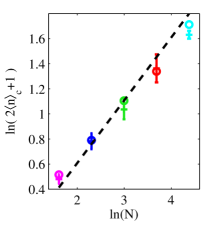
Figure 3: Number of photons at the critical coupling $\lambda=\lambda_{c}$, as a function of $N$, for a Dicke model with $\omega_{z}=2$, $\omega_{c}=\kappa=1$, and $\gamma=0$. Diagrammatic expansion (o), Monte-Carlo-wave-function method^{Mølmer et al. (1993); Vukics and Domokos (2012)} (+), and $\zeta=1/2$ critical scaling (dashed lines). Reproduced from Ref. Dalla Torre et al. (2013).

V.2 Fermionic diagrammatic expansion

An alternative method to obtain a controlled perturbative expansion in $1/N$ is given by the fermionic path integral approach^{Dalla Torre et al. (2016)}. The key idea is to describe each atomic degree of freedom using the Majorana fermion representation of spin-1/2^{Tsvelik (2007); Shnirman and Makhlin (2003); Schad et al. (2015)}. In this language the spin is replaced by a complex fermion $f$ and a Majorana fermion $\eta$. The former keeps track of the polarization of the spins $f^{\dagger}f=1/2-\sigma_{z}$, while the latter ensures the correct commutation relations are respected. This formalism allowed the authors of Ref. Dalla Torre et al. (2016) to develop a controlled $1/N$ expansion of the Dicke model. The key result was that to leading order in $1/N$, only one-loop diagrams (and their products) survive. These diagrams can be exactly resummed using the common Dyson resummation, i.e. by adding a self-energy contribution to the free Green’s function of the cavity: $[G_{a}^{R}]^{-1}\to[G_{a}^{R}]^{-1}+\Sigma_{a}^{R}$. Here $[G^{R}_{a}]^{-1}$ is the $2\times 2$ upper-left block of Eq. (21) and $\Sigma_{a}^{R}$ is a loop integral. Importantly, this expression simply corresponds to the spin-spin correlation function and can be written as

$$\Sigma_{a}^{R}(\omega)= -\frac{8\lambda^{2}}{N}\sum_{j=1}^{N}\int_{0}^{\infty}dt~{}{\rm{Im}}\left[{\langle\sigma^{x}_{j}(t)\sigma^{x}_{j}(0)\rangle}\right]e^{i\omega t}\;.$$ (44)

This result has a simple physical meaning: The coupling between the atoms and the cavity is proportional to $1/\sqrt{N}$. Thus, in the limit $N\to\infty$ the feedback of the cavity onto the atoms is negligible below threshold. As a consequence, the cavity feels the free evolution of the spins, and the superradiance transition is determined by a sum over $N$ independent terms. This result is analogous to the Lamb theory of lasing^{Lamb Jr (1964); Agarwal and Gupta (1990); Scully and Zubairy (1997); Gartner (2011)}, where the feedback of the cavity on the atoms is neglected (see Sec. VI for a discussion on the similarities and differences between superradiance and lasing).

The superradiant transition occurs when the dressed Green’s function has a pole at zero frequency, or

$${\rm det}\left[[G_{a}^{R}]^{-1}(0)+\Sigma_{a}^{R}(0)\right]=0$$ (45)

Substituting Eq. (44) in the expression for $[G_{a}^{R}]^{-1}$, we obtain the condition for the superradiant transition

$${\rm det}\left[\left(\begin{array}[]{c c}i\kappa-\omega_{c}+\Sigma_{a}^{R}(0)&\Sigma_{a}^{R}(0)\\ \Sigma_{a}^{R}(0)&-i\kappa-\omega_{c}+\Sigma_{a}^{R}(0)\end{array}\right)\right]=0\;,$$ (48)

where we used the fact that $\Sigma^{R}_{a}(0)$ is real by definition. A direct evaluation leads to

$$\omega^{2}_{c}+\kappa^{2}+2\omega_{c}\Sigma^{R}_{a}(0)=0\;,$$ (49)

This approach has two limiting cases that coincide with earlier results: (i) For a system at thermal equilibrium ${\langle\sigma^{z}\rangle}=(1/2)\tanh(\omega_{z}/2T)$ and $\gamma=0$. In this case, $\Sigma_{a}^{R}(0)=4\lambda^{2}{\langle\sigma^{z}\rangle}/\omega_{z}$, and we recover the equilibrium result, Eq. (9). (ii) In the presence of single-atom decay and dephasing

$${\langle\sigma^{x}_{j}(t)\sigma^{x}_{j}(0)\rangle}=e^{-\gamma_{T}t}\left[\cos(\omega_{z}t)+i{\langle\sigma^{z}\rangle}\sin(\omega_{z}t)\right]\;.$$ (50)

where $\gamma_{T}=\gamma_{\phi}+\gamma_{\downarrow}$. In this case, $\Sigma_{a}^{R}(0)=4\lambda^{2}{\langle\sigma^{z}_{j}\rangle}\omega_{z}/(\omega_{z}^{2}+\gamma^{2})$, and Eq. (49) becomes equivalent to Eq. (26).

In addition, the present diagrammatic approach allows us to consider inhomogeneous systems: Eq. (49) shows that the transition is governed by the disorder-averaged value of $\bar{\lambda}^{2}=(1/N)\sum_{j}\lambda_{j}^{2}$. One particular application is the case of inhomogeneous broadening when coupling to Raman transitions between hyperfine states, discussed by Ref. Zhiqiang et al. (2018). Furthermore, if the energy splitting of the two-level atoms is disordered, one sees this approach gives the $(\omega_{c}^{2}+\kappa^{2})/\omega_{c}=4\langle{\lambda_{i}^{2}}/\omega_{z,i}\rangle$. An application of this occurs when considering transitions between motional states of a thermal gas^{Piazza et al. (2013)}, for which the two-level system energy, $\omega_{zi}=\epsilon_{\boldsymbol{k}_{i}+\boldsymbol{Q}_{\text{recoil}}}-\epsilon_{\boldsymbol{k}_{i}}$ with $\epsilon_{\boldsymbol{k}}=\hbar^{2}k^{2}/2m$, depends on the Boltzmann distributed initial momentum of the atoms.

V.3 Cumulant expansion

A further way to consider systems with finite $N$ is to derive a hierarchy of coupled equations for all moments of the photon and spin operators. In the thermodynamic limit, $N\to\infty$, only the mean-field parts of these equations survive while at large but finite $N$ the second order correlation functions can give an accurate picture of the behavior.

When analyzing the dynamics using simply mean-field theory it is necessary to introduce symmetry breaking terms by hand. This is because the normal state is always a solution to the mean-field equations. By considering the second moments of the distribution one may look for discontinuities in quantities such as the photon number which respect the $\mathbb{Z}_{2}$ symmetry of the model. This allows us to only consider a reduced set of equations for the second moments which respect these symmetries. These techniques are closely related to those used in laser theory to describe the emergence of spontaneous coherence there^{Haken (1970, 1975)}.

For the Dicke model there are three distinct classes of these equations. The first are those that describe correlations of the photon mode

$$\partial_{t}\left\langle{a^{\dagger}a}\right\rangle =-2\kappa\left\langle{a^{\dagger}a}\right\rangle-\lambda N\operatorname{\mathrm{Im}}[C^{ax}]$$ (51)

$$\partial_{t}\left\langle{aa}\right\rangle =-2(i\omega_{c}+\kappa)\left\langle{aa}\right\rangle-i\lambda NC^{ax}$$ (52)

where we have denoted $C^{ax}=\left\langle{a\sigma^{x}}\right\rangle$. The second type of equations are those which involve correlations between the photon and spin degrees of freedom:

$$\begin{split}\partial_{t}C^{ax}=-\left(i\omega_{c}+\kappa+\gamma_{T}\right)C^{ax}-\omega_{z}C^{ay}\\ -i\lambda\left[\left(N-1\right)C^{xx}+\frac{1}{2}\right],\end{split}$$ (53)

$$\begin{split}\partial_{t}C^{ay}=-\left(i\omega_{c}+\kappa+\gamma_{T}\right)C^{ay}-\lambda\left\langle{\sigma^{z}}\right\rangle\left(\left\langle{aa}\right\rangle+\left\langle{a^{\dagger}a}\right\rangle\right)\\ +\omega_{z}C^{ax}-i\lambda\left[(N-1)C^{xy}-i\frac{1}{2}\left\langle{\sigma^{z}}\right\rangle\right].\end{split}$$ (54)

In these equations $C^{\alpha\beta}$ means $\langle\sigma^{\alpha}_{i}\sigma^{\beta}_{j\neq i}\rangle$ the correlation between $\sigma^{\alpha}$ at one site and $\sigma^{\beta}$ at another. All such correlations are equivalent since each atom is identical. These cross correlations obey:

$$\partial_{t}C^{xx} =-2\omega_{z}C^{xy}-2\gamma_{T}C^{xx},$$ (55)

$$\partial_{t}C^{yy} =2\omega_{z}C^{xy}-2\gamma_{T}C^{yy}-4\lambda\left\langle{\sigma^{z}}\right\rangle\operatorname{\mathrm{Re}}[C^{ay}],$$ (56)

$$\partial_{t}C^{zz} =4\lambda\left\langle{\sigma^{z}}\right\rangle\operatorname{\mathrm{Re}}[C^{ay}]-4\gamma_{\downarrow}\left(C^{zz}+\frac{1}{2}\left\langle{\sigma^{z}}\right\rangle\right),$$ (57)

$$\partial_{t}C^{xy} =\omega_{z}(C^{xx}-C^{yy})-2\gamma_{T}C^{xy}-2\lambda\left\langle{\sigma^{z}}\right\rangle\operatorname{\mathrm{Re}}[C^{ax}].$$ (58)

In writing these expression we have broken third order moments into products of first and second moments by assuming that the third order cumulants vanish. These equations do not put any restrictions on the types of decay processes which can be present and those written above include both collective decay channels such as photon loss and individual atomic loss and dephasing.

In most cases, the decay channels only shift the position of the transition. One important exception was found by Ref. Kirton and Keeling (2017), who showed that the presence of dephasing ($\gamma_{\phi}$) without losses ($\gamma_{\downarrow}=0$) completely suppresses the transition: This effect is demonstrated in Fig. 4, which shows the behavior at a value of the coupling far above the mean-field prediction for the location of the transition. This figure shows the reduced photon number (${\langle a^{\dagger}a\rangle}/N$), as a function of $N$, for various combinations of loss processes. In the case of $\gamma_{\downarrow}=0$, the dynamics always reaches a normal state with an average photon number that scales only as $\sqrt{N}$. This effect is due to the depolarization of the atoms due to sub-leading terms in the $1/N$ expansion, which can be compensated by decay processes ($\gamma_{\downarrow}\neq 0$) that polarize the atoms. As we will see below, this prediction is in good agreement with the numerical results obtained for finite $N$.

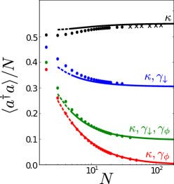
Figure 4: Number of photons for $\lambda>\lambda_{c}$, obtained from the cumulant expansion method (lines) and from the numerics (dots). The lines correspond, from top to bottom, to $\gamma_{\downarrow}=\gamma_{\phi}=0$ (black), $\gamma_{\downarrow}=0.1$, $\gamma_{\phi}=0$ (blue), $\gamma_{\downarrow}=0.1$, $\gamma_{\phi}=0.2$ (green) and $\gamma_{\downarrow}=0$, $\gamma_{\phi}=0.02$ (red). Other parameters are: $\lambda\sqrt{N}=0.9$, $\omega_{c}=1$, $\omega_{z}=1$, $\kappa=1/2$. Reproduced from Ref. Kirton and Keeling (2017).

V.4 Numerical approaches

For small numbers of atoms it is straightforward to find the exact Hamiltonian or Liouvillian of the appropriate model, determine the density operators in a thermal or steady-state ensemble, and calculate all possible observables. To reach larger system sizes it is possible to use the collective spin representation of the Dicke model as in Eq. (2). The Hilbert space dimension then scales linearly with the number of atoms and so the problem can again be straightforwardly diagonalized. This approach is, however, limited to only studying collective decay processes. More sophisticated methods are required to study the problem efficiently when individual loss processes are present.

In this more general case, a subtle symmetry can be exploited to efficiently calculate the behavior of the system. This remaining symmetry is a permutation symmetry at the level of the density matrix rather than in the Hilbert space: If the master equation can be written as a sum of processes where each term only affects a single site $i$, then swapping any pair of sites leaves the state unchanged. In this case, each element of the density matrix (ignoring the photon) must obey:

$$\bra{s^{L}_{1}\ldots s^{L}_{i}\ldots s_{j}^{L}\ldots s_{N}^{L}}\rho\ket{s^{R}_{1}\ldots s^{R}_{i}\ldots s_{j}^{R}\ldots s_{N}^{R}}$$

$$\equiv\bra{s^{L}_{1}\ldots s^{L}_{j}\ldots s_{i}^{L}\ldots s_{N}^{L}}\rho\ket{s^{R}_{1}\ldots s^{R}_{j}\ldots s_{i}^{R}\ldots s_{N}^{R}},$$

where $s^{L(R)}=\pm 1/2$. The full density matrix then separates into sets of permutation-symmetric elements. To find the dynamics of the system it is sufficient to propagate a single representative element from each of these sets, therefore gaining a combinatoric reduction to the size of the Liouvillian. The steady state can also be calculated by finding, in this restricted space, the eigenvector of the Liouvillian with eigenvalue 0.

This approach has been applied to a variety of problems which preserve this permutation symmetry. For example, it was used to study spin ensembles^{Chase and Geremia (2008)}, lasing models^{Xu et al. (2013)}, coherent surface plasmons^{Richter et al. (2015)}, the competition between collective and individual decay channels^{Damanet et al. (2016)}, the behavior of an ensemble of Rydberg polaritons^{Gong et al. (2016)}, equilibrium properties of a model with a larger local Hilbert space^{Zeb et al. (2018)}, subradiant states in the Dicke model^{Gegg et al. (2018)}, the effect of individual losses on transient superradiant emission^{Shammah et al. (2017)} and the crossover between superradiance and lasing^{Kirton and Keeling (2018)} (see Sec. VI.2). These results are reviewed in Ref. Shammah et al. (2018), while libraries which implement this method can be found at Refs. Kirton (2017); Gegg and Richter (2017); Shammah and Ahmed (2018).

This method was also applied to the Dicke model, to study the effect of individual loss processes on the superradiant transition. As shown in Fig. 4, the numerical results are in quantitative agreement with the above-mentioned cumulant expansion^{Kirton and Keeling (2017)}, valid for large $N$. Thus, a combination of these two methods is able to cover the entire range of number of atoms; from $N=1$ to $\infty$.

VI Superradiance and lasing

In this section we discuss the relation between the superradiance transition and lasing. To make this connection clear, in Sec. VI.1 we first discuss a canonical model of lasing, namely the Tavis–Cummings model. Next, in Sec. VI.2 we introduce a generalized Dicke model that interpolates between the Dicke and the Tavis–Cummings model. This family of models provides a link between the superradiant transition and the closely related phenomenon of lasing. In Secs. VI.3-VI.4, we describe different types of lasing transitions (regular lasing, counter lasing, and superradiant lasing) and explain their similarities and differences with the superradiant transition.

VI.1 The Tavis–Cummings model

The Tavis–Cummings model is given by a Dicke model without counter-rotating terms:

$$H=\omega_{c}a^{\dagger}a+\omega_{z}\sum_{j=1}^{N}\sigma^{z}_{j}+\frac{\lambda}{\sqrt{N}}\sum_{j=1}^{N}(a\sigma^{+}_{j}+a\sigma^{-}_{j})$$ (59)

This model conserves the total number of excitations $N_{\text{ex}}=a^{\dagger}a+\sum_{j}\sigma^{z}_{j}$. This symmetry is associated with a $U(1)$ gauge symmetry $a\to e^{i\phi}a$ and $\sigma^{-}\to e^{i\phi}\sigma^{-}$. The equilibrium Tavis–Cummings model has a phase transition at $\lambda=\sqrt{\omega_{c}\omega_{z}}$, where the symmetry is spontaneously broken. This critical coupling differs by a factor of two from the Dicke result, as only half the matter-light coupling terms are present.

In the presence of decay, the Tavis–Cummings model does not show a superradiant transition^{Keeling et al. (2010); Larson and Irish (2017); Soriente et al. (2018)}. This result has a simple physical meaning: because the model does not have counter-rotating terms, it will always flow to a trivial steady state, where the cavity is empty and the spins are polarized in the $\sigma^{z}=-1/2$ direction. The superradiant transition occurs only if the total number of excitations is kept constant (when no loss processes are present). The Tavis–Cummings model can nevertheless show a lasing transition if the atoms are pumped. In what follows, we explain the difference between the superradiant transition and the lasing transition, by considering a simple model in which both transitions occur.

VI.2 Generalized Dicke model

The generalized Dicke model is a simple interpolation between the Dicke model (1) and the Tavis–Cummings model (59),

$$H=\omega_{c}a^{\dagger}a+\omega_{z}\sum_{j=1}^{N}\sigma_{j}^{z} +\frac{\lambda}{\sqrt{N}}\sum_{j=1}^{N}(a\sigma^{+}_{j}+a^{\dagger}\sigma^{-}_{j})$$

$$+\frac{\lambda^{\prime}}{\sqrt{N}}\sum_{j=1}^{N}(a\sigma^{-}_{j}+a^{\dagger}\sigma^{+}_{j})\;.$$ (60)

This model includes the Dicke model ($\lambda=\lambda^{\prime}$) and the Tavis–Cummings model ($\lambda^{\prime}=0$) as special cases. It can be realized using the 4-level scheme described in Sec. II, where rotating and counter-rotating terms are induced by two separate pumping fields.

Using the Holstein–Primakoff approximation^{Holstein and Primakoff (1940)}, one can map this model to two coupled harmonic oscillators:

$$H=\omega_{c}a^{\dagger}a+\omega_{z}b^{\dagger}b+\lambda(ab^{\dagger}+a^{\dagger}b)+\lambda^{\prime}(ab+a^{\dagger}b^{\dagger})\;.$$ (61)

This Hamiltonian can be represented as a $4\times 4$ matrix

$$H=\frac{1}{2}(a~{}a^{\dagger}~{}b~{}b^{\dagger})\left(\begin{array}[]{c c c c}\omega_{c}&0&\lambda&\lambda^{\prime}\\ 0&\omega_{c}&\lambda^{\prime}&\lambda\\ \lambda&\lambda^{\prime}&\omega_{z}&0\\ \lambda^{\prime}&\lambda&0&\omega_{z}\end{array}\right)\left(\begin{array}[]{c}a^{\dagger}\\ a\\ b^{\dagger}\\ b\end{array}\right)$$ (62)

where $\lambda_{\pm}=\lambda\pm\lambda^{\prime}$. Following the same analysis as in Sec. III.2 one obtains

$$G_{R}^{-1}=\left(\begin{array}[]{c c c c}\omega-\omega_{c}+i\kappa&0&-\lambda&-\lambda^{\prime}\\ 0&-\omega-\omega_{c}-i\kappa&-\lambda^{\prime}&-\lambda\\ -\lambda&-\lambda^{\prime}&\omega-\omega_{z}&0\\ -\lambda^{\prime}&-\lambda&0&-\omega-\omega_{z}\end{array}\right)$$ (63)

where $\kappa$ is the cavity decay rate. The superradiant transition is signaled by ${\rm det}[G_{R}^{-1}(\omega=0)]=0$, or

$$(\lambda^{2}-\lambda^{\prime 2})^{2}-2(\lambda^{2}+\lambda^{\prime 2})\omega_{c}\omega_{z}+(\kappa^{2}+\omega_{c}^{2})\omega_{z}^{2}=0$$ (64)

Let us now consider the two above-mentioned limiting cases: in the Dicke model ($\lambda=\lambda^{\prime}$), one recovers Eq. (22). In contrast, for the Tavis–Cummings model ($\lambda^{\prime}=0$). the superradiant transition occurs for

$$(\lambda^{2}-\omega_{c}\omega_{z})^{2}+\kappa^{2}\omega_{z}^{2}=0.$$ (65)

This condition cannot be satisfied for any $\kappa\neq 0$, in agreement with the results of Sec. VI.1. In general, for any finite $\kappa$, the critical coupling diverges when approaching the TC limit of $\lambda^{\prime}\to 0$^{Keeling et al. (2010)}. It is worth also noting that identical behavior occurs if we set $\lambda=0$ and consider the model with only only counter-rotating terms. In fact this limit is also the Tavis-Cummings model after a unitary transform, rotating the spin by $\pi$ about the $x$ axis, thus sending $\sigma^{\pm}\to\sigma^{\mp}$ and $\sigma^{z}\to-\sigma^{z}$.

When considering the full phase diagram of dissipative Dicke model with $\lambda\neq\lambda^{\prime}$, some new features can arise. In particular there exists a phase where both the normal state and superradiant state are stable, and a multicritical point where this phase vanishes, as has been reported a number of times^{Keeling et al. (2010); Soriente et al. (2018); Gutiérrez-Jáuregui and Carmichael (2018)}.

VI.3 Regular and counter-lasing transitions

Although the Tavis–Cummings model cannot undergo a superradiant transition, this model can describe the transition to a lasing state^{Scully and Zubairy (1997)}. We first discuss how this distinct form of coherent light arises in this model, before considering how the lasing state and superradiant states can be related and distinguished. To obtain lasing, it is sufficient to supplement the TC model, Eq. (59), by an incoherent driving term that pumps the atoms in the excited state. This effect can be described by adding a Lindblad operator to Eq. (4) where $L=\sigma^{+}$ with a rate $\gamma_{\uparrow}$. This process is directly analogous to a three-level model of a laser, where one of the levels is pumped incoherently, leading to population inversion. The resulting phase transition leads to a lasing state, rather than a superradiant state.

The relation of lasing and superradiance is made clear if one considers the generalized Dicke model (with $\lambda^{\prime}\neq\lambda$) combined with the incoherent pumping discussed above^{Kirton and Keeling (2018)}. In this case, one sees two distinct ordered states: a lasing state that continuously connects to the state with $\lambda^{\prime}=0$, and a superradiant state that connects to the Dicke model with $\lambda^{\prime}=\lambda,\gamma_{\uparrow}=0$. These two states occupy disconnected regions on the $\lambda^{\prime},\gamma_{\uparrow}$ phase diagram – see Fig. 5. From a physical perspective, the lasing and superradiant transitions can be clearly distinguished as lasing only occurs when ${\langle\sigma^{z}\rangle}>0$, while the superradiant state occurs only for ${\langle\sigma^{z}\rangle}<0$^{Kirton and Keeling (2018)}.

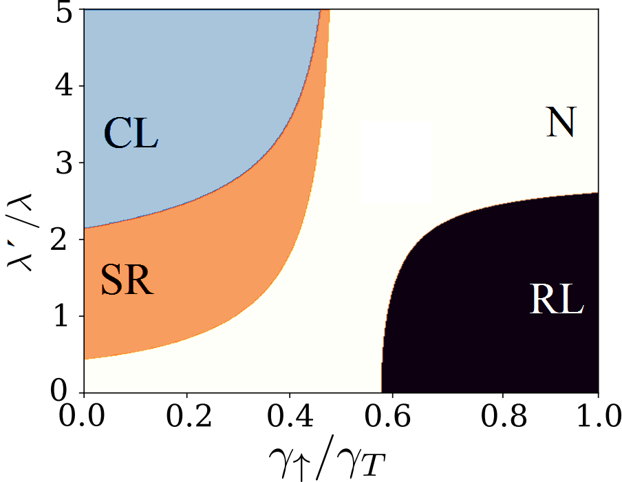
Figure 5: Phase diagram of the generalized Dicke model, Eq. (60), with repumping $\gamma_{\uparrow}$. This model shows regions of superradiance (SR), counter-lasing (CL), and regular lasing (RL). A normal (N) region separates the regions without population inversion (SR and CL) from the regular lasing region. Numerical parameters: $\omega_{z}=1,~{}\omega_{0}=1,~{}\lambda=0.9,\kappa=0.5,~{}\gamma_{T}=0.5$. Adapted from Ref. Kirton and Keeling (2018).

In addition to the presence or absence of inversion, the lasing and superradiant phases have a different nature: In the superradiant phase the field is locked to the rotating frame of the pump. In contrast, in a lasing phase, the coherent emission is not locked to the pump frequency and is time dependent in the frame of the pump. From a mathematical perspective the Dicke transition corresponds to a subcritical pitchfork instability, where a single eigenvalue vanishes^{Strogatz (2018)}. In contrast, the lasing transition corresponds to a critical Hopf bifurcation, i.e. to a point where two eigenvalues become unstable simultaneously, by crossing the real axis without passing through the origin. Because the unstable modes have a finite real part, this transition generically leads to oscillations. Other examples of Hopf bifurcations in generalized Dicke models were predicted by Ref. Bhaseen et al. (2012) and Ref. Genway et al. (2014), who considered the effects of additional terms, such as $US_{z}^{2}$ and $\Omega S_{x}$. When the instability is crossed, the system generically gives rise to oscillating superradiant phases, described by limit cycles ^{Bhaseen et al. (2012); Piazza and Ritsch (2015)}.

In addition to standard lasing for the inverted state, a lasing instability can alternatively be obtained for the Dicke model with negative detuning of the cavity ($\omega_{c}<0$), where the superradiant transition does not occur^{Klinder et al. (2015); Zhiqiang et al. (2018)}. Moreover, even in the absence of incoherent pumping (${\langle\sigma^{z}\rangle}<0$) and for positive cavity detunings ($\omega_{c}>0$), a lasing transition can be obtained in the generalized Dicke model of Sec. VI.2. This transition occurs when the counter-rotating terms lead to a coherent emission of photons from the cavity. It was termed the “inverted-lasing”^{Kirton and Keeling (2018)} or “counter-lasing”^{Shchadolova et al. (2018)} transition and had been observed experimentally by Zhiqiang et al.^{Zhiqiang et al. (2017)}, see Fig. 6.

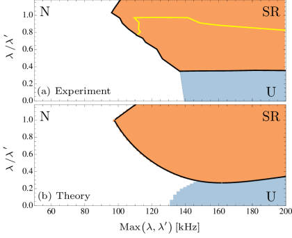
Figure 6: Comparison between (a) experimental and (b) theoretical phase diagrams for the generalized Dicke system, Eq. (60), in the absence of repumping. The system can be either normal (N), superradiant (SR), or unstable/counter-lasing (U). The SR regime below the yellow line shows transient oscillations in time and is possibly related to the oscillating superradiance of Ref. Bhaseen et al. (2012). The parameters used for theoretical calculation correspond to the experimental values: cavity mode frequency $\omega_{c}=100$ kHz, dissipation $\kappa=107$ kHz, and energy splitting $\omega_{z}=77$kHz. The atomic polarization is assumed to be ${\langle\sigma^{z}\rangle}=-0.25$ and the dissipation $\gamma_{T}=30$kHz. Reproduced from Ref. Shchadolova et al. (2018).

VI.4 Superradiant lasers

As noted above, the Tavis–Cummings model with incoherent pumping can undergo a transition to a coherent state, i.e. lasing. The connection between this transition and the transient superradiance discussed by Dicke has been considered a number of times^{Kolobov et al. (1993); Haake et al. (1993); Meiser et al. (2009); Meiser and Holland (2010)}. As mentioned in Sec. I, in the absence of a cavity, transient superradiance produces a coherent pulse by effectively synchronizing the emission of all atoms through the collective decay process. By placing many atoms in a bad cavity, and continuously incoherently repopulating the excited state, one may try to drive a continuous superradiance process, which has been termed a superradiant laser^{Haake et al. (1993)}. Such a device based on atomic transitions can boast a very narrow linewidth, determined by the sharply defined atomic resonance frequency, rather than the cavity. If one uses a suppressed electronic transition for the lasing level, this allows a very small natural linewidth $\gamma$, but yet superradiant lasing can emerge in the collective strong coupling regime, $N\lambda^{2}\gg\kappa\gamma$. Moreover, the linewidth at peak lasing power scales as $N^{-2}$; this suggests a potential mHz linewidth from $10^{6}$ atoms, a level that could significantly improve atomic clock accuracies^{Meiser et al. (2009)}.

Earlier works^{Haake et al. (1993)} were based on a three-level lasing scheme, and did not address how superradiant lasing arises in the presence of individual decay and dephasing of the atoms. A simpler two-level description was given in Refs. Meiser et al. (2009); Meiser and Holland (2010), using the cumulant expansion approach described in Sec. V.3. Such a superradiant laser has been realized experimentally, in a scheme where the lasing transition was actually a two photon Raman transition^{Bohnet et al. (2012a, b)}, enabling tuning of both the matter light coupling $\lambda$ and the effective natural linewidth $\gamma$ of the transition.

VII Closely related models

So far in this review, we have focused on the Dicke model, as well as the generalized Dicke model in which we allow distinct strengths of the rotating and counter-rotating terms. There do however exist a number of models that are closely related to the Dicke model, involving coupling between many two-level systems and a common cavity mode, as well as models such as the Rabi model that can be shown to have a close connection to superradiance. Here we provide a brief summary of these models, and the novel physics they can introduce.

VII.1 Extended Dicke models

The Raman driving scheme used to realize the Dicke model generates additional terms that need to be taken into account. In particular, the difference between the cavity-photon-induced Stark shifts in the two atomic states leads to a term $Ua^{\dagger}a\sigma^{z}$. This term can also be seen as a modification of the cavity frequency depending on the atomic state. For the motional state realization, such a term is inevitable (due to the different overlaps between the two momentum states with the cavity optical lattice)^{Nagy et al. (2010); Baumann et al. (2010)}. For the Raman realization, the strength of $U$ can in principle be turned to zero^{Dimer et al. (2007)}. Such a term has been studied extensively in Ref. Bhaseen et al. (2012), where it was seen to enable bistability between normal and superradiant states, as well as distinct superradiant states and time-dependent attractors, i.e. limit cycles.

Another additional term that can be easily engineered is a drive, $H_{F}=F(a+a^{\dagger})$, which corresponds to a coherent light source coupled directly to the cavity mode. This term has the same physical effect as $H_{F}^{\prime}=F\sigma_{x}$, these two forms being related by a unitary transformation. This latter term arises naturally in many realizations of the Dicke model using trapped ions^{Porras and Cirac (2004); Wang et al. (2013); Genway et al. (2014); Pedernales et al. (2015); Aedo and Lamata (2018)}. These two terms break the $\mathbb{Z}_{2}$ symmetry of the Dicke model, and thus destroy the phase transition. However, there can still be optical bistability^{Bowden and Sung (1979)} between a high field and low field state, i.e. the open-system analog of a first order phase transition. The behavior of this model at large driving has also been recently discussed in Ref. Gutiérrez-Jáuregui and Carmichael (2018), establishing the connection to breakdown of the photon blockade seen in the single-atom Jaynes-Cummings model^{Carmichael (2015)}.

VII.2 Disordered Dicke model

The above models involve adding extra terms to the Dicke model; another class of closely related models involves considering the role of disorder. i.e., returning to Eq. (1) in terms of individual two-level systems, and allowing different energies or coupling strengths for different systems:

$$H=\omega_{c}a^{\dagger}a+\sum_{j=1}^{N}\omega_{z}^{j}\sigma^{z}_{j}+\frac{2}{\sqrt{N}}(a+a^{\dagger})\sum_{j}\lambda^{j}\sigma^{x}_{j}\;.$$ (66)

Such models have been studied in a wider variety of contexts, including the effects of disorder on dynamical superradiance in a low Q cavity^{Temnov and Woggon (2005)}, the phase diagram of microcavity polaritons^{Marchetti et al. (2006, 2007)}, solid state quantum memories^{Diniz et al. (2011)}, as well as for cold atom in optical cavities, accounting for the spatial variation of the cavity modes^{Zhiqiang et al. (2018)}. Several works in this context have investigated the dynamics of an initially prepared state, using either brute force numerics for small systems^{Tsyplyatyev and Loss (2009); Krimer et al. (2014, 2016)}, or matrix product state approaches^{Dhar et al. (2018)}. The existence of such disorder prevents the simplification of replacing individual spins by a collective spin operator, hence the need for efficient numerical methods to explore this enlarged Hilbert space^{Dhar et al. (2018)}. It is however notable that in the case where $\omega^{j}_{z}$ is disordered, while $\lambda^{j}=\lambda$, the model can be shown to be integrable, as a special case of a Richardson-Gaudin model^{Dukelsky et al. (2004); Kundu (2004); Tschirhart and Faribault (2014); Yuzbashyan (2018)}. In addition to the dynamics, one can also calculate the phase diagram of the disordered Dicke model by mean-field approaches^{Marchetti et al. (2006, 2007)}, showing that the disorder does not destroy the superradiant phase, but modifies the phase boundary.

VII.3 Floquet Dicke models

Another class of driven-dissipative generalized Dicke models involve time dependent couplings. In particular, Floquet-Dicke models where $\lambda(t)=\lambda_{0}+\Delta\lambda\cos(\Omega t)$ have been considered^{Bastidas et al. (2012)}. These models show a complex phase diagram, depending on the ratio of the drive frequency to other energy scales in the model. Recent work on the same model has studied how time dependent driving can suppress the formation of the superradiant state^{Cosme et al. (2018)}.

VII.4 Scaling limit of the Rabi model

We finally consider a model that has a quite different structure to the Dicke model, but nonetheless can show a similar superradiance transition. This is the Rabi model, describing the coupling between a quantized harmonic oscillator and a single spin:

$$H=\omega_{c}a^{\dagger}a+\omega_{z}\sigma^{z}+2\lambda(a+a^{\dagger})\sigma^{x}\;.$$ (67)

To observe the superradiant transition in this model, Hwang et al.^{Hwang et al. (2015, 2018)} proposed considering the limit in which the atomic splitting $\omega_{z}$ tends to infinity. This limit can be formally studied by defining $\omega_{z}=\eta\tilde{\omega}_{z},\lambda=\tilde{\lambda}\sqrt{\eta}$ and considering the limit of $\eta\to\infty$ such that $\lambda^{2}/(\omega_{c}\omega_{z})$ remains finite. If one considers the mean field ansatz of Sec. III.1, one finds the ground state free energy $F(\alpha)=\omega_{c}\alpha^{2}-{\color[rgb]{0,0,0}{\frac{1}{2}}}\sqrt{\eta^{2}\tilde{\omega}_{z}^{2}+{\color[rgb]{0,0,0}{16}}\eta\tilde{\lambda}^{2}\alpha^{2}}.$ In order to consider the limit $\eta\to\infty$, it is convenient to consider $\alpha=\sqrt{\eta}x$ which gives:

$$F(x)=\eta\left[\omega_{c}x^{2}-{\color[rgb]{0,0,0}{\frac{1}{2}}}\sqrt{\tilde{\omega}_{z}^{2}+16\tilde{\lambda}^{2}x^{2}}\right].$$ (68)

This expression is equivalent to the $T=0$ form of Eq. (8) with $\eta$ playing the role of the number of atoms. In the limit $\eta\to\infty$, there is a sharp phase transition at $\tilde{\lambda}=\sqrt{\tilde{\omega}_{z}\omega_{c}}/2$, analogous to the Dicke model.

The phase transition of this model can also be found by adiabatically eliminating the state of the two-level system using a Schrieffer-Wolff transformation, leading to an effective photon-only problem

$$H=-{\color[rgb]{0,0,0}{\frac{\omega_{z}}{2}}}+\omega_{c}a^{\dagger}a-\frac{\lambda^{2}}{\omega_{z}}(a+a^{\dagger})^{2}$$ (69)

After a Bogoliubov transformation, this expression gives a photon frequency, $\sqrt{\omega_{c}(\omega_{c}-4\lambda^{2}/\omega_{z})}$, which vanishes at the transition.

VIII Conclusion

The Dicke model is one of the fundamental models of cavity quantum electro-dynamics (cavity-QED), describing the coupling of many atoms to a single cavity mode. The thermodynamic limit of this model is achieved by considering an infinite number of atoms, whose coupling to the cavity tends to zero. This model can undergo a phase transition to a superradiant state at a critical value of the light-matter coupling. Various physical realizations of this model have been considered, which may be thought of as analog quantum simulators of the Dicke model, built from driven atoms in cavities, superconducting qubits, or trapped ions. In this Progress Report, we introduced the reader to the equilibrium and non-equilibrium behavior of this model and showed how to calculate the critical properties of the superradiant transition. For simplicity, we focused on the simplest realization of the Dicke model where mean-field theory gives a good understanding of the behavior. Our discussion focused on the theoretical aspects of the transition. Experiments were able to probe a diverging susceptibility at the transition^{Landig et al. (2015)}, but the critical exponents were not found to match the theoretical expectations^{Brennecke et al. (2013)}. This point certainly deserves further investigation.

A natural generalization of this model involves two coupled cavity modes, leading to a competition between two superradiant phases. At the interface between these two phases the model shows an enlarged $U(1)$ symmetry^{Fan et al. (2014); Baksic and Ciuti (2014)}, as realized experimentally recently^{Léonard et al. (2017a, b)}. Such experiments have prompted theoretical discussion of the possibility of a vestigial ordered phase^{Gopalakrishnan et al. (2017)}, where the two cavities become phase locked but without superradiance, as well as the nature of the excitations close to the $U(1)$ symmetric point^{Lang et al. (2017)}. A further extension in this direction leads to multi-mode cavities, which give rise to spatially varying, cavity-mediated interactions among the atoms ^{Kollár et al. (2015, 2017); Vaidya et al. (2018)}. This system may lead to critical behavior beyond a mean field description^{Gopalakrishnan et al. (2009, 2010)}, give rise to new glassy phases^{Gopalakrishnan et al. (2011); Strack and Sachdev (2011); Buchhold et al. (2013); Rotondo et al. (2015)}, and have potential applications for memory storage^{Gopalakrishnan et al. (2012); Torggler et al. (2017)} and optimization problems^{Torggler et al. (2018)}.

The analysis of driven dissipative Dicke model raises many interesting questions. For example, the zero-temperature Dicke model was considered by Emary and Brandes^{Emary and Brandes (2003a, b)} in the framework of classical and quantum chaos. These authors found that the Dicke model (but not the Tavis–Cummings model) has a sharp transition between regular and chaotic motion. Interestingly, in the limit of large $N$, the position of the onset of chaos coincides with the quantum phase transition. The relation between quantum chaos and thermalization in the Dicke model was studied for example by Refs. Lambert et al. (2009); Altland and Haake (2012a, b); Bakemeier et al. (2013); Dalla Torre (2017). To fully access the chaotic regime, it is necessary to go beyond the linear stability analysis reviewed in this report. In addition to the critical behavior of the open Dicke model discussed in this review, other works have analyzed the behavior of this model from alternate perspectives, such as quantum information approaches^{Dey et al. (2012)}, large deviation approaches and the $s$-ensemble^{Rotondo et al. (2018)}, and fluctuation-dissipation relations^{Mur-Petit et al. (2018)}.

As we have shown, despite its long history, the Dicke model has continued to reveal new insights about the relation of phase transitions in equilibrium and driven systems. As a paradigmatic model of many body quantum optics, it continues to play an important role in framing discussions of collective behavior. Given the variety of different directions currently studied experimentally and theoretically, it is likely new understanding will continue to arise from this field in the future.

Acknowledgments We would like to thank Qing-Hu Chen, Sebastian Diehl, Peter Domokos, Tobias Donner, Andreas Hemmerich, Benjamin Lev, Francesco Piazza, Peter Rabl, and Nathan Shammah for reading an earlier version of this manuscript and giving important comments. P.K. acknowledges support from EPSRC (EP/M010910/1) and the Austrian Academy of Sciences (ÖAW). P.K. and J.K. acknowledge support from EPSRC program “Hybrid Polaritonics” (EP/M025330/1). M.M.R. and E.G.D.T. are supported by the Israel Science Foundation Grant No. 1542/14.

Appendix A Equations of motion and retarded Green’s functions

In this appendix we show how to obtain the retarded Green’s functions of a set of operators, starting from their Heisenberg equations of motion. Our approach applies to equations of motion given by the linear relation,

$$\dot{\boldsymbol{v}}(t)= M\boldsymbol{v}(t),$$ (70)

Our goal is to find the corresponding retarded Green’s function, defined by

$$G^{R}_{i,j}(t)= {-}i\left\langle{\left[v_{i}^{\vphantom{\dagger}}(t),v_{j}^{\dagger}(0)\right]}\right\rangle\theta(t).$$ (71)

We denote the equal-time correlation functions of these operators by a constant matrix $S_{i,j}=\left\langle{\left[v_{i}^{\vphantom{\dagger}}(0),v_{j}^{\dagger}(0)\right]}\right\rangle$. In terms of this matrix, we may write:

$$\partial_{t}G^{R}_{i,j}(t)=-i\delta(t)S_{i,j}+M_{i,k}G^{R}_{k,j}(t).$$ (72)

By defining the Fourier transform as

$$f(\omega)=\int\limits_{-\infty}^{\infty}\mathrm{d}t\,e^{i\omega t}f(t),$$

we can write Eq. (72) in the matrix form

$$({M}+i\omega\mathbbm{1}){G}^{R}(\omega)=i{S}.$$

This equations can be explicitly inverted to give

$$G^{R}(\omega)= \left[\omega{\mathbbm{1}}-iM\right]^{-1}S.$$ (73)

This expression gives a general connection between the linear equations of motions for a set of operators, and the retarded Green’s function for the same set of operators. Note that this expression is valid as long as the equal-time commutators, $S_{i,j}$, are constant in time.

References

- Dicke (1954) R. H. Dicke, Coherence in Spontaneous Radiation Processes, Phys. Rev. 93, 99 (1954).
- Hepp and Lieb (1973) K. Hepp and E. H. Lieb, Equilibrium statistical mechanics of matter interacting with the quantized radiation field, Phys. Rev. A 8, 2517 (1973).
- Wang and Hioe (1973) Y. K. Wang and F. T. Hioe, Phase Transition in the Dicke Model of Superradiance, Phys. Rev. A 7, 831 (1973).
- Hioe (1973) F. Hioe, Phase transitions in some generalized Dicke models of superradiance, Phys. Rev. A 8, 1440 (1973).
- Carmichael et al. (1973) H. Carmichael, C. Gardiner, and D. Walls, Higher order corrections to the Dicke superradiant phase transition, Phys. Lett. A 46, 47 (1973).
- Duncan (1974) G. C. Duncan, Effect of antiresonant atom-field interactions on phase transitions in the Dicke model, Phys. Rev. A 9, 418 (1974).
- Dimer et al. (2007) F. Dimer, B. Estienne, A. S. Parkins, and H. J. Carmichael, Proposed realization of the Dicke-model quantum phase transition in an optical cavity QED system, Phys. Rev. A 75, 013804 (2007).
- Zhiqiang et al. (2017) Z. Zhiqiang, C. H. Lee, R. Kumar, K. Arnold, S. J. Masson, A. Parkins, and M. Barrett, Nonequilibrium phase transition in a spin-1 Dicke model, Optica 4, 424 (2017).
- Domokos and Ritsch (2002) P. Domokos and H. Ritsch, Collective Cooling and Self-Organization of Atoms in a Cavity, Phys. Rev. Lett. 89, 253003 (2002).
- Black et al. (2003) A. T. Black, H. W. Chan, and V. Vuletić, Observation of Collective Friction Forces due to Spatial Self-Organization of Atoms: From Rayleigh to Bragg Scattering, Phys. Rev. Lett. 91, 203001 (2003).
- Nagy et al. (2010) D. Nagy, G. Kónya, G. Szirmai, and P. Domokos, Dicke-Model Phase Transition in the Quantum Motion of a Bose-Einstein Condensate in an Optical Cavity, Phys. Rev. Lett. 104, 130401 (2010).
- Baumann et al. (2010) K. Baumann, C. Guerlin, F. Brennecke, and T. Esslinger, Dicke quantum phase transition with a superfluid gas in an optical cavity, Nature 464, 1301 (2010).
- Klinder et al. (2015) J. Klinder, H. Keßler, M. Wolke, L. Mathey, and A. Hemmerich, Dynamical phase transition in the open Dicke model, Proc. Nat. Acad. Sci. 112, 3290 (2015).
- Vaidya et al. (2018) V. D. Vaidya, Y. Guo, R. M. Kroeze, K. E. Ballantine, A. J. Kollár, J. Keeling, and B. L. Lev, Tunable-Range, Photon-Mediated Atomic Interactions in Multimode Cavity QED, Phys. Rev. X 8, 011002 (2018).
- Nagy et al. (2011) D. Nagy, G. Szirmai, and P. Domokos, Critical exponent of a quantum-noise-driven phase transition: The open-system Dicke model, Phys. Rev. A 84, 043637 (2011).
- Öztop et al. (2012) B. Öztop, M. Bordyuh, O. E. Müstecaplioğlu, and H. E. Türeci, Excitations of optically driven atomic condensate in a cavity: theory of photodetection measurements, New J. Phys. 14, 085011 (2012).
- Dalla Torre et al. (2013) E. G. Dalla Torre, S. Diehl, M. D. Lukin, S. Sachdev, and P. Strack, Keldysh approach for nonequilibrium phase transitions in quantum optics: Beyond the Dicke model in optical cavities, Phys. Rev. A 87, 023831 (2013).
- Mezzacapo et al. (2014) A. Mezzacapo, U. Las Heras, J. Pedernales, L. DiCarlo, E. Solano, and L. Lamata, Digital quantum Rabi and Dicke models in superconducting circuits, Sci. Rep. 4, 7482 (2014).
- Lamata (2017) L. Lamata, Digital-analog quantum simulation of generalized Dicke models with superconducting circuits, Sci. Rep. 7, 43768 (2017).
- Aedo and Lamata (2018) I. Aedo and L. Lamata, Analog quantum simulation of generalized Dicke models in trapped ions, Phys. Rev. A 97, 042317 (2018).
- Keeling et al. (2010) J. Keeling, M. J. Bhaseen, and B. D. Simons, Collective Dynamics of Bose-Einstein Condensates in Optical Cavities, Phys. Rev. Lett. 105, 043001 (2010).
- Gross and Haroche (1982) M. Gross and S. Haroche, Superradiance: An essay on the theory of collective spontaneous emission, Phys. Rep. 93, 301 (1982).
- Garraway (2011) B. M. Garraway, The Dicke model in quantum optics: Dicke model revisited, Philos. Trans. Royal Soc. A 369, 1137 (2011).
- Ritsch et al. (2013) H. Ritsch, P. Domokos, F. Brennecke, and T. Esslinger, Cold atoms in cavity-generated dynamical optical potentials, Rev. Mod. Phys. 85, 553 (2013).
- Chen et al. (2008) Q.-H. Chen, Y.-Y. Zhang, T. Liu, and K.-L. Wang, Numerically exact solution to the finite-size Dicke model, Phys. Rev. A 78, 051801 (2008).
- Piazza et al. (2013) F. Piazza, P. Strack, and W. Zwerger, Bose–Einstein condensation versus Dicke–Hepp–Lieb transition in an optical cavity, Ann. Phys. 339, 135 (2013).
- Bhaseen et al. (2012) M. J. Bhaseen, J. Mayoh, B. D. Simons, and J. Keeling, Dynamics of nonequilibrium Dicke models, Phys. Rev. A 85, 013817 (2012).
- Scully and Zubairy (1997) M. O. Scully and M. S. Zubairy, Quantum Optics (Cambridge University Press, 1997).
- Dalla Torre et al. (2016) E. G. Dalla Torre, Y. Shchadilova, E. Y. Wilner, M. D. Lukin, and E. Demler, Dicke phase transition without total spin conservation, Phys. Rev. A 94, 061802 (2016).
- Kirton and Keeling (2017) P. Kirton and J. Keeling, Suppressing and restoring the Dicke superradiance transition by dephasing and decay, Phys. Rev. Lett. 118, 123602 (2017).
- Zhiqiang et al. (2018) Z. Zhiqiang, C. H. Lee, R. Kumar, K. Arnold, S. J. Masson, A. Grimsmo, A. Parkins, and M. Barrett, Dicke model simulation via cavity-assisted Raman transitions, (2018), 1801.07888 .
- Rzażewski et al. (1975) K. Rzażewski, K. Wódkiewicz, and W. Żakowicz, Phase transitions, two-level atoms, and the A 2 term, Phys. Rev. Lett. 35, 432 (1975).
- Bialynicki-Birula and Rzażewski (1979) I. Bialynicki-Birula and K. Rzażewski, No-go theorem concerning the superradiant phase transition in atomic systems, Phys. Rev. A 19, 301 (1979).
- Keeling (2007) J. Keeling, Coulomb interactions, gauge invariance, and phase transitions of the Dicke model, J. Phys. 19, 295213 (2007).
- Vukics and Domokos (2012) A. Vukics and P. Domokos, Adequacy of the Dicke model in cavity QED: A counter-no-go statement, Phys. Rev. A 86, 053807 (2012).
- Vukics et al. (2014) A. Vukics, T. Grießer, and P. Domokos, Elimination of the -Square Problem from Cavity QED, Phys. Rev. Lett. 112, 073601 (2014).
- Vukics et al. (2015) A. Vukics, T. Grießer, and P. Domokos, Fundamental limitation of ultrastrong coupling between light and atoms, Phys. Rev. A 92, 043835 (2015).
- Grießer et al. (2016) T. Grießer, A. Vukics, and P. Domokos, Depolarization shift of the superradiant phase transition, Phys. Rev. A 94, 033815 (2016).
- De Bernardis et al. (2018a) D. De Bernardis, T. Jaako, and P. Rabl, Cavity quantum electrodynamics in the nonperturbative regime, Phys. Rev. A 97, 043820 (2018a).
- De Bernardis et al. (2018b) D. De Bernardis, P. Pilar, T. Jaako, S. De Liberato, and P. Rabl, Breakdown of gauge invariance in ultrastrong-coupling cavity QED, arXiv:1805.05339 (2018b), 1805.05339 .
- Stokes and Nazir (2018) A. Stokes and A. Nazir, Gauge ambiguities in ultrastrong-coupling QED: the Jaynes-Cummings model is as fundamental as the Rabi model, arXiv:1805.06356 (2018), 1805.06356 .
- Flick et al. (2017) J. Flick, M. Ruggenthaler, H. Appel, and A. Rubio, Atoms and molecules in cavities, from weak to strong coupling in quantum-electrodynamics (QED) chemistry, Proc. Natl. Acad. Sci. 114, 3026 (2017).
- Rokaj et al. (2018) V. Rokaj, D. M. Welakuh, M. Ruggenthaler, and A. Rubio, Light–matter interaction in the long-wavelength limit: no ground-state without dipole self-energy, J. Phys. B 51, 034005 (2018).
- Eastham and Littlewood (2000) P. Eastham and P. Littlewood, Bose condensation in a model microcavity, Solid State Commun. 116, 357 (2000).
- Eastham and Littlewood (2001) P. R. Eastham and P. B. Littlewood, Bose condensation of cavity polaritons beyond the linear regime: The thermal equilibrium of a model microcavity, Phys. Rev. B 64, 235101 (2001).
- Deng et al. (2010) H. Deng, H. Haug, and Y. Yamamoto, Exciton-polariton Bose-Einstein condensation, Rev. Mod. Phys. 82, 1489 (2010).
- Carusotto and Ciuti (2013) I. Carusotto and C. Ciuti, Quantum fluids of light, Rev. Mod. Phys. 85, 299 (2013).
- Kasprzak et al. (2006) J. Kasprzak, M. Richard, S. Kundermann, A. Baas, P. Jeambrun, J. M. J. Keeling, F. M. Marchetti, M. H. Szymanska, R. André, J. L. Staehli, V. Savona, P. B. Littlewood, B. Deveaud, and L. S. Dang, Bose-Einstein condensation of exciton polaritons., Nature 443, 409 (2006).
- Sun et al. (2017) Y. Sun, P. Wen, Y. Yoon, G. Liu, M. Steger, L. N. Pfeiffer, K. West, D. W. Snoke, and K. A. Nelson, Bose-Einstein Condensation of Long-Lifetime Polaritons in Thermal Equilibrium, Phys. Rev. Lett. 118, 016602 (2017).
- Houck et al. (2012) A. A. Houck, H. E. Türeci, and J. Koch, On-chip quantum simulation with superconducting circuits, Nat. Phys. 8, 292 (2012).
- Nataf and Ciuti (2010) P. Nataf and C. Ciuti, No-go theorem for superradiant quantum phase transitions in cavity QED and counter-example in circuit QED, Nat. Commun. 1, 72 (2010).
- Viehmann et al. (2011) O. Viehmann, J. von Delft, and F. Marquardt, Superradiant Phase Transitions and the Standard Description of Circuit QED, Phys. Rev. Lett. 107, 113602 (2011).
- Ciuti and Nataf (2012) C. Ciuti and P. Nataf, Comment on “Superradiant Phase Transitions and the Standard Description of Circuit QED”, Phys. Rev. Lett. 109, 179301 (2012).
- Lambert et al. (2016) N. Lambert, Y. Matsuzaki, K. Kakuyanagi, N. Ishida, S. Saito, and F. Nori, Superradiance with an ensemble of superconducting flux qubits, Phys. Rev. B 94, 224510 (2016).
- Bamba et al. (2016) M. Bamba, K. Inomata, and Y. Nakamura, Superradiant Phase Transition in a Superconducting Circuit in Thermal Equilibrium, Phys. Rev. Lett. 117, 173601 (2016).
- Jaako et al. (2016) T. Jaako, Z.-L. Xiang, J. J. Garcia-Ripoll, and P. Rabl, Ultrastrong-coupling phenomena beyond the Dicke model, Phys. Rev. A 94, 033850 (2016).
- Bamba and Imoto (2017) M. Bamba and N. Imoto, Circuit configurations which may or may not show superradiant phase transitions, Phys. Rev. A 96, 053857 (2017).
- Genway et al. (2014) S. Genway, W. Li, C. Ates, B. P. Lanyon, and I. Lesanovsky, Generalized Dicke nonequilibrium dynamics in trapped ions, Phys. Rev. Lett. 112, 023603 (2014).
- Pedernales et al. (2015) J. Pedernales, I. Lizuain, S. Felicetti, G. Romero, L. Lamata, and E. Solano, Quantum rabi model with trapped ions, Sci. Rep. 5, 15472 (2015).
- Safavi-Naini et al. (2018) A. Safavi-Naini, R. Lewis-Swan, J. Bohnet, M. Gärttner, K. Gilmore, J. Jordan, J. Cohn, J. Freericks, A. Rey, and J. Bollinger, Verification of a many-ion simulator of the Dicke model through slow quenches across a phase transition, Phys. Rev. Lett. 121, 040503 (2018).
- Leibfried et al. (2003) D. Leibfried, R. Blatt, C. Monroe, and D. Wineland, Quantum dynamics of single trapped ions, Rev. Mod. Phys. 75, 281 (2003).
- Porras and Cirac (2004) D. Porras and J. I. Cirac, Effective Quantum Spin Systems with Trapped Ions, Phys. Rev. Lett. 92, 207901 (2004).
- Wang et al. (2013) C.-C. J. Wang, A. C. Keith, and J. K. Freericks, Phonon-mediated quantum spin simulator employing a planar ionic crystal in a Penning trap, Phys. Rev. A 87, 013422 (2013).
- Hamner et al. (2014) C. Hamner, C. Qu, Y. Zhang, J. Chang, M. Gong, C. Zhang, and P. Engels, Dicke-type phase transition in a spin-orbit-coupled Bose–Einstein condensate, Nat. Commun. 5, 4023 (2014).
- Holstein and Primakoff (1940) T. Holstein and H. Primakoff, Field Dependence of the Intrinsic Domain Magnetization of a Ferromagnet, Phys. Rev. 58, 1098 (1940).
- Gelhausen et al. (2017) J. Gelhausen, M. Buchhold, and P. Strack, Many-body quantum optics with decaying atomic spin states: () Dicke model, Phys. Rev. A 95, 063824 (2017).
- Altland and Simons (2010) A. Altland and B. Simons, Condensed Matter Field Theory (Cambridge University Press, 2010).
- Kamenev (2011) A. Kamenev, Field Theory of Non-Equilibrium Systems, 1st ed. (Cambridge University Press, 2011).
- Sieberer et al. (2016) L. M. Sieberer, M. Buchhold, and S. Diehl, Keldysh field theory for driven open quantum systems, Reports on Progress in Phys. 79, 096001 (2016).
- Haken (1970) H. Haken, The semiclassical and quantum theory of the laser, in Quantum Optics, edited by S. M. Kay and A. Maitland (Academic Press, New York, 1970) p. 201.
- Lambert et al. (2004) N. Lambert, C. Emary, and T. Brandes, Entanglement and the phase transition in single-mode superradiance, Phys. Rev. Lett. 92, 073602 (2004).
- Lambert et al. (2005) N. Lambert, C. Emary, and T. Brandes, Entanglement and entropy in a spin-boson quantum phase transition, Phys. Rev. A 71, 053804 (2005).
- Wang et al. (2014) T.-L. Wang, L.-N. Wu, W. Yang, G.-R. Jin, N. Lambert, and F. Nori, Quantum Fisher information as a signature of the superradiant quantum phase transition, New J. Phys. 16, 063039 (2014).
- Wolfe and Yelin (2014) E. Wolfe and S. Yelin, Certifying separability in symmetric mixed states of N qubits, and superradiance, Phys. Rev. Lett. 112, 140402 (2014).
- Van Kampen (1992) N. G. Van Kampen, Stochastic processes in physics and chemistry, Vol. 1 (Elsevier, 1992).
- Vidal and Dusuel (2006) J. Vidal and S. Dusuel, Finite-size scaling exponents in the Dicke model, Europhys. Lett. 74, 817 (2006).
- Liu et al. (2009) T. Liu, Y.-Y. Zhang, Q.-H. Chen, and K.-L. Wang, Large- scaling behavior of the ground-state energy, fidelity, and the order parameter in the Dicke model, Phys. Rev. A 80, 023810 (2009).
- Liu et al. (2017) M. Liu, S. Chesi, Z.-J. Ying, X. Chen, H.-G. Luo, and H.-Q. Lin, Universal scaling and critical exponents of the anisotropic quantum Rabi model, Phys. Rev. Lett. 119, 220601 (2017).
- Hohenberg and Shraiman (1989) P. Hohenberg and B. I. Shraiman, Chaotic behavior of an extended system, Physica D 37, 109 (1989).
- Cross and Hohenberg (1993) M. C. Cross and P. C. Hohenberg, Pattern formation outside of equilibrium, Rev. Mod. Phys. 65, 851 (1993).
- Mitra et al. (2006) A. Mitra, S. Takei, Y. B. Kim, and A. J. Millis, Nonequilibrium Quantum Criticality in Open Electronic Systems, Phys. Rev. Lett. 97, 236808 (2006).
- Mitra and Millis (2008) A. Mitra and A. J. Millis, Current-driven quantum criticality in itinerant electron ferromagnets, Phys. Rev. B 77, 220404 (2008).
- Takei et al. (2010) S. Takei, W. Witczak-Krempa, and Y. B. Kim, Nonequilibrium quantum criticality in bilayer itinerant ferromagnets, Phys. Rev. B 81, 125430 (2010).
- Dalla Torre et al. (2010) E. G. Dalla Torre, E. Demler, T. Giamarchi, and E. Altman, Quantum critical states and phase transitions in the presence of non equilibrium noise, Nat. Phys. 6, 806 (2010).
- Dalla Torre et al. (2012) E. G. Dalla Torre, E. Demler, T. Giamarchi, and E. Altman, Dynamics and universality in noise-driven dissipative systems, Phys. Rev. B 85, 184302 (2012).
- Sieberer et al. (2013) L. Sieberer, S. Huber, E. Altman, and S. Diehl, Dynamical critical phenomena in driven-dissipative systems, Phys. Rev. Lett. 110, 195301 (2013).
- Sieberer et al. (2014) L. Sieberer, S. Huber, E. Altman, and S. Diehl, Nonequilibrium functional renormalization for driven-dissipative Bose-Einstein condensation, Phys. Rev. B 89, 134310 (2014).
- Deutsch (1991) J. M. Deutsch, Quantum statistical mechanics in a closed system, Phys. Rev. A 43, 2046 (1991).
- Srednicki (1994) M. Srednicki, Chaos and quantum thermalization, Phys. Rev. E 50, 888 (1994).
- Rigol et al. (2008) M. Rigol, V. Dunjko, and M. Olshanii, Thermalization and its mechanism for generic isolated quantum systems, Nature 452, 854 (2008).
- Lang and Piazza (2016) J. Lang and F. Piazza, Critical relaxation with overdamped quasiparticles in open quantum systems, Phys. Rev. A 94, 033628 (2016).
- Mølmer et al. (1993) K. Mølmer, Y. Castin, and J. Dalibard, Monte Carlo wave-function method in quantum optics, J. Opt. Soc. Am. B 10, 524 (1993).
- Tsvelik (2007) A. M. Tsvelik, Quantum field theory in condensed matter physics (Cambridge university press, 2007).
- Shnirman and Makhlin (2003) A. Shnirman and Y. Makhlin, Spin-Spin correlators in the Majorana representation, Phys. Rev. Lett. 91, 207204 (2003).
- Schad et al. (2015) P. Schad, Y. Makhlin, B. Narozhny, G. Schön, and A. Shnirman, Majorana representation for dissipative spin systems, Ann. Phys. 361, 401 (2015).
- Lamb Jr (1964) W. E. Lamb Jr, Theory of an optical maser, Phys. Rev. 134, A1429 (1964).
- Agarwal and Gupta (1990) G. Agarwal and S. D. Gupta, Steady states in cavity QED due to incoherent pumping, Phys. Rev. A 42, 1737 (1990).
- Gartner (2011) P. Gartner, Two-level laser: Analytical results and the laser transition, Phys. Rev. A 84, 053804 (2011).
- Haken (1975) H. Haken, Cooperative phenomena in systems far from thermal equilibrium and in nonphysical systems, Rev. Mod. Phys. 47, 67 (1975).
- Chase and Geremia (2008) B. A. Chase and J. M. Geremia, Collective processes of an ensemble of spin- particles, Phys. Rev. A 78, 052101 (2008).
- Xu et al. (2013) M. Xu, D. A. Tieri, and M. J. Holland, Simulating open quantum systems by applying SU(4) to quantum master equations, Phys. Rev. A 87, 062101 (2013).
- Richter et al. (2015) M. Richter, M. Gegg, T. S. Theuerholz, and A. Knorr, Numerically exact solution of the many emitter˘cavity laser problem: Application to the fully quantized spaser emission, Phys. Rev. B 91, 035306 (2015).
- Damanet et al. (2016) F. Damanet, D. Braun, and J. Martin, Cooperative spontaneous emission from indistinguishable atoms in arbitrary motional quantum states, Phys. Rev. A 94, 033838 (2016).
- Gong et al. (2016) Z.-X. Gong, M. Xu, M. Foss-Feig, J. K. Thompson, A. M. Rey, M. Holland, and A. V. Gorshkov, Steady-state superradiance with Rydberg polaritons, arXiv:1611.00797 (2016), 1611.00797 .
- Zeb et al. (2018) M. A. Zeb, P. G. Kirton, and J. Keeling, Exact states and spectra of vibrationally dressed polaritons, ACS Photonics 5, 249 (2018).
- Gegg et al. (2018) M. Gegg, A. Carmele, A. Knorr, and M. Richter, Superradiant to subradiant phase transition in the open system Dicke model: Dark state cascades, New J. Phys. 20, 013006 (2018).
- Shammah et al. (2017) N. Shammah, N. Lambert, F. Nori, and S. De Liberato, Superradiance with local phase-breaking effects, Phys. Rev. A 96, 023863 (2017).
- Kirton and Keeling (2018) P. Kirton and J. Keeling, Superradiant and lasing states in driven-dissipative Dicke models, New J. Phys. 20, 015009 (2018).
- Shammah et al. (2018) N. Shammah, S. Ahmed, N. Lambert, S. De Liberato, and F. Nori, Open quantum systems with local and collective incoherent processes: Efficient numerical simulation using permutational invariance, arXiv:1805.05129 (2018), 1805.05129 .
- Kirton (2017) P. Kirton, peterkirton/permutations: Permutations v1.0 (2017), https://doi.org/10.5281/zenodo.376621.
- Gegg and Richter (2017) M. Gegg and M. Richter, PsiQuaSP–A library for efficient computation of symmetric open quantum systems, Sci. Rep. 7, 16304 (2017).
- Shammah and Ahmed (2018) N. Shammah and S. Ahmed, PIQS: Permutational Invariant Quantum Solver (2018), https://doi.org/10.5281/zenodo.1212802.
- Larson and Irish (2017) J. Larson and E. K. Irish, Some remarks on śuperradiantṕhase transitions in light-matter systems, J. Phys. A 50, 174002 (2017).
- Soriente et al. (2018) M. Soriente, T. Donner, R. Chitra, and O. Zilberberg, Dissipation-Induced Anomalous Multicritical Phenomena, Phys. Rev. Lett. 120, 183603 (2018).
- Gutiérrez-Jáuregui and Carmichael (2018) R. Gutiérrez-Jáuregui and H. J. Carmichael, Dissipative quantum phase transitions of light in a generalized Jaynes-Cummings-Rabi model, Phys. Rev. A 98, 023804 (2018).
- Strogatz (2018) S. H. Strogatz, Nonlinear dynamics and chaos: with applications to physics, biology, chemistry, and engineering (CRC Press, 2018).
- Piazza and Ritsch (2015) F. Piazza and H. Ritsch, Self-ordered limit cycles, chaos, and phase slippage with a superfluid inside an optical resonator, Phys. Rev. Lett. 115, 163601 (2015).
- Shchadolova et al. (2018) Y. Shchadolova, M. Roses, M. Lukin, E. Dalla Torre, and E. Demler, Fermionic formalism for driven-dissipative multi-level systems, arXiv:1804.03543 (2018), 1804.03543 .
- Kolobov et al. (1993) M. I. Kolobov, L. Davidovich, E. Giacobino, and C. Fabre, Role of pumping statistics and dynamics of atomic polarization in quantum fluctuations of laser sources, Phys. Rev. A 47, 1431 (1993).
- Haake et al. (1993) F. Haake, M. I. Kolobov, C. Fabre, E. Giacobino, and S. Reynaud, Superradiant laser, Phys. Rev. Lett. 71, 995 (1993).
- Meiser et al. (2009) D. Meiser, J. Ye, D. R. Carlson, and M. J. Holland, Prospects for a Millihertz-Linewidth Laser, Phys. Rev. Lett. 102, 163601 (2009).
- Meiser and Holland (2010) D. Meiser and M. J. Holland, Intensity fluctuations in steady-state superradiance, Phys. Rev. A 81, 063827 (2010).
- Bohnet et al. (2012a) J. G. Bohnet, Z. Chen, J. M. Weiner, D. Meiser, M. J. Holland, and J. K. Thompson, A steady-state superradiant laser with less than one intracavity photon, Nature 484, 78 (2012a).
- Bohnet et al. (2012b) J. G. Bohnet, Z. Chen, J. M. Weiner, K. C. Cox, and J. K. Thompson, Relaxation Oscillations, Stability, and Cavity Feedback in a Superradiant Raman Laser, Phys. Rev. Lett. 109, 253602 (2012b).
- Bowden and Sung (1979) C. M. Bowden and C. C. Sung, First- and second-order phase transitions in the Dicke model: Relation to optical bistability, Phys. Rev. A 19, 2392 (1979).
- Carmichael (2015) H. J. Carmichael, Breakdown of Photon Blockade: A Dissipative Quantum Phase Transition in Zero Dimensions, Phys. Rev. X 5, 031028 (2015).
- Temnov and Woggon (2005) V. V. Temnov and U. Woggon, Superradiance and Subradiance in an Inhomogeneously Broadened Ensemble of Two-Level Systems Coupled to a Low- Cavity, Phys. Rev. Lett. 95, 243602 (2005).
- Marchetti et al. (2006) F. M. Marchetti, J. Keeling, M. H. Szymańska, and P. B. Littlewood, Thermodynamics and Excitations of Condensed Polaritons in Disordered Microcavities, Phys. Rev. Lett. 96, 066405 (2006).
- Marchetti et al. (2007) F. M. Marchetti, J. Keeling, M. H. Szymańska, and P. B. Littlewood, Absorption, photoluminescence, and resonant Rayleigh scattering probes of condensed microcavity polaritons, Phys. Rev. B 76, 115326 (2007).
- Diniz et al. (2011) I. Diniz, S. Portolan, R. Ferreira, J. Gérard, P. Bertet, and A. Auffeves, Strongly coupling a cavity to inhomogeneous ensembles of emitters: Potential for long-lived solid-state quantum memories, Phys. Rev. A 84, 063810 (2011).
- Tsyplyatyev and Loss (2009) O. Tsyplyatyev and D. Loss, Dynamics of the inhomogeneous Dicke model for a single-boson mode coupled to a bath of nonidentical spin-1/2 systems, Phys. Rev. A 80, 023803 (2009).
- Krimer et al. (2014) D. O. Krimer, S. Putz, J. Majer, and S. Rotter, Non-Markovian dynamics of a single-mode cavity strongly coupled to an inhomogeneously broadened spin ensemble, Phys. Rev. A 90, 043852 (2014).
- Krimer et al. (2016) D. O. Krimer, M. Zens, S. Putz, and S. Rotter, Sustained photon pulse revivals from inhomogeneously broadened spin ensembles, Laser Photonics Rev. 10, 1023 (2016).
- Dhar et al. (2018) H. S. Dhar, M. Zens, D. O. Krimer, and S. Rotter, Variational Renormalization Group for Dissipative Spin-Cavity Systems: Periodic Pulses of Nonclassical Photons from Mesoscopic Spin Ensembles, (2018), 1806.02394 .
- Dukelsky et al. (2004) J. Dukelsky, G. G. Dussel, C. Esebbag, and S. Pittel, Exactly Solvable Models for Atom-Molecule Hamiltonians, Phys. Rev. Lett. 93, 050403 (2004).
- Kundu (2004) A. Kundu, Quantum integrability and Bethe ansatz solution for interacting matter-radiation systems, J. Phys. A 37, L281 (2004).
- Tschirhart and Faribault (2014) H. Tschirhart and A. Faribault, Algebraic Bethe ansätze and eigenvalue-based determinants for Dicke-Jaynes-Cummings-Gaudin quantum integrable models, J. Phys. A 47, 405204 (2014).
- Yuzbashyan (2018) E. A. Yuzbashyan, Integrable time-dependent Hamiltonians, solvable Landau-Zener models and Gaudin magnets, Ann. Phys. (N.Y.) 392, 323 (2018).
- Bastidas et al. (2012) V. M. Bastidas, C. Emary, B. Regler, and T. Brandes, Nonequilibrium Quantum Phase Transitions in the Dicke Model, Phys. Rev. Lett. 108, 043003 (2012).
- Cosme et al. (2018) J. G. Cosme, C. Georges, A. Hemmerich, and L. Mathey, Dynamical control of order in a cavity-BEC system, (2018), 1806.10573 .
- Hwang et al. (2015) M.-J. Hwang, R. Puebla, and M. B. Plenio, Quantum phase transition and universal dynamics in the Rabi model, Phys. Rev. Lett. 115, 180404 (2015).
- Hwang et al. (2018) M.-J. Hwang, P. Rabl, and M. B. Plenio, Dissipative phase transition in the open quantum Rabi model, Phys. Rev. A 97, 013825 (2018).
- Landig et al. (2015) R. Landig, F. Brennecke, R. Mottl, T. Donner, and T. Esslinger, Measuring the dynamic structure factor of a quantum gas undergoing a structural phase transition, Nat. Commun. 6, 7046 (2015).
- Brennecke et al. (2013) F. Brennecke, R. Mottl, K. Baumann, R. Landig, T. Donner, and T. Esslinger, Real-time observation of fluctuations at the driven-dissipative Dicke phase transition, Proc. Nat. Acad. Sci. 110, 11763 (2013).
- Fan et al. (2014) J. Fan, Z. Yang, Y. Zhang, J. Ma, G. Chen, and S. Jia, Hidden continuous symmetry and Nambu-Goldstone mode in a two-mode Dicke model, Phys. Rev. A 89, 023812 (2014).
- Baksic and Ciuti (2014) A. Baksic and C. Ciuti, Controlling Discrete and Continuous Symmetries in “Superradiant” Phase Transitions with Circuit QED Systems, Phys. Rev. Lett. 112, 173601 (2014).
- Léonard et al. (2017a) J. Léonard, A. Morales, P. Zupancic, T. Esslinger, and T. Donner, Supersolid formation in a quantum gas breaking a continuous translational symmetry, Nature 543, 87 (2017a).
- Léonard et al. (2017b) J. Léonard, A. Morales, P. Zupancic, T. Donner, and T. Esslinger, Monitoring and manipulating Higgs and Goldstone modes in a supersolid quantum gas, Science 358, 1415 (2017b).
- Gopalakrishnan et al. (2017) S. Gopalakrishnan, Y. E. Shchadilova, and E. Demler, Intertwined and vestigial order with ultracold atoms in multiple cavity modes, Phys. Rev. A 96, 063828 (2017).
- Lang et al. (2017) J. Lang, F. Piazza, and W. Zwerger, Collective excitations and supersolid behavior of bosonic atoms inside two crossed optical cavities, New J. Phys. 19, 123027 (2017).
- Kollár et al. (2015) A. J. Kollár, A. T. Papageorge, K. Baumann, M. A. Armen, and B. L. Lev, An adjustable-length cavity and Bose–Einstein condensate apparatus for multimode cavity QED, New J. Phys. 17, 043012 (2015).
- Kollár et al. (2017) A. J. Kollár, A. T. Papageorge, V. D. Vaidya, Y. Guo, J. Keeling, and B. L. Lev, Supermode-Density-Wave-Polariton Condensation, Nat. Commun. 8, 14386 (2017).
- Gopalakrishnan et al. (2009) S. Gopalakrishnan, B. L. Lev, and P. M. Goldbart, Emergent crystallinity and frustration with Bose-Einstein condensates in multimode cavities, Nat. Phys. 5, 845 (2009).
- Gopalakrishnan et al. (2010) S. Gopalakrishnan, B. L. Lev, and P. M. Goldbart, Atom-light crystallization of Bose-Einstein condensates in multimode cavities: Nonequilibrium classical and quantum phase transitions, emergent lattices, supersolidity, and frustration, Phys. Rev. A 82, 043612 (2010).
- Gopalakrishnan et al. (2011) S. Gopalakrishnan, B. L. Lev, and P. M. Goldbart, Frustration and glassiness in spin models with cavity-mediated interactions, Phys. Rev. Lett. 107, 277201 (2011).
- Strack and Sachdev (2011) P. Strack and S. Sachdev, Dicke Quantum Spin Glass of Atoms and Photons, Phys. Rev. Lett. 107, 277202 (2011).
- Buchhold et al. (2013) M. Buchhold, P. Strack, S. Sachdev, and S. Diehl, Dicke-model quantum spin and photon glass in optical cavities: Nonequilibrium theory and experimental signatures, Phys. Rev. A 87, 063622 (2013).
- Rotondo et al. (2015) P. Rotondo, E. Tesio, and S. Caracciolo, Replica symmetry breaking in cold atoms and spin glasses, Phys. Rev. B 91, 014415 (2015).
- Gopalakrishnan et al. (2012) S. Gopalakrishnan, B. L. Lev, and P. M. Goldbart, Exploring models of associative memory via cavity quantum electrodynamics, Philos. Mag. 92, 353 (2012).
- Torggler et al. (2017) V. Torggler, S. Krämer, and H. Ritsch, Quantum annealing with ultracold atoms in a multimode optical resonator, Phys. Rev. A 95, 032310 (2017).
- Torggler et al. (2018) V. Torggler, P. Aumann, H. Ritsch, and W. Lechner, A Quantum N-Queens Solver, arXiv:1803.00735 (2018), 1803.00735 .
- Emary and Brandes (2003a) C. Emary and T. Brandes, Quantum Chaos Triggered by Precursors of a Quantum Phase Transition: The Dicke Model, Phys. Rev. Lett. 90, 044101 (2003a).
- Emary and Brandes (2003b) C. Emary and T. Brandes, Chaos and the quantum phase transition in the Dicke model, Phys. Rev. E 67, 066203 (2003b).
- Lambert et al. (2009) N. Lambert, Y.-n. Chen, R. Johansson, and F. Nori, Quantum chaos and critical behavior on a chip, Phys. Rev. B 80, 165308 (2009).
- Altland and Haake (2012a) A. Altland and F. Haake, Quantum chaos and effective thermalization, Phys. Rev. Lett. 108, 073601 (2012a).
- Altland and Haake (2012b) A. Altland and F. Haake, Equilibration and macroscopic quantum fluctuations in the Dicke model, New J. Phys. 14, 073011 (2012b).
- Bakemeier et al. (2013) L. Bakemeier, A. Alvermann, and H. Fehske, Dynamics of the Dicke model close to the classical limit, Phys. Rev. A 88, 043835 (2013).
- Dalla Torre (2017) E. G. Dalla Torre, Scale invariant distribution functions in few-body quantum systems, arXiv:1709.01942 (2017), 1709.01942 [quant-ph] .
- Dey et al. (2012) A. Dey, S. Mahapatra, P. Roy, and T. Sarkar, Information geometry and quantum phase transitions in the Dicke model, Phys. Rev. E 86, 031137 (2012).
- Rotondo et al. (2018) P. Rotondo, J. Minar, J. Garrahan, I. Lesanovsky, and M. Marcuzzi, Singularities in large deviations of work in quantum quenches, arXiv:1802.09293 (2018), 1802.09293 .
- Mur-Petit et al. (2018) J. Mur-Petit, A. Relaño, R. Molina, and D. Jaksch, Revealing missing charges with generalised quantum fluctuation relations, Nat. Commun. 9, 2006 (2018).