Quantum Decoherence Effects in Neutrino Oscillations at DUNE

Abstract

In this work we analyze quantum decoherence in neutrino oscillations considering the Open Quantum System framework and oscillations through matter for three neutrino families. Taking DUNE as a case study we performed sensitivity analyses for two neutrino flux configurations finding limits for the decoherence parameters. We also offer a physical interpretation for a new peak which arises at the $\nu_{e}$ appearance probability with decoherence. The sensitivity limits found for the decoherence parameters are $\Gamma_{21}\leq 1.2\times 10^{-23}\,\text{GeV}$ and $\Gamma_{32}\leq 7.7\times 10^{-25}\,\text{GeV}$ at $90\%$ C. L.

I Introduction

Even though the standard three neutrino oscillation paradigm is well established and several oscillation parameters have been already measured with certain precision de Salas et al. (2017), the quest for establishing the violation of the Charge Parity (CP) symmetry in the leptonic sector, the octant preference or the maximality of the atmospheric mixing angle, and the neutrino mass ordering is still ongoing. In order to fulfill such goals and also to reach a greater precision in the measurement of all the neutrino oscillation parameters, future experiments such as the Deep Underground Neutrino Experiment (DUNE) Acciarri et al. (2016a, 2015); Strait et al. (2016); Acciarri et al. (2016b); LBNF/DUNE are being developed. DUNE is a long-baseline neutrino experiment where the neutrinos produced at Fermilab are detected at the Sanford Underground Research Laboratory, therefore after traveling $\sim 1300\,\text{km}$. DUNE is designed to study the $\nu_{\mu}$ and $\nu_{e}$ (and also $\bar{\nu}_{\mu}$ and $\bar{\nu}_{e}$) oscillations through the Earth crust’s matter, and it is expected to provide a measurement of the neutrino mass hierarchy. DUNE is also sensitive to the Dirac phase present in the lepton mixing matrix, which parameterizes the possibility that neutrinos violate the CP symmetry. In order to perform these major discoveries and the precise measurement of the atmospheric mixing angle, DUNE will have to reach a novel control of systematics and very large statistics. Such features can be used not only to achieve the main goals for the standard oscillation program, but more importantly, can also be useful to probe new physics effects, such as decoherence.

There are several works Oliveira and Guzzo (2013); Guzzo et al. (2016); Balieiro Gomes et al. (2017); Fogli et al. (2007); Oliveira and Guzzo (2010); Coelho et al. (2017); Oliveira (2016); Coelho and Mann (2017); de Oliveira et al. (2014); Carpio et al. (2018); Coloma et al. (2018) showing how decoherence can emerge in models considering interactions between a neutrino subsystem and an environment in the Open Quantum System Breuer and Petruccione (2002) framework, and some of these works present analyses of possible constraints for the decoherence parameters Balieiro Gomes et al. (2017); de Oliveira et al. (2014); Coloma et al. (2018). Nevertheless, there are other experiments which could be considered and might be suitable to make a full three neutrino family analysis. As will be shown later on, the decoherence effect arises in the oscillation probabilities through damping terms depending on the baseline, suggesting that a long baseline experiment such as DUNE is an excellent candidate to bound all the decoherence parameters for three neutrino families. Although it is speculated that the quantum decoherence effect could be generated by quantum gravity Ellis et al. (1984), in this work we will use a phenomenological approach. We do not use any microscopical model which describes the source of such effects, and therefore such hypothesis or other possible origins of decoherence will not be discussed. It is also important to point out that in this work we will study only the decoherence effects which arise in the framework of Open Quantum Systems, we will not address decoherence effects from wave packet separation (see for example Refs. Akhmedov et al. (2017); An et al. (2017a)), which are already present within usual Quantum Mechanics.

This work is organized in the following way. We review how one can study neutrino oscillations considering a coupling with the environment in the Quantum Open System framework in Section II, presenting also the form of the oscillation probabilities with decoherence in three families. In Section III we offer a physical interpretation of a new peak that arises in the oscillation probabilities with decoherence. In Section IV we perform sensitivity analyses and present the sensitivity regions found for the decoherence parameters. Since the optimized flux configuration at DUNE already covers a broad range of neutrino energies, DUNE is sensitive to the decoherence parameters. We also consider a high energy flux configuration to reach the high energy peak induced by decoherence in the appearance channel, which is the ‘smoking gun’ for decoherence, providing increased sensitivity to the decoherence parameter $\Gamma_{32}$.

II Formalism

When the coupling between the neutrino subsystem and the environment is considered, the time evolution of the subsystem density operator $\rho$ is given by the Lindblad Master Equation Oliveira and Guzzo (2010):

$$\frac{d}{dt}\rho(t)=L\rho=-i[H,\rho]+\frac{1}{2}\displaystyle\sum_{k=1}^{N^{2}-1}\left([V_{k},\rho V_{k}^{\dagger}]+[V_{k}\rho,V_{k}^{\dagger}]\right),$$ (1)

where, $H$ is the subsystem’s Hamiltonian, $V_{k}$ are the operators responsible for the interactions between the subsystem and the environment, and N is the dimension of the Hilbert space of the subsystem. The non-Hamiltonian term can be written as:

$$D[\rho(t)]=\frac{1}{2}\displaystyle\sum_{k=1}^{N^{2}-1}\left([V_{k},\rho V_{k}^{\dagger}]+[V_{k}\rho,V_{k}^{\dagger}]\right),$$ (2)

which will be referred from now on as dissipator.

The matrix $D$ is subjected to constraints to assure that the operator $\rho(t)$ have all the properties of a density operator and that its physical interpretation is correct. In particular it can be shown that the operator $V$ must be hermitian ($V_{k}=V_{k}^{\dagger}$) Oliveira and Guzzo (2013), to ensure that the system’s entropy increases in time.

In the case of three active neutrinos one can expand the elements on Lindblad equation in Eq. (1) using the $SU(3)$ generators, the Gell-Mann matrices $\lambda_{i}$, as a basis:

$$H=H_{i}\lambda_{i}~{}~{}~{};~{}~{}~{}\rho=\rho_{j}\lambda_{j}$$

where the sum over repeated indices are implied, and Eq.. (1) can be rewritten as:

$$\frac{d}{dt}\rho_{k}(t)\lambda_{k}=f^{ijk}H_{i}\rho_{j}(t)\lambda_{k}+D_{kl}\rho_{l}\lambda_{k},$$ (3)

where the $f^{ijk}$ are structure constants completely antisymmetric in the indices $i,j,k$.

We assume $D_{kl}$ as a symmetric matrix and with $D_{k0}=D_{0l}=0$ in order to have probability conservation. We will also impose that $[H,V_{k}]=0$, which implies energy conservation in the neutrino subsystem. Other conditions for $D$ will come from the imposition that it satisfies the criteria for complete positivity, which must be obeyed by a density operator, and hence also by the dissipator. For three neutrino families these criteria are described in Ref. Oliveira and Guzzo (2013) and references therein. Although the derivation of these conditions can be found in these references, we found it worthwhile to present them again in Appendix A for the specific case analyzed here, namely, with energy conservation in the neutrino sector.

Under such constraints the dissipative matrix $D_{kl}$ assumes the following form:

$$D_{kl}=-{\rm diag}\{\Gamma_{21},\Gamma_{21},0,\Gamma_{31},\Gamma_{31},\Gamma_{32},\Gamma_{32},0\}.$$ (4)

The decoherence parameters are not independent from each other, and are related by the following equations Oliveira (2016):

$$\Gamma_{21}=2a_{3}^{2}\geq 0;$$ (5)

$$\Gamma_{31}=\frac{1}{2}(a_{3}+a_{8})^{2}\geq 0;$$ (6)

$$\Gamma_{32}=\frac{1}{2}(a_{3}-a_{8})^{2}\geq 0;$$ (7)

where the $a_{i}$ are the terms of the expansion of the $V_{k}$ operators in terms of the SU(3) matrix basis:

$$V_{k}=a_{n}^{k}\lambda_{n}.$$ (8)

Since we have that a density matrix must be positive semi-definite, which means that if $\lambda_{i}$ are its eigenvalues, then $\lambda_{i}\geq 0\;\forall i$ Cohen-Tannoudji et al. (1977), it is clear that the dissipator in Eq. (4) with the conditions in Eqs. (5) – (7) satisfies the needed criteria in order to preserve its physical meaning. In the appendix B we discuss the validity of the dissipator in Eq. (4) and the positivity conditions when one considers decoherence in vacuum or in constant density matter, highlighting the differences between our approach and the one used in Ref. Carpio et al. (2018). In the following sections we consider $\Gamma_{21}$ and $\Gamma_{32}$ as the independent parameters, and $\Gamma_{31}$ given by equations (5) - (7).

Considering DUNE baseline, matter effects have to be taken into account. The complete Hamiltonian in the flavor basis is then given by:

$$H=\left[U\left(\begin{array}[]{ccc}0&0&0\\ 0&\frac{\Delta m_{21}^{2}}{2E}&0\\ 0&0&\frac{\Delta m_{31}^{2}}{2E}\\ \end{array}\right)U^{\dagger}+\left(\begin{array}[]{ccc}\hat{A}&0&0\\ 0&0&0\\ 0&0&0\\ \end{array}\right)\right],$$ (9)

where the $\Delta m_{ij}^{2}\equiv m_{i}^{2}-m_{j}^{2}$ are the squared mass differences between the mass eigenstates and $E$ is the neutrino energy $\hat{A}=\sqrt{2}G_{F}n_{e}$ is the matter potential where $G_{F}$ is the Fermi coupling constant and $n_{e}$ is the electron number density, and $U$ is the mixing matrix for three neutrino families, which is given by:

$$U = \left(\begin{array}[]{ccc}c_{12}c_{13}&s_{12}c_{13}&s_{13}e^{-i\delta_{CP}}\\ -s_{12}c_{23}-c_{12}s_{23}s_{13}e^{i\delta_{CP}}&c_{12}c_{23}-s_{12}s_{23}s_{13}e^{i\delta_{CP}}&s_{23}c_{13}\\ s_{12}s_{23}-c_{12}c_{23}s_{13}e^{i\delta_{CP}}&-c_{12}s_{23}-s_{12}c_{23}s_{13}e^{i\delta_{CP}}&c_{23}c_{13}\\ \end{array}\right),$$ (13)

and where $c_{ij}$ and $s_{ij}$ denote $\cos(\theta_{ij})$ and $\sin(\theta_{ij})$ respectively.

The Eq. (3) will be solved in the effective mass eigenstate basis, hence we must find the diagonal form of the Hamiltonian:

$$H=\frac{1}{2E}\left(\begin{array}[]{ccc}0&0&0\\ 0&\tilde{\Delta}_{21}&0\\ 0&0&\tilde{\Delta}_{31}\\ \end{array}\right),$$ (14)

where $\Delta_{ij}$ are the effective squared mass differences of neutrinos in matter.

Solving the Lindblad equation, with the dissipator defined in Eq. (4), one finds:

$$\rho_{\tilde{m}}(x)=\left(\begin{array}[]{c c c }\rho_{11}(0)&\rho_{12}(0)e^{-(\Gamma_{21}+i\tilde{\Delta}_{21})^{*}x}&\rho_{13}(0)e^{-(\Gamma_{31}+i\tilde{\Delta}_{31})^{*}x}\\ \rho_{21}(0)e^{-(\Gamma_{21}+i\tilde{\Delta}_{21})x}&\rho_{22}(0)&\rho_{23}(0)e^{-(\Gamma_{32}+i\tilde{\Delta}_{32})^{*}x}\\ \rho_{31}(0)e^{-(\Gamma_{31}+i\tilde{\Delta}_{31})x}&\rho_{32}(0)e^{-(\Gamma_{32}+i\tilde{\Delta}_{32})x}&\rho_{33}(0)\end{array}\right),$$ (15)

where $\rho_{ij}(0)$ are the elements of the density matrix for the initial state.

The oscillation probabilities for each channel can be calculated from:

$$P_{\nu_{\alpha}\nu_{\alpha^{\prime}}}=Tr[\rho_{\alpha}(0)\rho_{\alpha^{\prime}}(x)]\,.$$ (16)

Using Eq. (15) and Eq. (16), and after some algebraic manipulation, one obtains:

$$\begin{split}P_{\nu_{\alpha}\nu_{\alpha^{\prime}}}=&\delta_{\alpha\alpha^{\prime}}-2\sum_{j>k}Re(\tilde{U}_{\alpha^{\prime}j}\tilde{U}_{\alpha j}^{\ast}\tilde{U}_{\alpha k}\tilde{U}_{\alpha^{\prime}k}^{\ast})\\ &+2\sum_{j>k}Re(\tilde{U}_{\alpha^{\prime}j}\tilde{U}_{\alpha j}^{\ast}\tilde{U}_{\alpha k}\tilde{U}_{\alpha^{\prime}k}^{\ast})e^{-\Gamma_{jk}x}\cos\left(\frac{\tilde{\Delta}_{jk}}{2E}x\right)\\ &+2\sum_{j>k}Im(\tilde{U}_{\alpha^{\prime}j}\tilde{U}_{\alpha j}^{\ast}\tilde{U}_{\alpha k}\tilde{U}_{\alpha^{\prime}k}^{\ast})e^{-\Gamma_{jk}x}\sin\left(\frac{\tilde{\Delta}_{jk}}{2E}x\right),\end{split}$$ (17)

where $\tilde{U}$ is the unitary mixing matrix which diagonalizes the Hamiltonian in the presence of matter effects. To obtain the corresponding probability for antineutrinos one must repeat the procedure above changing $\hat{A}\rightarrow-\hat{A}$ in Eq. (9) and $\delta_{CP}\rightarrow-\delta_{CP}$ in Eq. (13). It is also important to point out that we assumed the decoherence parameters $\Gamma_{jk}$ as being equal for both neutrinos and antineutrinos, differently from what is done by Ref. Barenboim and Mavromatos (2005) where CPT violation in quantum decoherence is used to fit the LSND oscillation data without the inclusion of sterile neutrinos.

In the following sections we present results from the implementation of Eq. (17) in a modified version of the GLoBES Huber et al. (2005, 2007) probability engine, which was also double-checked by solving numerically the Lindblad Equation in Eq. (3).

III Effects of Decoherence on the Oscillation Probabilities

We consider the four oscillation channels, appearance and disappearance for both neutrino and antineutrino modes, for benchmark values of the decoherence parameters $\Gamma_{21},\Gamma_{31},\Gamma_{32}$. For the probability studies, only the DUNE baseline ($L=1300~{}\text{km}$) and its energy range (which extends from hundreds of MeV’s to tenths of GeV’s) are needed. The values of the standard oscillation parameters used along this work are given in Table 1.

$\sin^{2}{\theta_{12}}$	$0.321$
$\sin^{2}{(2\theta_{13})}$	$0.0841$
$\sin^{2}{(2\theta_{23})}$	$0.99$
$\delta_{CP}$	$-\pi/2$
$\Delta m^{2}_{21}$	$7.56\times 10^{-5}\,\text{eV}^{2}$
$\Delta m^{2}_{31}$	$2.55\times 10^{-3}\,\text{eV}^{2}$

Table 1: Values for the standard oscillation parameters from Refs. de Salas et al. (2017); An et al. (2017b); Abe et al. (2017).

(a) $\nu_{e}$ appearance

(b) $\bar{\nu}_{e}$ appearance

(c) $\nu_{\mu}$ disappearance

(d) $\bar{\nu}_{\mu}$ disappearance

Figure 1: Oscillation probabilities using: $\Gamma_{21}=5.1\times 10^{-25}$ GeV, $\Gamma_{32}=8.9\times 10^{-24}$ GeV (solid line) and Standard (dashed line). The values of the oscillation parameters were set according to Table 1, and $\Gamma_{31}$ was calculated according to Eqs. (5) - (7).

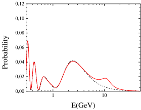
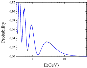
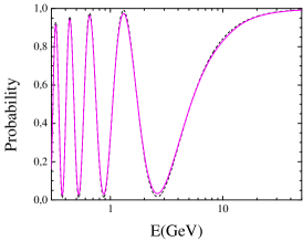
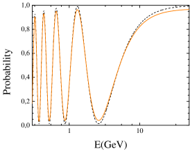
As we can see in Fig. 1, the decoherence parameters affect the four oscillation channels, and for the values of the decoherence parameters considered we can see a few different effects on the oscillation probabilities. In Figs. 1 (c) and (d) there is a small decrease in the overall oscillation amplitude (more accentuated for the $\bar{\nu}_{\mu}$ disappearance probability). In Fig. 1 (d) we can also see a decrease in the $\bar{\nu}_{\mu}$ for $E\gtrsim 10$ GeV. However, the most striking difference respect to the standard oscillation is the new peak at $\sim 10$ GeV for the $\nu_{e}$ appearance probability in the presence of decoherence, which would provide a clear signature of new physics. In the next section we will discuss this feature in more details. Although the peak by itself is not a novelty, and it was somehow studied in previous works (see for instance Oliveira (2016); Coelho and Mann (2017)), here we provide a detailed physical interpretation, and more importantly, we suggest how this unique feature of decoherence can be probed at DUNE.

III.1 New peak at the $\nu_{e}$ appearance probability: physical interpretation

A peak at $\sim 10$ GeV is present in the $\nu_{e}$ appearance probability in the presence of decoherence. In order to obtain a physical insight of this new feature, let us begin by analysing the behavior of the eigenvalues of the Hamiltonian ($\lambda$) in Eq. (9), which can be seen in Fig. 2.

Figure 2: Eigenvalues ($\lambda_{i}$, i=1,2,3) of the Hamiltonian in Eq. (9). We can see an indication of a resonance region about $E\sim 10$ GeV.

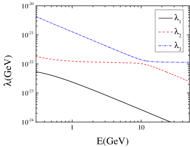
As we can see in Fig. 2, there is a level crossing between the eigenvalues referred as 2 and 3 at $E\sim 10$ GeV, which indicates a resonance at that energy for the parameters considered.

From the oscillation probabilities with decoherence in Eq. (17), the $\Gamma_{jk}$ parameters appear in the form of $e^{-\Gamma_{jk}x}$ damping factors for the terms:

$$\begin{split}I_{\alpha\alpha^{\prime}}=&2\sum_{j>k}Re(\tilde{U}_{\alpha^{\prime}j}\tilde{U}_{\alpha j}^{\ast}\tilde{U}_{\alpha k}\tilde{U}_{\alpha^{\prime}k}^{\ast})\cos\left(\frac{\tilde{\Delta}_{jk}}{2E}x\right)\\ &+2\sum_{j>k}Im(\tilde{U}_{\alpha^{\prime}j}\tilde{U}_{\alpha j}^{\ast}\tilde{U}_{\alpha k}\tilde{U}_{\alpha^{\prime}k}^{\ast})\sin\left(\frac{\tilde{\Delta}_{jk}}{2E}x\right),\end{split}$$ (18)

for $j,k=1,2,3$ and $j>k$.

Since $I_{\alpha\alpha^{\prime}}$ is the term of the probability where we have the dependence on the oscillation phase through $\cos\left(\frac{\tilde{\Delta}_{jk}}{2E}x\right)$ and $\sin\left(\frac{\tilde{\Delta}_{jk}}{2E}x\right)$, which are responsible for the quantum interference in the oscillation probabilities, we will refer to it as the interference factor. In addition, there are terms not affected by the decoherence parameters:

$$C_{\alpha\alpha^{\prime}}=\delta_{\alpha\alpha^{\prime}}-2\sum_{j>k}Re(\tilde{U}_{\alpha^{\prime}j}\tilde{U}_{\alpha j}^{\ast}\tilde{U}_{\alpha k}\tilde{U}_{\alpha^{\prime}k}^{\ast}),$$ (19)

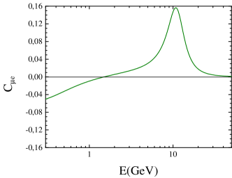
where $j,k=1,2,3$ and $j>k$. The term $C_{\alpha\alpha^{\prime}}$ in the case of the $\nu_{e}$ appearance probability, and for $j=3$ and $k=2$, is given by:

$$C_{\mu e}=-2~{}Re(\tilde{U}_{e3}\tilde{U}_{\mu 3}^{\ast}\tilde{U}_{\mu 2}\tilde{U}_{e2}^{\ast}),$$ (20)

is also shown in the left panel of Fig. 3. This term of the $\nu_{e}$ appearance probability indeed presents a resonance at $E\sim 10$ GeV, which was already suggested by the level crossing in the eigenvalues for this energy in Fig. 2.

Let us now analyse the effect of $e^{-\Gamma_{32}x}$ over the $\nu_{e}$ appearance probability, and in order to do so, we considered the form of the interference factor in Eq. (18) when $j=3$, $k=2$, $\alpha=\mu$, $\alpha^{\prime}=e$:

$$\begin{split}I_{\mu e}=&~{}2~{}Re(\tilde{U}_{e3}\tilde{U}_{\mu 3}^{\ast}\tilde{U}_{\mu 2}\tilde{U}_{e2}^{\ast})\cos\left(\frac{\tilde{\Delta}_{32}}{2E}x\right)\\ &+2~{}Im(\tilde{U}_{e3}\tilde{U}_{\mu 3}^{\ast}\tilde{U}_{\mu 2}\tilde{U}_{e2}^{\ast})\sin\left(\frac{\tilde{\Delta}_{32}}{2E}x\right).\end{split}$$ (21)

Figure 3: Left panel: behavior of $C_{\mu e}$ for $j=3$, $k=2$, $\alpha=\mu$, $\alpha^{\prime}=e$ given by Eq. (20). Right panel: interference factor $I_{\mu e}$ for $j=3$, $k=2$, $\alpha=\mu$, $\alpha^{\prime}=e$ given by Eq. (21).

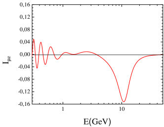
The form of the interference term, which is subject to the damping factor $e^{-\Gamma_{32}x}$, and as given in Eq. (21), is shown in the right panel of Fig. 3. We can see that the term $I_{\mu e}$ work as an interference factor to the oscillation probabilities, in particular, we see that around $E=10.8$ GeV, which is exactly the energy of the resonance, we have a strong destructive interference. For the standard oscillation probabilities (without decoherence), such destructive interference would exactly cancel out the resonance at $E\sim 10.8$ Gev shown in the left panel. In fact, considering a constant matter density of $2.96g/cm^{3}$ Dziewonski and Anderson (1981); Stacey (1969), numerically the maximum of $C_{\mu e}$ in Eq. (20) is equal to the minimum of $I_{\mu e}$ in Eq. (21), and both coincide at $E=10.82$ GeV. However, when we have oscillations with decoherence the term $e^{-\Gamma_{32}x}$ work as a damping to this interference factor, therefore eliminating the destructive interference at $E\sim 10$ GeV. The elimination of such destructive interference enhances the $\nu_{e}$ appearance probability, since now the destructive interference cannot completely cancel out the resonance, therefore creating the peak shown in Fig. 1 (a). Since such peak constitutes a very significant effect in the oscillation probabilities in the presence of decoherence, being able to reconstruct it will provide a compelling test of decoherence. If DUNE is compatible with standard oscillations, severe bounds to the decoherence parameters can be obtained as long as the experiment measure a significant number of events around $E\sim 10$ GeV.

IV Results

In this section we are going to show sensitivity analyses considering neutrino oscillations with decoherence in matter given by Eq. (17). We first show how each oscillation channel is sensible to decoherence by calculating the event rates, and then we establish DUNE sensitivities to the decoherence parameters. For the sensitivity analysis we have considered two neutrino flux configurations, as will be detailed in the following sections, to exploit the main features of the decoherence effects discussed previously.

In the following studies, we assume the DUNE configuration as defined in the CDR document in Ref. Acciarri et al. (2015) and in particular we made use of the GLoBES files from Ref. Alion et al. (2016). Basically, it is assumed DUNE will be running for $3.5$ years in each mode (neutrino and antineutrino), a fiducial mass of the far detector (liquid Argon) of $40\,\text{kt}$, and the default flux beam power of $1.07\,\text{MW}$. The channels considered in each analysis are defined for each case. The systematical errors, energy resolution, and efficiencies are fixed to the values in the CDR studies.

IV.1 Relative events with the DUNE default flux configuration

For a particular input for the decoherence parameters, the total number of events and the energy event spectra are calculated for each oscillation channel. We define the relative Event Rates as $\delta R_{rel}$:

$$\delta R_{rel}=\frac{R(\Gamma_{ij}\neq 0)-R(\Gamma_{21}=\Gamma_{31}=\Gamma_{32}=0)}{R(\Gamma_{21}=\Gamma_{31}=\Gamma_{32}=0)},$$ (22)

where$\Gamma_{ij}\neq 0$ (i.e.: $\Gamma_{21}\neq 0,\Gamma_{31}\neq 0,\Gamma_{32}\neq 0$) are chosen in order to satisfy Eqs. (5) – (7), and $R$ correspond to the event rates.

Figure 4: Relative event rates defined in Eq. (22) setting $\Gamma_{21}=5.1\times 10^{-25}$ GeV, and $\Gamma_{32}=8.9\times 10^{-24}$ GeV, for the event rates in the presence of decoherence.

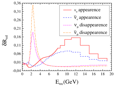
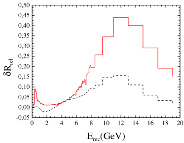
Fig. 4 show the relative deviation of the number of $\nu_{e}$, $\bar{\nu}_{e}$, $\nu_{\mu}$, and $\bar{\nu}_{\mu}$ events in respect to the standard oscillation case without decoherence. From the $\nu_{e}$ and $\bar{\nu}_{e}$ events, one can see a low relative deviation ($<3\%$) at the DUNE flux (default) maximum ($\sim 2.5\,\text{GeV}$). The peak at $E\gtrsim 10$ GeV in the $\nu_{e}$ ($\bar{\nu}_{e}$) events is also relatively low, being about $\sim 16\%$ ($\sim 8\%$), but this is expected because with the default flux events at the high energy end of the spectrum are much smaller than in the DUNE energy peak. In the case of $\nu_{\mu}$ and $\bar{\nu}_{\mu}$ events in Fig. 4 we can notice that at slightly lower energies from the DUNE flux (default) maximum, a relative deviation of the order of $\sim 19\%$ is obtained in the case of $\nu_{\mu}$ and $\sim 35\%$ for $\bar{\nu}_{\mu}$ events.

It appears to be that, with the default flux configuration, DUNE is sensitive to decoherence, and this sensitivity is obtained from the four oscillation channels. However, due to the large number of muon neutrino (and antineutrino) events (see Tab. 2), and the relative deviation in Fig. 4, the main sensitivity comes from $\nu_{\mu}$ and $\bar{\nu}_{\mu}$ events and some reduced sensitivity from $\bar{\nu}_{e}$ events. To fully exploit the high energy relative deviations that appears in the $\nu_{e}$ and $\bar{\nu}_{e}$ events in Fig. 4, a high energy flux for DUNE will be considered in the sensitivity analysis of Section IV.3, and as will be shown, this will substantially improve the sensitivity for testing decoherence.

$\nu_{e}$-app	$\bar{\nu}_{e}$-app	$\nu_{\mu}$-disapp	$\bar{\nu}_{\mu}$-disapp
1777.69	406.025	8206.77	4124.51

Table 2: Total number of events (signal plus background) for each oscillation channel.

IV.2 DUNE sensitivity to the decoherence parameters with the default flux configuration

In this section we present a sensitivity analysis considering the default flux configuration from Alion et al. (2016). From the previous sections we could see that with the default flux DUNE have a good sensitivity to the decoherence parameters $\Gamma_{21}$ and $\Gamma_{32}$ in a parameter range which is not yet constrained by other experiments. Later, we present a second analysis considering a higher energy flux, which will bring a better sensitivity to $\Gamma_{32}$, since it is the parameter which generates the new peak at $\sim 10$ GeV for the $\nu_{e}$ appearance probability.

For the analysis presented in this section we have assumed standard oscillation ‘data’ without decoherence using values in Table 1 and tested the decoherence hypothesis. The usual $\chi^{2}$ analysis have been performed marginalizing over the standard oscillation parameters (except the solar parameters that are kept fixed) adding penalties to the $\chi^{2}$-function with the following standard deviations: $\sigma(\sin^{2}{(2\theta_{13})})=0.0033$, $\sigma(\sin^{2}{(2\theta_{23})})/\sin^{2}{(2\theta_{23})}=3\%$, and $\sigma(\Delta m^{2}_{31})/\Delta m^{2}_{31}=3\%$. The $\delta$ parameter have been also minimized over.

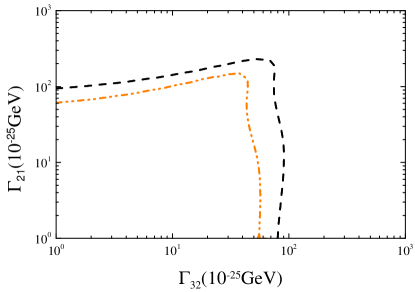
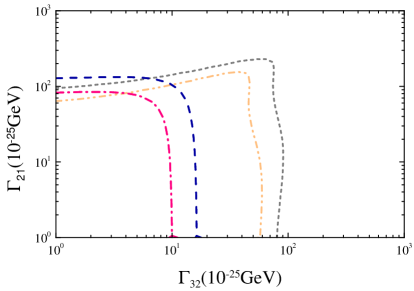
Because $\Gamma_{21},\Gamma_{31},\Gamma_{32}$ are not all independent, to perform the $\chi^{2}$ analysis we assumed two of the three decoherence parameters as independent, and defined the other one as a dependent parameter, according to Eqs. (5), Eq. (6) and Eq. (7), making then confidence level curves shown in Fig. 5.

Figure 5: Confidence Level curves at $90\%$ C.L and $3\sigma$ C.L for $2$ d.of.. for the two decoherence parameters $\Gamma_{21}$ and $\Gamma_{32}$, considering the Default Flux given by Alion et al. (2016).

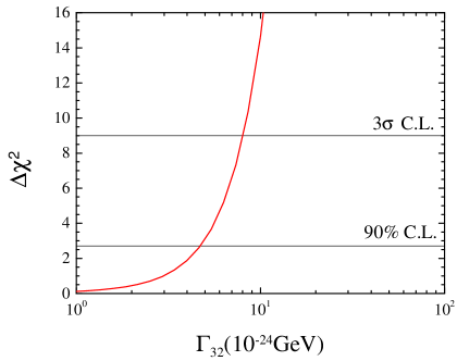
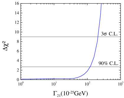
To obtain the sensitivity regions on each individual parameter we perform the minimization over each of the two decoherence parameters as shown in Fig. 6 (a) for $\Delta\chi^{2}$ versus $\Gamma_{32}$ and (b) for $\Delta\chi^{2}$ versus $\Gamma_{21}$. From the $\Delta\chi^{2}$ profiles we obtained sensitivity regions compiled in table 3. From the results in table 3 we can see that DUNE has the potential to provide a more stringent limit to $\Gamma_{21}$ than the one given by KamLAND in Ref. Balieiro Gomes et al. (2017), where the limit for $\Gamma_{21}$ in $95\%$ C.L. is $6.8\times 10^{-22}$ GeV.

(a) $\Delta\chi^{2}$ versus $\Gamma_{32}$, minimizing over $\Gamma_{21}$

(b) $\Delta\chi^{2}$ versus $\Gamma_{21}$, minimizing over $\Gamma_{32}$

Figure 6: Sensitivity analysis for the Default Flux given by Alion et al. (2016). The horizontal lines define $90\%$ C.L. and $3\sigma$ C.L.

Parameter	$90\%$ C.L	$3\sigma$ C.L
$\Gamma_{21}\leq$	$1.2\times 10^{-23}\,\text{GeV}$	$2.1\times 10^{-23}\,\text{GeV}$
$\Gamma_{32}\leq$	$4.7\times 10^{-24}\,\text{GeV}$	$8.0\times 10^{-24}\,\text{GeV}$

Table 3: Sensitivity regions for the decoherence parameters from the $\chi^{2}$ analysis considering the default flux configuration Alion et al. (2016), as shown in Fig. 6 (a) and 6 (b) for 1 d.o.f.

In the following section we discuss how a high energy neutrino flux, different from the one given by Ref. Alion et al. (2016), can considerably improve the sensitivity to $\Gamma_{32}$ providing a more suitable configuration to test decoherence at DUNE.

IV.3 Sensitivity analysis for $\Gamma_{32}$ with a high energy flux configuration

From the discussion at the event level in Section IV.1 it is clear that in order to be sensitive to the peak around $10$ GeV in the $\nu_{e}$ appearance channel at DUNE, it is necessary to consider a different flux configuration. Having reached this conclusion, we decided to perform a second sensitivity analysis, but this time considering the High Energy (HE) neutrino flux proposed in Ref. Masud et al. (2017).

For the sensitivity analysis using the HE flux we excluded the beam contamination from $\nu_{e}$ and $\overline{\nu}_{e}$, since we do not have access to this information. Then, we repeated the same procedure of the previous sections, first presenting in Fig. 7 the relative deviation of the number of $\nu_{e}$ events respect to the standard oscillation case without decoherence and finally the sensitivity results. As already expected, with the HE flux configuration the peak at in the $\nu_{e}$ rises to $\sim 45\%$, which suggests that this channel with such flux configuration can bring increased sensitivity to the $\Gamma_{32}$ parameter. We showed in Section III, that is the $\Gamma_{32}$ parameter that mostly generates this new peak. Following the same procedure of the previous section we performed another sensitivity analysis, and the results are given in Fig. 8 and Fig. 9.

Figure 7: Relative deviations respect to the $\nu_{e}$ appearance events without decoherence ($\Gamma_{32}=0$) for the HE flux from Masud et al. (2017). For the event rates with decoherence we considered $\Gamma_{21}=5.1\times 10^{-25}$ GeV, $\Gamma_{31}=3.0\times 10^{-25}$ GeV, $\Gamma_{32}=1.6\times 10^{-24}$ GeV. We also present again the Relative deviations for the $\nu_{e}$ appearance events considering the default flux Alion et al. (2016) for comparison.

Figure 8: $\Gamma_{32}$ versus $\Gamma_{21}$ Confidence Level curves for $90\%$ C.L and $3\sigma$ C.L. considering the HE Flux given by Masud et al. (2017). The Confidence Level curves for the Default Flux Alion et al. (2016) are also shown for comparison.

Figure 9: $\Delta\chi^{2}$ versus $\Gamma_{32}$, minimizing over $\Gamma_{21}$, comparing the results between the Default Flux Alion et al. (2016) and the HE flux Masud et al. (2017). The horizontal lines define $90\%$ C.L. and $3\sigma$ C.L.

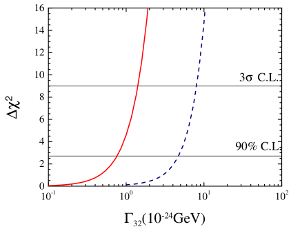
From Fig. 9 we obtained the sensitivity regions compiled in Table 4, where we present only the limits for $\Gamma_{32}$, since the analysis presented in section IV.2 already brings the best sensitivity to $\Gamma_{21}$. Sensitivity to $\Gamma_{32}$ given in Table 4 is enhanced respect to the one found in Section IV.2, since the HE flux from Masud et al. (2017) is much more suitable to pin down the new peak at $E\sim 10.8$ GeV in the $\nu_{e}$ appearance probability than the default flux Alion et al. (2016). DUNE has the potential to put a stringent limit to the decoherence parameters, which means that the peak would become much less noticeable in a $\nu_{e}$ appearance probability plot as long as the DUNE measured rates are more ‘compatible’ with standard oscillations.

Parameter	$90\%$ C.L	$3\sigma$ C.L
$\Gamma_{32}\leq$	$7.7\times 10^{-25}\,\text{GeV}$	$1.4\times 10^{-24}\,\text{GeV}$

Table 4: Sensitivities to the decoherence parameters from the $\chi^{2}$ analysis considering the HE flux configuration Masud et al. (2017) shown in Fig. 9 for 1 d.o.f.

V Conclusion

In this work we found sensitivity regions for the decoherence parameters that affect neutrino oscillations in three families considering two possible flux configurations for DUNE.

In Section III we showed how the new peak at the $\nu_{e}$ appearance probability can be seen as an elimination of a destructive interference, generating then an increase in the transition to $\nu_{e}$. In Section IV we showed how the decoherence parameters can be better analyzed by considering different oscillation channels and also different flux configurations, the default flux from Alion et al. (2016) and the HE flux from Masud et al. (2017).

In Section IV.2 we presented the results for the sensitivity analysis using the flux configuration from Ref. Alion et al. (2016). In $90\%$ C. L. the sensitivity limits for the parameters given in Table 3 are: $\Gamma_{21}\leq 1.2\times 10^{-23}\,\text{GeV}$ and $\Gamma_{32}\leq 4.7\times 10^{-24}\,\text{GeV}$, and for $3\sigma$ C.L. the limits are: $\Gamma_{21}\leq 2.1\times 10^{-23}\,\text{GeV}$and $\Gamma_{32}\leq 8.0\times 10^{-24}\,\text{GeV}$.

As we can see, the limits on $\Gamma_{21}$ are potentially more stringent at DUNE, when compared with the KamLAND experiment, by two orders of magnitude. On the other hand, DUNE in its default configuration has a reduced sensitivity for $\bar{\nu}_{e}$, suggesting that the limit for $\Gamma_{21}$ comes in most part from the $\nu_{e}$ channel. Therefore, one might think that $\Gamma_{21}$ for $\nu_{e}$ and $\bar{\nu}_{e}$ has some chance to be different. This is the exact scenario for a CPT-like violation such as was proposed in Ref Barenboim and Mavromatos (2005) and a new investigation regarding such issue will be presented somewhere else.

Finally, in Section IV.3 we showed how changing to a HE flux configuration DUNE can significantly improve the sensitivity to the $\Gamma_{32}$ parameter potentially pinning down the peak which is the most compelling feature of decoherence at DUNE. The sensitivity regions for such analysis (presented in Table 4) are, for $90\%$ C.L.: $\Gamma_{32}\leq 7.7\times 10^{-25}\,\text{GeV}$, and for $3\sigma$ C.L. $\Gamma_{32}\leq 1.4\times 10^{-24}\,\text{GeV}$.

Appendix A Conditions on $D_{\mu\nu}$

The Lindblad equation that describes the open system’s dynamics is given by:

$$\frac{d\rho(t)}{dt}=-i[H,\rho(t)]+\frac{1}{2}\sum_{j=1}^{8}\left(\left[V_{j},\rho(t)V_{j}^{\dagger}\right]+\left[V_{j}\rho(t),V_{j}^{\dagger}\right]\right)$$ (23)

where $V_{j}$ are $3\times 3$ matrices that carry out the new dynamics. Expanding in Gell-Mann matrices in mass eigenbasis, where $H$ is diagonal, we have:

$$H=h_{3}\lambda_{3}+h_{8}\lambda_{8}~{}~{}~{};~{}~{}~{}V_{j}=\sum_{i=1}^{8}v_{ji}\lambda_{i}~{}~{}~{};~{}~{}~{}\rho=\sum_{i=1}^{8}\rho_{i}\lambda_{i}$$

where, since $V_{j}$ is hermitian, all coeficients are real. The energy conservation condition, $[V_{j},H]=0$, leads to:

$$[V_{j},H] = \sum_{i}\left(h_{3}v_{ji}[\lambda_{i},\lambda_{3}]+h_{8}v_{ji}[\lambda_{i},\lambda_{8}]\right)$$

$$= 2i\sum_{i,k}v_{ji}\left(h_{3}f_{i3k}+h_{8}f_{i8k}\right)\lambda_{k}=0$$

The only way to accomplish this with no dependence on $h_{3,8}$ is that all $v_{ji}$ vanishes except for $v_{j3}$ and $v_{j8}$. Then:

$$V_{j}=v_{j3}\lambda_{3}+v_{j8}\lambda_{8}$$

By replacing in the Lindblad equation we obtain:

$$\frac{d\rho_{k}(t)}{dt}\lambda_{k} = 2h_{m}\rho_{n}f_{mnk}\lambda_{k}+\frac{1}{2}\sum_{j=1}^{8}\sum_{k=1}^{8}\sum_{l=3,8}\sum_{m=3,8}\rho_{k}v_{jl}v_{jm}^{*}\left([\lambda_{l},\lambda_{k}\lambda_{m}^{\dagger}]+[\lambda_{l}\lambda_{k},\lambda_{m}^{\dagger}]\right)$$

$$= 2h_{m}\rho_{n}f_{mnk}\lambda_{k}+\frac{1}{2}\left(\sum_{j}|v_{j3}|^{2}\right)\sum_{k}\rho_{k}\left(\left[\lambda_{3},\lambda_{k}\lambda_{3}^{\dagger}\right]+\left[\lambda_{3}\lambda_{k},\lambda_{3}^{\dagger}\right]\right)$$

$$+ \frac{1}{2}\left(\sum_{j}|v_{j8}|^{2}\right)\sum_{k}\rho_{k}\left(\left[\lambda_{8},\lambda_{k}\lambda_{8}^{\dagger}\right]+\left[\lambda_{8}\lambda_{k},\lambda_{8}^{\dagger}\right]\right)$$

$$+ \frac{1}{2}\left(\sum_{j}v_{j3}v_{j8}^{*}\right)\sum_{k}\rho_{k}\left(\left[\lambda_{3},\lambda_{k}\lambda_{8}^{\dagger}\right]+\left[\lambda_{3}\lambda_{k},\lambda_{8}^{\dagger}\right]\right)$$

$$+ \frac{1}{2}\left(\sum_{j}v_{j3}^{*}v_{j8}\right)\sum_{k}\rho_{k}\left(\left[\lambda_{8},\lambda_{k}\lambda_{3}^{\dagger}\right]+\left[\lambda_{8}\lambda_{k},\lambda_{3}^{\dagger}\right]\right)$$

Performing the last sum by direct inspection we get:

$$I_{1} = [\lambda_{3},\lambda_{k}\lambda_{3}]+[\lambda_{3}\lambda_{k},\lambda_{3}]$$

$$= \lambda_{3}[\lambda_{k},\lambda_{3}]+[\lambda_{3},\lambda_{k}]\lambda_{3}$$

$$= 2i(\lambda_{3}\sum_{l}f_{k3l}\lambda_{l}+\sum_{l}f_{3kl}\lambda_{l}\lambda_{3})$$

$$= 2i\sum_{l}f_{3kl}[\lambda_{l},\lambda_{3}]=-4\sum_{lm}f_{3kl}f_{l3m}\lambda_{m}=-4\lambda_{k}\sum_{l}(f_{3kl})^{2}$$

$$\sum_{k}\rho_{k}I_{1}=-(4,4,0,1,1,1,1,0).(\rho_{k}\lambda_{k})$$

and with a similar procedure:

$$I_{2} = [\lambda_{8},\lambda_{k}\lambda_{8}]+[\lambda_{8}\lambda_{k},\lambda_{8}]=-4\lambda_{k}\sum_{l}(f_{8kl})^{2}$$

$$\sum_{k}\rho_{k}I_{k}=-3(0,0,0,1,1,1,1,0).(\rho_{k}\lambda_{k})$$

The last two lines can be simplified since $v_{ij}$ are real numbers. In this case the last two lines can be summed up:

$$I_{3} = {\rm[}\lambda_{3},\lambda_{k}\lambda_{8}{\rm]}+{\rm[}\lambda_{3}\lambda_{k},\lambda_{8}{\rm]}+(3\leftrightarrow 8)=-8\lambda_{k}\sum_{l}f_{8kl}f_{3kl}$$

$$\sum_{k}\rho_{k}I_{3}=-2\sqrt{3}(0,0,0,1,1,-1,-1,0).(\lambda_{k}\rho_{k})$$

Defining the 8-dimensional vectors $\vec{a}_{k}$ formed by the components $v_{jk}$ in the following way:

$$(\vec{a}_{3})_{j}\equiv v_{j3}~{}~{}~{};~{}~{}~{}(\vec{a}_{8})_{j}\equiv\sqrt{3}v_{j8}$$

we have:

$$\sum_{j}|v_{j3}|^{2}=a_{3}^{2}~{}~{}~{};~{}~{}~{}\sum_{j}|v_{j8}|^{2}=\frac{a_{8}^{2}}{3}~{}~{}~{};~{}~{}~{}\sum_{j}(v_{j3}v_{j8}^{*})=\frac{1}{\sqrt{3}}(\vec{a}_{3}^{\,\dagger}.\vec{a}_{8})$$

we can finally write:

$$\frac{d\rho(t)}{dt} = -i[H,\rho(t)]+\frac{1}{2}\left(a_{3}^{2}I_{1}+a_{8}^{2}\frac{I_{2}}{3}+2\vec{a}_{3}^{\,\dagger}.\vec{a}_{8}\frac{I_{3}}{2\sqrt{3}}\right)$$

and

$$D_{mn}=-\frac{1}{2}{\rm diag}(4a_{3}^{2},4a_{3}^{2},0,(\vec{a}_{3}+\vec{a}_{8})^{2},(\vec{a}_{3}+\vec{a}_{8})^{2},(\vec{a}_{3}-\vec{a}_{8})^{2},(\vec{a}_{3}-\vec{a}_{8})^{2},0)$$

or

$$D_{mn}=-{\rm diag}(\Gamma_{21},\Gamma_{21},0,\Gamma_{31},\Gamma_{31},\Gamma_{32},\Gamma_{32},0)$$

where

$$\Gamma_{21}\equiv 2a_{3}^{2}~{}~{}~{};~{}~{}~{}\Gamma_{31}\equiv\frac{1}{2}(\vec{a}_{3}+\vec{a}_{8})^{2}~{}~{}~{};~{}~{}~{}\Gamma_{32}\equiv\frac{1}{2}(\vec{a}_{3}-\vec{a}_{8})^{2}$$

For simplicity we treated $\vec{a}_{3}$ and $\vec{a}_{8}$ as colinear, so they were treated as scalars. So the conclusion is that the matrix energy conservation in the neutrino sector requires a diagonal format for $D_{mn}$, with a specific relation between its terms.

Appendix B Decoherence in matter and positivity

The authors of Ref. Carpio et al. (2018) claim that decoherence cannot be defined in the effective mass basis, and that (apart from very specific cases) the forms of the dissipative matrices in vacuum and in matter cannot be the same. In this appendix we comment that, under certain conditions, decoherence can be defined as arising from the same matrices in both contexts, such that it preserves a physical interpretation where the decoherence effect acts only on the quantum interference terms, such as was discussed in this paper and also in Refs. Balieiro Gomes et al. (2017); Guzzo et al. (2016).

The dissipator in Eq. (4) is obtained when it is imposed that

$$[H_{S},V_{k}]=0,$$ (24)

where $H_{S}$ is the Hamiltonian of the subsystem.

Since the subsystem is different when one considers neutrinos in vacuum or in matter, if $V_{k}$ has the same form in both bases, then Eq. 24 is not satisfied at the same time in such cases. This is exactly what happens in Refs. Fogli et al. (2007); Carpio et al. (2018). As it is shown in Guzzo et al. (2016), this implies that the decoherence effect and the so called relaxation effect cannot be fully separated. In fact, as argued in Refs. Balieiro Gomes et al. (2017); Guzzo et al. (2016), the work in Fogli et al. (2007) finds constraints for the relaxation effect, or for decoherence in a model dependent approach. It is important to point out that decoherence is an effect which acts only on the quantum interference terms of the oscillation probabilities, while relaxation acts only on the constant terms, which allow flavor conversion even without mixing between the neutrino families.

For two neutrino families Guzzo et al. (2016) we have that the parameterization:

$$\tilde{V}_{k}=\sqrt{\gamma_{1}}\left(\begin{array}[]{cc}\cos\delta_{\theta}&-\sin\delta_{\theta}\\ -\sin\delta_{\theta}&-\cos\delta_{\theta}\end{array}\right),$$ (25)

with $\delta_{\theta}=2(\tilde{\theta}-\theta)$, such that $\tilde{\theta}$ is the effective mixing angle in matter, leaves eq.(24) unchanged for any matter density.

As we can see, in vacuum Eq. (25) assumes the following form:

$$V_{k}=\sqrt{\gamma_{1}}\left(\begin{array}[]{cc}1&0\\ 0&-1\end{array}\right),$$ (26)

since in vacuum $\delta_{\theta}=0$.

To assure that the condition Eq. (24) is satisfied for neutrinos propagating in both vacuum and in constant density matter, it is shown in Ref. Guzzo et al. (2016) that the operators $V_{k}$ must also transform when there is a change of basis. Therefore we must have that:

$$\tilde{V}_{k}=U_{T}^{\dagger}V_{k}U_{T}=\sqrt{\gamma_{1}}\left(\begin{array}[]{cc}1&0\\ 0&-1\end{array}\right),$$ (27)

where $U_{T}=U^{\dagger}U_{M}$, and $U_{M}$ is the rotation matrix between the flavor basis and the effective mass basis, and as we can see, it is equal to Eq. (26).

When $V_{k}$ transform as Eq. (27) the dissipator in Eq. (4) (where we only consider decoherence, not relaxation) is valid for neutrinos propagating in both vacuum and in matter. Since the form is the same, the conditions for positivity are also the same for both cases, which assures that when Eqs. (5) – (7) are obeyed the physical meaning of the probabilities are guaranteed for oscillation both in vacuum and in matter. It is also important to point out that, different from what is assumed by Ref. Carpio et al. (2018), in this work decoherence is assumed to be dependent on the matter density, as can be seen from Eq. (25). More details of this discussion can be found in Ref. Guzzo et al. (2016) for the case of two neutrinos.

It is worth to notice that, even though the calculations presented in Ref. Guzzo et al. (2016) were made for the case of two neutrinos, the discussion of the concepts involved is very general, and its conclusions can be extended to the three neutrino case.

References

- de Salas et al. (2017) P. F. de Salas, D. V. Forero, C. A. Ternes, M. Tortola, and J. W. F. Valle, (2017), arXiv:1708.01186 [hep-ph] .
- Acciarri et al. (2016a) R. Acciarri et al. (DUNE), (2016a), arXiv:1601.05471 [physics.ins-det] .
- Acciarri et al. (2015) R. Acciarri et al. (DUNE), (2015), arXiv:1512.06148 [physics.ins-det] .
- Strait et al. (2016) J. Strait et al. (DUNE), (2016), arXiv:1601.05823 [physics.ins-det] .
- Acciarri et al. (2016b) R. Acciarri et al. (DUNE), (2016b), arXiv:1601.02984 [physics.ins-det] .
- (6) LBNF/DUNE, “Long-Baseline Neutrino Facility (LBNF) and Deep Underground Neutrino Experiment (DUNE) : Conceptual Design Report, Volume 3, Annex 3 A: Beamline at the Near Site,” .
- Oliveira and Guzzo (2013) R. L. N. Oliveira and M. M. Guzzo, Eur. Phys. J. C73, 2434 (2013).
- Guzzo et al. (2016) M. M. Guzzo, P. C. de Holanda, and R. L. N. Oliveira, Nucl. Phys. B908, 408 (2016), arXiv:1408.0823 [hep-ph] .
- Balieiro Gomes et al. (2017) G. Balieiro Gomes, M. M. Guzzo, P. C. de Holanda, and R. L. N. Oliveira, Phys. Rev. D95, 113005 (2017), arXiv:1603.04126 [hep-ph] .
- Fogli et al. (2007) G. L. Fogli, E. Lisi, A. Marrone, D. Montanino, and A. Palazzo, Phys. Rev. D76, 033006 (2007), arXiv:0704.2568 [hep-ph] .
- Oliveira and Guzzo (2010) R. L. N. Oliveira and M. M. Guzzo, Eur. Phys. J. C69, 493 (2010).
- Coelho et al. (2017) J. A. B. Coelho, W. A. Mann, and S. S. Bashar, Phys. Rev. Lett. 118, 221801 (2017), arXiv:1702.04738 [hep-ph] .
- Oliveira (2016) R. L. N. Oliveira, Eur. Phys. J. C76, 417 (2016), arXiv:1603.08065 [hep-ph] .
- Coelho and Mann (2017) J. A. B. Coelho and W. A. Mann, Phys. Rev. D96, 093009 (2017), arXiv:1708.05495 [hep-ph] .
- de Oliveira et al. (2014) R. L. N. de Oliveira, M. M. Guzzo, and P. C. de Holanda, Phys. Rev. D89, 053002 (2014), arXiv:1401.0033 [hep-ph] .
- Carpio et al. (2018) J. A. Carpio, E. Massoni, and A. M. Gago, Phys. Rev. D97, 115017 (2018), arXiv:1711.03680 [hep-ph] .
- Coloma et al. (2018) P. Coloma, J. Lopez-Pavon, I. Martinez-Soler, and H. Nunokawa, (2018), arXiv:1803.04438 [hep-ph] .
- Breuer and Petruccione (2002) H. P. Breuer and F. Petruccione, The theory of open quantum systems (2002).
- Ellis et al. (1984) J. R. Ellis, J. S. Hagelin, D. V. Nanopoulos, and M. Srednicki, Proceedings: LAMPF II Workshop, 3rd, Los Alamos, N.Mex., Jul 18-28, 1983, Nucl. Phys. B241, 381 (1984), [,580(1983)].
- Akhmedov et al. (2017) E. Akhmedov, J. Kopp, and M. Lindner, JCAP 1709, 017 (2017), arXiv:1702.08338 [hep-ph] .
- An et al. (2017a) F. P. An et al. (Daya Bay), Eur. Phys. J. C77, 606 (2017a), arXiv:1608.01661 [hep-ex] .
- Cohen-Tannoudji et al. (1977) C. Cohen-Tannoudji, B. Diu, and F. Laloë, Quantum mechanics (Wiley, 1977).
- Barenboim and Mavromatos (2005) G. Barenboim and N. E. Mavromatos, JHEP 01, 034 (2005), arXiv:hep-ph/0404014 [hep-ph] .
- Huber et al. (2005) P. Huber, M. Lindner, and W. Winter, Comput. Phys. Commun. 167, 195 (2005), arXiv:hep-ph/0407333 [hep-ph] .
- Huber et al. (2007) P. Huber, J. Kopp, M. Lindner, M. Rolinec, and W. Winter, Comput. Phys. Commun. 177, 432 (2007), arXiv:hep-ph/0701187 [hep-ph] .
- An et al. (2017b) F. P. An et al. (Daya Bay), Phys. Rev. D95, 072006 (2017b), arXiv:1610.04802 [hep-ex] .
- Abe et al. (2017) K. Abe et al. (T2K), Phys. Rev. D96, 092006 (2017), arXiv:1707.01048 [hep-ex] .
- Dziewonski and Anderson (1981) A. M. Dziewonski and D. L. Anderson, Phys. Earth Planet. Interiors 25, 297 (1981).
- Stacey (1969) F. Stacey, Physics of the earth (Wiley, 1969).
- Alion et al. (2016) T. Alion et al. (DUNE), (2016), arXiv:1606.09550 [physics.ins-det] .
- Masud et al. (2017) M. Masud, M. Bishai, and P. Mehta, (2017), arXiv:1704.08650 [hep-ph] .