Log Gaussian Cox Process Networks

Abstract

We generalize the log Gaussian Cox process (lgcp) framework to model multiple correlated point data jointly. The observations are treated as realizations of multiple lgcps, whose log intensities are given by linear combinations of latent functions drawn from Gaussian process priors. The combination coefficients are also drawn from Gaussian processes and can incorporate additional dependencies. We derive closed-form expressions for the moments of the intensity functions and develop an efficient variational inference algorithm that is orders of magnitude faster than competing deterministic and stochastic approximations of multivariate lgcps, coregionalization models, and multi-task permanental processes. Our approach outperforms these benchmarks in multiple problems, offering the current state of the art in modeling multivariate point processes.

 

Efficient Inference in Multi-task Cox Process Models

 

Virginia Aglietti                        Theodoros Damoulas                        Edwin V. Bonilla

University of Warwick The Alan Turing Institute                        University of Warwick The Alan Turing Institute                        CSIRO’s Data61 UNSW

1 Introduction

Many problems in urban science and geostatistics are characterized by count or point data observed in a spatio-temporal region. Crime events, traffic or human population dynamics are some examples. Furthermore, in many settings, these processes can be strongly correlated. For example, in a city such as New York (nyc), burglaries can be highly predictive of other crimes’ occurrences such as robberies and larcenies. These settings are multi-task problems and our goal is to exploit such dependencies in order to improve the generalization capabilities of our learning algorithms.

Typically such settings can be modeled as inhomogeneous processes where a space-time varying underlying intensity determines event occurrences. Among these modeling approaches, the log Gaussian Cox process (lgcp, Møller et al.,, 1998) is one of the most well-established frameworks, where the intensity is driven by a Gaussian process prior (gp, Williams and Rasmussen,, 2006). The flexibility of lgcp comes at the cost of incredibly hard inference challenges due to its doubly-stochastic nature and the notorious scalability issues of gp models. The computational problems are exacerbated when considering multiple correlated tasks and, therefore, the development of new approaches and scalable inference algorithms for lgcp models remains an active area of research (Diggle et al.,, 2013; Flaxman et al.,, 2015; Taylor et al.,, 2015; Leininger et al.,, 2017).

From a modeling perspective, existing multivariate lgcps or linear-coregionalization-model (lcm) variants for point processes have intensities given by deterministic combinations of latent gps (Diggle et al.,, 2013; Taylor et al.,, 2015; Alvarez et al.,, 2012). These approaches fail to propagate uncertainty in the weights of the linear combination, leading to statistical deficiencies that we address. For instance, Fig. 1 shows how, by propagating uncertainty, our approach (mcpm) provides a predictive distribution that contains the counts’ ground truth in its 90% credible interval (ci). This is not observed for the standard intrinsic coregionalization model (icm, see e.g. Alvarez et al.,, 2012).

From an inference point of view, sampling approaches have been proposed (Diggle et al.,, 2013; Taylor et al.,, 2015) and variational inference algorithms for models with gp priors and ‘black-box’ likelihoods have been used (see e.g. Matthews et al.,, 2017; Dezfouli and Bonilla,, 2015). While sampling approaches have prohibitive computational cost (Shirota and Gelfand,, 2016) and mixing issues (Diggle et al.,, 2013), generic methods based on variational inference do not exploit the lgcp likelihood details and, relying upon Monte Carlo estimates for computing expectations during optimization, can exhibit slow convergence.

In this paper we address the modeling and inference limitations of current approaches. More specifically, we make the following contributions.

Stochastic mixing weights: We propose a model that considers correlated count data as realizations of multiple lgcps, where the log intensities are linear combinations of latent gps and the combination coefficients are also gps. This provides additional model flexibility and the ability to propagate uncertainty in a principled way.

Efficient inference: We carry out posterior estimation over both latent and mixing processes using variational inference. Our method is orders of magnitude faster than competing approaches.

Closed-form expectations in the variational objective: We express the required expectations in the variational inference objective (so called evidence lower bound), in terms of moment generating functions (mgfs) of the log intensities, for which we provide analytical expressions. We thus avoid Monte Carlo estimates altogether (which are commonplace in modern variational inference methods).

First existing experimental comparison and state-of-the-art performance: To the best of our knowledge, we are the first to provide an experimental comparison between existing multi-task point process methods. This is important as there are currently two dominant approaches (based on the lgcp or on the permanental process), for which there is little insight on which one performs better. Furthermore, we show that our method provides the best predictive performance on two large-scale multi-task point process problems with very different spatial cross-correlation structures.

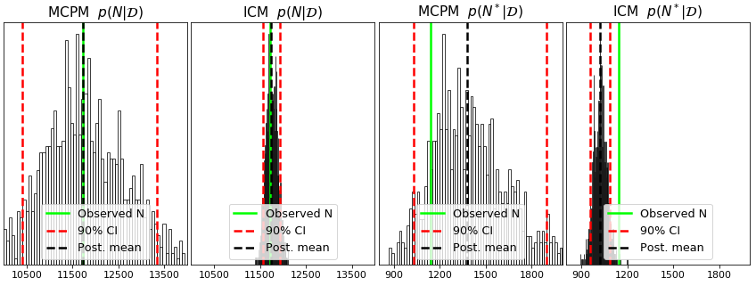
Figure 1: Posterior and predictive distributions, $p(N|\mathcal{D})$ and $p(N^{*}|\mathcal{D})$ respectively, of the number of burglary events in nyc using a similar analysis as in Leininger et al., (2017) on the crime dataset (§5.1) for our model (mcpm) and icm. The solid line shows the ground truth. Details on the ci construction are in §5.

2 The mcpm model

The log Gaussian Cox process (lgcp, Møller et al.,, 1998) is an inhomogeneous Poisson process with a stochastic intensity function (see e.g. Cox,, 1955), where the logarithm of the intensity surface is a gp (Williams and Rasmussen,, 2006). Given an input $\mathbf{x}$, a gp, denoted as $f(\mathbf{x})\sim\mathcal{GP}(m(\mathbf{x}),\kappa(\mathbf{x},\mathbf{x}^{\prime};\boldsymbol{\theta}))$, is completely specified by its mean function $m(\mathbf{x})$ and its covariance function $\kappa(\mathbf{x},\mathbf{x}^{\prime};\boldsymbol{\theta})$ parametrized by the hyper-parameters $\boldsymbol{\theta}$. Conditioned on the realization of the intensity function, the number of points in an area, say $A$, is given by $y_{A}|\lambda(\mathbf{x})\sim\text{Poisson}\left(\int_{\mathbf{x}\in A}\lambda(\mathbf{x})d\mathbf{x}\right)$ with $\lambda(\mathbf{x})=\text{exp}\{f(\mathbf{x})\}$.

2.1 Model formulation

We consider learning problems where we are given a dataset $\mathcal{D}=\{(\mathbf{x}_{n},\mathbf{y}_{n})\}_{n=1}^{N}$ where $\mathbf{x}_{n}\in\mathbb{R}^{D}$ represents the input and $\mathbf{y}_{n}\in\mathbb{R}^{P}$ gives the event counts for the $P$ tasks. We aim at learning the latent intensity functions and make probabilistic predictions of the event counts. Our modelling approach, which we call mcpm, is characterized by $Q$ latent functions which are uncorrelated a priori and are drawn from $Q$ zero-mean gps, i.e. $f_{q}|\boldsymbol{\theta}_{q}\sim\mathcal{GP}(\mathbf{0},\kappa(\mathbf{x},\mathbf{x}^{\prime};\boldsymbol{\theta}_{q}))$, for $q=1,\ldots,Q$. Hence, the prior over all the $N\times Q$ latent function values $\mathbf{F}$ is:

$$p(\mathbf{F}|\boldsymbol{\theta}_{f})=\prod_{q=1}^{Q}p(\mathbf{F}_{\bullet q}|\boldsymbol{\theta}_{f}^{q})=\prod_{q=1}^{Q}\mathcal{N}(\mathbf{F}_{\bullet q};\mathbf{0},\mathbf{K}_{xx}^{q})\text{,}$$ (1)

where $\boldsymbol{\theta}_{q}$ is the set of hyper-parameters for the $q$-th latent function and $\mathbf{F}_{\bullet q}=\{f_{q}(\mathbf{x}_{n})\}_{n=1}^{N}$ denotes the values of latent function $q$ for the observations $\{\mathbf{x}_{n}\}_{n=1}^{N}$. We model tasks’ correlation by linearly combining the above latent functions with a set of stochastic task-specific mixing weights, $\mathbf{W}\in\mathbb{R}^{P\times Q}$, determining the contribution of each latent function to the overall lgcp intensity. We consider two possible prior distributions for $\mathbf{W}$, an independent prior and a correlated prior.

Prior over weights

We assume weights drawn from $Q$ zero-mean gps:

$$p(\mathbf{W}|\boldsymbol{\theta}_{w})=\prod_{q=1}^{Q}p(\mathbf{W}_{\bullet q}|\boldsymbol{\theta}_{w}^{q})=\prod_{q=1}^{Q}\mathcal{N}(\mathbf{W}_{\bullet q};\mathbf{0},\boldsymbol{\mathbf{K}}_{w}^{q})\text{,}$$ (2)

where $\mathbf{W}_{\bullet q}$ represents the $P$ weights for the $q$-th latent function and $\boldsymbol{\theta}_{w}$ denotes the hyper-parameters. In the independent scenario, we assume uncorrelated weights across tasks and latent functions by making $\boldsymbol{\mathbf{K}}_{w}^{q}$ diagonal. The observations across tasks are still correlated via the linear mixing of latent random functions.

Likelihood model

The likelihood of events at locations $\{\mathbf{x}_{n_{p}}\}$ under $P$ independent inhomogeneous Poisson processes each with rate function $\lambda_{p}(\cdot)$ is

$$\exp\left[-\sum_{p=1}^{{P}}\int_{\tau}\lambda_{p}(\mathbf{x})d\mathbf{x}\right]\prod_{p=1}^{P}\prod_{n_{p}=1}^{N_{p}}\lambda_{p}(\mathbf{x}_{n_{p}}),$$

where $\tau$ is the observation domain. Following a common approach we introduce a regular computational grid (Diggle et al.,, 2013) on the spatial extent and represent each cell with its centroid. Under mcpm, the likelihood of the observed counts $\mathbf{Y}=\{\mathbf{y}_{n}\}_{n=1}^{N}$ is defined as:

$$p(\mathbf{Y}|\mathbf{F},\mathbf{W})=\prod_{n=1}^{N}\prod_{p=1}^{P}\text{Poisson}\left(y_{np};\exp\left(\mathbf{W}_{p\bullet}\mathbf{F}_{n\bullet}+\phi_{p}\right)\right)\text{,}$$ (3)

where $y_{np}$ denotes the event counts for the $p$-th task at $\mathbf{x}_{n}$, $\mathbf{W}_{p\bullet}$ represents the $Q$ weights for the $p$-th task, $\mathbf{F}_{n\bullet}$ denotes the $Q$ latent function values corresponding to $\mathbf{x}_{n}$, and $\phi_{p}$ indicates the task-specific offset to the log-mean of the Poisson process.

As in the standard lgcp model, introducing a gp prior poses significant computational challenges during posterior estimation as, naïvely, inference would be dominated by algebraic operations that are cubic in $N$. To make inference scalable, we follow the inducing-variable approach proposed by Titsias, (2009) and further developed by Bonilla et al., (2016). To this end, we augment our prior over the latent functions in Eq. (1) with $M$ underlying inducing variables for each latent process. We denote these $M$ inducing variables for latent process $q$ with $\mathbf{U}_{\bullet q}$ and their corresponding inducing inputs with the $M\times D$ matrix $\mathbf{Z}_{q}$. We will see that major computational gains are realized when $M\ll N$. Hence, we have that the prior distributions for the inducing variables and the latent functions are:

$$p(\mathbf{U}|\boldsymbol{\theta}) =\prod_{q=1}^{Q}\mathcal{N}(\mathbf{U}_{\bullet q};\mathbf{0},\mathbf{K}_{zz}^{q})$$

$$p(\mathbf{F}|\mathbf{U},\boldsymbol{\theta}) =\prod_{q=1}^{Q}\mathcal{N}(\mathbf{K}_{xz}^{q}(\mathbf{K}_{zz}^{q})^{-1}\mathbf{U}_{\bullet q},\mathbf{K}_{xx}^{q}-A_{q}\mathbf{K}_{zx}^{q})$$

where $A_{q}=\mathbf{K}_{xz}^{q}(\mathbf{K}_{zz}^{q})^{-1}$, $\mathbf{U}$ is the set of all the inducing variables; the matrices $\mathbf{K}_{xx}^{q}$, $\mathbf{K}_{xz}^{q}$, $\mathbf{K}_{zx}^{q}$ and $\mathbf{K}_{zz}^{q}$ are the covariances induced by evaluating the corresponding covariance functions at all pairwise rows of the training inputs $\mathbf{X}$ and the inducing inputs $\mathbf{Z}_{q}$; and $\boldsymbol{\theta}=\{\boldsymbol{\theta}_{q}\}_{q=1}^{Q}$ represents the set of hyper-parameters for the $Q$ latent functions. Notice that by integrating out $\mathbf{U}$ from the augmented prior distribution we can recover the initial prior distribution in Eq. (1) exactly.

3 Inference

Our goal is to estimate the posterior distribution over all latent variables given the data, i.e. $p(\mathbf{F},\mathbf{U},\mathbf{W}|\mathcal{D})$. This posterior is analytically intractable and we resort to variational inference (Jordan et al.,, 1999). Variational inference methods entail considering a tractable family of distributions and finding the member of this family that is closest to the true posterior. This is done by minimizing the Kullback-Leiber (kl) divergence between the joint approximated posterior and the true joint posterior which is equivalent to maximizing the so-called evidence lower bound, $\mathcal{L}_{\text{elbo}}$.

3.1 Variational Distributions

We define our variational distribution as

$$q(\mathbf{F},\mathbf{U},\mathbf{W}|\boldsymbol{\nu})=p(\mathbf{F}|\mathbf{U})\prod_{q=1}^{Q}\underbrace{\mathcal{N}(\mathbf{m}_{q},\mathbf{S}_{q})}_{q(\mathbf{U}_{\bullet q}|\boldsymbol{\nu}_{u_{q}})}\prod_{q=1}^{Q}\underbrace{\mathcal{N}(\boldsymbol{\omega}_{q},\boldsymbol{\Omega}_{q})}_{q(\mathbf{W}_{\bullet q}|\boldsymbol{\nu}_{w_{q}})}$$ (4)

where $\boldsymbol{\nu}_{u}=\{\mathbf{m}_{q},\mathbf{S}_{q}\}$ and $\boldsymbol{\nu}_{w}=\{\boldsymbol{\omega}_{q},\boldsymbol{\Omega}_{q}\}$ are the variational parameters. The choice for this variational distribution, in particular with regards to the incorporation of the conditional prior $p(\mathbf{F}|\mathbf{U})$, is motivated by the work of Titsias, (2009), and will yield a decomposition of the evidence lower bound and ultimately will allow scalability to very large datasets through stochastic optimization. When considering an uncorrelated prior over the weights, we assume an uncorrelated posterior by forcing $\boldsymbol{\Omega}_{q}$ to be diagonal. Eq. 4 fully define our approximate posterior. With this, we give details of the variational objective function, i.e. $\mathcal{L}_{\text{elbo}}$, we aim to maximize with respect to $\boldsymbol{\nu}_{u}$ and $\boldsymbol{\nu}_{w}$.

3.2 Evidence Lower Bound

Following standard variational inference arguments, it is straightforward to show that evidence lower bounds decomposes as the sum of a KL-divergence term ($\mathcal{L}_{\text{kl}}$) between the approximate posterior and the prior, and an expected log likelihood term ($\mathcal{L}_{\text{ell}}$), where the expectation is taken over the approximate posterior. We can write $\mathcal{L}_{\text{elbo}}(\boldsymbol{\nu})=\mathcal{L}_{\text{kl}}(\boldsymbol{\nu})+\mathcal{L}_{\text{ell}}(\boldsymbol{\nu})$ where $\mathcal{L}_{\text{kl}}(\boldsymbol{\nu})=-\mathrm{KL}(q(\mathbf{F},\mathbf{U},\mathbf{W}|\boldsymbol{\nu})\lVert p(\mathbf{F},\mathbf{U},\mathbf{W}))$ and $\mathcal{L}_{\text{ell}}(\boldsymbol{\nu})=\mathbb{E}_{q(\mathbf{F},\mathbf{U},\mathbf{W}|\boldsymbol{\nu})}{\left[\log p(\mathbf{Y}|\mathbf{F},\mathbf{W})\right]}$.

Figure 2: Graphical model representation of mcpm with gp prior on $\mathbf{W}$ and tasks’ descriptors $H_{pd^{\prime}}$. Square nodes denote optimised deterministic variables.

KL-Divergence Term

The variational distribution given in Eq. (4) significantly simplifies the computation of $\mathcal{L}_{\text{kl}}$, where the terms containing the latent functions $\mathbf{F}$ vanish, yielding $\mathcal{L}_{\text{kl}}(\boldsymbol{\nu})=\mathcal{L}_{\text{ent}}^{u}(\boldsymbol{\nu}_{u})+\mathcal{L}_{\text{cross}}^{u}(\boldsymbol{\nu}_{u})+\mathcal{L}_{\text{ent}}^{w}(\boldsymbol{\nu}_{w})+\mathcal{L}_{\text{cross}}^{w}(\boldsymbol{\nu}_{w})$ where each term is given by:

$$\mathcal{L}_{\text{ent}}^{u}(\boldsymbol{\nu}_{u}) =\frac{1}{2}\sum_{q=1}^{Q}\left[M\log 2\pi+\log\left\lvert\mathbf{S}_{q}\right\rvert+M\right]\text{,}$$

$$\mathcal{L}_{\text{cross}}^{u}(\boldsymbol{\nu}_{u}) =\sum_{q=1}^{Q}\left[\log\mathcal{N}(\mathbf{m}_{q};\mathbf{0},\mathbf{K}_{zz}^{q})-\frac{1}{2}\mbox{ \rm tr }(\mathbf{K}_{zz}^{q})^{-1}\mathbf{S}_{q}\right]\text{,}$$

$$\mathcal{L}_{\text{ent}}^{w}(\boldsymbol{\nu}_{w}) =\frac{1}{2}\sum_{q=1}^{Q}\left[\ P\log 2\pi+\log\left\lvert\boldsymbol{\Omega}_{q}\right\rvert+P\right]\text{,}$$

$$\mathcal{L}_{\text{cross}}^{w}(\boldsymbol{\nu}_{w}) =\sum_{q=1}^{Q}\left[\log\mathcal{N}(\boldsymbol{\omega}_{q};\mathbf{0},\boldsymbol{\mathbf{K}}_{w}^{q})-\frac{1}{2}\mbox{ \rm tr }(\boldsymbol{\mathbf{K}}_{w}^{q})^{-1}\boldsymbol{\Omega}_{q}\right]\text{.}$$

When placing an independent prior and approximate posterior over $\mathbf{W}$, the terms $\mathcal{L}_{\text{ent}}^{w}$ and $\mathcal{L}_{\text{cross}}^{w}$ get simplified further, reducing the computational cost significantly when $P$ is large, see the supplement for the full derivations of the above equations.

3.3 Closed-form moment generating function of log intensities

mcpm allows to compute the moments of the intensity function in closed form. The $t$-th moment for the $p$-th task intensity evaluated at $\mathbf{x}_{n}$, namely $\mathbb{E}\left[\lambda_{p}(\mathbf{x}_{n})^{t}\right]$, can be written as $\text{exp}(t\phi_{p})\mathbb{E}\left[\text{exp}\left(t\mathbf{W}_{p\bullet}\mathbf{F}_{n\bullet}\right)\right]=\text{exp}(t\phi_{p})\textsc{mgf}_{\mathbf{W}_{p\bullet}\mathbf{F}_{n\bullet}}(t)$ where $\textsc{mgf}_{\mathbf{W}_{p\bullet}\mathbf{F}_{n\bullet}}(t)$ denotes the moment generating function of $\mathbf{W}_{p\bullet}\mathbf{F}_{n\bullet}$ in $t$. The random variable $\mathbf{W}_{p\bullet}\mathbf{F}_{n\bullet}$ is the sum of products of independent Gaussians (Craig,, 1936) and its mgf is thus given by:

$$\text{MGF}_{\mathbf{W}_{p\bullet}\mathbf{F}_{n\bullet}}(t)=\prod_{q=1}^{Q}\frac{\text{exp}\left[\frac{t\gamma_{pq}\tilde{\mu}_{nq}+\frac{1}{2}(\tilde{\mu}_{nq}^{2}K_{w}^{qp}+\gamma_{pq}^{2}\widetilde{K}^{qn})t^{2}}{1-t^{2}K_{w}^{qp}\widetilde{K}^{qn}}\right]}{\sqrt{1-t^{2}K_{w}^{qp}\widetilde{K}^{qn}}},$$ (5)

where the expectation is computed with respect to the prior distribution of $\mathbf{W}_{p\bullet}$ and $\mathbf{F}_{n\bullet}$; $\gamma_{pq}$ is the prior mean of $w_{pq}$; $\widetilde{K}^{qn}$ denotes the variance of $f_{nq}$; and $K_{w}^{qp}$ is the variance of $w_{pq}$.

3.4 Closed-form Expected Log Likelihood Term

Despite the additional model complexity introduced by the stochastic nature of the mixing weights, the expected log-likelihood term $\mathcal{L}_{\text{ell}}$ can be evaluated in closed form:

$$\mathcal{L}_{\text{ell}}(\boldsymbol{\nu}) =-\sum_{n=1}^{N}\sum_{p=1}^{P}\text{exp}(\phi_{p})\underbrace{\mathbb{E}_{q(\mathbf{F}_{n\bullet})q(\mathbf{W}_{p\bullet})}\left(\text{exp}\left(\mathbf{W}_{p\bullet}\mathbf{F}_{n\bullet}\right)\right)}_{\text{MGF}_{\mathbf{W}_{p\bullet}\mathbf{F}_{n\bullet}}(1)}$$

$$+\sum_{n=1}^{N}\sum_{p=1}^{P}\sum_{q=1}^{Q}\left[y_{np}(\omega_{pq}\mu_{nq}+\phi_{p})-\text{log}(y_{np}!)\right]$$

where $\mu_{nq}=\mu_{q}(x^{(n)})=A_{q}\mathbf{m}_{q}(x^{(n)})$. The term $\text{MGF}_{\mathbf{W}_{p\bullet}\mathbf{F}_{n\bullet}}(1)$ is computed evaluating Eq. (5) at $t=1$ given the current variational parameters for $q(\mathbf{W})$ and $q(\mathbf{F})$. A closed form expected log-likelihood term significantly speeds up the algorithm achieving similar performance but 2 times faster than a Monte Carlo approximation on the crime dataset (§5.1, see Fig. (2) and Fig. (3) in the appendix). In addition, by providing an analytical expression for $\mathcal{L}_{\text{ell}}$, we avoid high-variance gradient estimates which are often an issue in modern variational inference method relying on Monte Carlo estimates.

Algorithm complexity and implementation The time complexity of our algorithm is dominated by algebraic operations on $\mathbf{K}_{zz}^{q}$, which are $\mathcal{O}(M^{3})$, while the space complexity is dominated by storing $\mathbf{K}_{zz}^{q}$, which is $\mathcal{O}(M^{2})$ where $M$ denotes the number of inducing variables per latent process. $\mathcal{L}_{\text{ent}}$ and $\mathcal{L}_{\text{cross}}$ only depends on distributions over $M$ dimensional variables thus their computational complexity is independent of $N$. $\mathcal{L}_{\text{ell}}$ decomposes as a sum of expectations over individual data points thus stochastic optimization techniques can be used to evaluate this term making it independent of $N$. Finally, the algorithm complexity does not depend on the number of tasks $P$ but only on $Q$ thus making it scalable to large multi-task datasets. We provide an implementation of the algorithm that uses Tensorflow (Abadi et al.,, 2016). Pseudocode can be found in the supplementary material.

4 Related work

Our approach relates to other work on multi-task regression, models with black-box likelihoods and gp priors, and other gp-modulated Poisson processes.

Multi-task regression: A large proportion of the literature on multi-task learning methods (Caruana,, 1998) with gps has focused on regression problems (Teh et al.,, 2005; Bonilla et al.,, 2008; Alvarez et al.,, 2010; Álvarez and Lawrence,, 2011; Wilson et al.,, 2011; Gal et al.,, 2014), perhaps due to the additional challenges posed by complex non-linear non-Gaussian likelihood models. Some of these methods are reviewed in Alvarez et al., (2012). Of particular interest to this paper is the linear coregionalization model (lcm) of which the icm is a particular instance. It can be shown that the mcpm prior covariance generalizes the lcm prior. In addition, the two methods differ substantially in terms of inference, model flexibility and accuracy (see §3 in the supplement). Unlike standard coregionalization methods, Schmidt and Gelfand, (2003) consider a prior over the mixing weights but, unlike our method, their focus is on regression problems and they carry out posterior estimation via a costly mcmc procedure.

Black-box likelihood methods: Modern advances in variational inference have allowed the development of generic methods for inference in models with gp priors and ‘black-box’ likelihoods including lgcps (Matthews et al.,, 2017; Dezfouli and Bonilla,, 2015; Hensman et al.,, 2015). While these frameworks offer the opportunity to prototype new models quickly, they can only handle deterministic weights and are inefficient. In contrast, we exploit our likelihood characteristics and derive closed-form mgf expressions for the evaluation of the ell term. By adjusting the elbo to include the entropy and cross entropy terms arising from the stochastic weights and using the closed form mgf, we significantly improve the algorithm convergence and efficiency.

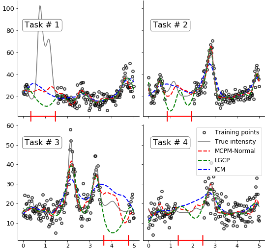
Figure 3: Four related tasks evaluated at 200 evenly spaced points in $[-1.5,1.5]$. |-| denote the 50 contiguous observations removed from the training set of each task.

Table 1: Performance on the missing intervals. mcpm-n and mcpm-gp denote independent and correlated prior respectively. Time in seconds per epoch.

	rmse				nlpl				cpu
	1	2	3	4	1	2	3	4	time
mcpm-n	38.61	7.86	5.71	4.68	20.99	3.75	3.31	3.02	0.18
mcpm-gp	38.58	7.69	5.70	4.71	20.95	3.70	3.31	3.03	0.25
lgcp	48.17	14.32	11.83	5.38	43.40	8.78	8.98	3.27	0.32
icm	39.07	7.96	7.88	6.03	21.81	3.76	3.77	3.38	0.52

Other GP-modulated Poisson processes: Rather than using a gp prior over the log intensity, different transformations of the latent gps have been considered as alternatives to model point data. For example, in the Permanental process, a gp prior is used over the squared root of the intensities (Walder and Bishop,, 2017; Lloyd et al.,, 2015; Lian et al.,, 2015; Lloyd et al.,, 2016; John and Hensman,, 2018). Similarly, a sigmoidal transformation of the latent gps was studied by Adams et al., (2009) and used in conjunction with convolution processes by Gunter et al., (2014). Permanental and Sigmoidal Cox processes are very different from lgcp/mcpm both in terms of statistical and computational properties. There is no conclusive evidence in the literature on which model provides a better characterisation of point processes and under what conditions. The mcpm likelihood introduces computational issues in terms of ell evaluation which in this work are solved by offering a closed form mgf function. On the contrary, permanental processes suffer from important identifiability issues such as reflection invariance and, together with sigmoidal processes, do not allow for a closed form prediction of the intensity function.

Among the inhomogeneous Cox process models, the only two multi-task frameworks are Gunter et al., (2014) and Lian et al., (mtpp, 2015). The former suffers from high computational cost due to the use of expensive mcmc schemes scaling with $\mathcal{O}(PN^{3})$. In addition, while the framework is develop for an arbitrary number of latent functions, a single latent function is used in all of the presented experiments. mtpp restricts the input space to be unidimensional and does not handle missing data. Furthermore, none of these two methods can handle spatial segregation (btb experiment) through a shared global mean function or a single latent function.

5 Experiments

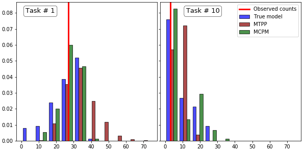
Figure 4: s2 dataset. Predicted empirical distribution of event counts for two tasks.

We first analyse mcpm on two synthetic datasets. In the first one, we illustrate the transfer capabilitites in a missing data setting comparing against lgcp and icm. In the second one, we assess the predictive performance against the mtpp model which cannot handle missing data. We then proceed to model two real world datasets that exhibit very different correlation structures. The first one includes spatially segregated tasks while the second one is characterized by strong positive correlation between tasks.

Baselines We offer results on both complete and incomplete data settings while comparing against mlgcp (Taylor et al.,, 2015), a variational lgcp model (Nguyen and Bonilla,, 2014) and a variational formulation of icm with Poisson likelihood implemented in GPflow (Matthews et al.,, 2017; Hensman et al.,, 2015).

Performance measures We compare the algorithms evaluating the root mean square error (rmse), the negative log predicted likelihood (nlpl) and the empirical coverage (ec) of the posterior predictive counts distribution. rmse and nlpl values for the $p$-th task are computed as $\textsc{rmse}_{p}=\sqrt{\frac{1}{N}\sum_{n=1}^{N}\left(y_{np}-\mathbb{E}(\lambda_{np})\right)^{2}}$ and $\textsc{nlpl}_{p}=-\frac{1}{S}\sum_{s=1}^{S}\frac{\sum_{n=1}^{N}\log p(y_{np}|\lambda_{np}^{s})}{n}$ where $\mathbb{E}(\lambda_{np})$ represents the posterior mean estimate for the $p$-th intensity at $\mathbf{x}_{n}$ and $S$ denotes the number of samples from the variational distributions $q(\mathbf{F})$ and $q(\mathbf{W})$. The ec is constructed by drawing random subregions from the training (in-sample) or the test set (out-of-sample) and evaluating the coverage of the 90% ci of the posterior ($p(N|\mathcal{D})$) and predictive ($p(N^{*}|\mathcal{D})$) counts distribution for each subregion $B$ (Leininger et al.,, 2017). These are in turn obtained by simulating from $N^{(l)}(B)\sim\text{Poisson}(\lambda^{(l)}(B))$ for $l=1,...,L$ with $\lambda^{(l)}(B)$ denoting the $l$-th sample from the intensity posterior and predictive distribution. The presented results consider $L=100$ and consistent results were found when changing this value. In terms of subregions selection, we fix their size, say $Z$, and randomly selected $L$ of them among all the possible areas of size $Z$ in the training or test set. $\textsc{ec}=1$ when all cis contain the ground truth. Finally, in order to assess transfer in the 2D experiments, we partition the spatial extent in $Z$ subregions and create missing data “folds” by combining non-overlapping regions, one for each task. We repeat the experiment $Z$ times until each task’s overall spatial extend is covered thus accounting for areas of both high and low intensity.

Table 2: s2 dataset. Performance on the test intervals. Time in seconds per epoch.

	nlpl										cpu
	1	2	3	4	5	6	7	8	9	10	time
mcpm-n	1.47	1.46	0.95	0.17	1.30	1.39	1.52	0.70	1.58	0.58	0.03
mcpm-gp	1.52	1.80	0.96	0.13	1.29	1.37	1.61	0.65	1.50	0.76	0.03
mtpp	1.60	3.05	1.13	0.15	1.24	1.44	1.49	1.13	1.70	0.52	5.97

Synthetic missing data experiment (s1) To illustrate the transfer capabilities of mcpm we construct four correlated tasks by sampling from a multivariate point process with final intensities obtained as the linear combination of two latent functions via task-specific mixing weights (Fig. 3). The final count observations are obtained by adding noise to the Poisson counts generated through the constructed intensities. When using a coupled prior over the weights, we consider covariates describing tasks (e.g. minimum and maximum values) as inputs. mcpm is able to reconstruct the task intensities in the missing data regions by learning the inter-task correlation and transferring information across tasks. Importantly, it significantly outperforms competing approaches for all tasks in terms of ec (see supplement) and nlpl. In addition, it has a lower rmse for $\nicefrac{{3}}{{4}}$ of the tasks (Tab. 1) while being $\approx$ 3 times faster than icm.

Synthetic comparison to mtpp (s2) To assess the predictive capabilities of mcpm against mtpp, which cannot handle missing data, we replicate the synthetic example proposed by Lian et al., (2015) (§6.1). We train the models with the observations in the interval $[0,80]$ and predict in the interval $[80,100]$. Fig. 4 shows how mcpm better recovers the true model event counts distribution with respect to mtpp. We found mcpm to outperform mtpp in terms of nlpl, ec and rmse for $\nicefrac{{7}}{{10}}$ tasks, see Tab 2 , Fig 4 and the supplementary material.

Table 3: Upper: crime dataset. Performance on the missing regions. Time in seconds per epoch. Lower values of nlpl are better. Lower: In-sample/Out-of-sample 90% ci coverage for the predicted event counts distributions. Higher values of ec are better.

	Standardized nlpl (per cell)							cpu
	1	2	3	4	5	6	7	time
mcpm-n	0.56	0.91	0.66	1.09	0.85	10.29	0.42	2.85
	(0.10)	(0.27)	(0.30)	(0.27)	(0.52)	(2.51)	(0.05)
mcpm-gp	0.72	0.75	0.94	1.53	0.57	18.76	0.58	3.11
	(0.18)	(0.18)	(0.55)	(0.52)	(0.19)	(8.25)	(0.12)
lgcp	9.90	9.32	19.34	5.30	18.18	36.73	9.68	2.87
	(3.66)	(2.41)	(11.45)	(1.02)	(8.65)	(4.02)	(2.67)
icm	0.87	1.36	0.91	1.19	0.69	12.30	0.93	44.13
	(0.27)	(0.35)	(0.45)	(0.40)	(0.11)	(3.02)	(0.17)

	Empirical Coverage (ec)
	1	2	3	4	5	6	7
mcpm-n	0.99/0.80	1.00/0.73	0.97/0.71	1.00/0.73	0.98/0.61	1.00/1.00	0.99/0.87
mcpm-gp	1.00/0.87	1.00/0.74	1.00/0.71	1.00/0.95	1.00/0.88	0.80/1.00	1.00/0.85
lgcp	0.86/0.29	0.76/0.20	0.86/0.29	0.82/0.37	0.68/0.25	0.94/0.00	0.83/0.21
icm	0.68/0.73	0.75/0.50	0.64/0.52	0.79/0.65	0.59/0.78	0.93/0.86	0.841/0.64

5.1 Crime events in NYC

In this section we demonstrate the performance, transfer capabilities and scalability of mcpm on a real-world dataset recording different crimes in nyc (crime). The dataset includes latitude and longitude locations of burglaries (1), felony assaults (2), grand larcenies (3), grand larcenies of motor vehicle (mv, 4), petit larcenies (5), petit larcenies of mv (6) and robberies (7) reported in 2016. The data are discretized into a 32$\times$32 regular grid (Fig.5). Lack of ground truth intensities typically restricts quantitative measures of generalization and hence we focus on validating and comparing mcpm from two different perspectives: i) using complete data so as to assess the quality of the recovered intensities as well as the computational complexity and scalability gains over mlgcp; and ii) using missing data so as to validate the transfer capabilities of mcpm when compared with lgcp and icm.

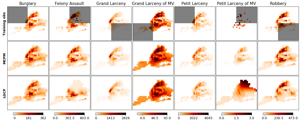
Figure 5: crime dataset. Estimated surface when introducing missing data in the shaded regions. Row 1: Counts of crime events on a regular grid. Row 2: mcpm Row 3: lgcp.

Complete/Missing Data Experiments We first consider a full-data experiment and we spatially interpolate the crime surfaces running mcpm with four latent functions characterized by Matérn 3/2 kernels. We repeat the experiment with mlgcp setting the algorithm parameters as suggested by Taylor et al., (2015). Similar results are obtained with the two methods (see Fig. (8) in the supplement for a visualisation of the estimated intensity surfaces). However, in terms of computational gains, an mlgcp run takes $\approx$ 14 hrs while mcpm requires $\approx$ 2 hrs.

To assess transfer, we keep the same experimental settings and introduce missing data regions by partitioning the spatial extent in 4 subregions as explained above. The shaded regions in Fig. 5 represent one possible configuration of the missing data across tasks. mcpm successfully transfers information across tasks (Fig. 5) thereby recovering, for all crime types, the signal in the missing data regions. By exploiting task similarities, the algorithm outperforms competing approaches in all of the tasks, in terms of ec, nlpl (Tab. 3) and rmse (see the supplementary material.) Finally, mcpm significantly outruns icm in terms of algorithm efficiency. mcpm-n converges in 1.19 hrs (1500 epochs) on a Intel Core i7-6t00u cpu (3.40GHz, 8gb of ram) while icm needs 12.26 hrs (1000 epochs).

Table 4: Upper: rmse and nlpl on btb with missing data. Time in seconds per epoch. Lower values of nlpl are better. Lower: In-sample/Out-of-sample 90% ci coverage for the predicted event counts distributions. Higher values of ec are better.

	rmse				nlpl (per cell)				cpu
	gt 9	gt 12	gt 15	gt 20	gt 9	gt 12	gt 15	gt 20	time
mcpm-n	0.83	0.24	0.28	0.29	1.23	0.20	0.33	0.35	7.73
	(0.15)	(0.07)	(0.07)	(0.10)	(0.40)	(0.07)	(0.11)	(0.16)
mcpm-gp	0.81	0.22	0.27	0.27	1.42	0.27	0.41	0.58	7.63
	(0.14)	(0.08)	(0.07)	(0.09)	(0.42)	(0.09)	(0.14)	(0.24)
lgcp	1.37	0.61	0.63	1.24	1.70	0.48	0.72	0.86	8.76
	(0.33)	(0.13)	(0.12)	(0.56)	(0.39)	(0.11)	(0.17)	(0.36)
icm	0.91	0.21	0.32	7.24	1.44	0.18	0.34	0.37	67.06
	(0.15)	(0.07)	(0.08)	(5.48)	(0.40)	(0.06)	(0.10)	(0.14)

	Empirical Coverage (ec)
	gt 9	gt 12	gt 15	gt 20
mcpm-n	0.87/0.92	0.97/0.99	0.93/0.96	0.95/1.00
mcpm-gp	0.93/0.91	0.98/0.98	0.97/0.98	0.97/0.99
lgcp	0.91/0.79	0.97/0.98	0.97/0.97	0.96/0.98
icm	0.90/0.84	0.96/0.98	0.95/0.96	0.96/0.96

5.2 Bovine Tuberculosis (btb) in Cornwall

We showcase the performance of mcpm on the btb dataset (Diggle et al.,, 2013; Taylor et al.,, 2015) consisting of locations of btb incidents in Cornwall, uk (period 1989–2002) and covariates measuring cattle density, see first row in Fig. 6. We follow Diggle et al., (2013) and only consider the four most common btb genotypes (gt: 9, 12, 15 and 20).

Complete Data Experiments: We estimate the four btb intensities by fitting an mcpm with four latent functions and Matérn 3/2 kernels. We initialise the kernel lenghtscales and variances to 1. For direct comparison, we train the mlgcp model following the grid size, prior, covariance and mcmc settings by Taylor et al., (2015). We run the mcmc chain for 1M iterations with a burn in of 100K and keep 1K thinned steps. Following Diggle et al., (2013), in Fig. 6 we report the probability surfaces computed as $\pi_{p}(x)=\lambda_{p}(x)/\sum_{p=1}^{P}\lambda_{p}(x)$ where $\lambda_{p}(x)$ is the posterior mean of the intensity for task $p$ at location $x$. Estimated intensities surfaces can be found in the supplementary material.

The probability surfaces are comparable with both approaches characterizing well the high and low intensities albeit varying at the level of smoothness. In terms of computational gains we note that mlgcp takes $\approx$ 30 hrs for an interpolation run on the four btb tasks while mcpm only requires $\approx$ 8 hrs. The previously reported (Diggle et al.,, 2013) slow mixing and convergence problems of the chain, even after millions of mcmc iterations, renders mlgcp problematic for application to large-scale multivariate point processes. Finally, the built-in assumption of a single common gp latent process across tasks limits the number and the type of inter-task correlations that we can identify and model efficiently.

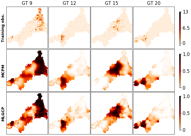
Figure 6: Estimated conditional probabilities on btb (Second row: mcpm, Third row:mlgcp) in the complete data setting. Estimated intensity surfaces are available in the supplementary material.

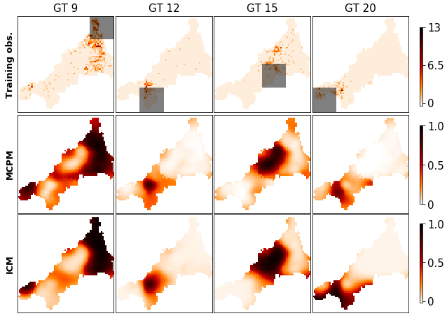
Figure 7: First row: Counts of the btb incidents on a 64$\times$64 grid. Shaded areas represent missing data regions. Estimated conditional probabilities by mcpm (second row) and by icm (third row).

Missing Data Experiments:Transfer is evaluated by partitioning the space into 16 suregions and constructing missing data regions as explained above. The shaded regions in the first row of Fig. 7 represent one such fold of the missing areas across tasks. We provide average quantitative metrics across folds for an mcpm with four latent functions, Matérn 3/2 kernels and $30\%$ of the training inputs as inducing inputs. As in the complete data setting, we report estimated conditional probabilities in Fig. 7. mcpm manages to recover the overall behaviour of the process in the missing regions showing significant transfer of information across spatially segregated tasks while avoiding negative transfer in the case of negative spatial correlation. mcpm outperforms lgcp across all tasks and icm on $\nicefrac{{3}}{{4}}$ of the tasks (Tab. 4) while achieving the highest ec both in-sample and out-of-sample. In addition, mcpm has a significant computational advantage: it converges in 3.18 hrs (1500 epochs) while icm converges in 18.63 hrs (1000 epochs).

6 Conclusions and Discussion

We proposed a new multi-task learning framework for modeling correlated count data based on lgcp models. We consider observations on different tasks as being drawn from distinct lgcps with correlated intensities determined by linearly combined gps through task-specific random weights. By considering stochastic weights, we allow for the incorporation of additional dependencies across tasks while providing better uncertainty quantification. We derive closed-form expressions for the moments of the intensity functions and use them to develop an efficient variational algorithm that is order of magnitude faster than the current state of the art. We show how mcpm achieves the state of the art performance on both synthetic and real datasets providing a more flexible and up to 15 times faster methodology compared to the available lgcp multivariate methods. Future work will focus on increasing the interpretability of the mixing weights. For instance, placing an alternative sparse prior distribution (Titsias and Lázaro-Gredilla,, 2011) on $\mathbf{W}$ would induce sparsity and thus act as a model selection mechanism for $Q$. However, introducing a more complex prior on $\mathbf{W}$ would also break the tractability of the variational objective and would require further approximations.

Acknowledgments

This work was supported by the EPSRC grant EP/L016710/1, The Alan Turing Institute under EPSRC grant EP/N510129/1 and the Lloyds Register Foundation programme on Data Centric Engineering.

References

- Abadi et al., (2016) Abadi, M., Agarwal, A., Barham, P., Brevdo, E., Chen, Z., Citro, C., Corrado, G. S., Davis, A., Dean, J., Devin, M., et al. (2016). Tensorflow: Large-scale machine learning on heterogeneous distributed systems. arXiv preprint arXiv:1603.04467.
- Adams et al., (2009) Adams, R. P., Murray, I., and MacKay, D. J. (2009). Tractable nonparametric bayesian inference in poisson processes with gaussian process intensities. Proceedings of the 26th Annual International Conference on Machine Learning, pages 9–16.
- Álvarez and Lawrence, (2011) Álvarez, M. A. and Lawrence, N. D. (2011). Computationally efficient convolved multiple output gaussian processes. Journal of Machine Learning Research, 12(May):1459–1500.
- Alvarez et al., (2010) Alvarez, M. A., Luengo, D., Titsias, M. K., and Lawrence, N. D. (2010). Efficient multioutput gaussian processes through variational inducing kernels. Artificial Intelligence and Statistics, 9:25–32.
- Alvarez et al., (2012) Alvarez, M. A., Rosasco, L., Lawrence, N. D., et al. (2012). Kernels for vector-valued functions: A review. Foundations and Trends® in Machine Learning, 4(3):195–266.
- Bonilla et al., (2008) Bonilla, E. V., Chai, K. M., and Williams, C. (2008). Multi-task gaussian process prediction. Advances in neural information processing systems, pages 153–160.
- Bonilla et al., (2016) Bonilla, E. V., Krauth, K., and Dezfouli, A. (2016). Generic inference in latent Gaussian process models. arXiv preprint arXiv:1609.00577.
- Caruana, (1998) Caruana, R. (1998). Multitask learning. In Learning to learn, pages 95–133. Springer.
- Cox, (1955) Cox, D. R. (1955). Some statistical methods connected with series of events. Journal of the Royal Statistical Society. Series B (Methodological), pages 129–164.
- Craig, (1936) Craig, C. C. (1936). On the frequency function of xy. The Annals of Mathematical Statistics, 7(1):1–15.
- Dezfouli and Bonilla, (2015) Dezfouli, A. and Bonilla, E. V. (2015). Scalable inference for gaussian process models with black-box likelihoods. Advances in Neural Information Processing Systems, pages 1414–1422.
- Diggle et al., (2013) Diggle, P. J., Moraga, P., Rowlingson, B., and Taylor, B. M. (2013). Spatial and spatio-temporal log-gaussian cox processes: Extending the geostatistical paradigm. Statistical Science, pages 542–563.
- Flaxman et al., (2015) Flaxman, S., Wilson, A., Neill, D., Nickisch, H., and Smola, A. (2015). Fast kronecker inference in gaussian processes with non-gaussian likelihoods. International Conference on Machine Learning, pages 607–616.
- Gal et al., (2014) Gal, Y., van der Wilk, M., and Rasmussen, C. (2014). Distributed variational inference in sparse Gaussian process regression and latent variable models. Neural Information Processing Systems.
- Gunter et al., (2014) Gunter, T., Lloyd, C., Osborne, M. A., and Roberts, S. J. (2014). Efficient bayesian nonparametric modelling of structured point processes. Proceedings of the Thirtieth Conference on Uncertainty in Artificial Intelligence, pages 310–319.
- Hensman et al., (2015) Hensman, J., Matthews, A., and Ghahramani, Z. (2015). Scalable variational Gaussian process classification. Artificial Intelligence and Statistics.
- John and Hensman, (2018) John, S. and Hensman, J. (2018). Large-scale cox process inference using variational fourier features. arXiv preprint arXiv:1804.01016.
- Jordan et al., (1999) Jordan, M. I., Ghahramani, Z., Jaakkola, T. S., and Saul, L. K. (1999). An introduction to variational methods for graphical models. Machine learning, 37(2):183–233.
- Leininger et al., (2017) Leininger, T. J., Gelfand, A. E., et al. (2017). Bayesian inference and model assessment for spatial point patterns using posterior predictive samples. Bayesian Analysis, 12(1):1–30.
- Lian et al., (2015) Lian, W., Henao, R., Rao, V., Lucas, J., and Carin, L. (2015). A multitask point process predictive model. International Conference on Machine Learning, pages 2030–2038.
- Lloyd et al., (2016) Lloyd, C., Gunter, T., Nickson, T., Osborne, M., and Roberts, S. J. (2016). Latent point process allocation. Journal of Machine Learning Research.
- Lloyd et al., (2015) Lloyd, C., Gunter, T., Osborne, M. A., and Roberts, S. J. (2015). Variational Inference for Gaussian Process Modulated Poisson Processes. International Conference on Machine Learning.
- Matthews et al., (2017) Matthews, A. G. d. G., van der Wilk, M., Nickson, T., Fujii, K., Boukouvalas, A., León-Villagrá, P., Ghahramani, Z., and Hensman, J. (2017). GPflow: A Gaussian process library using TensorFlow. Journal of Machine Learning Research, 18(40):1–6.
- Møller et al., (1998) Møller, J., Syversveen, A. R., and Waagepetersen, R. P. (1998). Log gaussian cox processes. Scandinavian journal of statistics, 25(3):451–482.
- Nguyen and Bonilla, (2014) Nguyen, T. V. and Bonilla, E. V. (2014). Automated variational inference for Gaussian process models. Advances in Neural Information Processing Systems, pages 1404–1412.
- Schmidt and Gelfand, (2003) Schmidt, A. M. and Gelfand, A. E. (2003). A bayesian coregionalization approach for multivariate pollutant data. Journal of Geophysical Research: Atmospheres, 108(D24).
- Shirota and Gelfand, (2016) Shirota, S. and Gelfand, A. E. (2016). Inference for log Gaussian Cox processes using an approximate marginal posterior. arXiv preprint arXiv:1611.10359.
- Taylor et al., (2015) Taylor, B., Davies, T., Rowlingson, B., and Diggle, P. (2015). Bayesian inference and data augmentation schemes for spatial, spatiotemporal and multivariate log-Gaussian Cox processes in r. Journal of Statistical Software, 63:1–48.
- Teh et al., (2005) Teh, Y. W., Seeger, M., and Jordan, M. I. (2005). Semiparametric latent factor models. Artificial Intelligence and Statistics.
- Titsias, (2009) Titsias, M. K. (2009). Variational learning of inducing variables in sparse gaussian processes. Artificial Intelligence and Statistics, 5:567–574.
- Titsias and Lázaro-Gredilla, (2011) Titsias, M. K. and Lázaro-Gredilla, M. (2011). Spike and slab variational inference for multi-task and multiple kernel learning. Advances in neural information processing systems, pages 2339–2347.
- Walder and Bishop, (2017) Walder, C. J. and Bishop, A. N. (2017). Fast Bayesian intensity estimation for the permanental process. International Conference on Machine Learning.
- Williams and Rasmussen, (2006) Williams, C. K. and Rasmussen, C. E. (2006). Gaussian processes for machine learning. the MIT Press, 2(3):4.
- Wilson et al., (2011) Wilson, A. G., Knowles, D. A., and Ghahramani, Z. (2011). Gaussian process regression networks. International Conference on Machine Learning.