Static Casimir Condensate of Conformal Scalar Field in Friedmann Universe

Abstract

The quantum Casimir condensate of a conformal massive scalar field in a compact Friedmann universe is considered in the static approximation. The Abel–Plana formula is used for renormalization of divergent series in the condensate calculation. A differential relation between the static Casimir energy density and static Casimir condensate is derived.

PACS Nos.: 11.25.Hf, 11.30.Qc

1 Introduction

Quantum field condensates are known to appear in systems with spontaneous symmetry breaking such as the Standard Model and QCD. In particular, the Coleman–Weinberg mechanism [1] allows emergence of a finite field condensate starting from a conformal-invariant semi-classical Lagrangian. The quantum condensate mechanism of the origin of Higgs boson mass without explicit conformal symmetry breaking was proposed in Ref. [2]. But to define of the conformal field condensate value, an additional physical condition is required. One of the possibilities is to relate the emergent finite value of the condensate to certain boundary conditions of the system like in the Casimir effect. In the present paper we will consider the case of a scalar field in a closed manifold. The topological Casimir effect will be treated. A non-trivial topology of the space provides the rule how to fix the renormalization condition in the calculations. Contrary to the case of the standard Casimir effect, no border or boundary condition is imposed.

The Casimir effect plays an essential role in cosmological models and in particle physics [3]. Besides of the Casimir energy, the Casimir condensates of quantum fields deserve a study, especially in the early stage of the Universe. The Casimir condensate can be defined as vacuum mean value of two field operators in one point of the manifold. It corresponds to a tadpole (vacuum bubble) Feynman diagram without external legs. This object contributes to the universe vacuum energy and its treatment is crucial for cosmological applications [4].

In the conformally static universe the calculation of the energy density, pressure, and the density number of the boson pairs created during the evolution of the universe from the singular initial state was performed in Ref. [5]. However, the Casimir energy-momentum tensor of a boson field has singularity at the zero scale factor value, $a=0$, which corresponds to the initial moment of the universe evolution. To avoid the initial cosmological singularity, one can exploit conformal transformations to the static universe that is a sphere of the present day radius $a_{0}$. The conformal transformation should be applied also to quantum fields simultaneously. The calculation of the Casimir condensate should be considered in conformal variables also.

From the conformal cosmological conception, the universe is not expanded but the elementary particles masses turn out to be depend on time, see e.g. Ref. [6]. The redshift of galactic spectrum and the modern Hubble diagram can be interpreted [7, 8, 9] within the General Relativity in conformal variables without introducing Dark Energy. The transition to the conformal variables has a considerable advantage since the initial cosmological singularity doesn’t appear there. The procedures of Hamiltonian reduction and deparametrization in Geometrodynamics by passing to the conformal spatial metric, were recently analyzed in Ref. [10].

There are various effective methods of regularization and renormalization of ultraviolet divergences. In particular, several such methods were developed to treat the Casimir effect in different cases, see e.g. book [3]. In particular for the case of the topological Casimir effect, extraction of the finite value of a boson condensate can be achieved by subtraction from a divergent sum defined in the Friedmann space the corresponding divergent integral defined in the Minkowskian tangent space. The Abel–Plana formula from the theory of analytical functions can be applied for this purpose, see Ref. [5].

2 Conformal massive scalar field

The conformal spacetime metric of a Friedmann universe ${\cal M}=\mathbb{R}^{1}\times S^{3}$ reads

$$ds^{2}=a^{2}(\eta)\left(-d\eta^{2}+d\chi^{2}+\sin^{2}\chi(d\theta^{2}+\sin^{2}\theta d\phi^{2})\right),$$ (1)

where $\eta$ is the conformal time; $a(\eta)$ is the conformal scale factor having the sense of the $S^{3}$-sphere radius; $\chi$, $\theta$, and $\phi$ are dimensionless angular coordinates on the sphere. The Lagrangian density of a massive scalar field $\varphi(x)$ with a conformal coupling has the form [11, 12]

$${\cal L}=-\frac{1}{2}\sqrt{-g}(x)\left(g^{\mu\nu}(x)\nabla_{\mu}\varphi(x)\nabla_{\nu}\varphi(x)+m^{2}\varphi^{2}(x)+\frac{1}{6}R(x)\varphi^{2}(x)\right).$$ (2)

Here, $g$ is the determinant of the spacetime metric; $g^{\mu\nu}$ are components of the inverse metric tensor; $\nabla_{\mu}$ is the covariant derivative; $m$ is the bare mass of the field. The scalar curvature of the spacetime (1) is

$$R(\eta)=\frac{6}{a^{3}}(a^{\prime\prime}+a),$$ (3)

where the prime denotes differentiation with respect to $\eta$. The Klein–Fock–Gordon equation

$$\left(-g^{\mu\nu}\nabla_{\mu}\nabla_{\nu}+m^{2}+\frac{1}{6}R\right)\varphi(x)=0$$ (4)

takes the form

$$\varphi^{\prime\prime}+2\frac{a^{\prime}}{a}\varphi^{\prime}-\triangle\varphi+\left(m^{2}a^{2}+\frac{a^{\prime\prime}}{a}+1\right)\varphi=0,$$ (5)

where $\triangle$ is the angular part of the Laplace operator on a 3-sphere with the unit radius.

Let us perform the transformation to the conformal metric $\tilde{g}_{\mu\nu}(x)$ and the conformal field $\tilde{\varphi}(x)$ according to their conformal weights:

$$g_{\mu\nu}(x)=\left(\frac{a(\eta)}{a_{0}}\right)^{2}\tilde{g}_{\mu\nu}(x),\qquad\varphi(x)=\left(\frac{a_{0}}{a(\eta)}\right)\tilde{\varphi}(x).$$ (6)

The static spacetime interval corresponds to the present day radius $a_{0}$ of the universe

$$d\tilde{s}^{2}=a_{0}^{2}(-d\eta^{2}+d\chi^{2}+\sin^{2}\chi(d\theta^{2}+\sin^{2}\theta d\phi^{2}))$$ (7)

with the curvature $\tilde{R}=6/a_{0}^{2}$. Transformation (6) leads to the Klein–Fock–Gordon equation for the conformal scalar field $\tilde{\varphi}(x)$ with a variable mass $m(\eta)=m\cdot a(\eta)$

$$\tilde{\varphi}^{\prime\prime}-\triangle\tilde{\varphi}+(m^{2}a^{2}+1)\tilde{\varphi}=0.$$ (8)

The transition to the conformal variables leads to observable quantities with regular behavior at $a=0$. In the corresponding quantum theory it yields finite physical results [5]. The eigenfunctions of (8) can be presented in the factorized form

$$\tilde{\varphi}_{J}(x)=g_{\lambda}(\eta)Y_{J}({\bf x}).$$ (9)

Here, the eigenfunctions $Y_{J}(\chi,\theta,\phi)$ of the Laplace–Beltrami operator [3] are spherical functions

$$(\triangle+k^{2}_{J})Y_{J}=0,$$ (10)

forming the orthonormal basis of unitary representations of the isometry group of the $S^{3}$-sphere

$$Y_{J}(\chi,\theta,\phi)=\frac{1}{\sqrt{\sin\chi}}\sqrt{\frac{\lambda(\lambda+l)!}{(\lambda-l+1)!}}P^{-l-1/2}_{\lambda-1/2}(\cos\chi)Y_{lM}(\theta,\phi),$$ (11)

the combined index $J\equiv\{\lambda,l,M\}$ runs over values

$$\lambda=1,2,3,\ldots;\qquad l=0,1,2,\ldots,\lambda-1;\qquad-l\leq M\leq l.$$ (12)

The eigenvalues of Eq. (10) are $k_{J}^{2}=\lambda^{2}-1$. The equation of the oscillator type for $g_{\lambda}(\eta)$ is obtained after substitution of (9) into the Klein–Fock–Gordon equation (8)

$$\frac{d^{2}}{d\eta^{2}}g_{\lambda}(\eta)+\omega^{2}(\eta)g_{\lambda}(\eta)=0,\qquad\omega^{2}(\eta)\equiv\lambda^{2}+m^{2}a^{2}(\eta).$$ (13)

To find solutions of the above equation, it is necessary to choose a definite evolution law for the scale factor $a(\eta)$ [5].

The functions

$$\tilde{\varphi}_{J}^{(+)}(x)=\frac{1}{\sqrt{2}}g_{\lambda}(\eta)Y_{J}^{*}({\bf x}),\qquad\tilde{\varphi}_{J}^{(-)}(x)=\frac{1}{\sqrt{2}}g_{\lambda}^{*}(\eta)Y_{J}({\bf x})$$ (14)

compose the complete set of classical solutions of the Klein–Fock–Gordon equation (8) if the Wronskian is equal to

$$g_{\lambda}{g_{\lambda}^{*}}^{\prime}-{g_{\lambda}}^{\prime}g_{\lambda}^{*}=-2\imath.$$ (15)

3 Casimir condensate of a massive scalar field

The vacuum state is defined by the condition $a_{J}^{(-)}|0>=0$. The operator commutation relations are

$$[a_{J}^{(-)},a_{J^{\prime}}^{(+)}]=\delta_{JJ^{\prime}},\qquad[a_{J}^{(+)},a_{J^{\prime}}^{(+)}]=[a_{J}^{(-)},a_{J^{\prime}}^{(-)}]=0.$$ (16)

The quantum field operator is then combined as the sum

$$\tilde{\varphi}(x)=\sum\limits_{J}\left(\tilde{\varphi}_{J}^{(-)}(x)a_{J}^{(-)}+\tilde{\varphi}_{J}^{(+)}(x)a_{J}^{(+)}\right).$$ (17)

The conditions of orthonormality for the functions read

$$(\tilde{\varphi}_{J}^{(\pm)},\tilde{\varphi}_{J^{\prime}}^{(\pm)})=\mp\delta_{JJ^{\prime}},\qquad(\tilde{\varphi}_{J}^{(\pm)},\tilde{\varphi}_{J^{\prime}}^{(\mp)})=0,$$ (18)

where the scalar product of functions is defined over a finite volume $V$ as

$$(f,g)\equiv\int_{V}\,d^{3}x\sqrt{\gamma}\left(f^{*}\frac{\partial}{\partial t}g-g^{*}\frac{\partial}{\partial t}f\right).$$ (19)

We define the quantum Casimir condensate as the vacuum mean value of two operators in one point:

$$<0|\tilde{\varphi}(x)\tilde{\varphi}(x)|0>=\sum\limits_{J,J^{\prime}}\tilde{\varphi}_{J}^{(-)}(x)\tilde{\varphi}_{J^{\prime}}^{(+)}(x)<0|a_{J}^{(-)}a_{J^{\prime}}^{(+)}|0>=\frac{1}{2}\sum\limits_{J}|g_{\lambda}(\eta)|^{2}|Y_{J}({\bf x})|^{2}.$$ (20)

By applying the formula for summation over quantum numbers $(l,M)$

$$\sum\limits_{l,M}|Y_{J}({\bf x})|^{2}=\frac{\lambda^{2}}{2\pi^{2}},$$

we get

$$<0|\tilde{\varphi}(x)\tilde{\varphi}(x)|0>=\frac{1}{4\pi^{2}}\sum_{\lambda=1}^{\infty}\lambda^{2}|g_{\lambda}(\eta)|^{2}.$$ (21)

In this paper the effects of vacuum polarization and particle creation are not considered. Restricting our attention to the pure static Casimir contribution into the quantum condensate in the case of the quasi-static condition $(a^{\prime}=0)$ [3], the solution to the oscillator equation (13) can be given as

$$g_{\lambda}(\eta)=\frac{e^{\imath\omega_{\lambda}\eta}}{\sqrt{\omega_{\lambda}}}.$$ (22)

Thus one gets the divergent series

$$<0|\tilde{\varphi}(x)\tilde{\varphi}(x)|0>=\frac{1}{4\pi^{2}}\sum_{\lambda=1}^{\infty}\frac{\lambda^{2}}{\sqrt{\lambda^{2}+m^{2}a^{2}}}.$$ (23)

Now the problem is formulated for a scalar field with mass $(ma)$ in a static Einstein universe $\mathbb{R}^{1}\times S^{3}$, where $S^{3}$ is a sphere of radius $a_{0}$. For renormalization of the series the Abel–Plana formula can be applied [3]

$${\rm ren}\left\{\sum_{\lambda=0}^{\infty}F(\lambda)\right\}\equiv\sum\limits_{\lambda=0}^{\infty}F(\lambda)-\int\limits_{0}^{\infty}dt\,F(t)=\frac{F(0)}{2}+\imath\int\limits_{0}^{\infty}dt\,\frac{F(\imath t)-F(-\imath t)}{\exp(2\pi t)-1},$$ (24)

where $F(\lambda)$ is an analytic function. From the physical point of view, we have a finite difference between the divergent sum of $F(\lambda)$ defined in the Friedmann spacetime and the corresponding divergent integral of this function $F(t)$ defined in the tangent Minkowskian one. Subtraction of the contribution of the quantum condensate in the 3-dimensional Minkowskian space tangent to the $S^{3}$, leads to the renormalized result in the form of the following convergent integral:

$$\tilde{c}:=<0|\tilde{\varphi}(x)\tilde{\varphi}(x)|0>^{\rm ren}=-\frac{1}{2\pi^{2}}\int\limits_{ma}^{\infty}\frac{\lambda^{2}d\lambda}{\sqrt{\lambda^{2}-m^{2}a^{2}}(\exp(2\pi\lambda)-1)}.$$ (25)

In derivation of this formula, we kept in mind that the integrand function $F(\lambda)=\lambda^{2}/\sqrt{\lambda^{2}+m^{2}a^{2}}$ has branch points for $\lambda=\pm\imath ma$, so

$$F(\imath\lambda) = F(-\imath\lambda)=-\frac{\lambda^{2}}{\sqrt{m^{2}a^{2}-\lambda^{2}}},\qquad\lambda<ma,$$

$$F(\imath\lambda) = -F(-\imath\lambda)=\imath\frac{\lambda^{2}}{\sqrt{\lambda^{2}-m^{2}a^{2}}},\qquad\lambda>ma.$$

Integral (25) is limited from the bottom by the variable bare mass of the elementary particle. For the case of massless virtual particles, the regularized function in (25) coincides with distribution function for bosons with the effective temperature $T_{\rm eff}=\hbar c/(2\pi k_{B})$, where $k_{B}$ is the Boltzmann constant. For the massless case $(m=0)$, integration of (25) gives

$$\tilde{c}_{0}=-\frac{1}{2\pi^{2}}\int\limits_{0}^{\infty}\frac{\lambda d\lambda}{\exp(2\pi\lambda)-1}=\frac{1}{4\pi^{2}}{\rm ren}\sum\limits_{\lambda=1}^{\infty}\lambda=-\frac{1}{48\pi^{2}}.$$ (26)

For elementary particles with $ma\gtrsim 0.5$, the dominant energy condition $\epsilon\geq|p|$ is violated as discussed in Ref. [13]. This can lead to particle creation by gravitational field. The dependence of the dimensionless ratio of the conformal condensates (25) and (26) on the dimensionless variable mass ${\tilde{c}}/{\tilde{c}_{0}}={\tilde{c}}/{\tilde{c}_{0}}(ma)$ is regular, it is shown in Fig. 1.

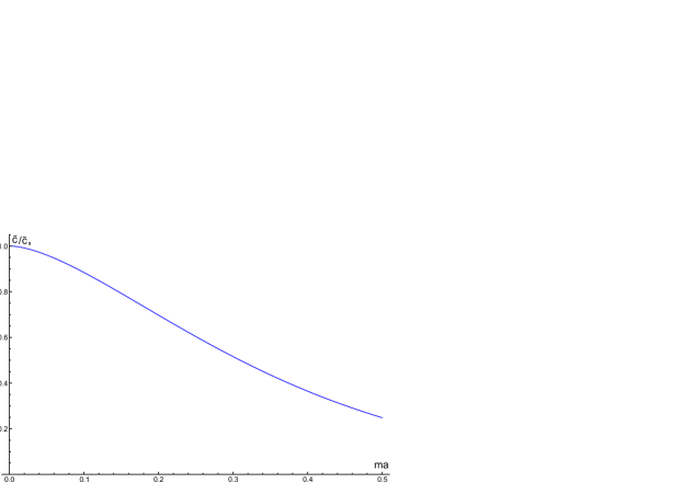
Figure 1: Casimir condensate of a conformal massive scalar field as a function of $ma$.

The renormalized value of the static Casimir energy density of the conformal scalar field [3] as the renormalized mean value of the corresponding component of the conformal energy-momentum tensor reads

$$\tilde{\epsilon}:=-\tilde{g}^{00}<0|\tilde{T}_{00}|0>^{\rm ren}=\frac{\hbar c}{2\pi^{2}a_{0}^{2}}\int\limits_{ma}^{\infty}d\lambda\,\frac{\lambda^{2}\sqrt{\lambda^{2}-m^{2}a^{2}}}{\exp(2\pi\lambda)-1}.$$ (27)

The condensate $\tilde{c}$ (25) and the corresponding energy density $\tilde{\epsilon}$ (27) of the massive conformal scalar field are related to each other. If one differentiates (27) with respect to the variable mass as a parameter, the relation is revealed

$$\frac{\partial\tilde{\epsilon}}{\partial(ma)}=-(ma)\frac{1}{2\pi^{2}a_{0}^{2}}\int\limits_{ma}^{\infty}\frac{\lambda^{2}d\lambda}{\sqrt{\lambda^{2}-m^{2}a^{2}}(\exp(2\pi\lambda)-1)}=\hbar c\left(\frac{ma}{a_{0}^{2}}\right)\tilde{c}.$$ (28)

Formula (28) can be rewritten also as

$$\frac{\partial\tilde{\epsilon}}{\partial(m^{2}a^{2})}=\frac{\hbar c}{2a_{0}^{2}}\tilde{c}.$$ (29)

4 Conclusions

In this way, we calculated the static Casimir condensate of a conformal massive scalar in a compact Friedmann universe. The differential relation between the energy density and the condensate is obtained. The Abel–Plana formula, used to renormalize the results, has a clear physical meaning. It is much more simple than the regularization procedure with a wavelength cutoff applied in Ref. [13]. The applied procedure can be extended for the case of spinor and vector fields. It would be also interesting to go beyond the conformally static approximation and consider the dynamics of the Casimir condensate depending on the universe scale factor $a(\eta)$ evolution.

References

- [1] S.R. Coleman and E.J. Weinberg, Phys. Rev. D 7, 1888 (1973).
- [2] A.B. Arbuzov, R.G. Nazmitdinov, A.E. Pavlov, V.N. Pervushin, A.F. Zakharov, Europhys. Lett. 113, 31001 (2016).
- [3] V.M. Mostepanenko and N.N. Trunov, The Casimir Effect and its Applications (Oxford University Press, 1997).
- [4] J. Martin, Comptes Rendus Physique 13, 566 (2012).
- [5] S.G. Mamaev, V.M. Mostepanenko, A.A. Starobinsky, Sov. Phys. JETP 43, 823 (1976).
- [6] J. Narlikar, Violent Phenomena in the Universe. (Oxford University Press, 1984).
- [7] A.F. Zakharov and V.N. Pervushin, Int. J. Mod. Phys. D 19, 1875 (2010).
- [8] A.E. Pavlov, RUDN J. Math. Inform. Sc. Phys. 25, 390 (2017).
- [9] V.N. Pervushin, A.B. Arbuzov, A.F. Zakharov, Phys. Part. Nucl. Lett. 14, 368 (2017).
- [10] A.B. Arbuzov, A.E. Pavlov, arXiv:1710.01528.
- [11] N.A. Chernikov, E.A. Tagirov, Ann. Inst. H. Poincar 9A, 109 (1968).
- [12] R. Penrose, Conformal treatment of infinity, in: Relativity, Groups and Topology, eds. C. DeWitt, B. DeWitt, (Gordon and Breach, 1964), p. 565.
- [13] L.H. Ford, Phys. Rev. D 14, 3304 (1976).