Stable Super-Resolution of Images: A Theoretical Study

Abstract

We study the ubiquitous super-resolution problem, in which one aims at localizing positive point sources in an image, blurred by the point spread function of the imaging device. To recover the point sources, we propose to solve a convex feasibility program, which simply finds a nonnegative Borel measure that agrees with the observations collected by the imaging device.

In the absence of imaging noise, we show that solving this convex program uniquely retrieves the point sources, provided that the imaging device collects enough observations. This result holds true if the point spread function of the imaging device can be decomposed into horizontal and vertical components, and if the translations of these components form a Chebyshev system, i.e., a system of continuous functions that loosely behave like algebraic polynomials.

Building upon recent results for one-dimensional signals [1], we prove that this super-resolution algorithm is stable , in the generalized Wasserstein metric, to model mismatch (i.e., when the image is not sparse) and to additive imaging noise. In particular, the recovery error depends on the noise level and how well the image can be approximated with well-separated point sources. As an example, we verify these claims for the important case of a Gaussian point spread function. The proofs rely on the construction of novel interpolating polynomials —which are the main technical contribution of this paper— and partially resolve the question raised in [2] about the extension of the standard machinery to higher dimensions.

1 Introduction

Consider an unknown number of point sources with unknown locations and amplitudes. An imaging mechanism provides us with a few noisy measurements from which we wish to estimate the locations and amplitudes of these sources. Because of the finite resolution of any imaging device, poorly separated sources are indistinguishable without using an appropriate localization technique that would take into account the sparse structure within the image.

This super-resolution problem of localizing point sources finds various applications in, for instance, astronomy [3], geophysics [4], chemistry, medicine, microscopy and neuroscience [5, 6, 7, 8, 9, 10, 11]. In this paper, we study the grid-free and nonnegative super-resolution of two-dimensional (2-D) signals (i.e., images) in the presence of noise, extending the one-dimensional (1-D) results of [1].

Let $x$ be a nonnegative Borel measure supported on $\mathbb{I}^{2}=[0,1]\times[0,1]$ , and let $\{\phi_{m}\}_{m=1}^{M}$ be real-valued and continuous functions. We model the (possibly noisy) observations $\{y_{m,n}\}_{m,n=1}^{M}$ collected from $x$ as

$$y_{m,n}\approx\int_{\mathbb{I}^{2}}\phi_{m}(t)\phi_{n}(s)\,x\left(dt,ds\right).$$ (1)

More specifically, we assume that

$$\sum_{m,n=1}^{M}\left|y_{m,n}-\int_{\mathbb{I}^{2}}\phi_{m}(t)\phi_{n}(s)\,x\left(dt,ds\right)\right|^{2}\leq\delta^{2},$$ (2)

where $\delta\geq 0$ reflects the additive noise level. We do not impose a statistical model for the noise. If we define the matrices $y\in\mathbb{R}^{M\times M}$ and $\Phi(t,s)\in\mathbb{R}^{M\times M}$ such that

$$y[m,n]=y_{m,n},\qquad\Phi(t,s)[m,n]=\phi_{m}(t)\phi_{n}(s),\qquad\forall m,n\in[M]:=\{1,\cdots,M\},$$ (3)

we may rewrite (2) more compactly as

$$\left\|y-\int_{\mathbb{I}^{2}}\Phi(t,s)\,x(dt,ds)\right\|_{\mathrm{F}}\leq\delta,$$ (4)

where $\|\cdot\|_{\mathrm{F}}$ stands for the Frobenius norm. Often, $\phi_{m}$ and $\phi_{n}$ above are translated copies of a function $\phi$, $\phi(t)\phi(s)$ is referred to as the point spread function of the imaging device, and $y$ is the 2-D acquired signal that can be thought of as an image with $M^{2}$ pixels. We note that the tensor product model in (4) is widely used as a model in imaging [12, 13, 14]. For example, if the imaging device acts as an ideal low-pass filter with the cut-off frequency of $f_{c}$, then the corresponding choice is $\{\phi_{m}\}_{m=1}^{M}=\{\cos(2\pi kt)\}_{k=0}^{f_{c}}\cup\{\sin(2\pi kt)\}_{k=1}^{f_{c}}$ with $M=2f_{c}+1$. It is also possible to collect observations using two different set of functions along $t$ and $s$ directions ($\{\phi_{m}(t)\}_{m}$ and $\{\psi_{n}(s)\}_{n}$). However, for the sake of clarity, we avoid this additional layer of complexity here.

In order to recover $x$, we suggest using the simple convex feasibility program

$$\text{find a nonnegative Borel measure }z\text{ on }\mathbb{I}^{2}\text{ such that }\left\|y-\int_{\mathbb{I}^{2}}\Phi(t,s)\,z(dt,ds)\right\|_{\mathrm{F}}\leq\delta^{\prime},$$ (5)

for some $\delta^{\prime}\geq\delta$, which is reminiscent of nonnegative least squares in finite dimensions [15, 16]. Once Program (5) is solved, the zeros of the optimal dual function can be used as estimates for the locations of the point sources. Alternatively, one may apply the Prony’s method [17] or the matrix pencil approach [18] to a solution of Program (5), which is a measure on $\mathbb{I}^{2}$, to locate the point sources.

Program (5) does not involve a grid on $\mathbb{I}^{2}$, and notably does not regularize $z$ beyond nonnegativity, thus radically deviating from the existing literature [14, 13, 2, 19, 20]. This paper establishes that in the noiseless setting $\delta=0$, solving Program (5) precisely recovers the true measure $x$, provided that $x$ is a nonnegative sparse measure on $\mathbb{I}^{2}$ and under certain conditions on the imaging apparatus $\Phi$. In addition, when $\delta>0$ and $x$ is an arbitrary nonnegative measure on $\mathbb{I}^{2}$, solving Program (5) well-approximates $x$. In particular, we establish that any nonnegative measure supported on $\mathbb{I}^{2}$ that agrees with the observations $y$ in the sense of Program (5) is near the true measure $x$.

This paper does not focus on the important question of how to numerically solve the infinite-dimensional Program (5) in practice. One straightforward approach would be to discretize the measure $z$ on a fine uniform grid for $\mathbb{I}^{2}$, thereby replacing Program (5) with a finite-dimensional convex feasibility program that can be solved with standard convex solvers. Moreover, a few recent papers have proposed algorithms to directly solve Program (5) [21, 22, 23], i.e., these algorithms can be used to solve Program (5) without discretization. A comprehensive numerical comparison between these alternatives is of great importance and we leave that to a future study. This paper instead aims to provide theoretical justifications for the success of Program (5), thereby arguing that imposing nonnegativity is theoretically enough for successful super-resolution. In other words, under mild conditions, the imaging device acts as an injective map on sparse nonnegative measures and we can stably find its inverse map.

This work relies heavily on a recent work [1], which established that grid-free and nonnegative super-resolution in 1-D can be achieved by solving the 1-D version of Program (5). In doing so, it removed the regularization required in prior work and substantially simplified the existing results. However, extending [1] to two dimensions is far from trivial and requires a careful design of a new family of dual certificates, as will become clear in the next sections. Indeed, this work overcomes the technical obstacles noted in [2, Section 4] for extending the proof machinery to higher dimensions.

Before turning to the details, let us summarize the technical contributions of this paper. Section 2 presents these contributions in detail , while proofs are deferred to Section 4 and the appendices.

Sparse measures without noise.

Suppose that the measure $x$ consists of $K$ positive impulses located in $\mathbb{I}^{2}$. In the absence of noise ($\delta=0$), Proposition 2 below shows that solving Program (5) with $\delta^{\prime}=0$ successfully recovers $x$ from the observations $y\in\mathbb{R}^{M\times M}$, provided that $M\geq 2K+1$ and that $\{\phi_{m}\}_{m=1}^{M}$ form a Chebyshev system on $\mathbb{I}$. A Chebyshev system, or $\mathcal{C}$-system for short, is a collection of continuous functions that loosely behave like algebraic monomials ; see Definition 1. $\mathcal{C}$-system is a widely-used concept in classical approximation theory [24, 25, 26] that also plays a pivotal role in some modern signal processing applications; see for instance [1, 19, 2]. In other words, Proposition 2 below establishes that the imaging operator $\Phi$ in (4) is an injective map from $K$-sparse nonnegative measures on $\mathbb{I}^{2}$, provided that $\{\phi_{m}\}_{m=1}^{M}$ form a $\mathcal{C}$-system on $\mathbb{I}$ and $M\geq 2K+1$.

In contrast to earlier results, no minimum separation between the impulses is necessary, Program (5) does not contain any explicit regularization to promote sparsity, and lastly $\{\phi_{m}\}_{m=1}^{M}$ need only to be continuous. We note that Proposition 2 is a nontrivial extension of the 1-D result in [1] to images. Indeed, the key concept of $\mathcal{C}$-systems do not generalize to two or higher dimensions and proving Proposition 2 requires a novel construction of dual certificates to overcome the technical obstacles anticipated in [2, Section 4].

Arbitrary measure with noise.

More generally, consider an arbitrary nonnegative measure $x$ supported on $\mathbb{I}^{2}$. As detailed later, given $\varepsilon\in(0,1/2]$, the measure $x$ can always be approximated with a $K$-sparse and $\varepsilon$-separated nonnegative measure, up to an error of $R(x,K,\varepsilon)$ in the generalized Wasserstein metric, denoted throughout by $d_{\mathrm{GW}}$. This is true even if $x$ itself is not $\varepsilon$-separated or not atomic at all. We may think of $R(x,K,\varepsilon)$ as the “model-mismatch” of approximating $x$ with a well-separated sparse measure, i.e., $R(x,K,\varepsilon)=d_{\mathrm{GW}}(x,x_{K,\varepsilon})=\min d_{\mathrm{GW}}(x,\chi)$, where the minimum is taken over every nonnegative, $K$-sparse and $\varepsilon$-separated measure $\chi$.

In the presence of noise and numerical inaccuracies ($\delta\geq 0$), Theorem 12 below shows that solving Program (5) approximately recovers $x$ from the observations $y\in\mathbb{R}^{M\times M}$ in the generalized Wasserstein metric $d_{GW}$. In particular, a solution $\widehat{x}$ of Program (5) satisfies

$$d_{\mathrm{GW}}(x,\widehat{x})\leq c_{1}\delta+{\color[rgb]{0,0,0}c_{2}(\varepsilon)}+c_{3}R(x,K,\varepsilon),$$ (6)

provided that $M\geq 2K+2$ , and the imaging apparatus and certain functions forms a $\mathcal{C}^{*}$-system, a natural generalization of the $\mathcal{C}$-system introduced earlier. The factors $c_{1},c_{2},c_{3}$ above are specified in the proof and depend chiefly on the measurement functions $\{\phi_{m}\}_{m=1}^{M}$, see (3). Note that the recovery error in (6) depends on the noise level $\delta$, the separation $\varepsilon$, and on how well $x$ can be approximated with a $K$-sparse and $\varepsilon$-separated measure, similar to the 1-D results in [1]. In particular, as we will see later, when $\delta=\varepsilon=R(x,K,\varepsilon)=0$, (6) reads as $d_{\mathrm{GW}}(x,\widehat{x})=0$, and Theorem 12 reduces to Proposition 2 for sparse and noise-free super-resolution.

We remark that Theorem 12 applies to any nonnegative measure $x$, without requiring any separation between the impulses in $x$. In fact, $x$ might not be atomic at all. Of course, the recovery error $d_{\mathrm{GW}}(x,\widehat{x})$ does depend on how well $x$ can be approximated with a well-separated sparse measure, which is reflected in the right-hand side of (6) and hidden in the factors $c_{1},c_{2},c_{3}$ therein. As emphasized earlier, no regularization other than nonnegativity is used and $\{\phi_{m}\}_{m}$ need only be continuous.

As a concrete example of this general framework, we consider the case where $\{\phi_{m}\}_{m}$ are translated copies of a Gaussian “window”, i.e., copies of a Gaussian function. Building on the results from [1], we show in Section 2.3 that the conditions for both Proposition 2 and Theorem 12 are met for this important example. That is, solving Program (5) successfully and stably recovers an image that has undergone Gaussian blurring.

2 Main Results

2.1 Sparse Measure Without Noise

Let $x$ be the nonnegative atomic measure

$$x=\sum_{k=1}^{K}a_{k}\cdot\delta_{\theta_{k}},\quad a_{k}>0,$$ (7)

with $K$ impulses located at $\Theta=\{\theta_{k}\}_{k=1}^{K}\subset\text{interior}(\mathbb{I}^{2})$ and positive amplitudes $\{a_{k}\}_{k=1}^{K}$. Here, $\delta_{\theta_{k}}$ is the Dirac measure located at $\theta_{k}=(t_{k},s_{k})$. We first consider the case where there is no imaging noise ($\delta=0$), and thus we collect the noise-free observations

$$y=\int_{\mathbb{I}^{2}}\Phi(\theta)\,x(d\theta)\in\mathbb{R}^{M\times M}.$$ (8)

To understand when solving Program (5) with $\delta^{\prime}=0$ successfully recovers the true measure $x$, recall the concept of $\mathcal{C}$-system [24]:

Definition 1 ($\mathcal{C}$-system).

Real-valued and continuous functions $\{\phi_{m}\}_{m=1}^{M}$ form a $\mathcal{C}$-system on the interval $\mathbb{I}$, provided that the determinant of the $M\times M$ matrix $[\phi_{m}(\tau_{k})]_{k,m=1}^{M}$ is positive for every (strictly) increasing sequence $\{\tau_{k}\}_{k=1}^{M}\subset\mathbb{I}$.

For example, the monomials $\{1,t,\cdots,t^{M-1}\}$ form a $\mathcal{C}$-system on any closed interval of the real line. In fact, $\mathcal{C}$-system can be interpreted as a generalization of ordinary monomials. For instance, it is not difficult to verify that any “polynomial” $\sum_{m=1}^{M}b_{m}\phi_{m}(t)$ of a $\mathcal{C}$-system $\{\phi_{m}\}_{m=1}^{M}$ has at most $M-1$ distinct zeros on the interval $\mathbb{I}$. Or, given $M$ distinct points, there exists a unique polynomial of $\{\phi_{m}\}_{m=1}^{M}$ that interpolates these points. Note also that the linear independence of $\{\phi_{m}\}_{m=1}^{M}$ is a necessary—but not sufficient—condition for forming a $\mathcal{C}$-system. As an example in the context of super-resolution, translated copies of the Gaussian window $e^{-t^{2}}$ form a $\mathcal{C}$-system on any interval of the real line, and so do many other windows [24]. As we will see later, the notion of $\mathcal{C}$-system allows us to design a nonnegative polynomial with prescribed zeros on the interval $\mathbb{I}$, and this polynomial will play a key role in establishing the main results of this paper.

Proved in Section 4.2, the following result states that solving Program (5) successfully recovers $x$ from the noise-free image $y$, provided that the measurement functions form a $\mathcal{C}$-system.

Proposition 2 (Sparse measure without noise).

Let $x$ be a $K$-sparse nonnegative measure supported on $\operatorname{interior}(\mathbb{I}^{2})$, specified by (7). Suppose that $M\geq 2K+1$ and that the measurement functions $\{\phi_{m}\}_{m=1}^{M}$ form a $\mathcal{C}$-system on the interval $\mathbb{I}$. Lastly, for $\delta=0$, consider the imaging operator $\Phi$ and the image $y\in\mathbb{R}^{M\times M}$ in (3) and (4). Then, $x$ is the unique solution of Program (5) with $\delta^{\prime}=0$.

In words, Program (5) successfully localizes the $K$ impulses present in the measure $x$ from $(2K+1)^{2}$ measurements, provided that the measurement functions $\{\phi_{m}\}_{m=1}^{M}$ form a $\mathcal{C}$-system on the interval $\mathbb{I}$. Note that no minimum separation is required between the impulses, in contrast to similar results for super-resolution with both signed and nonnegative measures; see for instance [27, 28, 13]. In addition, no regularization was imposed in Program (5) beyond nonnegativity, and the measurement functions only need to be continuous.

Remark 3 (Proof technique).

Let us outline the proof of Proposition 2. Loosely speaking, a standard argument shows that the existence of a certain polynomial of the form

$$Q(\theta)=Q(t,s)=\sum_{m,n=1}^{M}b_{m,n}\phi_{m}(t)\phi_{n}(s),$$ (9)

would guarantee the success of Program (5) in the absence of noise. Known as the dual certificate for Program (5), this polynomial $Q$ has to be nonnegative on $\mathbb{I}^{2}$, with zeros only at the impulse locations $\Theta=\{\theta_{k}\}_{k=1}^{K}=\{(t_{k},s_{k})\}_{k=1}^{K}$. Setting $T=\{t_{k}\}_{k=1}^{K}$ and $S=\{s_{k}\}_{k=1}^{K}$ for short, the proof then constructs the polynomial $Q$ by carefully combining nonnegative univariate polynomials with prescribed zeros on subsets of $T$ and $S$. In turn, such univariate polynomials exist if $\{\phi_{m}\}_{m=1}^{M}$ form a $\mathcal{C}$-system on the interval $\mathbb{I}$; see Section 4.2 for the details. The basic idea of the proof is visualized in Figure 1.

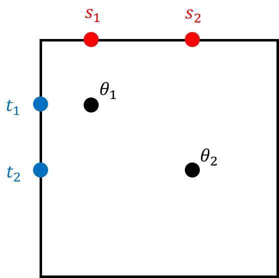
(a)

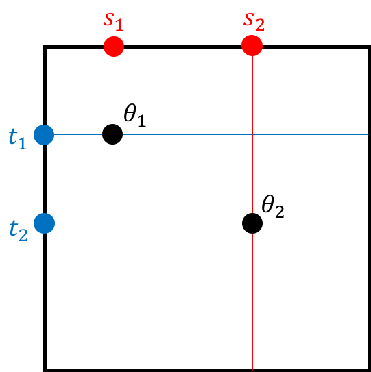
(b)

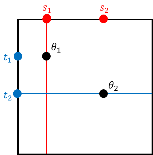
(c)

Figure 1: This figure visualizes the idea behind the proof of Proposition 2, explained in Remark 3. As an example, consider the nonnegative measure $x=a_{1}\delta_{\theta_{1}}+a_{2}\delta_{\theta_{2}}$. The locations of two impulses at $\theta_{1}=(t_{1},s_{1})\in\mathbb{I}^{2}$ and $\theta_{2}=(t_{2},s_{2})\in\mathbb{I}^{2}$ are shown with black dots in Figure 1a. For Program (5) to successfully recover $x$ from the image $y$ in (8), we should construct a nonnegative polynomial $Q$ of the form of (9) that has zeros exactly on $\theta_{1}$ and $\theta_{2}$. We do so by combining a number of univariate polynomials in $t$ and $s$. More specifically, consider a nonnegative polynomial $q_{t_{1}}(t)=\sum_{m=1}^{M}b^{11}_{m}\phi_{m}(t)$ that vanishes only at $t_{1}$. Likewise, consider similar nonnegative polynomials $q_{t_{2}}(t)$, $q_{s_{1}}(s)$, and $q_{s_{2}}(s)$, which are zero only at $t_{2}$, $s_{1}$, and $s_{2}$, respectively. Figure 1b shows the zero set of the polynomial $q_{t_{1}}(t)q_{s_{2}}(s)$ as the union of blue and red lines. Similarly, Figure 1c shows the zero set of the polynomial $q_{t_{2}}(t)q_{s_{1}}(s)$. Note that the intersection of these two zero sets is exactly $\{\theta_{1},\theta_{2}\}$. That is, $q(\theta)=q_{t_{1}}(t)q_{s_{2}}(s)+q_{t_{2}}(t)q_{s_{1}}(s)$ is a nonnegative polynomial of the form in (9) that has zeros only at $\{\theta_{1},\theta_{2}\}$, as desired. It only remains now to construct the univariate polynomials $q_{t_{1}},q_{t_{2}},q_{s_{1}},q_{s_{2}}$ described above. When the measurement functions $\{\phi_{m}\}_{m=1}^{M}$ form a $\mathcal{C}$-system and $M\geq 2K+1$, the existence of these univariate polynomials follows from standard results. We note that the construction of $Q$ in this example is slightly different from the proof of Proposition 2, in order to simplify this presentation.

2.2 Arbitrary Measure With Noise

In this section, we present the main result of this paper. Theorem 12 below generalizes Proposition 2 to account for  model mismatch, where $x$ is not necessarily a well-separated sparse measure but might be close to one, and  imaging noise ($\delta\geq 0$). That is, Theorem 12 below addresses the stability of Program (5) to model mismatch and its robustness against imaging noise. Some preparation is necessary before presenting the result.

2.2.1 Separation

Unlike sparse and noise-free super-resolution in Proposition 2, a notion of separation will play a role in Theorem 12.

Definition 4 (Separation).

For an atomic measure $x$ supported on $\Theta=\{\theta_{k}\}_{k=1}^{K}=\{(t_{k},s_{k})\}_{k=1}^{K}\subset\mathbb{I}^{2}$, let $\text{sep}(x)$ denote the minimum separation between all impulses in $x$ and the boundary of $\mathbb{I}^{2}$. That is, $\mathrm{sep}(x)$ is the largest number $\nu$ such that

$$\nu\leq\left|t_{k}-t_{l}\right|,\qquad\nu\leq\left|s_{k}-s_{l}\right|,\qquad k\neq l,\,\,k,l\in[K],$$

$$\nu\leq\left|t_{k}-0\right|,\qquad\nu\leq\left|t_{k}-1\right|,$$

$$\nu\leq\left|s_{k}-0\right|,\qquad\nu\leq\left|s_{k}-1\right|.$$ (10)

Naturally, if the measure $x$ satisfies $\text{sep}(x)=\varepsilon$, we call $x$ an $\varepsilon$-separated measure.

For example, for $x$ in Figure 1a, we have $\text{sep}(x)=\min(t_{2}-t_{1},s_{2}-s_{1},t_{1},1-t_{2},s_{1},1-s_{2})$. We remark that our notion of separation is more restrictive than the one commonly used in the super-resolution literature [12, 28, 29], as it requires the point sources to be separated in both $t$ and $s$ directions by at least $\nu$.

2.2.2 Generalized Wasserstein distance

As an error metric, we will use the generalized Wasserstein distance [30], which is closely related to the notion of unbalanced transport [31]. We first recall the total-variation (TV) norm of a measure on $\mathbb{I}^{2}$ [32] is defined as $\|z\|_{\mathrm{TV}}=\int_{\mathbb{I}^{2}}|z(\mathrm{d}t)|$, akin to $\ell_{1}$-norm in finite dimensions. Recall also that the Wasserstein distance  [32] for two nonnegative measures $z_{1}$ and $z_{2}$, supported on $\mathbb{I}^{2}$, is defined as

$$d_{\mathrm{W}}\left(z_{1},{z}_{2}\right)=\inf\int_{\mathbb{I}^{2}\times\mathbb{I}^{2}}\left\|\tau_{1}-{\tau_{2}}\right\|_{1}\cdot\gamma\left(\mathrm{d}\tau_{1},\mathrm{d}{\tau_{2}}\right),$$ (11)

where the infimum is over every nonnegative measure $\gamma$ on $\mathbb{I}^{2}\times\mathbb{I}^{2}$ that produces $z_{1}$ and ${z}_{2}$ as marginals, i.e.,

$$z_{1}(A_{1})=\int_{A_{1}\times\mathbb{I}^{2}}\gamma(\mathrm{d}\tau_{1},\mathrm{d}\tau_{2}),\qquad z_{2}(A_{2})=\int_{\mathbb{I}^{2}\times A_{2}}\gamma(\mathrm{d}\tau_{1},\mathrm{d}\tau_{2}),$$ (12)

for all measurable sets $A_{1},A_{2}\subseteq\mathbb{I}^{2}$. If we were to think of $z_{1},z_{2}$ as two piles of dirt, then $d_{\mathrm{W}}(z_{1},z_{2})$ is the least amount of work needed to transform one pile to the other. The Wasserstein distance is defined only if the TV norms of the two measures are equal, i.e., $\|z_{1}\|_{\mathrm{TV}}=\|z_{2}\|_{\mathrm{TV}}$. The generalized Wasserstein distance extends $d_{\mathrm{W}}$ and allow s for calculating the distance between nonnegative measures with different TV norms.

Definition 5 (Generalized Wasserstein distance).

For two nonnegative measures $x_{1}$ and $x_{2}$ supported on $\mathbb{I}^{2}$, their generalized Wasserstein distance is defined as

$$d_{\mathrm{GW}}\left(x_{1},x_{2}\right)=\inf\left(\left\|x_{1}-z_{1}\right\|_{\mathrm{TV}}+d_{\mathrm{W}}\left(z_{1},{z_{2}}\right)+\left\|{x_{2}}-{z_{2}}\right\|_{\mathrm{TV}}\right),$$ (13)

where the infimum is over every pair of nonnegative Borel measures $z_{1}$ and ${z}_{2}$ supported on $\mathbb{I}^{2}$ such that $\|z_{1}\|_{\mathrm{TV}}=\|{z}_{2}\|_{\mathrm{TV}}$.

Compared to (11), the two new terms in (13) gauge the difference between the mass of $x_{1}$ and the mass of $x_{2}$. Our choice of error metric $d_{\mathrm{GW}}$ is natural in the sense that any solution of Program (5) is itself a measure. However, note that controlling the error in the space of measures in our main result below does not immediately translate into controlling the error in the location of point sources, which may be estimated by, for example, applying the Prony’s method [17] to a solution of Program (5).

For instance, when $\varepsilon$ is infinitesimally small, the measure $\delta_{1/2}+\delta_{1/2+\varepsilon}$ has a small distance in the Wasserstein metric from the measure $2\delta_{1/2}$, but it is indeed impossible to distinguish the two impulses in the presence of noise in general, unless we impose additional structure on the noise. Nevertheless, in the limit of vanishing noise, it is possible to directly control the error in the location of point sources and we refer the reader to [33, 34, 35] for the details.

2.2.3 Model mismatch

Our main result, Theorem 12 below, bounds the recovery error $d_{\mathrm{GW}}(x,\widehat{x})$, where $\widehat{x}$ is a solution of Program (5). Note that, even though $x$ is an arbitrary nonnegative measure in this section, it can always be approximated with a well-separated sparse measure, up to some error with respect to the metric $d_{\mathrm{GW}}$. This sparse measure will play a key role in Theorem 12.

Definition 6 (Residual).

For a nonnegative measure $x$ supported on $\mathbb{I}^{2}$, given an integer $K$ and $\varepsilon\in(0,1/2]$, there exists a $K$-sparse nonnegative measure $x_{K,\varepsilon}$ that is $\varepsilon$-separated and well-approximates $x$. More specifically, for any $\varepsilon\in(0,1/2]$, there exists a $K$-sparse and $\varepsilon$-separated nonnegative measure $x_{K,\varepsilon}$ such that

$$R(x,K,\varepsilon):=d_{\mathrm{GW}}\left(x,x_{K,\varepsilon}\right)=\min d_{\mathrm{GW}}(x,\chi),$$ (14)

where the minimum above is over every nonnegative $K$-sparse and $\varepsilon$-separated measure $\chi$ supported on $\mbox{interior}(\mathbb{I}^{2})$.

In words, the residual $R(x,K,\varepsilon)$ can be thought of as the mismatch in modelling $x$ with a well-separated sparse measure. Indeed, note that the minimum in (14) is achieved: We can limit the search in (14) to the (bounded) set of $K$-sparse and $\varepsilon$-separated measures with TV norm bounded by $\|x\|_{\mathrm{TV}}$. This set is also closed, with respect to the weak topology imposed by $d_{\mathrm{GW}}$, see [30, Theorem 13], and thus compact. Lastly, the objective function $d_{\mathrm{GW}}$ of (14) is a norm and thus continuous a fortiori, hence the claim.

2.2.4 Smoothness

For Program (5) to succeed in the general settings of this section, we also impose additional requirements on the imaging apparatus in the next two paragraphs. We assume in this section that the imaging apparatus is smooth in the following sense.

Definition 7 (Smoothness).

The imaging apparatus in (4) is $L$-Lipschitz-continuous if

$$\left\|\int_{\mathbb{I}^{2}}\Phi(\theta)(x_{1}(\mathrm{d}\theta)-x_{2}(\mathrm{d}\theta))\right\|_{\mathrm{F}}\leq L\cdot d_{\mathrm{GW}}(x_{1},x_{2}),$$ (15)

for every pair of measures $x_{1},x_{2}$ supported on $\mathbb{I}^{2}$.

It is often not difficult to verify the Lipschitz-continuity of $\Phi$ with respect to $d_{\mathrm{GW}}$, as the following example demonstrates.

Example 8 (Smoothness).

As a toy example, suppose for simplicity that $\|x_{1}\|_{\mathrm{TV}}=\|x_{2}\|_{\mathrm{TV}}$, so that $d_{\mathrm{GW}}(x_{1},x_{2})=d_{\mathrm{W}}(x_{1},x_{2})$, see (13). Moreover, for clarity, let $m=1$ and note that

$$\int\Phi(\theta)(x_{1}(\mathrm{d}\theta)-x_{2}(\mathrm{d}\theta))=\int\phi(t)\phi(s)(x_{1}(\mathrm{d}t,\mathrm{d}s)-x_{2}(\mathrm{d}t,\mathrm{d}s)),$$ (16)

where $\phi$ is the measurement window. Let also $L_{\phi}$ denote the Lipschitz constant of $\phi(t)\phi(s)$ with respect to $\ell_{1}$-norm, i.e.,

$$\left|\phi(t_{1})\phi(s_{1})-\phi(t_{2})\phi(s_{2})\right|\leq L_{\phi}(|t_{1}-t_{2}|+|s_{1}-s_{2}|),$$ (17)

for every $t_{1},t_{2},s_{1},s_{2}\in\mathbb{I}$. Then, recalling the Kantorovich duality [32], we may write that

$$\left\|\int_{\mathbb{I}^{2}}\Phi(\theta)(x_{1}(\mathrm{d}\theta)-x_{2}(\mathrm{d}\theta))\right\|_{\mathrm{F}} =\left|\int_{\mathbb{I}}\phi(t)\phi(s)(x_{1}(\mathrm{d}t,\mathrm{d}s)-x_{2}(\mathrm{d}t,\mathrm{d}s))\right|\qquad{\color[rgb]{0,0,0}\text{(see \eqref{eq:simple1})}}$$

$$=L_{\phi}\left|\int_{\mathbb{I}}\frac{\phi(t)\phi(s)}{L_{\phi}}(x_{1}(\mathrm{d}t,\mathrm{d}s)-x_{2}(\mathrm{d}t,\mathrm{d}s))\right|$$

$$\leq L_{\phi}\cdot\max_{\psi}\int\psi(\theta)x_{1}(\mathrm{d}\theta)-\psi(\theta)x_{2}(\mathrm{d}\theta)$$

$$=L_{\phi}\cdot d_{\mathrm{W}}(x_{1},x_{2})\qquad\text{(Kantorovich duality)}$$

$$=L_{\phi}\cdot d_{\mathrm{GW}}(x_{1},x_{2}),\qquad\text{(simplifying assumption)}$$ (18)

where the maximum in the third line above is over all $1$-Lipschitz-continuous functions $\psi:\mathbb{I}^{2}\rightarrow\mathbb{R}$ with respect to $\ell_{1}$-norm. We conclude that (15) holds with $L=L_{\phi}$ in this example. $\blacksquare$

2.2.5 $\mathcal{C}^{*}$-system

To study the stability of Program (5), we also need to modify the notion of $\mathcal{C}$-system in Definition 1. We begin with the definition of an admissible sequence, visualized in Figure 2.

Definition 9 (Admissible sequence).

For a pair of integers $K$ and $M$ obeying $M\geq 2K+1$, we say that $\{\{\tau_{k}^{n}\}_{k=0}^{M}\}_{n\geq 1}\subset\mathbb{I}$ is a $(K,\varepsilon)$-admissible sequence if:

1. $\tau_{0}^{n}=0$ and $\tau_{M}^{n}=1$ for every $n$, i.e., the endpoints of $\mathbb{I}=[0,1]$ are included in the increasing sequence $\{\tau_{k}^{n}\}_{k=0}^{M}$, for every $n$.

2. As $n\rightarrow\infty$, the increasing sequence $\{\tau_{k}^{n}\}^{M-1}_{k=1}$ converges (element-wise) to an $\varepsilon$-separated finite subset of $\mathbb{I}$ with at most $K$ distinct points, where every element has an even multiplicity, except one element that appears only once.

While $\mathcal{C}$-system in Definition 1 is a condition on all increasing sequences of length $M$, the $\mathcal{C}^{*}$-system below is a condition only on admissible sequences; these are the only sequences that matter in our analysis. Like a $\mathcal{C}$-system, a $\mathcal{C}^{*}$-system imposes certain requirements on a family of functions. Whereas the performance of Program (5) for sparse measures and in the absence of noise relates to a certain $\mathcal{C}$-system in Proposition 2, the general performance of Program (5) relates to certain $\mathcal{C}^{*}$-systems, as we will see shortly in Theorem 12. The definition of $\mathcal{C}^{*}$-system below is immediately followed by its motivation.

Definition 10 ($\mathcal{C}^{*}$-system).

For an integer $K$ and an even integer $M$ obeying $M\geq 2K+2$, real-valued functions $\{\phi_{m}\}_{m=0}^{M}$ form a $\mathcal{C}^{*}_{K,\varepsilon}$-system on $\mathbb{I}$ if every $(K,\varepsilon)$-admissible sequence $\{\{\tau_{k}^{n}\}_{k=0}^{M}\}_{n\geq 1}$ satisfies:

1. The determinant of the $(M+1)\times(M+1)$ matrix $[\phi_{m}(\tau_{k}^{n})]_{k,m=0}^{M}$ is positive for all sufficiently large $n$.

2. Moreover, all minors along the $\underline{l}$th row of the matrix $[\phi_{m}(\tau_{k}^{n})]_{k,m=0}^{M}$ approach zero at the same rate when $n\rightarrow\infty$. Here, $\underline{l}$ is the index of the element of the limit sequence that appears only once.

Remark 11 (Properties of $\mathcal{C}^{*}$-systems).

Note that a $\mathcal{C}^{*}_{K,\varepsilon}$-system on $\mathbb{I}$ is also a $\mathcal{C}^{*}_{K^{\prime},\varepsilon}$-system for every integer $K^{\prime}\leq K$. Indeed, this claim follows from the observation that every $(K^{\prime},\varepsilon)$-admissible sequence is itself a $(K,\varepsilon)$-admissible sequence.  Moreover, if $\{\phi_{m}\}_{m=0}^{M}$ form a $\mathcal{C}^{*}_{K,\varepsilon}$-system on $\mathbb{I}$, then so do the scaled functions $\{c_{m}\phi_{m}\}_{m=0}^{M}$ for positive constants $\{c_{m}\}_{m=0}^{M}$.

Let us also offer some insight about $\mathcal{C}^{*}$-systems. In the proof of Proposition 2 for sparse and noise-free super-resolution, in order to construct a polynomial

$$\sum_{m=1}^{M}b_{m}\phi_{m}\geq 0,$$

with prescribed zeros on $\mathbb{I}$, we require that $\{\phi_{m}\}_{m=1}^{M}$ form a $\mathcal{C}$-system; see the discussion after Definition 1. On the other hand, for a given function $\phi_{0}$ (which, in our context, will signify the stability to noise in super-resolution), in order to construct a polynomial

$$\sum_{m=1}^{M}b_{m}\phi_{m}\geq\phi_{0},$$

where equality holds at prescribed points in $\mathbb{I}$, it is natural to require ${\color[rgb]{0,0,0}\{\phi_{0}\}}\cup\{\phi_{m}\}_{m=1}^{M}$ to form a $\mathcal{C}$-system. The definition of $\mathcal{C}^{*}$-system above is based on the same idea but limited to admissible sequences, to ease the burden of verifying the conditions in Definition 10. In particular, Definition 10 will help exclude trivial polynomials, such as $0\cdot\phi_{0}+\sum_{m=1}^{M}b_{m}\phi_{m}$.

We remark that Definition 10 only considers admissible sequences to simplify the burden of verifying whether a family of functions form a $\mathcal{C}^{*}$-system.

To summarize, the widely-used notion of $\mathcal{C}$-system in Definition 1 plays a key role in the analysis of sparse inverse problems in the absence of noise, whereas $\mathcal{C}^{*}$-system above was introduced in [1] and tailored for the stability analysis of sparse inverse problems. It was established in [1] that translated copies of the Gaussian window $e^{-t^{2}}$ indeed form a $\mathcal{C}^{*}$-system, under mild conditions reviewed in Section 2.3 below. We suspect this to also hold for many other measurement windows with sufficiently fast decay.

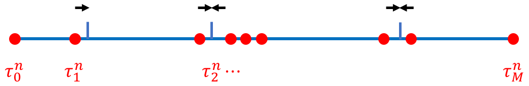
Figure 2: This figure illustrates an example of an admissible sequence; see Definition 9. For a fixed $n$, the red dots form the increasing sequence $\{\tau_{k}^{n}\}^{M}_{k=0}$. Note that the end points of the interval are included in the sequence , i.e., $\tau_{0}^{n}=0$ and $\tau^{n}_{M}=1$. In view of Definition 9, as $n\rightarrow\infty$, the sequence $\{\tau_{k}^{n}\}_{k=1}^{M-1}$ converges element-wise to three distinct points on the interior of the interval, shown with blue bars. Moreover, all limit points in $(0,1)$ have an even multiplicity except for one, which has a multiplicity of exactly one.

2.2.6 Main Result

We are now ready to present the main result of this paper, which quantifies the performance of Program (5) in the general case where $x$ is an arbitrary nonnegative measure on $\mathbb{I}^{2}$ and in the presence of additive noise. Theorem 12, proved in Section 4.4, states that Program (5) approximately recovers $x$ provided that certain $\mathcal{C}$- and $\mathcal{C}^{*}$-systems exist. As an example of this general result, Section 2.3 later specializes Theorem 12 for imaging under Gaussian blur.

Theorem 12 (Arbitrary measure with noise).

Consider a nonnegative measure $x$ supported on $\mathbb{I}^{2}$. Consider also a noise level $\delta\geq 0$, measurement functions $\{\phi_{m}\}_{m=1}^{M}$, and the image $y\in\mathbb{R}^{M\times M}$, see (3,4). We assume that the imaging apparatus is $L$-Lipschitz in the sense of (15).

For an integer $K$ and $\varepsilon\in(0,1/2]$, let $x_{K,\varepsilon}$ be a $K$-sparse and $\varepsilon$-separated nonnegative measure on $\mathbb{I}^{2}$ that approximates $x$ with the residual of $R(x,K,\varepsilon)$, in the sense of (14). In particular, let $\Theta=\{\theta_{k}\}_{k=1}^{K}=\{(t_{k},s_{k})\}_{k=1}^{K}\subset\operatorname{interior}(\mathbb{I}^{2})$ denote the support of $x_{K,\varepsilon}$, and set $T=\{t_{k}\}_{k=1}^{K}$ and $S=\{s_{k}\}_{k=1}^{K}$ for short.

With $\widehat{x}$ denoting a solution of Program (5) for $\delta^{\prime}\geq(1+L\cdot R(x,k,\varepsilon))\delta$, it holds that

$$d_{\mathrm{GW}}\left(x,\widehat{x}\right) \leq c_{1}\delta+{\color[rgb]{0,0,0}c_{2}(\varepsilon)}+c_{3}R(x,K,\varepsilon),$$ (19)

where $d_{\mathrm{GW}}$ is the generalized Wasserstein metric in (13). Above, $c_{1},c_{2}(\varepsilon),c_{3}$ are specified explicitly in (48), and depend on the the measure $x$, the separation $\varepsilon$, and the measurement functions $\{\phi_{m}\}_{m=1}^{M}$. In particular, it holds that $c_{2}(0)=0$.

The error bound in (19) holds if $M\geq 2K+2$ and

1. $\{\phi_{m}\}_{m=1}^{M}$ form a $\mathcal{C}$-system on $\mathbb{I}$,

2. $\{F_{T_{\Omega}}\}\cup\{\phi_{m}\}_{m=1}^{M}$ and $\{F_{S_{\Omega}}\}\cup\{\phi_{m}\}_{m=1}^{M}$ both form $\mathcal{C}^{*}_{K,\varepsilon}$-systems on $\mathbb{I}$ for every $\Omega\subseteq[K]$,

3. $\{F_{t_{k}}^{+}\}\cup\{\phi_{m}\}_{m=1}^{M}$ and $\{F_{t_{k}}^{-}\}\cup\{\phi_{m}\}_{m=1}^{M}$ both form $\mathcal{C}^{*}_{K,\varepsilon}$-systems on $\mathbb{I}$ for every $k\in[K]$,

4. $\{F_{s_{k}}^{+}\}\cup\{\phi_{m}\}_{m=1}^{M}$ form a $\mathcal{C}^{*}_{K,\varepsilon}$-system on $\mathbb{I}$ for every $k\in[K]$.

Above, for every index set $\Omega\subseteq[K]$ and $k\in[K]$, we define the functions $F_{T_{\Omega}},F_{S_{\Omega}},F_{t_{k}}^{\pm},F_{s_{k}}^{+}:\mathbb{I}\rightarrow\mathbb{R}$ as

$$F_{T_{\Omega}}(t):=\begin{cases}0,&\text{when there exists }k\in\Omega\text{ such that }|t-t_{k}|\leq\varepsilon/2,\\ 1,&\text{elsewhere on }\operatorname{interior}(\mathbb{I}),\end{cases}$$

$$F_{S_{\Omega}}(s):=\begin{cases}0,&\text{when there exists }k\in\Omega\text{ such that }|s-s_{k}|\leq{\varepsilon}/2,\\ 1,&\text{elsewhere on }\operatorname{interior}(\mathbb{I}),\end{cases}$$

$$F_{t_{k}}^{\pm}(t):=\begin{cases}\pm 1,&\text{when }|t-t_{k}|\leq\varepsilon/2,\\ 0,&\text{everywhere else on }\operatorname{interior}(\mathbb{I}),\end{cases}$$

$$F_{s_{k}}^{+}(s):=\begin{cases}1,&\text{when }|s-s_{k}|\leq\varepsilon/2,\\ 0,&\text{everywhere else on }\operatorname{interior}(\mathbb{I}).\end{cases}$$

An example of the functions in Theorem 12 appears in Figure 3e, where the purple graph is an example of $F_{T_{\Omega}}$ for $\Omega=\{t_{1}\}$, shown in the figure as $F_{t_{1}}$ for brevity. Theorem 12 for image super-resolution is unique in a number ways. The differences with prior work are further discussed in Section 3 and also summarized here. First, Theorem 12 applies to arbitrary measures, not only atomic ones. In particular, for atomic measures, no minimum separation or limit on the density of impulses are imposed in contrast to earlier results [2, 13, 14, 34].

Moreover, Theorem 12 addresses both noise and model-mismatch in image super-resolution. Indeed, even in the 1-D case, stability was identified as a technical obstacle in earlier work [2]. In addition, the recovery error in Theorem 12 is quantified with a natural metric between measures, i.e., the generalized Wasserstein metric, in contrast to prior work; see for example [37] that separately studies the error near and away from the impulses. Lastly, the measurement functions $\{\phi_{m}\}_{m}$ are required to be continuous rather than (several times) differentiable [2, 34]. All this is achieved without the need to explicitly regularize for sparsity in Program (5).

Note also that, in practice, we often have an upper bound for the noise level $\delta$ and the model mismatch $R(x,K,\epsilon)$, which would allow us to apply Theorem 12. This approach to quantifying stability against noise and model mismatch is common in model-based signal processing [38].

Several additional remarks are in order about Theorem 12.

Remark 13 (Proof technique).

For Program (5) to successfully recover a sparse measure in the absence of noise, we constructed a nonnegative polynomial $Q(\theta)$, within the span of the measurement functions, which vanished only at the impulse locations $\Theta=\{\theta_{k}\}_{k=1}^{K}=\{(t_{k},s_{k})\}_{k=1}^{K}$, see the discussion after Proposition 2. For approximate recovery in the presence of model mismatch and noise, we need to construct a nonnegative polynomial $Q(\theta)$ that is bounded away from zero far from the impulse locations $\Theta$, i.e.,

$$Q(\theta)\geq\overline{g}>0,\qquad{\color[rgb]{0,0,0}\text{for every }}\theta\text{ far from }\Theta,$$

where $\overline{g}$ is a positive scalar. Letting $T=\{t_{k}\}_{k=1}^{K}$ and $S=\{s_{k}\}_{k=1}^{K}$ for short, the proof of Theorem 12 constructs $Q$ by combining certain univariate polynomials, similar to the proof of Proposition 2 which was itself summarized earlier in Section 2.1 , and illustrated in Figure 1. Among these univariate polynomials, for example, the proof constructs a nonnegative polynomial $q_{T}$ such that

$$q_{T}(t)\geq 1,\qquad{\color[rgb]{0,0,0}\text{for every }}t\text{ far from }T.$$

As shown in [1], such a univariate polynomial $q_{T}$ exists if $\{F_{T}\}\cup\{\phi_{m}\}_{m=1}^{M}$ form a $\mathcal{C}^{*}$-system. In addition to $Q$, we also find it necessary to construct yet another nonnegative polynomial $Q^{0}$ to control the recovery error near the impulse locations and thus complete the proof of Theorem 12, see Section 4.4 for more details. Figure 3 illustrates some of the key ideas in the proof of Theorem 12.

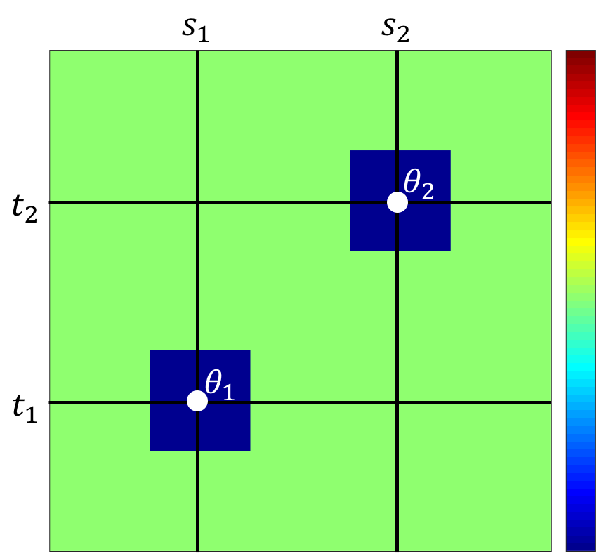
(a)

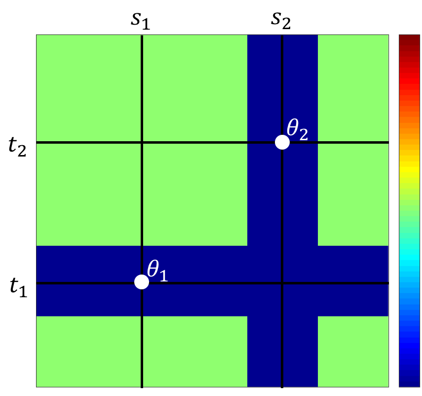
(b)

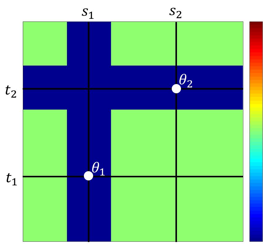
(c)

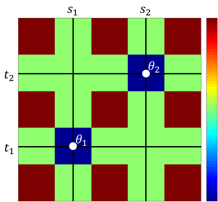
(d)

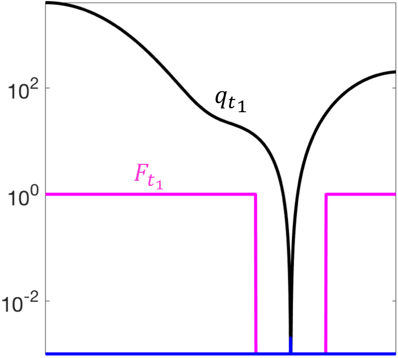
(e)

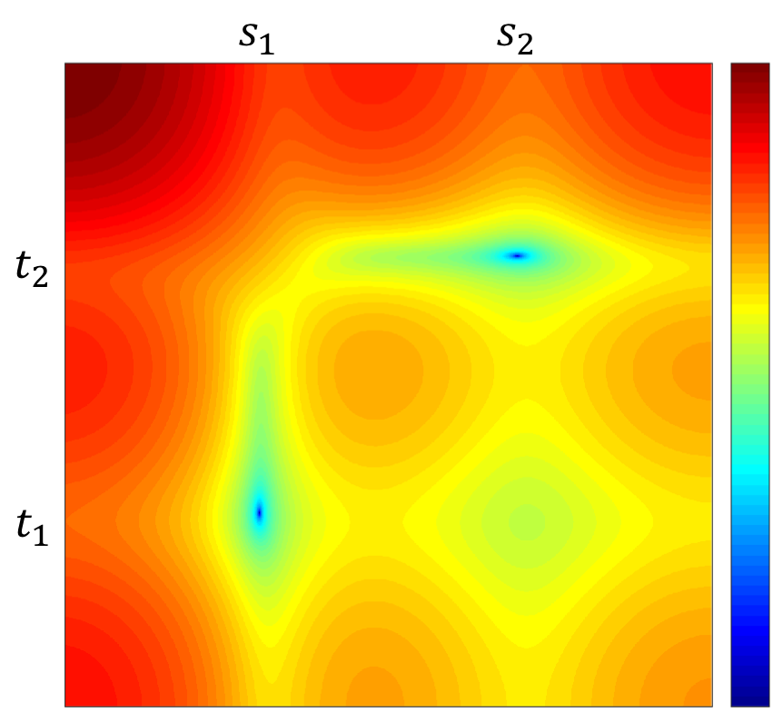
(f)

Figure 3: This figure visualizes some of the principle ideas behind the proof of Theorem 12, explained in Remark 13. As an example, consider the nonnegative measure $x=a_{1}\delta_{\theta_{1}}+a_{2}\delta_{\theta_{2}}$. The locations of two impulses at $\theta_{1}=(t_{1},s_{1})\in\mathbb{I}^{2}$ and $\theta_{2}=(t_{2},s_{2})\in\mathbb{I}^{2}$ are shown with white dots, and the black lines show the corresponding grid. For Program (5) to approximately recover $x$ from the noisy image $y$ given in (2), we need to construct a nonnegative polynomial $Q$ of the form in (9) that is zero at the impulse locations and large away from the impulses, to ensure stability. That is, we need $Q(\theta_{1})=Q(\theta_{2})=0$, and also $Q(\theta)\geq\overline{g}>0$ when $\theta$ is far from both $\theta_{1},\theta_{2}$, for a positive scalar $\overline{g}$. This lower bound for the polynomial $Q$ is shown in Figure 3a as a heat map, with warmer colors corresponding to larger values, i.e., blue corresponds to zero and green corresponds to $\overline{g}$.
Let us first express this lower bound on $Q$ in terms of univariate functions. To that end, consider a function $F_{t_{1}}(t)$ that is zero near and equal to $\sqrt{\overline{g}}$ away from $t_{1}$. Likewise, consider similar nonnegative functions $F_{t_{2}}(t),F_{s_{1}}(s),F_{s_{2}}(s)$ that are zero near and equal to $\sqrt{\overline{g}}$ away from $t_{2},s_{1},s_{2}$, respectively. Figure 3b shows the heat map of $F_{t_{1}}(t)F_{s_{2}}(s)$, Figure 3c shows the heat map of $F_{t_{2}}(t)F_{s_{1}}(s)$, and lastly Figure 3d shows the heat map of their sum, i.e., $G(\theta):=F_{t_{1}}(t)F_{s_{2}}(s)+F_{t_{2}}(t)F_{s_{1}}(s)$. Note that $G$ is zero near and larger than $\overline{g}$ away from the impulse locations $\theta_{1},\theta_{2}$, as desired.
It only remains to construct the univariate polynomials $q_{t_{1}},q_{t_{2}},q_{s_{1}},q_{s_{2}}\in\text{span}(\phi_{1},\cdots,\phi_{M})$ that satisfy the inequalities $q_{t_{1}}\geq F_{t_{1}}$, $q_{t_{2}}\geq F_{t_{2}}$, $q_{s_{1}}\geq F_{s_{1}}$, $q_{s_{1}}\geq F_{s_{1}}$, with equality at $t_{1},t_{2},s_{1},s_{2}$, respectively. Under the assumptions of Theorem 12, the existence of these univariate polynomials follows from [1]. In this fashion, we finally obtain a nonnegative polynomial $Q(\theta)=q_{t_{1}}(t)q_{s_{2}}(s)+q_{t_{2}}(t)q_{s_{1}}(s)$ that is zero at the impulse locations and larger than $\overline{g}$ away from the impulses, as desired. For example, for the Gaussian window detailed in Section 2.3 with the standard deviation $\sigma=0.2$, Figure 3e shows $q_{t_{1}}(t)$ and Figure 3f shows the heat map of the dual certificate $Q(\theta)$, both in logarithmic scale. Yet, another polynomial $Q^{0}$ is needed to control the recovery error near the impulses and thus complete the proof of Theorem 12, see Section 4.4.

Remark 14 (Recovery error).

The bound on the recovery error $d_{\mathrm{GW}}(x,\widehat{x})$ in (19) depends on the noise level $\delta$ and on how well $x$ can be approximated with a well-separated sparse measure. More specifically, for any $\varepsilon\in(0,1/2]$, $x$ can be approximated with a $K$-sparse and $\varepsilon$-separated measure $x_{K,\varepsilon}$, with the residual of $R(x,K,\varepsilon)$, see (14). We might then think of a solution $\widehat{x}$ of Program (5) as an estimate for $x_{K,\varepsilon}$ and therefore an estimate for $x$, up to the residual $R(x,K,\varepsilon)$. Both the separation $\varepsilon$ and the residual $R(x,K,\varepsilon)$ appear on the right-hand side of the error bound (19).

In particular, when $\delta=\varepsilon=R(x,K,\varepsilon)=0$, we again obtain Proposition 2 for recovery of a $K$-sparse nonnegative measure in the absence of noise. Note that, given a noise level $\delta$, this work does not address the challenging problem of choosing the separation $\varepsilon$ in order to minimize the right-hand side of (19). Intuitively, for large $\delta$, we must choose the separation $\varepsilon$ large enough to maintain stability against the large noise level. In turn, a large $\varepsilon$ leads to a large residual $R(x,K,\varepsilon)$, see (14). The correct balance between $\epsilon$ and $R(x,K,\epsilon)$ depends on the particular choice of the measurement functions $\{\phi_{m}\}_{m}$ and is beyond the scope of this paper.

Remark 15 (Minimum separation).

Theorem 12 applies to any nonnegative measure $x$. In particular, when $x$ is an atomic measure, Theorem 12 applies regardless of the separation between the impulses present in the measure $x$. However, it is crucial to note that the recovery error $d_{\mathrm{GW}}(x,\widehat{x})$ does indeed depend on the separation of $x$.

As an example, consider the atomic measure $x=\delta_{0.5}+\delta_{0.51}$. In order to apply Theorem 12, we can set $\varepsilon=0.01$, so that $x_{K,\varepsilon}=x$ and $R(x,K,\varepsilon)=0$. Now, the error bound in (19) reads as

$$d_{\mathrm{GW}}(x,\widehat{x})\leq{\color[rgb]{0,0,0}c_{1}(0.01)\cdot\delta+c_{2}(0.01)},$$ (20)

where we have made explicit the dependence of $c_{1}$ on $\varepsilon$ for emphasis. Alternatively, we may also apply Theorem 12 by setting $\varepsilon=0.2$, so that $x_{K,\varepsilon}=\delta_{0.405}+\delta_{0.605}$ and $R(x,K,\varepsilon)=0.19$. In this case, (19) reads as

$$d_{\mathrm{GW}}(x,\widehat{x})\leq{\color[rgb]{0,0,0}c_{1}(0.2)\cdot\delta+c_{2}(0.2)+c_{3}(\varepsilon)\cdot 0.19.}$$ (21)

This work, however, does not address the optimal choice of separation $\varepsilon$ as a function of noise level $\delta$. That is, given $\delta$, the choice of $\varepsilon$ that would minimize the right-hand of (19) is not studied here ; see also [1].

2.3 Example with Gaussian Window

As an example of the general super-resolution framework presented in this paper, consider the case where $x$ is a $K$-sparse nonnegative measure as in (7) and $\{\phi_{m}\}_{m=1}^{M}$ are translated copies of a one-dimensional Gaussian window, i.e.,

$$\phi_{m}(t)=g_{1}(t-t^{\prime}_{m}):=e^{-(t-t^{\prime}_{m})^{2}/\sigma^{2}},$$ (22)

for $T^{\prime}=\{t^{\prime}_{m}\}_{m=1}^{M}\subset\mathbb{I}$ and standard deviation $\sigma>0$. Recalling (2), note that

$$\int_{\mathbb{I}^{2}}\phi_{m}(t)\phi_{n}(s)x(\mathrm{d}t,\mathrm{d}s) =\sum_{k=1}^{K}a_{k}\cdot g_{1}(t_{k}-t^{\prime}_{m})g_{1}(t_{k}-t^{\prime}_{n})\qquad\text{(see \eqref{eq:gauss window})}$$

$$=\sum_{k=1}^{K}a_{k}\cdot g_{2}(\theta_{k}-\theta^{\prime}_{m,n})$$

$$=\sum_{k=1}^{K}a_{k}\cdot e^{-\frac{\|\theta_{k}-\theta^{\prime}_{m,n}\|_{2}^{2}}{\sigma^{2}}},$$ (23)

where $\theta_{k}=(t_{k},s_{k}),\theta^{\prime}_{m,n}=(t^{\prime}_{m},t^{\prime}_{n})$ and $g_{2}$ is a 2-D Gaussian window, which can be thought of as the point-spread function of the imaging device. Note that we might also think of $\{\theta^{\prime}_{m,n}\}_{m,n=1}^{M}=T^{\prime}\times T^{\prime}$ as the sampling points in the sense that

$$\int_{\mathbb{I}^{2}}\phi_{m}(t)\phi_{n}(s)x(\mathrm{d}t,\mathrm{d}s)=\sum_{k=1}^{K}a_{k}\cdot g_{2}(\theta_{k}-\theta^{\prime}_{m,n})=(g_{2}\star x)(\theta^{\prime}_{m,n}),\qquad m,n\in[M],$$ (24)

where $\star$ stands for convolution. Put differently, the integral above evaluates the Gaussian-blurred (or filtered) copy of measure $x$ at locations $T^{\prime}\times T^{\prime}$.

Suppose first that there is no imaging noise and, consequently, $y_{m,n}=(g_{2}\star x)(\theta^{\prime}_{m,n})$ is the $(m,n)^{\text{th}}$ pixel of the image, for every $m,n\in[M]$. The Gaussian windows $\{\phi_{m}\}_{m=1}^{M}$, specified in (22), form a $\mathcal{C}$-system on $\mathbb{I}$ for arbitrary $T^{\prime}\subset\mathbb{I}$, see for instance [24, Example 5]. Therefore, in view of Proposition 2, the measure $x$ is the unique solution of Program (5) with $\delta^{\prime}=0$, provided that $M\geq 2K+1$. This simple argument should be contrasted with the elaborate proofs of earlier 1-D results, for example Theorem 1.3 in [2].

In the presence of noise, i.e., when $\delta\geq 0$, Lemma 23 in [1] establishes that all the families of functions in Theorem 12 are indeed $\mathcal{C}^{*}_{K,\varepsilon}$-systems on $\mathbb{I}$, provided that the endpoints of $\mathbb{I}$ are included in the sampling points $T^{\prime}$. In fact, Section 1.2 in [1] goes further and also evaluates the factors involved in the error bound for 1-D super-resolution, although arguably the result is suboptimal and there is room for improvement. In principle, those results could be in turn used to evaluate $c_{1},c_{2},c_{3}$ in the error bound of Theorem 12, a direction which is not pursued here. The conclusion of this section is recorded below.

Corollary 16 (Gaussian window).

Consider a nonnegative measure $x$ supported on $\mathbb{I}^{2}$. Consider also a noise level $\delta\geq 0$ and the family of measurement functions defined in (22). For an integer $K$ and $\varepsilon\in(0,1/2]$, let $x_{K,\varepsilon}$ be a $K$-sparse and $\varepsilon$-separated nonnegative measure on $\mathbb{I}^{2}$ that approximates $x$ in the sense of (14). With $M\geq 2K+2$, let $\widehat{x}$ be a solution of Program (5) with

$$\delta^{\prime}\geq\left(1+\sqrt{\frac{2M}{\sigma^{2}e}}R(x,k,\varepsilon)\right)\delta,$$

see (14). Then,

$$d_{\mathrm{GW}}\left(x,\widehat{x}\right) \leq c_{1}\delta+{\color[rgb]{0,0,0}c_{2}(\varepsilon)}+c_{3}R(x,K,\varepsilon),$$ (25)

where $d_{\mathrm{GW}}$ is the generalized Wasserstein metric in (13). Above, $c_{1},c_{2}(\varepsilon),c_{3}$ are specified explicitly in (48), and depend on the true measure $x$, the separation $\varepsilon$, and the sampling locations $T^{\prime}=\{t^{\prime}_{m}\}_{m=1}^{M}$ in (22). In particular, it holds that $c_{2}(0)=0$.

3 Related Work

The current wave of super-resolution research using convex optimization began with the two seminal papers of Candès and Fernandez- Granda [12, 27]. In those papers, the authors showed that a convex program with a sparse-promoting regularizer stably recovers a complex atomic measure from the low-end of its spectrum. This holds true if the minimal separation between any two spikes is inversely proportional to the maximal measured frequency, i.e., the “bandwidth” of the sensing mechanism. Many papers extended this fundamental result to randomized models [29], support recovery analysis [39, 40, 41, 37, 42], denoising schemes [43, 44], different geometries [45, 46, 47, 48, 49], and incorporating prior information [50]. Most of these works easily generalize to multi-dimensional signals. In addition, a special attention to multi-dimensional signals was given in a variety of papers; see for instance [51, 52].

The separation condition above is unnecessary for nonnegative measures, and this is the important regime on which this paper and most of this review focuses. There are a number of works that study nonnegative sparse super-resolution for atomic measures supported on a grid. In [14, 13], it was shown that for such 1-D or 2-D signals, stable reconstruction is possible without imposing a separation condition, but instead requiring a milder condition on the density of the impulses. In particular, the error grows exponentially fast as the density of the spikes increases. A similar result was derived for signals on the sphere [53].

In this paper, we focus on the grid-free setting  [54, 55] in which the nonnegative measure is not necessarily supported on a predefined grid. This is the most general regime and requires more advanced machinery and algorithms. In [2], it was shown that in the absence of noise, a convex program with TV regularizer can recover–without imposing any separation–an atomic measure on the real line [2]. The same holds on other geometries as well [45, Section 5]. However, all these results have no stability guarantees, assume a differentiable point spread function and make use of a TV regularizer to promote sparsity. Our Proposition 2 and Theorem 12 address all these shortcomings and solve the sparse (grid-free) image super-resolution problem in its most general form. The leap from the 1-D results of [1] to 2-D requires new techniques since the key technical ingredient, i.e., $\mathcal{C}$-systems, does not naturally extend to higher dimensions.

Let us add that the low-noise regime for positive 1-D super-resolution was studied in [20]. There, it was shown that a convex program with a sparse-promoting regularizer results in the same number of spikes as the original measure when the noise level is small. Furthermore, the solution converges to the underlying positive measure if the signal-to-noise ratio scales like $\mathcal{O}(1/\text{sep}^{2})$, where sep is the minimal separation between adjacent spikes. In contrast to our work, the framework of [20] builds upon smooth convolution kernel and uses a sparse-promoting regularizer, rather the feasibility problem considered in Program (5). In [33], it was shown that the 2-D version of the same program enjoys similar properties for a pair of spikes.

Going back to signed measures, another line of work is based on various generalizations of Prony’s method [56], which encodes the support of the measure as zeros of a designed polynomial. Such generalizations include methods like MUSIC [57], Matrix Pencil [18], ESPRIT [58], to name a few. In 1-D and in the absence of noise, these methods are guaranteed to achieve exact recovery for a complex measure without enforcing any separation. This is not true for convex programs in which separation is a necessary condition, see [59]. The separation is not necessary for convex programs only for nonnegative measures, like the model considered in this paper. Stability analysis of some of these methods, under a separation condition, is found in [60, 61, 62, 63, 64, 65]. However, their extension to 2-D is not trivial and accordingly different methods were proposed [66, 67, 68, 69, 70]. To the best of our knowledge, the stability of these algorithms for two or higher dimensions is not understood. That being said, we do not claim that convex programs are numerically superior over the Prony-like techniques and we leave comprehensive numerical study for future research.

4 Theory

4.1 Notation

At the risk of being redundant, let us collect here some of the notation used throughout this paper. For positive $\varepsilon$ and $T=\{t_{k}\}_{k=1}^{K}\subset\mathbb{I}$, let us define the neighbourhoods

$$t_{k,\varepsilon}:=\{t\in\mathbb{I}:|t-t_{k}|\leq\varepsilon\}\subset\mathbb{I},$$

$$T_{\varepsilon}:=\bigcup_{k=1}^{K}t_{k,\varepsilon},$$ (26)

and let $t_{k,\varepsilon}^{C}$ and $T_{\varepsilon}^{C}$ be the complements of these sets with respect to $\mathbb{I}$. Let also $\mbox{sep}(T)$ denote the minimum separation of $T$, i.e., the largest number $\nu$ for which

$$\nu\leq|t_{k}-t_{l}|,\qquad k\neq l,\,\,k,l\in[K],$$

$$\nu\leq|t_{k}-0|,\qquad\nu\leq|t_{k}-1|.$$ (27)

Likewise, for positive $\varepsilon$ and $\Theta\subset\{\theta_{k}\}_{k=1}^{K}=\{(t_{k},s_{k})\}_{k=1}^{K}\subset\mathbb{I}^{2}$, we define the neighbourhoods

$$\theta_{k,\varepsilon}:=t_{k,\varepsilon}\times s_{k,\varepsilon}=\{\theta\in\mathbb{I}^{2}:\|\theta-\theta_{k}\|_{\infty}\leq\varepsilon\}\subset\mathbb{I}^{2},$$

$$\Theta_{\varepsilon}:=\bigcup_{k=1}^{K}\theta_{k,\varepsilon}\subseteq T_{\varepsilon}\times S_{\varepsilon},$$ (28)

and let $\theta_{k,\varepsilon}^{C}$ and $\Theta_{\varepsilon}^{C}$ be the complements of these sets with respect to $\mathbb{I}^{2}$. Above, $\|\theta\|_{\infty}=\max[|t|,|s|]$ is the $\ell_{\infty}$-norm of $\theta=(t,s)$. Similarly, define the minimum separation of $\Theta$, i.e., the smallest number $\nu$ for which both (27) holds and

$$\nu\leq|s_{k}-s_{l}|,\qquad k\neq l,\,\,k,l\in[K],$$

$$\nu\leq|s_{k}-0|,\qquad\nu\leq|s_{k}-1|.$$ (29)

4.2 Proof of Proposition 2 (Sparse Measure Without Noise)

The following standard result is an immediate extension of [1, Lemma 9] and, roughly speaking, states that Program (5) is successful if a certain dual certificate $Q$ exist.

Lemma 17.

Let $x$ be a $K$-sparse nonnegative atomic measure supported on $\Theta\subset\operatorname{interior}(\mathbb{I}^{2})$, see (7). Then $x$ is the unique solution of Program (5) with $\delta^{\prime}=0$ if

• the $M^{2}\times K$ matrix $\left[\phi_{m}(t_{k})\phi_{n}(s_{k})\right]_{m,n,k=1}^{m=M,n=M,k=K}$ has full column rank, and

• there exist real coefficients $\{b_{m,n}\}_{m,n=1}^{M}$ and polynomial $Q(t,s)=\sum_{m,n=1}^{M}b_{m,n}\phi_{m}(t)\phi_{n}(s)$ such that $Q$ is nonnegative on $\operatorname{interior}(\mathbb{I}^{2})$ and vanishes only on $\Theta$.

The following result, proved in Appendix A, states that the dual certificate required in Lemma 17 exists if the number of measurements $M$ is large enough and the measurement functions $\{\phi_{m}\}_{m=1}^{M}$ form a $\mathcal{C}$-system on $\mathbb{I}$.

Lemma 18 (Sparse measure without noise).

Let $x$ be a $K$-sparse nonnegative atomic measure supported on $\operatorname{interior}(\mathbb{I}^{2})$. For $M\geq 2K+1$, suppose that $\{\phi_{m}\}_{m=1}^{M}$ form a $\mathcal{C}$-system on $\mathbb{I}$. Then, the dual certificate $Q$ prescribed in Lemma 17 exists.

Combining Lemmas 17 and 18 completes the proof of Proposition 2.

Remark 19 (Proof technique of Lemma 18).

The technical challenge in the proof of Lemma 18 is that $\mathcal{C}$-systems do not generalize to two dimensions. Indeed, to prove our claim, we effectively reduce the construction of the dual polynomial $Q(\theta)$ with $\theta=(t,s)$ into the construction of a number of univariate polynomials in $t$ and $s$. The key observation of the proof is the following. Suppose for simplicity that $\phi_{1}\equiv 1$. Recall that $\Theta=\{\theta_{k}\}_{k=1}^{K}=\{(t_{k},s_{k})\}_{k=1}^{K}$ are the impulse locations and let $T=\{t_{k}\}_{k=1}^{K}$, $S=\{s_{k}\}_{k=1}^{K}$ for short, so that $\Theta\subseteq(T\times S)$. Suppose that a univariate polynomial $q_{T}(t)$ of $\{\phi_{m}(t)\}_{m=1}^{M}$ is nonnegative on $\mathbb{I}$ and only vanishes on $T$. Similarly, consider a polynomial $q_{S}(s)$ of $\{\phi_{n}(s)\}_{n=1}^{M}$ that is nonnegative on $\mathbb{I}$ and only vanishes on $S$. Then, the polynomial $Q(\theta)=q_{T}(t)+q_{S}(s)$ is nonnegative on $\mathbb{I}^{2}$ and vanishes only on $T\times S$.

In general $\Theta\subset(T\times S)$ and, consequently, the above $Q$ will have unwanted zeros on $(T\times S)\backslash\Theta$. This issue may be addressed by replacing the $M^{2}\times K$ matrix in Lemma 17 with a larger matrix of size $M^{2}\times K^{2}$. Alternatively, we use in the proof a more nuanced argument to construct a different polynomial $Q$ that vanishes exactly on $\Theta$, without the unwanted zeros on $(T\times S)\backslash\Theta$, see Appendix A for the details. This more nuanced argument also lends itself naturally to noisy super-resolution, as we will see later.

4.3 Geometric Intuition for Proposition 2

Proposition 2 states that the imaging operator $\Phi$ in (4) is injective on all $K$-sparse nonnegative measures (such as $x$) provided that we take enough observations ($M\geq 2K+1$) and the measurement functions $\{\phi_{m}\}_{m=1}^{M}$ form a $\mathcal{C}$-system on $\mathbb{I}$. Here, we provide some geometric intuition about the role of the dual certificate in the proof of Proposition 2.

Let us denote $\theta=(t,s)$ for short and consider the closure of the conic hull of the dictionary $\{\Phi(\theta)\}_{\theta\in\mathbb{I}^{2}}$ defined as

$$\mathcal{C}:=\left\{\int_{\mathbb{I}^{2}}\Phi(\theta)\chi(d\theta)\,:\,\chi\mbox{ is a nonnegative measure on }\mathbb{I}^{2}\right\}\subset\mathbb{R}^{M\times M}.$$ (30)

By the continuity of $\Phi$ and with an application of the dominated convergence theorem, it is easy to verify that $\mathcal{C}$ is a closed convex cone, i.e., $\mathcal{C}$ is a homogeneous and closed convex subset of $\mathbb{R}^{M\times M}$. When $\{\phi_{m}\}_{m=1}^{M}$ form a $\mathcal{C}$-system on $\mathbb{I}$, it also not difficult to verify that $\{\Phi(t_{l},s_{l})\}_{l=1}^{M^{2}}$ are linearly independent matrices in $\mathbb{R}^{M\times M}$. This in particular implies that $\mathcal{C}$ is a convex body, i.e., the interior of $\mathcal{C}$ is not empty. Note also that $y\in\mathcal{C}$ because

$$y=\int_{\mathbb{I}^{2}}\Phi(\theta)x(d\theta)=\sum_{k=1}^{M}a_{k}\Phi(\theta_{k}).$$ (31)

For Program (5) to successfully recover the measure $x$, it suffices that

$$\mathcal{A}=\mbox{cone}\left(\{\Phi(\theta_{k})\}_{k=1}^{K}\right)=\left\{\sum_{k=1}^{K}\alpha_{k}\Phi(\theta_{k})\,:\,\alpha_{k}\geq 0,\,\forall k\in[K]\right\},$$ (32)

is a $K$-dimensional exposed face of the cone $\mathcal{C}$. See [71, §18] for the definition of exposed face. This in turn happens if and only if we can find a hyperplane with normal vector $b\in\mathbb{R}^{M\times M}$ that strictly supports the cone $\mathcal{C}$ at $\mathcal{A}$, i.e., when we can find $b$ such that

$$\begin{cases}\left\langle b,c\right\rangle=0,&\forall c\in\mathcal{A},\\ \left\langle b,c\right\rangle>0,&\forall c\in\mathcal{C}\backslash\mathcal{A}.\end{cases}$$ (33)

Invoking (32), we find that (33) is equivalent to finding $b\in\mathbb{R}^{M\times M}$ such that

$$\begin{cases}\left\langle b,\Phi(\theta_{k})\right\rangle=0,&k\in[K],\\ \left\langle b,\Phi(\theta)\right\rangle>0,&\theta\notin\{\theta_{k}\}_{k=1}^{K}.\end{cases}$$ (34)

In other words, for Program (5) to successfully recover the measure $x$, it suffices to find a “polynomial”

$$Q(\theta)=Q(t,s):=\langle b,\Phi(\theta)\rangle=\sum_{m,n=1}^{M}b_{m,n}\phi_{m}(t)\phi_{n}(s),$$

that vanishes on $\{\theta_{k}\}_{k=1}^{K}$ and is positive elsewhere on $\mathbb{I}^{2}$. Building on the results in [1], we construct one such polynomial in Section 4.2 when $M\geq 2K+1$. It is worth noting that the polar of the cone $\mathcal{C}$, itself another convex cone in $\mathbb{R}^{M\times M}$, consists of the coefficients of all nonnegative polynomials of $\{\phi_{m}\phi_{n}\}_{m,n=1}^{M}$ on $\mathbb{I}^{2}$ and in particular the coefficient vector $b$ above belongs to an $(M^{2}-K)$-dimensional face of this polar cone [24]. We refer the reader to Figure 4 for an illustration of the convex geometry underlying the problem of nonnegative super-resolution.

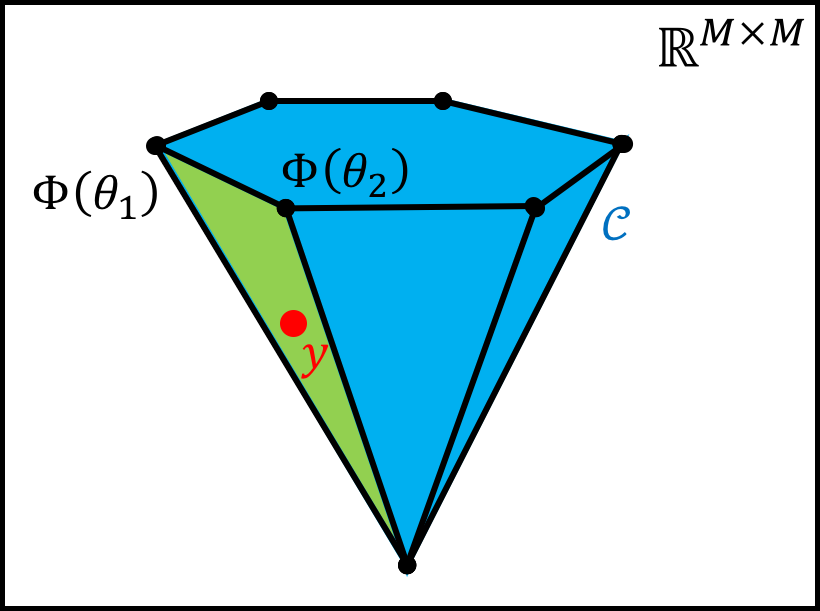
(a)

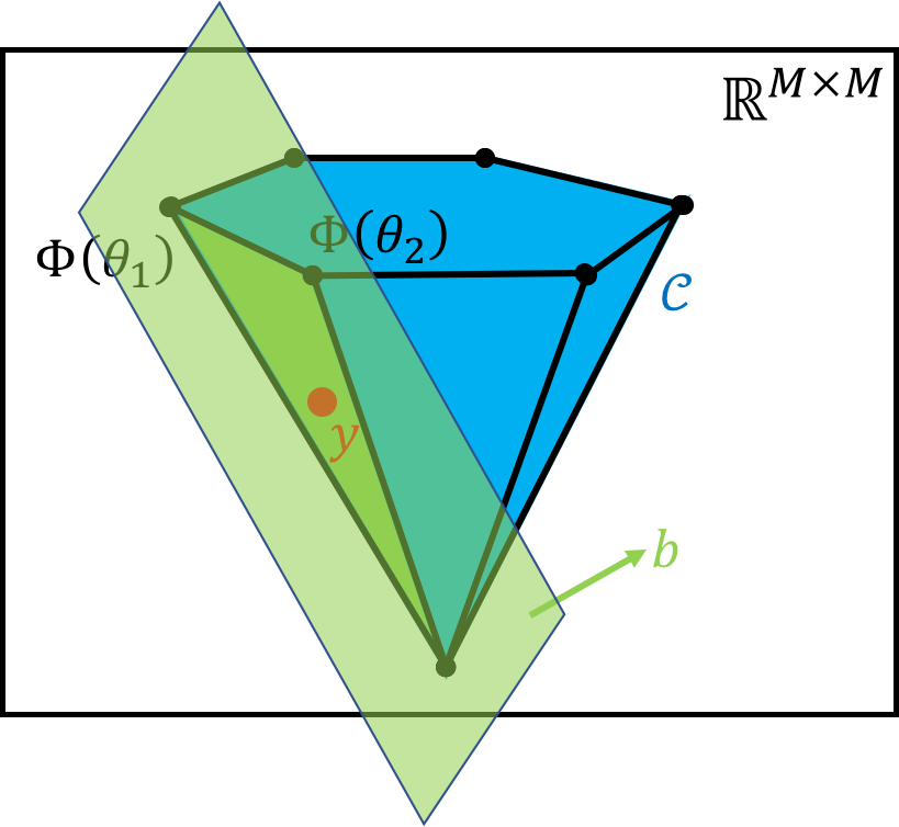
(b)

Figure 4: This figure complements Section 4.3. Figure 4a shows the conic hull $\mathcal{C}$ of the range of the imaging operator $\Phi:\mathbb{I}^{2}\rightarrow\mathbb{R}^{M\times M}$. Note that the image $y$ in (8) belongs to the cone $\mathcal{C}$, see (31). For Program (5) to successfully recover the true measure $x$ from the image $y$, it suffices that $\{\Phi(\theta_{k})\}_{k=1}^{K}$ form a $K$-dimensional exposed face of the cone $\mathcal{C}$, where $\{\theta_{k}\}_{k=1}^{K}$ is the support of the measure $x$. This face is shown in green. In words, this condition is sufficient for $x$ to be the unique solution of Program (5). Equivalently, it suffices to find a hyperplane, with normal vector $b$, that strictly supports $\mathcal{C}$ on this face. This latter condition can be interpreted as finding a nonnegative polynomial of $\{\phi_{m}(t)\phi_{n}(s)\}_{m,n=1}^{M}$ with zeros exactly on the support of the measure $x$.

4.4 Proof of Theorem 12 (Arbitrary Measure with Noise)

In this section, we will prove the main result of this paper, i.e., Theorem 12. For an integer $K$ and $\varepsilon\in(0,1/2]$, let $x_{K,\varepsilon}$ be a $K$-sparse and $\varepsilon$-separated nonnegative measure on $\mathbb{I}^{2}$ that approximates $x$ with residual $R(x,K,\varepsilon)$, in the sense of (14). Let $\Theta=\{\theta_{k}\}_{k=1}^{K}=\{(t_{k},s_{k})\}_{k=1}^{K}\subset\operatorname{interior}(\mathbb{I})^{2}$ be the support of $x_{K,\varepsilon}$, and set $T=\{t_{k}\}_{k=1}^{K}$ and $S=\{s_{k}\}_{k=1}^{K}$ for short. Consider also the neighbourhoods $\{\theta_{k,\varepsilon}\}_{k=1}^{K}\subseteq\mathbb{I}^{2}$ and $\Theta_{\varepsilon}=\cup_{k=1}^{K}\theta_{k,\varepsilon}$ defined in (28). Let $\{\theta_{k,\varepsilon}^{C}\}_{k=1}^{K}$ and $\Theta_{\varepsilon}^{C}$ denote the complements of these sets with respect to $\mathbb{I}^{2}$.

Before turning to the details, let us outline the proof. We will show in Section 4.4.1 that the existence of certain dual certificates leads to a stable recovery of $x_{K,\varepsilon}$ with Program (5). Then, we show in Section 4.4.2 that these certificates exist under certain conditions on the imaging apparatus. Finally, in Section 4.4.3, we complete the proof of Theorem 12 by applying the triangle inequality to control $d_{\mathrm{GW}}(x,\widehat{x})$ as

$$d_{\mathrm{GW}}(x,\widehat{x})\leq d_{\mathrm{GW}}(x,x_{K,\varepsilon})+d_{\mathrm{GW}}(x_{K,\varepsilon},\widehat{x})\leq R(x,K,\varepsilon)+d_{\mathrm{GW}}(x_{K,\varepsilon},\widehat{x}).\qquad\mbox{(see \eqref{eq:residual})}$$

4.4.1 Dual Certificates

Lemmas 20 and 21 below show that Program (5) stably recovers the atomic measure $x_{K,\varepsilon}$ in the presence of noise, provided that certain dual certificates exist. The proofs, which appear in Appendices B and C, are standard and Lemmas 20 and 21 below are extensions of, respectively, Lemmas  16 and 17 in [1]. In particular, Lemma 20 below controls the recovery error away from the support $\Theta$ of $x_{K,\varepsilon}$, whereas Lemma 21 controls the error near the support. The latter features an approximate dual certificate, and shares some broad similarities with [72].

Lemma 20 ( Error away from the support).

Let $\widehat{x}$ be a solution of Program (5) with $\delta^{\prime}\geq\delta$ and set $h:=\widehat{x}-x_{K,\varepsilon}$ to be the error. Fix a positive scalar $\bar{g}$. Suppose that there exist real coefficients $\{b_{m,n}\}_{m,n=1}^{M}$ and a polynomial

$$Q(\theta)=Q(t,s)=\sum_{m,n=1}^{M}b_{m,n}\phi_{m}(t)\phi_{n}(s),$$ (35)

such that

$$Q(\theta)\geq G(\theta):=\begin{cases}0,&\text{when there exists }k\in[K]\text{ such that }\theta\in\theta_{k,{\varepsilon}},\\ \bar{g},&\text{elsewhere {\color[rgb]{0,0,0} in} }\operatorname{interior}(\mathbb{I}^{2}),\end{cases}$$ (36)

where the equality holds on $\Theta=\{\theta_{k}\}_{k=1}^{K}$. Then it holds that

$$\int_{\Theta_{\varepsilon}^{C}}h(d\theta)\leq 2\|b\|_{\mathrm{F}}\delta^{\prime}/\bar{g},$$ (37)

where $b\in\mathbb{R}^{M\times M}$ is the matrix formed by the coefficients $\{b_{m,n}\}_{m,n=1}^{M}$.

Lemma 21 ( Error near the support).

Let $\widehat{x}$ be a solution of Program (5) with $\delta^{\prime}\geq\delta$ and set $h:=\widehat{x}-x_{K,\varepsilon}$ to be the error. For $\alpha\in[0,1]$, suppose that there exist real coefficients $\{b^{0}_{m,n}\}_{m,n=1}^{M}$ and a polynomial

$$Q^{0}(\theta)=Q^{0}(t,s)=\sum_{m,n=1}^{M}b_{m,n}^{0}\phi_{m}(t)\phi_{n}(s),$$ (38)

such that

$$Q^{0}(\theta)\geq G^{0}(\theta):=\begin{cases}1,&\text{when there exists }k\in[K]\text{ such that }\theta\in\theta_{k,{\varepsilon}}\text{ and }\int_{\theta_{k,{\varepsilon}}}h(d\theta)>0,\\ -1,&\text{when there exists }k\in[K]\text{ such that }\theta\in\theta_{k,{\varepsilon}}\text{ and }\int_{\theta_{k,{\varepsilon}}}h(d\theta)\leq 0,\\ {\color[rgb]{0,0,0}-1+\alpha}&{\color[rgb]{0,0,0}\text{when there exists }}{\color[rgb]{0,0,0}k\in[K]}\text{ such that }\theta=\theta_{k}\text{ and }\int_{\theta_{k,{\varepsilon}}}h(d\theta)\leq 0,\\ {\color[rgb]{0,0,0}-1},&\text{elsewhere in }\operatorname{interior}(\mathbb{I}^{2}),\end{cases}$$ (39)

where the equality holds on $\Theta$. Then it holds that

$$\sum_{k=1}^{K}\left|\int_{\theta_{k,{\varepsilon}}}h(d\theta)\right|\leq\alpha\|x_{K,\varepsilon}\|_{\mathrm{TV}}+2\left(\|b^{0}\|_{\mathrm{F}}+\frac{\|b\|_{\mathrm{F}}}{\overline{g}}\right)\delta^{\prime},$$ (40)

where $b^{0}\in\mathbb{R}^{M\times M}$ is the matrix formed by the coefficients $\{b_{m,n}^{0}\}_{m,n=1}^{M}$, and the matrix $b$ was introduced in Lemma 20.

By combining Lemmas 20 and 21, the next result bounds the error $d_{\mathrm{GW}}(x_{K,\varepsilon},\widehat{x})$. The proof is omitted as the steps are identical to those taken in Lemma 18 in [1].

Lemma 22 (Error in Wassertein metric).

Suppose that the dual certificates $Q$ and $Q^{0}$ in Lemmas 20 and 21 exist. Then,

$$d_{\mathrm{GW}}\left(x_{K,\varepsilon},\widehat{x}\right)\leq\left({\color[rgb]{0,0,0}\frac{8\|b\|_{\mathrm{F}}}{\bar{g}}}+6\|b^{0}\|_{\mathrm{F}}\right)\delta^{\prime}+{\color[rgb]{0,0,0}\left(\varepsilon+3\alpha\right)}\|x_{K,\varepsilon}\|_{\mathrm{TV}}.$$ (41)

In order to apply Lemma 22, we must first show that the dual certificates $Q$ and $Q^{0}$ specified in Lemmas 20 and 21 exist. In the next section, we construct these certificates under certain conditions on the imaging apparatus.

4.4.2 Existence of the Dual Certificates

To construct the dual certificates required in Lemmas 20 and 21, some preparation is necessary. For notational convenience, throughout we model $x_{K,\varepsilon}$ by (7), with $x$ therein replaced with $x_{K,\varepsilon}$. Then recall from Section 4.1 that $\Theta=\{\theta_{k}\}_{k=1}^{K}=\{(t_{k},s_{k})\}_{k=1}^{K}$ are the impulse locations of $x_{K,\varepsilon}$ and let $T=\{t_{k}\}_{k=1}^{K}$ and $S=\{s_{k}\}_{k=1}^{K}$ for short. In particular, note that $\Theta\subseteq T\times S$.

For an index set $\Omega\subseteq[K]$ and its complement $[K]\backslash\Omega$, we set $T_{\Omega}=\{t_{k}\}_{k\in\Omega}$ and $S_{[K]\backslash\Omega}=\{s_{k}\}_{k\in[K]\backslash\Omega}$ for brevity. For a finite set of distinct points $T^{\prime}\subset\mathbb{I}$ and $\varepsilon\in(0,\text{sep}(T^{\prime})]$, let us also define the function $F_{T^{\prime}}:\mathbb{I}\rightarrow\mathbb{R}$ as

$$F_{T^{\prime}}(t):=\begin{cases}0,&\text{when there exists }t^{\prime}\in T^{\prime}\text{ such that }t\in t^{\prime}_{\varepsilon},\\ 1,&\text{elsewhere on }\mathbb{I},\end{cases}$$ (42)

where $t^{\prime}_{\varepsilon}=\left\{t\in\mathbb{I}:|t-t^{\prime}|\leq\varepsilon\right\}$ is the $\varepsilon$-neighborhood of $t^{\prime}$. The following result, proved in Appendix D, states that the dual certificate prescribed in Lemma 20 exists if both $\{F_{T_{\Omega}}\}\cup\{\phi_{m}\}_{m=1}^{M}$ and $\{F_{S_{\Omega}}\}\cup\{\phi_{m}\}_{m=1}^{M}$ are $\mathcal{C}^{*}$-systems for every index set $\Omega\subseteq[K]$.

Proposition 23 ( Dual certificate for faraway error).

Suppose that $\{\phi_{m}\}_{m=1}^{M}$ form a $\mathcal{C}$-system on $\mathbb{I}$ with $M\geq 2K+2$. For every index set $\Omega\subseteq[K]$, suppose also that $\{F_{T_{\Omega}}\}\cup\{\phi_{m}\}_{m=1}^{M}$ and $\{F_{S_{\Omega}}\}\cup\{\phi_{m}\}_{m=1}^{M}$ are both $\mathcal{C}^{*}_{K,\varepsilon}$-systems on $\mathbb{I}$, see (42). Then the dual certificate $Q$, as specified in Lemma 20, exists with

$$\overline{g}=2^{K-2}.$$ (43)

Next, for $t^{\prime},s^{\prime}\in\mathbb{I}$ and $\varepsilon\in(0,1/2]$, let us define the functions $F_{t^{\prime}}^{\pm}:\mathbb{I}\rightarrow\mathbb{R}$ and $F_{s^{\prime}}^{+}:\mathbb{I}\rightarrow\mathbb{R}$ as

$$F_{t^{\prime}}^{\pm}(t):=\begin{cases}\pm 1,&\text{when }t\in t^{\prime}_{\varepsilon},\\ 0,&\text{elsewhere on }\mathbb{I},\end{cases}$$

$$F_{s^{\prime}}^{+}(s):=\begin{cases}1,&\text{when }s\in s^{\prime}_{\varepsilon},\\ 0,&\text{elsewhere on }\mathbb{I},\end{cases}$$ (44)

where $t^{\prime}_{\varepsilon}$ and $s^{\prime}_{\varepsilon}$ are the $\varepsilon$-neighborhoods of $t^{\prime}$ and $s^{\prime}$, respectively. The following result, proved in Appendix E, states that the dual certificate, prescribed in Lemma 21, exists when certain $\mathcal{C}^{*}$-systems exist.

Proposition 24 ( Dual certificate for nearby error).

For $M\geq 2K+2$, suppose that $\{\phi_{m}\}_{m=1}^{M}$ form a $\mathcal{C}$-system on $\mathbb{I}$. For every $k\in[K]$, suppose also that $\{F_{t_{k}}^{+}\}\cup\{\phi_{m}\}_{m=1}^{M}$, $\{F_{t_{k}}^{-}\}\cup\{\phi_{m}\}_{m=1}^{M}$ , and $\{F_{s_{k}}^{+}\}\cup\{\phi_{m}\}_{m=1}^{M}$ are all $\mathcal{C}^{*}_{K,\varepsilon}$-systems on $\mathbb{I}$, see (44). Then the dual certificate $Q^{0}$, as specified in Lemma 21, exists with $\alpha=\alpha(\varepsilon)=1-1/q_{\max}^{\pi_{*}}(\varepsilon)$, where $q_{\max}^{\pi_{*}}(\varepsilon)$ is defined in (65) and (70). In particular, $\alpha(0)=0$.

4.4.3 Completing the Proof of Theorem 12

Recall that the imaging apparatus is $L$-Lipschitz in the sense of (15). From this assumption and the triangle inequality, it follows that

$$\left\|y-\int_{\mathbb{I}^{2}}\Phi(\theta)\,x_{K,\varepsilon}(\mathrm{d}\theta)\right\|_{\mathrm{F}} \leq\left\|y-\int_{\mathbb{I}^{2}}\Phi(\theta)\,x(\mathrm{d}\theta)\right\|_{\mathrm{F}}+\left\|\int_{\mathbb{I}^{2}}\Phi(\theta)\,(x(d\theta)-x_{K,\varepsilon}(\mathrm{d}\theta))\right\|_{\mathrm{F}}$$

$$\leq\delta+L\cdot d_{\mathrm{GW}}\left(x,x_{K,\varepsilon}\right)\qquad\mbox{(see (\ref{eq:meas model},\ref{eq:Lipschitz assumption}))}$$

$$=\delta+L\cdot R(x,K,\varepsilon):=\delta^{\prime}.\qquad\mbox{(see \eqref{eq:residual})}$$ (45)

In words, a solution $\widehat{x}$ of Program (5), with $\delta^{\prime}$ specified above, can be thought of as an estimate of $x_{K,\varepsilon}$. Recall that we also constructed the prescribed dual certificates $Q$ and $Q^{0}$ in Section 4.4.2, see Propositions 23 and 24. Consequently, Lemmas 20 -22 are in force. The following argument thus completes the proof of Theorem 12:

$$d_{\mathrm{GW}}(x,\widehat{x}) \leq d_{\mathrm{GW}}(x,x_{K,\varepsilon})+d_{\mathrm{GW}}(x_{K,\varepsilon},\widehat{x})\qquad\mbox{(triangle inequality)}$$

$$\leq R(x,K,\varepsilon)+\left({\color[rgb]{0,0,0}\frac{8\|b\|_{\mathrm{F}}}{\bar{g}}}+6\|b^{0}\|_{\mathrm{F}}\right)\delta^{\prime}+{\color[rgb]{0,0,0}\left(\varepsilon+3\alpha(\varepsilon)\right)}\|x_{K,\varepsilon}\|_{\mathrm{TV}}.\qquad\mbox{(see\leavevmode\nobreak\ (\ref{eq:residual},\ref{eq:EMD}))}$$

$$=R(x,K,\varepsilon)+\left({\color[rgb]{0,0,0}\frac{8\|b\|_{\mathrm{F}}}{\bar{g}}}+6\|b^{0}\|_{\mathrm{F}}\right)(\delta+L\cdot R(x,K,\varepsilon))+{\color[rgb]{0,0,0}(\varepsilon+3\alpha(\varepsilon))}\|x_{K,\varepsilon}\|_{\mathrm{TV}}\qquad\mbox{(see\leavevmode\nobreak\ \eqref{eq:def of deltap})}$$

$$=\left({\color[rgb]{0,0,0}\frac{8\|b\|_{\mathrm{F}}}{\overline{g}}}+6\|b^{0}\|_{\mathrm{F}}\right)\delta+\left({\color[rgb]{0,0,0}\frac{8L\|b\|_{\mathrm{F}}}{\overline{g}}}+6L\|b^{0}\|_{\mathrm{F}}+1\right)R(x,K,\varepsilon)+{\color[rgb]{0,0,0}(\varepsilon+3\alpha(\varepsilon))}\|x_{K,\varepsilon}\|_{\mathrm{TV}}$$

$$=\left({\color[rgb]{0,0,0}2^{5-K}}\|b\|_{\mathrm{F}}+6\|b^{0}\|_{\mathrm{F}}\right)\delta+\left({\color[rgb]{0,0,0}2^{5-K}}L\|b\|_{\mathrm{F}}+6L\|b^{0}\|_{\mathrm{F}}+1\right)R(x,K,\varepsilon)$$

$$\qquad\qquad+{\color[rgb]{0,0,0}(\varepsilon+3\alpha(\varepsilon))}\|x_{K,\varepsilon}\|_{\mathrm{TV}}.\qquad\text{(see\leavevmode\nobreak\ \eqref{eq:o obar vs p pbar})}$$ (46)

The first inequality above holds because the generalized Wasserstein distance $d_{\mathrm{GW}}$ in (13) indeed satisfies the triangle inequality, see Proposition 5 in [30]. In the last line above, it would be more convenient to relate $\|x_{K,\epsilon}\|_{\mathrm{TV}}$ back to $\|x\|_{\mathrm{TV}}$. To that end, we write that

$$\|x_{K,\epsilon}\|_{\mathrm{TV}} =d_{\mathrm{GW}}(x_{K,\epsilon},0)\qquad\text{(see \eqref{eq:def of gen EMD})}$$

$$\leq d_{\mathrm{GW}}(x,x_{K,\epsilon})+d_{\mathrm{GW}}(x,0)\qquad\text{(triangle inequality)}$$

$$=d_{\mathrm{GW}}(x,x_{K,\epsilon})+\|x\|_{\mathrm{TV}}\qquad\text{(see \eqref{eq:def of gen EMD})}$$

$$\leq d_{\mathrm{GW}}(x,0)+\|x\|_{\mathrm{TV}}\qquad\text{(see \eqref{eq:residual})}$$

$$=2\|x\|_{\mathrm{TV}}.\qquad\text{(see \eqref{eq:def of gen EMD})}$$ (47)

Finally, in light of (46,47), the components of error bound in Theorem 12 are given explicitly as:

$$c_{1} ={\color[rgb]{0,0,0}32}\|b\|_{\mathrm{F}}+6\|b^{0}\|_{\mathrm{F}},$$

$$c_{2}{\color[rgb]{0,0,0}(\varepsilon)} ={\color[rgb]{0,0,0}(\varepsilon+3\alpha(\varepsilon))}\|x\|_{\mathrm{TV}},$$

$$c_{3} ={\color[rgb]{0,0,0}32}L\|b\|_{\mathrm{F}}+6L\|b^{0}\|_{\mathrm{F}}+1.$$ (48)

5 Perspective

In this paper, we have shown that a simple convex feasibilty program is guaranteed to robustly recover a sparse (nonnegative) image in the presence of model mismatch and additive noise, under certain conditions on the imaging apparatus. No sparsity-promoting regularizer or separation condition is needed, and the techniques used here are arguably simple and intuitive. In other words, we have described when the imaging apparatus acts as an injective map over all sparse images and when we can stably find its inverse. These results build upon and extend a recent paper [1] which focuses on 1-D signals. The extension to images, however, requires novel constructions of interpolating polynomials, called dual certificates. In practice, many super-resolution problems appear in even higher dimensions. While we believe that similar results hold in any dimension, it is yet to be proven. Similarly, the super-resolution problem was studied in different non-Euclidean geometries for complex measures and under a separation condition [47, 73, 45, 46, 48]. It would be interesting to examine whether our results, which are based on the properties of Chebyshev systems, extend to these non-trivial geometries and to manifolds in general.

Verifying the conditions on the window for stable recovery in Theorem 12 is rather ponderous. As an example, we have shown that the Gaussian window, a ubiquitous model of convolution kernels, satisfies those conditions. It is important to identify other such admissible windows and, if possible, simplify the conditions on the window in Theorem 12. Another interesting research direction is deriving the optimal separation $\varepsilon$ (as a function of noise level $\delta$) that minimizes the right-hand side of the error bound in (19). Such a result will provide the tightest error bound for Program (5).

This work has focused solely on the theoretical performance of Program (5). It is essentially important to understand, even numerically, the pros and cons of the different localization algorithms suggested in the literature. For instance, it would be interesting to investigate whether the sparse-promoting regularizer, albeit not necessary for our analysis of nonnegative measures, reduces the recovery error.

Appendix A Proof of Lemma 18

Consider the $M^{2}\times K$ matrix

$$A=\left[\phi_{m}(t_{k})\phi_{n}(s_{k})\right]_{m,n,k=1}^{m=M,n=M,k=K}.$$

Note that $A$ is a column-submatrix of the $M^{2}\times K^{2}$ matrix

$$B=\left[\phi_{m}(t_{k})\phi_{n}(s_{l})\right]_{m,n,k,l=1}^{m=M,n=M,k=K,l=K}.$$

Therefore, to show that $A$ has full column rank, it suffices to show that $B$ is nonsingular. Note that $B$ itself can be written as the Kronecker product of two $M\times K$ matrices, i.e.,

$$B=\left[\phi_{m}(t_{k})\right]_{m,k=1}^{m=M,k=K}\varotimes\left[\phi_{n}(s_{l})\right]_{n,l=1}^{n=M,l=K}=:B_{1}\otimes B_{2},$$

where $\otimes$ stands for Kronecker product. Since by assumption $\{\phi_{m}\}_{m=1}^{M}$ form a $\mathcal{C}$-system on $\mathbb{I}$ and $M\geq 2K+1\geq K$, both $B_{1}$ and $B_{2}$ are nonsingular. It follows that $B$ too is nonsingular, as claimed.

Next we recall Lemma 15 from [1], originally proved in [24, Theorem 5.1], stated below for convenience.

Lemma 25 ( Univariate polynomial of a $\mathcal{C}$-system).

Consider a set $T^{\prime}\subset\mathbb{I}$ of size $K^{\prime}$. With $M\geq 2K^{\prime}+1$, suppose that $\{\phi_{m}\}_{m=1}^{M}$ form a $\mathcal{C}$-system on $\mathbb{I}$. Then, there exist coefficients $\{b_{m}\}_{m=1}^{M}$ such that the polynomial $q_{T^{\prime}}=\sum_{m=1}^{M}b_{m}\phi_{m}$ is nonnegative on $\mathbb{I}$ and vanishes only on $T^{\prime}$.

Recall that $\Theta=\{\theta_{k}\}_{k=1}^{K}=\{(t_{k},s_{k})\}_{k=1}^{K}$ are the impulse locations, and let us set $T=\{t_{k}\}_{k=1}^{K}$ and $S=\{s_{l}\}_{l=1}^{K}$ for short. For an index set $\Omega\subseteq[K]$, let $[K]\backslash\Omega$ denote its complement with respect to $[K]$. Let also $T_{\Omega}=\{t_{k}\}_{k\in\Omega}$ and $S_{[K]\backslash\Omega}=\{s_{k}\}_{k\in[K]\backslash\Omega}$. By assumption, $\{\phi_{m}\}_{m=1}^{M}$ form a $\mathcal{C}$-system on $\mathbb{I}$ with $M\geq 2K+1$. Therefore, for every index set $\Omega\subseteq[K]$ and in view of Lemma 25, there exist polynomials $q_{T_{\Omega}}$ and $q_{S_{[K]\backslash\Omega}}$ that are nonnegative on $\mathbb{I}$ and vanish only on $T_{\Omega}$ and $S_{[K]\backslash\Omega}$, respectively.

Let us form the polynomial

$$Q(\theta)=Q(t,s)=\sum_{\Omega\subseteq[K]}q_{T_{\Omega}}(t)\cdot q_{S_{[K]\backslash\Omega}}(s),$$ (49)

where the sum is over all subsets of $[K]$. Evidently, $Q$ is nonnegative on $\mathbb{I}^{2}$ since each summand above is nonnegative. We next verify that $Q$ only vanishes on $\Theta$. To that end, consider $\theta_{k}=(t_{k},s_{k})\in\Theta$ with $k\in[K]$ and an index set $\Omega\subseteq[K]$. There are two possibilities. Either $k\in\Omega$, in which case $q_{T_{\Omega}}(t_{k})=0$. Or $k\in[K]\backslash\Omega$, in which case $q_{S_{[K]\backslash\Omega}}(s_{k})=0$. In both cases, the product vanishes, i.e., $q_{T_{\Omega}}(t_{k})\cdot q_{S_{[K]\backslash\Omega}}(s_{k})=0$. Since the choice of $\Omega$ was arbitrary, it follows from (49) that $Q(\theta_{k})=Q(t_{k},s_{k})=0$ for every $k\in[K]$.

On the other hand, suppose that $\theta\in\Theta^{C}$. The first possibility is that $\theta=(t,s)\in T^{C}\times S^{C}\subseteq\Theta^{C}$, i.e., $t\in T^{C}$ and $s\in S^{C}$. For arbitrary index set $\Omega\subseteq[K]$, note that $q_{T_{\Omega}}(t)\cdot q_{S_{[K]\backslash\Omega}}(s)>0$ by design. It follows from (49) that $Q(\theta)=Q(t,s)>0$ when $\theta\in T^{C}\times S^{C}$. The second possibility is that $\theta=(t_{k},s_{l})$ with $k\neq l$ and $k,l\in[K]$. There always exists $\Omega_{0}\subset[K]$ such that $t_{k}\in[K]\backslash\Omega_{0}$ and $s_{l}\in\Omega_{0}$. For such $\Omega_{0}$, it holds that $q_{T_{\Omega}}(t_{k})\cdot q_{S_{[K]\backslash\Omega}}(s_{l})>0$. For instance, one can choose $\Omega_{0}=\{s_{l}\}$ for which both $q_{T_{\{s_{l}\}}}(t_{k})$ and $q_{S_{[K]\backslash\{s_{l}\}}}(s_{l})$ are strictly positive. Consequently, $Q(\theta)>0$ by (49) when $\theta\in\Theta^{C}\backslash(T^{C}\times S^{C})$. In conclusion, $Q$ is positive and vanishes only on $\Theta$, as claimed. This completes the proof of 18.

Appendix B Proof of Lemma 20

For notational convenience, throughout we model $x_{K,\varepsilon}$ by (7), with $x$ therein replaced with $x_{K,\varepsilon}$. By feasibility of both $\widehat{x}$ and $x_{K,\varepsilon}$ for Program (5), and after applying the triangle inequality, we observe that

$$\left\|\int_{\mathbb{I}^{2}}\Phi(\theta)\,h(\mathrm{d}\theta)\right\|_{\mathrm{F}}\leq 2\delta^{\prime},$$ (50)

where $\theta=(t,s)$. Next, the existence of the dual certificate allows us to write that

$$\overline{g}\int_{\Theta_{\varepsilon}^{C}}h(\mathrm{d}\theta) \leq\int_{\Theta_{\varepsilon}^{C}}G(\theta)\,h(\mathrm{d}\theta)\qquad(\text{\eqref{eq:propsOfQFar} and the error }h\text{ is nonnegative on }\Theta_{\varepsilon}^{C})$$

$$=\int_{\Theta_{\varepsilon}^{C}}G(\theta)\,h(\mathrm{d}\theta)+\sum_{k=1}^{K}\int_{\theta_{k,\varepsilon}}G(\theta)\,h(\mathrm{d}\theta)\qquad\text{(see (\ref{eq:neighborhoods theta},\ref{eq:propsOfQFar}))}$$

$$=\int_{\mathbb{I}^{2}}G(\theta)\,h(\mathrm{d}\theta)\qquad\text{(see \eqref{eq:neighborhoods theta})}$$

$$=\sum_{m,n=1}^{M}b_{m,n}\int_{\mathbb{I}^{2}}\phi_{m}(t)\phi_{n}(s)\,h(\mathrm{d}t,\mathrm{d}s)\qquad\text{(see \eqref{eq:QFarAway})}$$

$$=\left\langle b,\int_{\mathbb{I}^{2}}\Phi(\theta)\,h(\mathrm{d}\theta)\right\rangle\qquad\text{(see \eqref{eq:meas model})}$$

$$\leq\|b\|_{\mathrm{F}}\cdot\left\|\int_{\mathbb{I}^{2}}\Phi(\theta)\,h(\mathrm{d}\theta)\right\|_{\mathrm{F}}\qquad\text{(Cauchy-Schwarz inequality)}$$

$$\leq\|b\|_{\mathrm{F}}\cdot 2\delta^{\prime},\qquad\text{(see \eqref{eq:feasUsed})}$$ (51)

which completes the proof of Lemma 20. Above, we note that the matrix $b\in\mathbb{R}^{M\times M}$ is formed by the coefficients $\{b_{m,n}\}_{m,n=1}^{M}$.

Appendix C Proof of Lemma 21

For notational convenience, throughout we model $x_{K,\varepsilon}$ by (7), with $x$ therein replaced with $x_{K,\varepsilon}$. The existence of the dual certificate $Q^{0}$ allows us to write that

$$\sum_{k=1}^{K}\left|\int_{\theta_{k,\varepsilon}}h(\mathrm{d}\theta)\right|$$

$$=\sum_{k=1}^{K}\int_{\theta_{k,\varepsilon}}s_{k}\,h(\mathrm{d}\theta)\qquad\left(s_{k}:=\mathrm{sign}\left(\int_{\theta_{k,\varepsilon}}h(\mathrm{d}\theta)\right)\right)$$

$$=\sum_{k=1}^{K}\int_{\theta_{k,\varepsilon}}(s_{k}-Q^{0}(\theta))\,h(\mathrm{d}\theta)+\sum_{k=1}^{K}\int_{\theta_{k,\varepsilon}}Q^{0}(\theta)\,h(\mathrm{d}\theta)$$

$$=\sum_{k=1}^{K}\int_{\theta_{k,\varepsilon}}(s_{k}-Q^{0}(\theta))\,h(\mathrm{d}\theta)+\int_{\mathbb{I}^{2}}Q^{0}(\theta)\,h(\mathrm{d}\theta)-\int_{\Theta^{C}_{\varepsilon}}Q^{0}(\theta)\,h(\mathrm{d}\theta)\qquad\text{(see \eqref{eq:neighborhoods theta})}$$

$$=\sum_{s_{k}=1}\int_{\theta_{k,\varepsilon}}(1-Q^{0}(\theta))\,h(\mathrm{d}\theta)+\sum_{s_{k}=-1}\int_{\theta_{k,\varepsilon}}(-1-Q^{0}(\theta))\,h(\mathrm{d}\theta)$$

$$\qquad+\int_{\mathbb{I}^{2}}Q^{0}(\theta)\,h(\mathrm{d}\theta)-\int_{\Theta^{C}_{\varepsilon}}Q^{0}(\theta)\,h(\mathrm{d}\theta)$$

$$=\sum_{s_{k}=1}\int_{\theta_{k,\varepsilon}}(1-Q^{0}(\theta))\,h(\mathrm{d}\theta)+\sum_{s_{k}=-1}\int_{\theta_{k,\varepsilon}\backslash\theta_{k}}(-1-Q^{0}(\theta))\,h(\mathrm{d}\theta)$$

$$\qquad+\sum_{s_{k}=-1}\int_{\theta_{k}}(-1+\alpha-Q^{0}(\theta))\,h(\mathrm{d}\theta)-\alpha\sum_{s_{k}=-1}\int_{\theta_{k}}h(\mathrm{d}\theta)$$

$$\qquad+\int_{\mathbb{I}^{2}}Q^{0}(\theta)\,h(\mathrm{d}\theta)-\int_{\Theta^{C}_{\varepsilon}}Q^{0}(\theta)\,h(\mathrm{d}\theta).$$ (52)

Above, we separated the impulses based on the sign of the error near the impulses, and we also singled out the errors at the impulse locations corresponding to the negative sign. In view of (39), we can bound the last line above by

$$-\alpha\sum_{s_{k}=-1}\int_{\theta_{k}}h(\mathrm{d}\theta)+\int_{\mathbb{I}^{2}}Q^{0}(\theta)\,h(\mathrm{d}\theta)+\int_{\Theta^{C}_{\varepsilon}}h(\mathrm{d}\theta)\qquad\text{(see \eqref{eq:q0})}$$

$$\leq-\alpha\sum_{s_{k}=-1}\int_{\theta_{k}}h(\mathrm{d}\theta)+\int_{\mathbb{I}^{2}}Q^{0}(\theta)\,h(\mathrm{d}\theta)+2\overline{g}^{-1}\|b\|_{\mathrm{F}}\delta^{\prime}\qquad\text{(see Lemma\leavevmode\nobreak\ \ref{lem:dual cert noise})}$$

$$\leq\alpha\sum_{s_{k}=-1}\int_{\theta_{k}}x_{K,\varepsilon}(\mathrm{d}\theta)+\int_{\mathbb{I}^{2}}Q^{0}(\theta)\,h(\mathrm{d}\theta)+2\overline{g}^{-1}\|b\|_{\mathrm{F}}\delta^{\prime}\qquad(h=\widehat{x}-x_{K,\varepsilon}\text{ and }\widehat{x}\geq 0)$$

$$=\alpha\sum_{s_{k}=-1}a_{k}+\int_{\mathbb{I}^{2}}Q^{0}(\theta)\,h(\mathrm{d}\theta)+2\overline{g}^{-1}\|b\|_{\mathrm{F}}\delta^{\prime}\qquad\text{(see \eqref{eq:atomic})}$$

$$\leq\alpha\|x_{K,\varepsilon}\|_{\mathrm{TV}}+\int_{\mathbb{I}^{2}}Q^{0}(\theta)\,h(\mathrm{d}\theta)+2\overline{g}^{-1}\|b\|_{\mathrm{F}}\delta^{\prime}$$

$$=\alpha\|x_{K,\varepsilon}\|_{\mathrm{TV}}+\left\langle b^{0},\int_{\mathbb{I}^{2}}\Phi(\theta)\,h(\mathrm{d}\theta)\right\rangle+2\overline{g}^{-1}\|b\|_{\mathrm{F}}\delta^{\prime}\qquad\text{(see \eqref{eq:meas model})}$$

$$\leq\alpha\|x_{K,\varepsilon}\|_{\mathrm{TV}}+\|b^{0}\|_{\mathrm{F}}\cdot 2\delta^{\prime}+2\overline{g}^{-1}\|b\|_{\mathrm{F}}\delta^{\prime},\qquad\text{(Cauchy-Schwarz and \eqref{eq:feasUsed})}$$ (53)

which completes the proof of Lemma 21. Above, the matrix $b^{0}\in\mathbb{R}^{M\times M}$ is formed by the coefficients $\{b^{0}_{m,n}\}_{m,n=1}^{M}$.

Appendix D Proof of Proposition 23

The high-level strategy of the proof is again to construct the desired polynomial $Q(\theta)$ in $\theta=(t,s)$ by combining a number of univariate polynomials in $t$ and $s$. Each of these univariate polynomials is built using a 1-D version of Proposition 23, which is summarized below for the convenience of the reader, see [1, Proposition 19].

Proposition 26 ( Univariate polynomial of a $\mathcal{C}^{*}$-system).

Consider a finite set $T^{\prime}\subset\mathbb{I}$ of size no larger than $K$. For $M\geq 2{\color[rgb]{0,0,0}K}+2$, suppose that $\{\phi_{m}\}_{m=1}^{M}$ form a $\mathcal{C}$-system on $\mathbb{I}$. Consider also $F^{\prime}:\mathbb{R}\rightarrow\mathbb{R}$ and suppose that $\{F^{\prime}\}\cup\{\phi_{m}\}_{m=1}^{M}$ form a $\mathcal{C}^{*}_{K,\varepsilon}$-system on $\mathbb{I}$. Then there exist real coefficients $\{b_{m}\}_{m=1}^{M}$ and a continuous polynomial $q_{T^{\prime}}=\sum_{m=1}^{M}b_{m}\phi_{m}$ such that $q_{T^{\prime}}\geq F^{\prime}$ with equality holding on $T^{\prime}$.

Let us now use Proposition 26 to complete the proof of Proposition 23. Fix an index set $\Omega\subseteq[K]$. By assumption, $\{F_{T_{\Omega}}\}\cup\{\phi_{m}\}_{m=1}^{M}$ form a $\mathcal{C}^{*}_{K,\varepsilon}$-system on $\mathbb{I}$. Therefore, by Proposition 26, there exists a polynomial $q_{T_{\Omega}}$ such that

$$q_{T_{\Omega}}\geq F_{T_{\Omega}},$$ (54)

with equality holding on $T_{\Omega}$. Likewise, by assumption, $\{F_{S_{[K]\backslash\Omega}}\}\cup\{\phi_{m}\}_{m=1}^{M}$ form a $\mathcal{C}^{*}_{K,\varepsilon}$-system on $\mathbb{I}$ and therefore there exists a polynomial $q_{S_{[K]\backslash\Omega}}$ such that

$$q_{S_{[K]\backslash\Omega}}\geq F_{S_{[K]\backslash\Omega}},$$ (55)

with equality holding on $S_{[K]\backslash\Omega}$.

As in the proof of Proposition 18, consider the polynomial

$$Q(\theta)=Q(t,s)=\sum_{\Omega\subseteq[K]}q_{T_{\Omega}}(t)\cdot q_{S_{[K]\backslash\Omega}}(s),$$ (56)

where the sum is over all subsets of $[K]$. We next show that $Q$ is the desired dual certificate, prescribed in Lemma 18. Recall the neighbourhoods defined in (26,28). Fix an index set $\Omega\subseteq[K]$ and $k\in[K]$. Assume that $k\in\Omega$. For every $\theta\in\theta_{k,\varepsilon}=t_{k,\varepsilon}\times s_{k,\varepsilon}$, it then holds that

$$q_{T_{\Omega}}(t)\cdot q_{S_{[K]\backslash\Omega}}(s)+q_{T_{[K]\backslash\Omega}}(t)\cdot q_{S_{\Omega}}(s) \geq F_{T_{\Omega}}(t)\cdot F_{S_{[K]\backslash\Omega}}(s)+F_{T_{[K]\backslash\Omega}}(t)\cdot F_{S_{\Omega}}(s)\qquad\mbox{(see\leavevmode\nobreak\ (\ref{eq:g_T_omega},\ref{eq:g_S_omega}))}$$

$$\geq 0\cdot 1+1\cdot 0=0,\qquad{\color[rgb]{0,0,0}\text{(see \eqref{eq:P_T'})}}$$

and the equality in the first line above holds at least at $\theta_{k}=(t_{k},s_{k})$. In fact, the above statement holds also when $k\in[K]\backslash\Omega$. By summing up over all pairs $(\Omega,[K]\backslash\Omega)$ and then applying the above inequality, we arrive at

$$Q(\theta) =\sum_{\Omega\subseteq[K]}q_{T_{\Omega}}(t)\cdot q_{S_{[K]\backslash\Omega}}(s){\color[rgb]{0,0,0}\geq 0},$$ (57)

which, to reiterate, holds for every $\theta\in\theta_{k,\varepsilon}$ and with equality at $\theta_{k}$. The above bound is independent of $k$ and we therefore conclude that

$$Q(\theta)\geq 0,\qquad\theta\in\Theta_{\varepsilon},$$ (58)

with equality holding at $\Theta$, see (28).

On the other hand, consider $\theta\in\Theta_{\varepsilon}^{C}$, i.e., $\theta$ does not belong to any of the neighbourhoods $\{\theta_{k,\varepsilon}\}_{k=1}^{K}$. We consider two cases below:

1. The first possibility is that

   $$\theta=(t,s)\in T_{\varepsilon}^{C}\times S_{\varepsilon}^{C}\subseteq\Theta_{\varepsilon}^{C}.$$

   In this case, in view of (54,55), it holds that

   $$q_{T_{\Omega}}(t)\cdot q_{S_{[K]\backslash\Omega}}(s) \geq F_{T_{\Omega}}(t)\cdot F_{S_{[K]\backslash\Omega}}{\color[rgb]{0,0,0}(s)}\geq 1,\qquad{\color[rgb]{0,0,0}\text{(see \eqref{eq:P_T'})}}$$ (59)

   for every index set $\Omega\subseteq[K]$. By summing up over all index sets, it immediately follows that

   $$Q(\theta) =\sum_{\Omega\subseteq[K]}q_{T_{\Omega}}(t)\cdot q_{S_{[K]\backslash\Omega}}(s)$$

   $$\geq 2^{K},\qquad\theta\in T_{\varepsilon}^{C}\times S_{\varepsilon}^{C}.$$ (60)

2. The second possibility is that $\theta\in\Theta_{\varepsilon}^{C}\backslash\left(T_{\varepsilon}^{C}\times S_{\varepsilon}^{C}\right).$ In this case, there exists a distinct pair $k,l\in[K]$ such that $\theta=(t,s)\in t_{k,\varepsilon}\times s_{l,\varepsilon}$ and an index set $\Omega_{0}\subset[K]$ such that $t_{k}\in[K]\backslash\Omega_{0}$ and $s_{l}\in\Omega_{0}$. It follows that

   $$q_{T_{\Omega_{0}}}(t)\cdot q_{S_{[K]\backslash\Omega_{0}}}(s) \geq F_{T_{\Omega_{0}}}(t)\cdot F_{S_{[K]\backslash\Omega_{0}}}(s)\geq 1.\qquad{\color[rgb]{0,0,0}\text{(see \eqref{eq:P_T'})}}$$ (61)

   There are in fact $2^{K-2}$ such subsets of $[K]$ and we conclude that

   $$Q(\theta) =\sum_{\Omega\subseteq[K]}q_{T_{\Omega}}(t)\cdot q_{S_{[K]\backslash\Omega}}(s)$$

   $$\geq 2^{K-2},\qquad\theta\in\Theta_{\varepsilon}^{C}\backslash\left(T_{\varepsilon}^{C}\times S_{\varepsilon}^{C}\right).$$ (62)

By combining (60) and (62), we reach that

$$Q(\theta)\geq 2^{K-2}=:\overline{g},\qquad\theta\in\Theta_{\varepsilon}^{C}.$$ (63)

Lastly, combining (58) and (63) completes the proof of Proposition 23.

Appendix E Proof of Proposition 24

The proof is based on the same principles that appeared in Appendix D. Let us fix an arbitrary sign pattern $\pi\in\{\pm 1\}_{k=1}^{K}$. For every $k\in[K]$ and by assumption, $\{F_{s_{k}}^{+}\}\cup\{\phi_{m}\}_{m=1}^{M}$ form a $\mathcal{C}^{*}_{K,\varepsilon}$-system on $\mathbb{I}$, see (44). Therefore, by Proposition 26, there exists for every $k\in[K]$ a polynomial $q^{\pi_{k}}_{s_{k}}$ such that

$$q^{\pi_{k}}_{s_{k}}(s)\geq\begin{cases}F_{s_{k}}^{+}(s)&\text{when }\pi_{k}=1\\ \varepsilon F_{s_{k}}^{+}(s)&\text{when }\pi_{k}=-1,\end{cases}$$ (64)

for every $s\in\mathbb{I}$, with equality holding on $S=\{s_{i}\}_{i=1}^{K}$. When the sign pattern $\pi$ contains at least one negative sign, we define for future use the normalized maximum

$$q_{\max}^{\pi}(\varepsilon):=\varepsilon^{-1}\max_{\pi_{k}=-1}\max_{s\in\mathbb{I}}\,\,q_{s_{k}}^{\pi_{k}}(s),$$ (65)

where the inner maximum above is indeed achieved in view of the continuity of $q_{s_{k}}^{\pi_{k}}$ and the compactness of $\mathbb{I}$, see Proposition 26. Note that $q_{\max}^{\pi}(\varepsilon)\geq 1$ for every $\varepsilon>0$, see (44,64). When $\varepsilon=0$, we choose the trivial polynomial $q_{s_{k}}^{\pi_{k}}=\varepsilon=0$ for every $k$ such that $\pi_{k}=-1$, and thus record that

$$q_{\max}^{\pi}(0)=1.$$ (66)

Likewise, for every $k\in[K]$, $\{F_{t_{k}}^{\pi_{k}}\}\cup\{\phi_{m}\}_{m=1}^{M}$ form a $\mathcal{C}^{*}_{K,\varepsilon}$-system on $\mathbb{I}$ by assumption, see (44). Therefore, by Proposition 26, there exists for every $k\in[K]$ a polynomial $q^{\pi_{k}}_{t_{k}}$ such that

$$q_{t_{k}}^{\pi_{k}}(t)\geq\begin{cases}F_{t_{k}}^{\pi_{k}}(t)&\text{when }\pi_{k}=1\\ \\ \frac{F_{t_{k}}^{\pi_{k}}(t)}{\varepsilon q_{\max}^{\pi}(\varepsilon)}&\text{when }\pi_{k}=-1,\end{cases}$$ (67)

for every $t\in\mathbb{I}$, with equality holding on $T=\{t_{i}\}_{i=1}^{K}$. In view of (64,67), and after recalling the definitions of $F^{+}_{s_{k}}$ and $F^{\pm}_{t_{k}}$ from (44), we observe that the product $q_{t_{k}}^{\pi_{k}}(t)q_{s_{k}}^{\pi_{k}}(s)$ satisfies

$$q_{t_{k}}^{\pi_{k}}(t)q_{s_{k}}^{\pi_{k}}(s) \geq\begin{cases}\pi_{k}&\text{when }\theta\in\theta_{k,\varepsilon}\\ -\frac{1}{q^{\pi}_{\max}(\varepsilon)}&\text{when }\theta=\theta_{k}\text{ and }\pi_{k}=-1\\ -1&\text{when }t\in t_{k,\varepsilon}\text{ and }\pi_{k}=-1\\ 0&\text{elsewhere in }\mathbb{I}^{2},\end{cases}\qquad$$ (68)

with equality holding at least on $\Theta$. The third case above indicates that there is a stripe in $\mathbb{I}^{2}$ over which the product $q_{t_{k}}^{\pi_{k}}q_{s_{k}}^{\pi_{k}}$ is bounded below by $-1$. Let us now consider the polynomial

$$Q^{\pi}(\theta)=Q^{\pi}(t,s):=\sum_{k=1}^{K}{\color[rgb]{0,0,0}q^{\pi_{k}}_{t_{k}}(t)\cdot q^{\pi_{k}}_{s_{k}}(s)}.$$

We next establish that, for the appropriate choice of the sign pattern $\pi$, $Q^{\pi}$ is indeed the desired dual certificate prescribed in Lemma 21. Recall that impulses are $\varepsilon$-separated and that, in particular, (27) holds for the choice of $\nu=\varepsilon$ therein. Then, we invoke (68) to write5 that

$$Q^{\pi}(\theta) =\sum_{k=1}^{K}{\color[rgb]{0,0,0}q_{t_{k}}^{\pi_{k}}(t)\cdot q^{\pi_{k}}_{s_{k}}(s)}$$

$$\geq\begin{cases}\pi_{k}&\text{when {\color[rgb]{0,0,0} there exists }}{\color[rgb]{0,0,0}k\in[K]}{\color[rgb]{0,0,0}\text{ such that }}\theta\in\theta_{k,\varepsilon}\\ {\color[rgb]{0,0,0}-\frac{1}{q_{\max}^{\pi}(\varepsilon)}}&{\color[rgb]{0,0,0}\text{when }\text{{\color[rgb]{0,0,0} there exists }}{\color[rgb]{0,0,0}k\in[K]}{\color[rgb]{0,0,0}\text{ such that }}\theta=\theta_{k}\text{ and }\pi_{k}=-1}\\ {\color[rgb]{0,0,0}-1}&\text{elsewhere {\color[rgb]{0,0,0} in} }\mathbb{I}^{2},\end{cases}$$ (69)

and the equality holds at least on $\Theta$. Finally, since our choice of the sign pattern $\pi$ in the beginning of the proof was arbitrary, the existence of the dual certificate in Lemma 21 is also guaranteed, even though the sign pattern of the error near the point sources is unknown to us a priori. More specifically, let $\pi_{*}$ denote the sign pattern specified by the error measure $h$ in (39). Then the dual certificate in Lemma 21 exists with

$$\alpha(\varepsilon)=1-1/q_{\max}^{\pi_{*}}(\varepsilon).$$ (70)

In particular, $\alpha(0)=0$ by (66). This completes the proof of Proposition 24.

References

- [1] Armin Eftekhari, Jared Tanner, Andrew Thompson, Bogdan Toader, and Hemant Tyagi. Sparse non-negative super-resolution—simplified and stabilised. Applied and Computational Harmonic Analysis, 2019.
- [2] Geoffrey Schiebinger, Elina Robeva, and Benjamin Recht. Superresolution without separation. Information and Inference: A Journal of the IMA, 7(1):1–30, 2017.
- [3] Klaus G Puschmann and Franz Kneer. On super-resolution in astronomical imaging. Astronomy & Astrophysics, 436(1):373–378, 2005.
- [4] Valery Khaidukov, Evgeny Landa, and Tijmen Jan Moser. Diffraction imaging by focusing-defocusing: An outlook on seismic superresolution. Geophysics, 69(6):1478–1490, 2004.
- [5] Eric Betzig, George H Patterson, Rachid Sougrat, O Wolf Lindwasser, Scott Olenych, Juan S Bonifacino, Michael W Davidson, Jennifer Lippincott-Schwartz, and Harald F Hess. Imaging intracellular fluorescent proteins at nanometer resolution. Science, 313(5793):1642–1645, 2006.
- [6] Samuel T Hess, Thanu PK Girirajan, and Michael D Mason. Ultra-high resolution imaging by fluorescence photoactivation localization microscopy. Biophysical journal, 91(11):4258–4272, 2006.
- [7] Michael J Rust, Mark Bates, and Xiaowei Zhuang. Sub-diffraction-limit imaging by stochastic optical reconstruction microscopy (storm). Nature methods, 3(10):793–796, 2006.
- [8] C Ekanadham, D Tranchina, and Eero P Simoncelli. Neural spike identification with continuous basis pursuit. Computational and Systems Neuroscience (CoSyNe), Salt Lake City, Utah, 2011.
- [9] Stefan Hell. Primer: fluorescence imaging under the diffraction limit. Nature methods, 6(1):19, 2009.
- [10] Ronen Tur, Yonina C Eldar, and Zvi Friedman. Innovation rate sampling of pulse streams with application to ultrasound imaging. IEEE Transactions on Signal Processing, 59(4):1827–1842, 2011.
- [11] Oren Solomon, Yonina C Eldar, Maor Mutzafi, and Mordechai Segev. Sparcom: sparsity based super-resolution correlation microscopy. SIAM Journal on Imaging Sciences, 12(1):392–419, 2019.
- [12] E.J. Candès and C. Fernandez-Granda. Towards a mathematical theory of super-resolution. Communications on Pure and Applied Mathematics, 67(6):906–956, 2014.
- [13] Tamir Bendory. Robust recovery of positive stream of pulses. IEEE Transactions on Signal Processing, 65(8):2114–2122, 2017.
- [14] Veniamin I. Morgenshtern and Emmanuel J. Candes. Super-resolution of positive sources: The discrete setup. SIAM Journal on Imaging Sciences, 9(1):412–444, 2016.
- [15] Martin Slawski and Matthias Hein. Non-negative least squares for high-dimensional linear models: Consistency and sparse recovery without regularization. Electronic Journal of Statistics, 7:3004–3056, 2013.
- [16] Simon Foucart and David Koslicki. Sparse recovery by means of nonnegative least squares. IEEE Signal Processing Letters, 21(4):498–502, 2014.
- [17] L Weiss and RN McDonough. Prony’s method, Z-transforms, and pade approximation. Siam Review, 5(2):145–149, 1963.
- [18] Yingbo Hua and Tapan K Sarkar. Matrix pencil method for estimating parameters of exponentially damped/undamped sinusoids in noise. IEEE Transactions on Acoustics, Speech, and Signal Processing, 38(5):814–824, 1990.
- [19] Y. De Castro and F. Gamboa. Exact reconstruction using beurling minimal extrapolation. Journal of Mathematical Analysis and applications, 395(1):336–354, 2012.
- [20] Quentin Denoyelle, Vincent Duval, and Gabriel Peyré. Support recovery for sparse super-resolution of positive measures. Journal of Fourier Analysis and Applications, 23(5):1153–1194, 2017.
- [21] A. Eftekhari and A. Thompson. A bridge between past and present: Exchange and conditional gradient methods are equivalent. arXiv preprint arXiv:1804.10243, 2018.
- [22] Nicholas Boyd, Geoffrey Schiebinger, and Benjamin Recht. The alternating descent conditional gradient method for sparse inverse problems. SIAM Journal on Optimization, 27(2):616–639, 2017.
- [23] Kristian Bredies and Hanna Katriina Pikkarainen. Inverse problems in spaces of measures. ESAIM: Control, Optimisation and Calculus of Variations, 19(1):190–218, 2013.
- [24] S. Karlin and W.J. Studden. Tchebycheff systems: with applications in analysis and statistics. Pure and applied mathematics. Interscience Publishers, 1966.
- [25] S. Karlin. Total Positivity. Number v. 1 in Total Positivity. Stanford University Press, 1968.
- [26] M. G. Krein, A. A. Nudelman, and D. Louvish. The Markov Moment Problem And Extremal Problems. Translations of Mathematical Monographs. American Mathematical Society, 1977.
- [27] E.J. Candès and C. Fernandez-Granda. Super-resolution from noisy data. Journal of Fourier Analysis and Applications, 19(6):1229–1254, 2013.
- [28] Tamir Bendory, Shai Dekel, and Arie Feuer. Robust recovery of stream of pulses using convex optimization. Journal of Mathematical Analysis and Applications, 442(2):511–536, 2016.
- [29] Gongguo Tang, Badri Narayan Bhaskar, Parikshit Shah, and Benjamin Recht. Compressed sensing off the grid. IEEE transactions on information theory, 59(11):7465–7490, 2013.
- [30] Benedetto Piccoli and Francesco Rossi. Generalized Wasserstein distance and its application to transport equations with source. Archive for Rational Mechanics and Analysis, 211(1):335–358, 2014.
- [31] Lenaic Chizat, Gabriel Peyre, Bernhard Schmitzer, and Francois-Xavier Vialard. Scaling algorithms for unbalanced optimal transport problems. Mathematics of Computation, 87(314):2563–2609, 2018.
- [32] C. Villani. Optimal Transport: Old and New. Grundlehren der mathematischen Wissenschaften. Springer Berlin Heidelberg, 2008.
- [33] Clarice Poon and Gabriel Peyré. Multidimensional sparse super-resolution. SIAM Journal on Mathematical Analysis, 51(1):1–44, 2019.
- [34] Quentin Denoyelle, Vincent Duval, and Gabriel Peyré. Support recovery for sparse super-resolution of positive measures. Journal of Fourier Analysis and Applications, 23(5):1153–1194, 2017.
- [35] V. Duval and G. Peyre. Exact support recovery for sparse spikes deconvolution. Foundations of Computational Mathematics, pages 1–41, 2015.
- [36] T.H. Cormen, C.E. Leiserson, R.L. Rivest, and C. Stein. Introduction to Algorithms. Computer science. MIT Press, 2009.
- [37] C. Fernandez-Granda. Support detection in super-resolution. arXiv preprint arXiv:1302.3921, 2013.
- [38] Emmanuel J Candès and Michael B Wakin. An introduction to compressive sampling. IEEE signal processing magazine, 25(2):21–30, 2008.
- [39] Qiuwei Li and Gongguo Tang. Approximate support recovery of atomic line spectral estimation: A tale of resolution and precision. In Signal and Information Processing (GlobalSIP), 2016 IEEE Global Conference on, pages 153–156. IEEE, 2016.
- [40] Vincent Duval and Gabriel Peyré. Exact support recovery for sparse spikes deconvolution. Foundations of Computational Mathematics, 15(5):1315–1355, 2015.
- [41] J.M. Azais, Y. De Castro, and F. Gamboa. Spike detection from inaccurate samplings. Applied and Computational Harmonic Analysis, 38(2):177–195, 2015.
- [42] Tamir Bendory, Avinoam David Bar-Zion, Dan Adam, Shai Dekel, and Arie Feuer. Stable support recovery of stream of pulses with application to ultrasound imaging. IEEE Trans. Signal Processing, 64(14):3750–3759, 2016.
- [43] Badri Narayan Bhaskar, Gongguo Tang, and Benjamin Recht. Atomic norm denoising with applications to line spectral estimation. IEEE Transactions on Signal Processing, 61(23):5987–5999, 2013.
- [44] G. Tang, B.N. Bhaskar, and B. Recht. Near minimax line spectral estimation. IEEE Transactions on Information Theory, 61(1):499–512, 2015.
- [45] Tamir Bendory, Shai Dekel, and Arie Feuer. Exact recovery of Dirac ensembles from the projection onto spaces of spherical harmonics. Constructive Approximation, 42(2):183–207, 2015.
- [46] Tamir Bendory, Shai Dekel, and Arie Feuer. Super-resolution on the sphere using convex optimization. IEEE Transactions on Signal Processing, 63(9):2253–2262, 2015.
- [47] Tamir Bendory, Shai Dekel, and Arie Feuer. Exact recovery of non-uniform splines from the projection onto spaces of algebraic polynomials. Journal of Approximation Theory, 182:7–17, 2014.
- [48] Frank Filbir and Kristof Schröder. Exact recovery of discrete measures from Wigner d-moments. arXiv preprint arXiv:1606.05306, 2016.
- [49] Charles Dossal, Vincent Duval, and Clarice Poon. Sampling the Fourier transform along radial lines. SIAM Journal on Numerical Analysis, 55(6):2540–2564, 2017.
- [50] Kumar Vijay Mishra, Myung Cho, Anton Kruger, and Weiyu Xu. Spectral super-resolution with prior knowledge. IEEE transactions on signal processing, 63(20):5342–5357, 2015.
- [51] Yohann De Castro, Fabrice Gamboa, Didier Henrion, and J-B Lasserre. Exact solutions to super resolution on semi-algebraic domains in higher dimensions. IEEE Transactions on Information Theory, 63(1):621–630, 2017.
- [52] Weiyu Xu, Jian-Feng Cai, Kumar Vijay Mishra, Myung Cho, and Anton Kruger. Precise semidefinite programming formulation of atomic norm minimization for recovering d-dimensional (d2) off-the-grid frequencies. In Information Theory and Applications Workshop (ITA), 2014, pages 1–4. IEEE, 2014.
- [53] Tamir Bendory and Yonina C Eldar. Recovery of sparse positive signals on the sphere from low resolution measurements. IEEE Signal Processing Letters, 22(12):2383–2386, 2015.
- [54] Armin Eftekhari, Justin Romberg, and Michael B Wakin. Matched filtering from limited frequency samples. IEEE Transactions on Information Theory, 59(6):3475–3496, 2013.
- [55] Armin Eftekhari, Justin Romberg, and MB Wakin. A probabilistic analysis of the compressive matched filter. In Proceedings of the 9th International Conference on Sampling Theory and Applications (SampTA), 2011.
- [56] Petre Stoica, Randolph L Moses, et al. Spectral analysis of signals, volume 1. Pearson Prentice Hall Upper Saddle River, NJ, 2005.
- [57] Ralph Schmidt. Multiple emitter location and signal parameter estimation. IEEE transactions on antennas and propagation, 34(3):276–280, 1986.
- [58] Richard Roy and Thomas Kailath. ESPRIT-estimation of signal parameters via rotational invariance techniques. IEEE Transactions on acoustics, speech, and signal processing, 37(7):984–995, 1989.
- [59] Gongguo Tang. Resolution limits for atomic decompositions via markov-bernstein type inequalities. In Sampling Theory and Applications (SampTA), 2015 International Conference on, pages 548–552. IEEE, 2015.
- [60] Wenjing Liao and Albert Fannjiang. Music for single-snapshot spectral estimation: Stability and super-resolution. Applied and Computational Harmonic Analysis, 40(1):33–67, 2016.
- [61] Albert Fannjiang. Compressive spectral estimation with single-snapshot ESPRIT: Stability and resolution. arXiv preprint arXiv:1607.01827, 2016.
- [62] Ankur Moitra. Super-resolution, extremal functions and the condition number of Vandermonde matrices. In Proceedings of the forty-seventh annual ACM symposium on Theory of computing, pages 821–830. ACM, 2015.
- [63] Wenjing Liao. Music for multidimensional spectral estimation: stability and super-resolution. IEEE Transactions on Signal Processing, 63(23):6395–6406, 2015.
- [64] Armin Eftekhari and Michael B Wakin. Greed is super: A fast algorithm for super-resolution. arXiv preprint arXiv:1511.03385, 2015.
- [65] Armin Eftekhari and Michael B Wakin. Greed is super: A new iterative method for super-resolution. In 2013 IEEE Global Conference on Signal and Information Processing, pages 631–631. IEEE, 2013.
- [66] Joseph J Sacchini, William M Steedly, and Randolph L Moses. Two-dimensional Prony modeling and parameter estimation. IEEE Transactions on signal processing, 41(11):3127–3137, 1993.
- [67] Greg Ongie and Mathews Jacob. Off-the-grid recovery of piecewise constant images from few Fourier samples. SIAM Journal on Imaging Sciences, 9(3):1004–1041, 2016.
- [68] Thomas Peter, Gerlind Plonka, and Robert Schaback. Reconstruction of multivariate signals via prony’s method. Proc. Appl. Math. Mech., to appear, 2017.
- [69] Stefan Kunis, Thomas Peter, Tim Römer, and Ulrich von der Ohe. A multivariate generalization of Prony’s method. Linear Algebra and its Applications, 490:31–47, 2016.
- [70] Fredrik Andersson and Marcus Carlsson. Esprit for multidimensional general grids. SIAM Journal on Matrix Analysis and Applications, 39(3):1470–1488, 2018.
- [71] R.T. Rockafellar. Convex Analysis. Princeton Landmarks in Mathematics and Physics. Princeton University Press, 1970.
- [72] Emmanuel J Candes and Yaniv Plan. A probabilistic and ripless theory of compressed sensing. IEEE Transactions on Information Theory, 57(11):7235–7254, 2011.
- [73] Yohann De Castro and Guillaume Mijoule. Non-uniform spline recovery from small degree polynomial approximation. Journal of Mathematical Analysis and applications, 430(2):971–992, 2015.