A Practical Algorithm for Distributed Clustering and Outlier Detection

Abstract

We study the classic $k$-means/median clustering, which are fundamental problems in unsupervised learning, in the setting where data are partitioned across multiple sites, and where we are allowed to discard a small portion of the data by labeling them as outliers. We propose a simple approach based on constructing small summary for the original dataset. The proposed method is time and communication efficient, has good approximation guarantees, and can identify the global outliers effectively. To the best of our knowledge, this is the first practical algorithm with theoretical guarantees for distributed clustering with outliers. Our experiments on both real and synthetic data have demonstrated the clear superiority of our algorithm against all the baseline algorithms in almost all metrics.

1 Introduction

The rise of big data has brought the design of distributed learning algorithm to the forefront. For example, in many practical settings the large quantities of data are collected and stored at different locations, while we want to learn properties of the union of the data. For many machine learning tasks, in order to speed up the computation we need to partition the data into a number of machines for a joint computation. In a different dimension, since real-world data often contain background noise or extreme values, it is desirable for us to perform the computation on the “clean data” by discarding a small portion of the data from the input. Sometimes these outliers are interesting by themselves; for example, in the study of statistical data of a population, outliers may represent those people who deserve special attention. In this paper we study clustering with outliers, a fundamental problem in unsupervised learning, in the distributed model where data are partitioned across multiple sites, who need to communicate to arrive at a consensus on the cluster centers and labeling of outliers.

For many clustering applications it is common to model data objects as points in $\mathbb{R}^{d}$, and the similarity between two objects is represented as the Euclidean distance of the two corresponding points. In this paper we assume for simplicity that each point can be sent by one unit of communication. Note that when $d$ is large, we can apply standard dimension reduction tools (for example, the Johnson-Lindenstrauss lemma) before running our algorithms.

We focus on the two well-studied objective functions $(k,t)$-means and $(k,t)$-median, defined in Definition 1. It is worthwhile to mention that our algorithms also work for other metrics as long as the distance oracles are given.

Definition 1 ($(k,t)$-means/median)

Let $X$ be a set of points, and $k,t$ be two parameters. For the $(k,t)$-median problem we aim for computing a set of centers $C\subseteq\mathbb{R}^{d}$ of size at most $k$ and a set of outliers $O\subseteq X$ of size at most $t$ so that the objective function $\sum_{p\in X\backslash O}d(p,C)$ is minimized. For the $(k,t)$-means we simply replace the objective function with $\sum_{p\in X\backslash O}d^{2}(p,C)$.

Computation Model. We study the clustering problems in the coordinator model, a well-adopted model for distributed learning Balcan et al. (2013); Chen et al. (2016); Guha et al. (2017); Diakonikolas et al. (2017). In this model we have $s$ sites and a central coordinator; each site can communicate with the coordinator. The input data points are partitioned among the $s$ sites, who, together with the coordinator, want to jointly compute some function on the global data. The data partition can be either adversarial or random. The former can model the case where the data points are independently collected at different locations, while the latter is common in the scenario where the system uses a dispatcher to randomly partition the incoming data stream into multiple workers/sites for a parallel processing (and then aggregates the information at a central server/coordinator).

In this paper we focus on the one-round communication model (also called the simultaneous communication model), where each site sends a sketch of its local dataset to the coordinator, and then the coordinator merges these sketches and extracts the answer. This model is arguably the most practical one since multi-round communication will cost a large system overhead.

Our goals for computing $(k,t)$-means/median in the coordinator model are the following: (1) to minimize the clustering objective functions; (2) to accurately identify the set of global outliers; and (3) to minimize the computation time and the communication cost of the system. We will elaborate on how to quantify the quality of outlier detection in Section 5.

Our Contributions. A natural way of performing distributed clustering in the simultaneous communication model is to use the two-level clustering framework (see e.g., Guha et al. (2003, 2017)). In this framework each site performs the first level clustering on its local dataset $X$, getting a subset $X^{\prime}\subseteq X$ with each point being assigned a weight; we call $X^{\prime}$ the summary of $X$. The site then sends $X^{\prime}$ to the coordinator, and the coordinator performs the second level clustering on the union of the $s$ summaries. We note that the second level clustering is required to output at most $k$ centers and $t$ outliers, while the summary returned by the first level clustering can possibly have more than $(k+t)$ weighted points. The size of the summary will contribute to the communication cost as well as the running time of the second level clustering.

The main contribution of this paper is to propose a simple and practical summary construction at sites with the following properties.

1. It is extremely fast: runs in time $O(\max\{k,\log n\}\cdot n)$, where $n$ is the size of the dataset.

2. The summary has small size: $O(k\log n+t)$ for adversarial data partition and $O(k\log n+t/s)$ for random data partition.

3. When coupled with a second level (centralized) clustering algorithm that $\gamma$-approximates $(k,t)$-means/median, we obtain an $O(\gamma)$-approximation algorithm for distributed $(k,t)$-means/median.

4. It can be used to effectively identify the global outliers.

We emphasize that both the first and the second properties are essential to make the distributed clustering algorithm scalable on large datasets. Our extensive set of experiments have demonstrated the clear superiority of our algorithm against all the baseline algorithms in almost all metrics.

To the best of our knowledge, this is the first practical algorithm with theoretical guarantees for distributed clustering with outliers.

Related Work. Clustering is a fundamental problem in computer science and has been studied for more than fifty years. A comprehensive review of the work on $k$-means/median is beyond the scope of this paper, and we will focus on the literature for centralized/distributed $k$-means/median clustering with outliers and distributed $k$-means/median clustering.

In the centralized setting, several $O(1)$-approximation or $(O(1),O(1))$-approximation algorithms have been proposed Charikar et al. (2001); Chen (2009). These algorithms make use of linear programming and need time at least $\Omega(n^{3})$, which is prohibitive on large datasets. Feldman and Schulman (2012) studied $(k,t)$-median via coresets, but the running times of their algorithm includes a term $O(n(k+t)^{k+t}))$ which is not practical.

Chawla and Gionis (2013) proposed for $(k,t)$-means an algorithm called $k$-means--, which is an iterative procedure and can be viewed as a generalization of Llyod’s algorithm Lloyd (1982). Like Llyod’s algorithm, the centers that $k$-means-- outputs are not the original input points; we thus cannot use it for the summary construction in the first level clustering at sites because some of the points in the summary will be the outliers we report at the end. However, we have found that $k$-means-- is a good choice for the second level clustering: it outputs exactly $k$ centers and $t$ outliers, and its clustering quality looks decent on datasets that we have tested, though it does not have any worst case theoretical guarantees.

Recently Gupta et al. (2017) proposed a local-search based $(O(1),O(k\log(n))$-approximation algorithm for $(k,t)$-means. The running time of their algorithm is $\tilde{O}(k^{2}n^{2})$, which is again not quite scalable. The authors mentioned that one can use the $k$-means++ algorithm Arthur and Vassilvitskii (2007) as a seeding step to boost the running time to $\tilde{O}(k^{2}(k+t)^{2}+nt)$. We note that first, this running time is still worse than ours. And second, since in the first level clustering we only need a summary – all that we need is a set of weighted points that can be fed into the second level clustering at the coordinator, we can in fact directly use $k$-means++ with a budget of $O(k\log n+t)$ centers for constructing a summary. We will use this approach as a baseline algorithm in our experimental studies.

In the past few years there has been a growing interest in studying $k$-means/median clustering in the distributed models Ene et al. (2011); Bahmani et al. (2012); Balcan et al. (2013); Liang et al. (2014); Cohen et al. (2015); Chen et al. (2016). In the case of allowing outliers, Guha et al. Guha et al. (2017) gave a first theoretical study for distributed $(k,t)$-means/median. However, their algorithms need $\Theta(n^{2})$ running time at sites and are thus again not quite practical on large-scale datasets. We note that the $k$-means‖ algorithm proposed by Bahmani et al. (2012) can be extended (again by increasing the budget of centers from $k$ to $O(k\log n+t)$) and used as a baseline algorithm for comparison. The main issue with $k$-means‖ is that it needs $O(\log n)$ rounds of communication which holds back its overall performance.

2 Preliminaries

We are going to use the notations listed in Table 1.

$X$	input dataset	$n$	$n=\left|X\right|$, size of the dataset
$k$	number of centers	$\kappa$	$\kappa=\max\{k,\log n\}$
$t$	number of outliers	$O^{*}$	outliers chosen by OPT
$\sigma$	clustering mapping $\sigma:X\to X$	$d(y,X)$	$d(y,X)=\min_{x\in X}d(y,x)$
$\phi_{X}(\sigma)$	$\phi_{X}(\sigma)=\sum_{x\in X}d(x,\sigma(x))$	$\phi(X,Y)$	$\phi(X,Y)=\sum_{y\in Y}d(y,X)$
$B(S,X,\rho)$	$=\{x\in X|d(x,S)\leq\rho\}$	$r$	$\#$ of iterations in Algo 1
$X_{i}$	remaining points at the $i$-th
	iteration of Algorithm 1	$W_{i}$	$X_{i}\backslash O^{*}$
$C_{i}$	clustered points at the $i$-th
	iteration of Algorithm 1	$D_{i}$	$C_{i}\backslash O^{*}$
${\sf OPT}^{\sf med}_{k,t}(X)$	$\min\limits_{\begin{subarray}{c}O\subseteq X,\left|C\right|\leq k\\ \left|O\right|\leq t\end{subarray}}\sum\limits_{p\in X\backslash O}d(p,C)$	${\sf OPT}^{\sf mea}_{k,t}(X)$	$\min\limits_{\begin{subarray}{c}O\subseteq X,\left|C\right|\leq k\\ \left|O\right|\leq t\end{subarray}}\sum\limits_{p\in X\backslash O}d^{2}(p,C)$

Table 1: List of Notations

We will also make use of the following lemmas.

Lemma 1 (Chernoff Bound)

Let $X_{1},\ldots,X_{n}$ be independent Bernoulli random variables such that $\mathbf{Pr}[X_{i}=1]=p_{i}$. Let $X=\sum_{i\in[n]}X_{i}$, and let $\mu=\mathbf{E}[X]$. It holds that $\mathbf{Pr}[X\geq(1+\delta)\mu]\leq e^{-\delta^{2}\mu/3}$ and $\mathbf{Pr}[X\leq(1-\delta)\mu]\leq e^{-\delta^{2}\mu/2}$ for any $\delta\in(0,1)$.

Lemma 2 (Mettu and Plaxton (2002))

Consider the classic balls and bins experiment where $b$ balls are thrown into $m$ bins, for some $b,m\in\mathbb{Z}^{+}$. Also, let $w_{i}$ be a weight associated with the $i$-th bin, for $i\in[m]$. Assuming, the probability of each ball falling into the $i$-th bin is $\frac{w_{i}}{\sum_{j=1}^{m}w_{j}}$ and $b\geq m$, the following holds:

For any $\epsilon\in\mathbb{R}^{+}$, there exists a $\gamma\in\mathbb{R}^{+}$ such that

$$\textstyle\mathbf{Pr}[\text{total weight of empty bins}>\epsilon\sum_{i}w_{i}]\leq e^{-\gamma b}.$$

Note that the dependence of $\gamma$ on $\epsilon$ is independent of $b$ or $m$.

3 The Summary Construction

In this section we present our summary construction for $(k,t)$-median/means in the centralized model. In Section 4 we will show how to use this summary construction for solving the problems in the distributed model.

3.1 The Algorithm

Input : dataset $X$, number of centers $k$, number of outliers $t$

Output : a weighted dataset $Q$ as a summary of $X$

1

2$i\leftarrow 0$, $X_{i}\leftarrow X$, $Q\leftarrow\emptyset$

3

4fix a $\beta$ such that $0.25\leq\beta<0.5$

5

6$\kappa\leftarrow\max\{\log n,k\}$

7

8let $\sigma:X\rightarrow X$ be a mapping to be constructed, and $\alpha$ be a constant to be determined in the analysis.

9

10while $|X_{i}|>8t$ do

11       construct a set $S_{i}$ of size $\alpha\kappa$ by random sampling (with replacement) from $X_{i}$

12      

13      for each point in $X_{i}$, compute the distance to its nearest point in $S_{i}$

14      

15      let $\rho_{i}$ be the smallest radius s.t. $|B(S_{i},X_{i},\rho_{i})|\geq\beta|X_{i}|$. Let $C_{i}\leftarrow B(S_{i},X_{i},\rho_{i})$

16      

17      for each $x\in C_{i}$, choose the point $y\in S_{i}$ that minimizes $d(x,y)$ and assign $\sigma(x)\leftarrow y$

18      

19      $X_{i+1}\leftarrow X_{i}\backslash C_{i}$

20      

21      $i\leftarrow i+1$

22      

23

24$r\leftarrow i$

25

26for each $x\in X_{r}$, assign $\sigma(x)\leftarrow x$

27

28for each $x\in X_{r}\cup(\cup_{i=0}^{r-1}S_{i})$, assign weight $w_{x}\leftarrow|\sigma^{-1}(x)|$ and add $(x,w_{x})$ into $Q$

29

30return $Q$

Algorithm 1 Summary-Outliers$(X,k,t)$

Our algorithm is presented in Algorithm 1. It works for both the $k$-means and $k$-median objective functions. We note that Algorithm 1 is partly inspired by the algorithm for clustering without outliers proposed in Mettu and Plaxton (2002). But since we have to handle outliers now, the design and analysis of our algorithm require new ideas.

For a set $S$ and a scalar value $\rho$, define $B(S,X,\rho)=\{x\in X\ |\ d(x,S)\leq\rho\}$. Algorithm 1 works in rounds indexed by $i$. Let $X_{0}=X$ be the initial set of input points. The idea is to sample a set of points $S_{i}$ of size $\alpha k$ for a constant $\alpha$ (assuming $k\geq\log n$) from $X_{i}$, and grow a ball of radius $\rho_{i}$ centered at each $s\in S_{i}$. Let $C_{i}$ be the set of points in the union of these balls. The radius $\rho_{i}$ is chosen such that at least a constant fraction of points of $X_{i}$ are in $C_{i}$.

Define $X_{i+1}=X_{i}\backslash C_{i}$. In the $i$-th round, we add the $\alpha k$ points in $S_{i}$ to the set of centers, and assign points in $C_{i}$ to their nearest centers in $S_{i}$. We then recurse on the rest of the points $X_{i+1}$, and stop until the number of points left unclustered becomes at most $8t$. Let $r$ be the final value of $i$. Define the weight of each point $x$ in $\cup_{i=0}^{r-1}S_{i}$ to be the number of points in $X$ that are assigned to $x$, and the weight of each point in $X_{r}$ to be $1$. Our summary $Q$ consists of points in $X_{r}\cup(\cup_{i=0}^{r-1}S_{i})$ together with their weights.

3.2 The Analysis

We now try to analyze the performance of Algorithm 1. The analysis will be conducted for the $(k,t)$-median objective function, while the results also hold for $(k,t)$-means; we will discuss this briefly at the end of this section.

We start by introducing the following concept. Note that the summary constructed by Algorithm 1 is fully determined by the mapping function $\sigma$ ($\sigma$ is also constructed in Algorithm 1).

Definition 2 (Information Loss)

For a summary $Q$ constructed by Algorithm 1, we define the information loss of $Q$ as

$$\text{loss}(Q)=\phi_{X}(\sigma).$$

That is, the sum of distances of moving each point $x\in X$ to the corresponding center $\sigma(x)$ (we can view each outlier as a center itself).

We will prove the following theorem, which says that the information loss of the summary $Q$ constructed by Algorithm 1 is bounded by the optimal $(k,t)$-median clustering cost on $X$.

Theorem 1

Algorithm 1 outputs a summary $Q$ such that with probability $(1-1/n^{2})$ we have that

$$\textstyle\text{loss}(Q)=O\left({\sf OPT}^{\sf med}_{k,t}(X)\right).$$

The running time of Algorithm 1 is bounded by $O(\max\{\log n,k\}\cdot n)$, and the size of the outputted summary $Q$ is bounded by $O(k\log n+t)$.

As a consequence of Theorem 1, we obtain by triangle inequality arguments the following corollary that directly characterizes the quality of the summary in the task of $(k,t)$-median.

Corollary 1

If we run a $\gamma$-approximation algorithm for $(k,t)$-median on $Q$, we can obtain a set of centers $C$ and a set of outliers $O$ such that

$$\phi(X\backslash O,C)=O(\gamma\cdot{\sf OPT}^{\sf med}_{k,t}(X))$$

with probability $(1-1/n^{2})$.

• Proof: Let $\pi:Q\rightarrow Q$ be the mapping returned by the $\gamma$-approximation algorithm for $(k,t)$-median on $Q$; we thus have $\pi(q)=q$ for all $q\in O$ and $\pi(X\backslash O)=C$. Let $\sigma:X\rightarrow X$ be the mapping returned by Algorithm 1 (i.e. $\sigma$ fully determines $Q$). We have that

  $$\phi(X\backslash O,C) \leq\sum_{x\in X}d(x,\pi(\sigma(x)))$$

  $$\leq\sum_{x\in X}\left(d(x,\sigma(x))+d(\sigma(x),\pi(\sigma(x)))\right)$$

  $$=\sum_{x\in X}d(x,\sigma(x))+\sum_{x\in X}d(\sigma(x),\pi(\sigma(x)))$$

  $$=\text{loss}(Q)+\sum_{q\in Q}w_{q}\cdot d(q,\pi(q))$$

  $$=\text{loss}(Q)+{\sf SOL}^{\sf med}_{k,t}(Q),$$

  where ${\sf SOL}^{\sf med}_{k,t}(Q)=\sum_{q\in Q}w_{q}\cdot d(q,\pi(q))$ denotes the cost of the $\gamma$-approximation on $Q$. The corollary follows from Theorem 1 and Lemma 9 (set $s=1$).    $\Box$

In the rest of this section we prove Theorem 1. We will start by bounding the information loss.

Definition 3 ($O^{*}$, $W_{i}$ and $D_{i}$)

Define $O^{*}\subseteq X$ to be the set of outliers chosen by running the optimal $(k,t)$-median algorithm on $X$; we thus have $\left|O^{*}\right|=t$. For $i=0,1,\ldots,r-1$, define $W_{i}=X_{i}\backslash O^{*}$ and $D_{i}=C_{i}\backslash O^{*}$, where $X_{i}$ and $C_{i}$ are defined in Algorithm 1.

We need the following utility lemma. It says that at each iteration in the while loop in Algorithm 1, we always make sure that at least half of the remaining points are not in $O^{*}$.

Lemma 3

For any $0\leq i<r$, where $r$ is the total number of rounds in Algorithm 1, we have $2|W_{i}|\geq|X_{i}|$.

• Proof: According to the condition of the while loop in Algorithm 1 we have $|X_{i}|>8t$ for any $0\leq i<r$. Since $|O^{*}|=t$, we have

  $$2|W_{i}|=2|X_{i}\backslash O^{*}|\geq|X_{i}|+(|X_{i}|-2|O^{*}|)\geq|X_{i}|.$$

  $\Box$

The rest of the proof for Theorem 1 proceeds as follows. We first show in Lemma 4 that $\text{loss}(Q)=\phi_{X}(\sigma)$ can be upper bounded by $O(\sum_{0\leq i<r}\rho_{i}\left|D_{i}\right|)$ (Lemma 4). We then show in Lemma 5 that ${\sf OPT}^{\sf med}_{k,t}(X)$ can be lower bounded by $\Omega(\sum_{0\leq i<r}\rho_{i}\left|D_{i}\right|)$ with high probability (Lemma 5). Theorem 1 then follows.

Lemma 4 (upper bound)

It holds that

$$\phi_{X}(\sigma)\leq 2\sum_{0\leq i<r}\rho_{i}|D_{i}|.$$

Here $\rho_{i}$ is the radius we chosen in the $i$-th round of Algorithm 1.

• Proof: First, note that by Line 1 and the condition of the while loop in Algorithm 1 we have

  $$|C_{i}|\geq\beta|X_{i}|\geq 8\beta t\overset{\beta\geq 0.25}{\geq}2t.$$ (1)

  We thus have by the definition of $D_{i}$ that

  $$|D_{i}| = |C_{i}\backslash O^{*}|\geq|C_{i}|-|O^{*}|$$ (2)

  $$\overset{|O^{*}|=t}{=} |C_{i}|-t$$

  $$\overset{\text{by }(\ref{eq:a-1})}{\geq} |C_{i}|/2.$$

Observe that $X\backslash X_{r}=\cup_{0\leq i<r}C_{i}$ and $C_{i}\cap C_{j}=\emptyset$ for any $i\neq j$, we can bound $\phi_{X\backslash X_{r}}(\sigma)$ by the following.

$$\phi_{X\backslash X_{r}}(\sigma) = \sum_{0\leq i<r}\phi_{C_{i}}(\sigma)$$

$$\leq \sum_{0\leq i<r}\rho_{i}|C_{i}|$$

$$\overset{\text{by }(\ref{eq:a-2})}{\leq} \sum_{0\leq i<r}2\rho_{i}|D_{i}|.$$

The lemma follows since by our construction at Line 1 we have $\phi_{X_{r}}(\sigma)=0$.    $\Box$

We now turn to the lower bound of ${\sf OPT}^{\sf med}_{k,t}(X)$.

Lemma 5 (lower bound)

It holds that

$$\textstyle{\sf OPT}^{\sf med}_{k,t}(X)=\Omega\left(\sum_{0\leq i<r}\rho_{i}|D_{i}|\right).$$

Before proving the lemma, we would like to introduce a few more notations.

Definition 4 ($\rho_{i}^{\tt opt}$ and $h$)

Let $h=\frac{1+2\beta}{2}$; we thus have $1>h>2\beta>0$ (recall in Algorithm 1 that $\beta<0.5$ is a fixed constant). For any $0\leq i<r$, let $\rho_{i}^{\tt opt}>0$ be the minimum radius such that there exists a set $Y\subseteq X\backslash O^{*}$ of size $k$ with

$$|B(Y,W_{i},\rho_{i}^{\tt opt})|\geq h|W_{i}|.$$ (3)

The purpose of introducing $\rho_{i}^{\tt opt}$ is to use it as a bridge to connect ${\sf OPT}^{\sf med}_{k,t}(X)$ and $\rho_{i}$. We first have the following.

Lemma 6

${\sf OPT}^{\sf med}_{k,t}(X)=\Omega\left(\sum_{0\leq i<r}\rho_{i}^{\tt opt}|D_{i}|\right)$.

Fix an arbitrary set $Y\subseteq X\backslash O^{*}$ of size $k$ as centers. To prove Lemma 6 we will use a charging argument to connect ${\sf OPT}^{\sf med}_{k,t}(X)$ and $\sum_{0\leq i<r}\rho_{i}^{\tt opt}|D_{i}|$. To this end we introduce the following definitions and facts.

Definition 5 ($E_{i}$, $E^{m}_{i}$ and $\mathcal{P}^{m}_{\ell}$)

For each $0\leq i<r$, define $E_{i}=\{x\in W_{i}~{}|~{}d(x,Y)\geq\rho_{i}^{\tt opt}\}$. For any $m\in\mathbb{Z}^{+}$, define $E^{m}_{i}=E_{i}\backslash(\cup_{j>0}E_{i+jm})$. Let $\mathcal{P}_{\ell}^{m}=\{0\leq i<r~{}|~{}i\equiv\ell\pmod{m}\}$.

Clearly, if $i\neq j$ and $j\equiv i\pmod{m}$, then $E^{m}_{i}$ and $E^{m}_{j}$ are disjoint. This leads to the following fact.

Fact 1

For any $i=0,1,\ldots,r-1$, we have

$$\phi(Y,\cup_{i\in\mathcal{P}_{\ell}^{m}}E_{i}^{m}) =\sum_{i\in\mathcal{P}_{\ell}^{m}}\phi(Y,E_{i}^{m})$$

$$\geq\sum_{i\in\mathcal{P}_{\ell}^{m}}\rho_{i}^{\tt opt}|E_{i}^{m}|.$$

By the definitions of $\rho_{i}^{\tt opt}$ and $E_{i}$ we directly have:

Fact 2

For any $i=0,1,\ldots,r-1$, $|E_{i}|\geq(1-h)|W_{i}|$.

Let $z=\lceil\log_{1-\beta}\frac{1-h}{6}\rceil$ (a constant), we have

Fact 3

For any $i=0,1,\ldots,r-1$, $\left|E_{i}^{z}\right|\geq\left|E_{i}\right|/2$.

• Proof: We first show that $\left|E_{i}\right|,\left|E_{i+z}\right|,\ldots$ is a geometrically decreasing sequence.

  $$|E_{i+z}| \leq |X_{i+z}|$$

  $$\leq (1-\beta)^{z}|X_{i}|$$

  $$\overset{\text{Lemma \ref{lem:X-W}}}{\leq} 2(1-\beta)^{z}|W_{i}|$$

  $$\overset{\text{Fact \ref{fact:EW}}}{\leq} \frac{2(1-\beta)^{z}}{1-h}|E_{i}|$$

  $$\overset{\text{Def. of}~{}z}{\leq} \frac{|E_{i}|}{3}.$$

  As a result, we have that $E_{i}^{z}$ holds a least a constant fraction of points in $E_{i}$.

  $$|E_{i}^{z}| = |E_{i}\backslash\cup_{j>0}E_{i+jz}|$$

  $$\geq |E_{i}|-\sum_{j>0}\frac{|E_{i}|}{3^{j}}$$

  $$\geq \frac{|E_{i}|}{2}.$$

  $\Box$

Fact 4

For any $i=0,1,\ldots,r-1$, $\left|E_{i}^{z}\right|\geq(1-h)\left|D_{i}\right|/2$.

• Proof:

  $$\left|E_{i}^{z}\right|\overset{\textbf{Fact}~{}\ref{fact:half}}{\geq}|E_{i}|/2\overset{\textbf{Fact}~{}\ref{fact:EW}}{\geq}(1-h)|W_{i}|/2\overset{D_{i}\subseteq W_{i}}{\geq}(1-h)|D_{i}|/2.$$

  $\Box$

• Proof:(of Lemma 6) Let

  $$\textstyle\ell=\operatorname{argmax}_{0\leq j<z}\left(\sum_{i\in\mathcal{P}_{j}^{z}}|E_{i}^{z}|\right).$$

  Then $\phi(Y,X\backslash O^{*})$ is at least

  $$\phi(Y,\cup_{i\in\mathcal{P}_{\ell}^{z}}E^{z}_{i}) \overset{\textbf{Fact}~{}\ref{fact:G}}{\geq} \sum_{i\in\mathcal{P}_{\ell}^{z}}\rho_{i}^{\tt opt}|E_{i}^{z}|$$

  $$\overset{\text{def. of\ }\ell}{\geq} \frac{1}{z}\sum_{0\leq i<r}\rho_{i}^{\tt opt}|E^{z}_{i}|$$

  $$\overset{\textbf{Fact}~{}\ref{fact:all}}{\geq} \Omega(1)\cdot\sum_{0\leq i<r}\rho_{i}^{\tt opt}|D_{i}|.$$

  The lemma then follows from the fact that $Y$ is chosen arbitrarily.    $\Box$

Note that Lemma 6 is slightly different from Lemma 5 which is what we need, but we can link them by proving the following lemma.

Lemma 7

With probability $1-1/n^{2}$, we have $\rho_{i}^{\tt opt}\geq{\rho_{i}}/{2}$ for all $0\leq i<r$.

• Proof: Fix an $i$, and let $Y\subseteq X\backslash O^{*}$ be a set of size $k$ such that $|B(Y,W_{i},\rho_{i}^{\tt opt})|\geq h|W_{i}|$. Let $G=B(Y,W_{i},\rho_{i}^{\tt opt})$. We assign each point in $G$ to its closest point in $Y$, breaking ties arbitrarily. Let $P_{x}$ be the set of all points in $G$ that are assigned to $x$; thus $\{P_{x}~{}|~{}x\in Y\}$ forms a partition of $G$.

  Recall that $S_{i}$ in Algorithm 1 is constructed by a random sampling. Define

  $$G^{\prime}=\{y\in G\ |\ \exists x\in Y\ s.t.\ (y\in P_{x})\wedge(S_{i}\cap P_{x}\neq\emptyset)\}.$$

  We have the following claim.

  Claim 1

  For any positive constant $\epsilon$, there exists a sufficiently large constant $\alpha$ (Line 1 in Algorithm 1) such that

  $$|G^{\prime}|\geq(1-\epsilon)|G|$$ (4)

  with probability $1-1/n^{2}$.

Note that once we have $(\ref{eq:g-g})$, we have that for a sufficiently small constant $\epsilon$,

$$|G^{\prime}| \geq (1-\epsilon)|G|$$

$$\overset{\text{Def.}\ \ref{def:rho}}{\geq} (1-\epsilon)h|W_{i}|$$

$$\overset{h>2\beta}{\geq} 2\beta|W_{i}|$$

$$\overset{\text{Lemma }\ref{lem:X-W}}{\geq} \beta|X_{i}|.$$

Since $G^{\prime}\subseteq B(S_{i},W_{i},2\rho_{i}^{\tt opt})\subseteq B(S_{i},X_{i},2\rho_{i}^{\tt opt})$, we have $|B(S_{i},X_{i},2\rho_{i}^{\tt opt})|\geq\beta|X_{i}|$. By the definition of $\rho_{i}$, we have that $\rho_{i}\leq 2\rho_{i}^{\tt opt}$. The success probability $1-1/n$ in Lemma 7 is obtained by applying a union bound over all $O(\log n)$ iterations.

Finally we prove Claim 1. By the definition of $G$ and Lemma 3 we have

$$\left|G\right|\geq h\left|W_{i}\right|\geq h/2\cdot\left|X_{i}\right|.$$ (5)

Denote $S_{i}=\{s_{1},\ldots,s_{\alpha\kappa}\}$. Since $S_{i}$ is a random sample of $X_{i}$ (of size $\alpha\kappa$), by (5) we have that for each point $j\in[\alpha\kappa]$, $\mathbf{Pr}[s_{j}\in G]\geq h/2$. For each $j\in[\alpha\kappa]$, define a random variable $Y_{j}$ such that $Y_{j}=1$ if $s_{j}\in G$, and $Y_{j}=0$ otherwise. Let $Y=\sum_{i\in[\alpha\kappa]}Y_{j}$; we thus have $\mathbf{E}[Y]\geq h/2\cdot\alpha\kappa$. By applying Lemma 1 (Chernoff bound) on $Y_{j}$’s, we have that for any positive constant $\gamma$ and $h$, there exists a sufficiently large constant $\alpha$ (say, $\alpha=10h/\gamma^{2}$) such that

$$\mathbf{Pr}[Y\geq\gamma\kappa] \geq 1-e^{-\left(\frac{2\gamma}{h}\right)^{2}\cdot\frac{h}{2}\alpha\kappa/2}$$

$$\geq 1-1/n^{3},$$

In other words, with probability at least $1-1/n^{3}$, $\left|S_{i}\cap G\right|\geq\gamma\kappa$. The claim follows by applying Lemma 2 on each point in $S_{i}\cap G$ as a ball, and each set $P_{x}$ as a bin with weight $\left|P_{x}\right|$.    $\Box$

Lemma 5 follows directly from Lemma 6 and Lemma 7.

The running time. We now analyze the running time of Algorithm 1.

At the $i$-th iteration, the sampling step at Line 1 can be done in $O(\left|X_{i}\right|)$ time. The nearest-center assignments at Line 1 and 1 can be done in $\left|S_{i}\right|\cdot\left|X_{i}\right|=O(\kappa\left|X_{i}\right|)$ time. Line 1 can be done by first sorting the distances in the increasing order and then scanning the shorted list until we get enough points. In this way the running time is bounded by $\left|X_{i}\right|\log\left|X_{i}\right|=O(\kappa\left|X_{i}\right|)$. Thus the total running time can be bounded by

$$\sum_{i=0,1,\ldots,r-1}O(\kappa\left|X_{i}\right|)=O(\kappa n)=O(\max\{\log n,k\}\cdot n),$$

where the first equation holds since the size of $X_{i}$ decreases geometrically, and the second equation is due to the definition of $\kappa$.

Finally, we comment that we can get a similar result for $(k,t)$-means by appropriately adjusting various constant parameters in the proof.

Corollary 2

Let $X_{r}$ and $\sigma:X\to X$ be computed by Algorithm 1. We have with probability $(1-1/n^{2})$ that

$$\textstyle\sum_{x\in X\backslash X_{r}}d^{2}(x,\sigma(x))=O\left({\sf OPT}^{\sf mea}_{k,t}(X)\right).$$

We note that in the proof for the median objective function we make use of the triangle inequality in various places, while for the means objective function where the distances are squared, the triangle inequality does not hold. However we can instead use the inequality $2(x^{2}+y^{2})\geq(x+y)^{2}$, which will only make the constant parameters in the proofs slightly worse.

3.3 An Augmentation

In the case when $t\gg k$, which is typically the case in practice since the number of centers $k$ does not scale with the size of the dataset while the number of outliers $t$ does, we add an augmentation procedure to Algorithm 1 to achieve a better practical performance. The procedure is presented in Algorithm 2.

Input : dataset $X$, number of centers $k$, number of outliers $t$

Output : a weighted dataset $Q$ as a summary of $X$

1

2run Summary-Outliers$(X,k,t)$ (Algorithm 1) and obtain $X_{r}$ and $S=\cup_{i=0}^{r-1}S_{i}$

3

4construct a set $S^{\prime}$ of size $\left|X_{r}\right|-\left|S\right|$ by randomly sampling (with replacement) from $X\backslash(X_{r}\cup S)$

5

6for each $x\in X\backslash X_{r}$, set $\pi(x)\leftarrow\arg\min_{y\in S\cup S^{\prime}}d(x,y)$

7

8for each $x\in X_{r}\cup(\cup_{i=0}^{r-1}S_{i})$, assign weight $w_{x}\leftarrow|\pi^{-1}(x)|$ and add $(x,w_{x})$ into $Q$

9

10return $Q$

11

Algorithm 2 Augmented-Summary-Outliers$(X,k,t)$

The augmentation is as follows, after computing the set of outliers $X_{r}$ and the set of centers $S=\cup_{i=0}^{r-1}S_{i}$ in Algorithm 1, we sample randomly from $X\backslash(X_{r}\cup S)$ an additional set of center points $S^{\prime}$ of size $\left|X_{r}\right|-\left|S\right|$. That is, we try to make the number of centers and the number of outliers in the summary to be balanced. We then reassign each point in the set $X\backslash X_{r}$ to its nearest center in $S\cup S^{\prime}$. Denote the new mapping by $\pi$. Finally, we include points in $X_{r}$ and $S$, together with their weights, into the summary $Q$.

It is clear that the augmentation procedure preserves the size of the summary asymptotically. And by including more centers we have $\text{loss}(Q)\leq\phi_{X}(\pi)\leq\phi_{X}(\sigma)$, where $\sigma$ is the mapping returned by Algorithm 1. The running time will increase to $O(tn)$ due to the reassignment step, but our algorithm is still much faster than all the baseline algorithms, as we shall see in Section 5.

4 Distributed Clustering with Outliers

In this section we discuss distributed $(k,t)$-median/means using the summary constructed in Algorithm 1. We will first discuss the case where the data is randomly partitioned among the $s$ sites, which is the case in all of our experiments. The algorithm is presented in Algorithm 3. We will discuss the adversarial partition case at the end. We again only show the results for $(k,t)$-median since the same results will hold for $(k,t)$-means by slightly adjusting the constant parameters.

Input : For each $i\in[s]$, Site $i$ gets input dataset $A_{i}$ where $(A_{1},\ldots,A_{s})$ is a random partition of $X$

Output : a $(k,t)$-median clustering for $X=\cup_{i\in[s]}A_{i}$

1

2for each $i\in[s]$, Site $i$ constructs a summary $Q_{i}$ by running Summary-Outliers$(A_{i},k,2t/s)$ (Algorithm 1) and sends $Q_{i}$ to the coordinator

3

4the coordinator then performs a second level clustering on $Q=Q_{1}\cup Q_{2}\cup\ldots\cup Q_{s}$ using an off-the-shelf $(k,t)$-median algorithm, and returns the resulting clustering.

Algorithm 3 Distributed-Median$(A_{1},\ldots,A_{s},k,t)$

We will make use of the following known results. The first lemma says that the sum of costs of local optimal solutions that use the same number of outliers as the global optimal solution does is upper bounded by the cost of the global optimal solution.

Lemma 8 (Guha et al. (2017))

For each $i\in[s]$, let $t_{i}=\left|A_{i}\cap O^{*}\right|$ where $O^{*}$ is the set of outliers produced by the optimal $(k,t)$-median algorithm on $X=A_{1}\cup A_{2}\cup\ldots\cup A_{s}$. We have

$$\textstyle\sum_{i\in[s]}{\sf OPT}^{\sf med}_{k,t_{i}}(A_{i})\leq O\left({\sf OPT}^{\sf med}_{k,t}(X)\right).$$

The second lemma is a folklore for two-level clustering.

Lemma 9 (Guha et al. (2003, 2017))

Let $Q=Q_{1}\cup Q_{2}\cup\ldots\cup Q_{s}$ be the union of the summaries of the $s$ local datasets, and let ${\sf SOL}^{\sf med}_{k,t}(\cdot)$ be the cost function of a $\gamma$-approximation algorithm for $(k,t)$-median. We have

$$\textstyle{\sf SOL}^{\sf med}_{k,t}(Q)\leq O(\gamma)\cdot\left(\sum_{i\in[s]}\text{loss}(Q_{i})+{\sf OPT}^{\sf med}_{k,t}(X)\right).$$

Now by Lemma 8, Lemma 9 and Theorem 1, we have that with probability $1-1/n$, ${\sf SOL}^{\sf med}_{k,t}(Q)\leq O(\gamma)\cdot{\sf OPT}^{\sf med}_{k,t}(X)$. And by Chernoff bounds and a union bound we have $t_{i}\leq 2t/s$ for all $i$ with probability $1-1/n^{2}$.

Theorem 2

Suppose Algorithm 3 uses a $\gamma$-approximation algorithm for $(k,t)$-median in the second level clustering (Line 3). We have with probability $(1-1/n)$ that:

• it outputs a set of centers $C\subseteq\mathbb{R}^{d}$ and a set of outliers $O\subseteq X$ such that $\phi(X\backslash O,C)\leq O(\gamma)\cdot{\sf OPT}^{\sf med}_{k,t}(X)$;

• it uses one round of communication whose cost is bounded by $O(sk\log n+t)$;

• the running time at the $i$-th site is bounded by $O(\max\{\log n,k\}\cdot\left|A_{i}\right|)$, and the running time at the coordinator is that of the second level clustering.

In the case that the dataset is adversarially partitioned, the total communication increases to $O(s(k\log n+t))$. This is because all of the $t$ outliers may go to the same site and thus $2t/s$ in Line 3 needs to be replaced by $t$.

Finally, we comment that the result above also holds for the summary constructed in Algorithm 2, except, as discussed in Section 3, that the local running time at the $i$-th site will increase to $O(t\left|A_{i}\right|)$.

5 Experiments

5.1 Experimental Setup

5.1.1 Datasets and Algorithms

We make use of the following datasets.

• gauss-$\sigma$. This is a synthetic dataset, generated as follows: we first sample $100$ centers from $[0,1]^{5}$, i.e., each dimension is sampled uniformly at random from $[0,1]$. For each center $c$, we generate $10000$ points by adding each dimension of $c$ a random value sampled from the normal distribution $\mathcal{N}(0,\sigma)$. This way, we obtain $100\cdot 10000=1$M points in total. We next construct the outliers as follows: we sample $5000$ points from the $1$M points, and for each sampled point, we add a random shift sampled from $[-2,2]^{5}$.

• kddFull. This dataset is from 1999 kddcup competition and contains instances describing connections of sequences of tcp packets. There are about $4.9$M data points. We only consider the $34$ numerical features of this dataset. We also normalize each feature so that it has zero mean and unit standard deviation. There are $23$ classes in this dataset, $98.3\%$ points of the dataset belong to $3$ classes (normal $19.6\%$, neptune $21.6\%$, and smurf $56.8\%$). We consider small clusters as outliers and there are $45747$ outliers.

• kddSp. This data set contains about $10\%$ points of kddFull (released by the original provider). This dataset is also normalized and there are 8752 outliers.

• susy-$\Delta$. This data set has been produced using Monte Carlo simulations by Baldi et al. (2014). Each instance has $18$ numerical features and there are $5$M instances in total.. We normalize each feature as we did in kddFull. We manually add outliers as follows: first we randomly sample $5000$ data points; for each data point, we shift each of its dimension by a random value chosen from $[-\Delta,\Delta]$.

• Spatial-$\Delta$. This dataset is about 3D road network with elevation information from North Jutland, Denmark. It is designed for clustering and regression tasks. There are about 0.4M data points with 4 features. We normalize each feature so that it has zero mean and unit standard deviation. We add outliers as we did for susy-$\Delta$.

Finding appropriate $k$ and $t$ values for the task of clustering with outliers is a separate problem, and is not part of the topic of this paper. In all our experiments, $k$ and $t$ are naturally suggested by the datasets we use unless they are unknown.

We compare the performance of following algorithms, each of which is implemented using the MPI framework and run in the coordinator model. The data are randomly partitioned among the sites.

• ball-grow. Algorithm 3 proposed in this paper, with the augmented version Algorithm 1 for the summary construction. As mentioned we use $k$-means-- as the second level clustering at Line 3. We fix $\alpha=2$ and $\beta=4.5$ in the subroutine Algorithm 1.

• rand. Each site constructs a summary by randomly sampling points from its local dataset. Each sampled point $p$ is assigned a weight equal to the number of points in the local dataset that are closer to $p$ than other points in the summary. The coordinator then collects all weighted samples from all sites and feeds to $k$-means-- for a second level clustering.

• $k$-means++. Each site constructs a summary of the local dataset using the $k$-means++ algorithm Arthur and Vassilvitskii (2007), and sends it to the coordinator. The coordinator feeds the unions all summaries to $k$-means-- for a second level clustering.

• $k$-means‖. An MPI implementation of the $k$-means‖ algorithm proposed by Bahmani et al. (2012) for distributed $k$-means clustering. To adapt their algorithm to solve the outlier version, we increase the parameter $k$ in the algorithm to $O(k+t)$, and then feed the outputted centers to $k$-means-- for a second level clustering.

5.1.2 Measurements

Let $C$ and $O$ be the sets of centers and outliers respectively returned by a tested algorithm. To evaluate the quality of the clustering results we use two metrics: (a) $\ell_{1}$-loss (for $(k,t)$-median): $\sum_{p\in X\backslash O}d(p,C)$; (b) $\ell_{2}$-loss  (for $(k,t)$-means): $\sum_{p\in X\backslash O}d^{2}(p,C)$.

To measure the performance of outlier detection we use three metrics. Let $S$ be the set of points fed into the second level clustering $k$-means-- in each algorithm, and let $O^{*}$ be the set of actual outliers (i.e., the ground truth), we use the following metrics: (a) preRec: the proportion of actual outliers that are included in the returned summary, defined as $\frac{|S\cap O^{*}|}{|O^{*}|}$; (b) recall: the proportion of actual outliers that are returned by $k$-means--, defined as $\frac{|O\cap O^{*}|}{|O^{*}|}$; (c) prec: the proportion of points in $O$ that are actually outliers, defined as $\frac{|O\cap O^{*}|}{|O|}$.

5.1.3 Computation Environments

All algorithms are implemented in C++ with Boost.MPI support. We use Armadillo Sanderson (2010) as the numerical linear library and -O3 flag is enabled when compile the code. All experiments are conducted in a PowerEdge R730 server equipped with 2 x Intel Xeon E5-2667 v3 3.2GHz. This server has 8-core/16-thread per CPU, 192GB Memeory and 1.6TB SSD.

5.2 Experimental Results

We now present our experimental results. All results take the average of $10$ runs.

5.2.1 Quality

We first compare the qualities of the summaries returned by ball-grow, rand and $k$-means‖. Note that the size of the summary returned by ball-grow is determined by the parameters $k$ and $t$, and we can not control the exact size. In $k$-means‖, the summary size is determined by the sample ratio, and again we can not control the exact size. On the other hand, the summary sizes of rand and $k$-means++ can be fully controlled. To be fair, we manually tune those parameters so that the sizes of summaries returned by different algorithms are roughly the same (the difference is less than $10\%$). In this set of experiments, each dataset is randomly partitioned into $20$ sites.

Table 2 presents the experimental results on gauss datasets with different $\sigma$. We observe that ball-grow consistently gives better $\ell_{1}$-loss and $\ell_{2}$-loss than $k$-means‖ and $k$-means++, and rand performs the worst among all.

For outlier detection, rand fails completely. In both gauss-$0.1$ and gauss-$0.4$, ball-grow outperforms $k$-means++ and $k$-means‖ in almost all metrics. $k$-means‖ slightly outperforms $k$-means++. We also observe that in all gauss datasets, ball-grow gives very high preRec, i.e., the outliers are very likely to be included in the summary constructed by ball-grow.

dataset	algo	summarySize	$\ell_{1}$-loss	$\ell_{2}$-loss	preRec	prec	recall
gauss-$0.1$	ball-grow	2.40e+4	2.08e+5	4.80e+4	0.9890	0.9951	0.9431
	$k$-means++	2.40e+4	2.10e+5	5.50e+4	0.5740	0.9750	0.5735
	$k$-means‖	2.50e+4	2.10e+5	5.40e+4	0.6239	0.9916	0.6235
	rand	2.04e+4	2.17e+5	6.84e+4	0.0249	0.2727	0.0249
gauss-$0.4$	ball-grow	2.40e+4	4.91e+5	2.72e+5	0.8201	0.7915	0.7657
	$k$-means++	2.40e+4	4.97e+5	2.82e+5	0.2161	0.6727	0.2091
	$k$-means‖	2.50e+4	4.96e+5	2.79e+5	0.2573	0.7996	0.2458
	rand	2.40e+4	4.99e+5	2.90e+5	0.0234	0.2170	0.0212

Table 2: Clustering quality on gauss-$\sigma$ dataset, $k=100$, $t=5000$

Table 3 presents the experimental results on kddSp and kddFull datasets. In this set of experiments, ball-grow again outperforms its competitors in all metrics. Note that $k$-means‖ does not scale to kddFull.

dataset	algo	summarySize	$\ell_{1}$-loss	$\ell_{2}$-loss	preRec	prec	recall
kddSp	ball-grow	3.37e+4	8.00e+5	3.46e+6	0.6102	0.5586	0.5176
	$k$-means++	3.37e+4	8.38e+5	4.95e+6	0.3660	0.3676	0.1787
	$k$-means‖	3.30e+4	8.18e+5	4.19e+6	0.2921	0.3641	0.1552
	rand	3.37e+4	8.85e+5	1.06e+7	0.0698	0.5076	0.0374
kddFull	ball-grow	1.83e+5	7.38e+6	3.54e+7	0.7754	0.5992	0.5803
	$k$-means++	1.83e+5	8.21e+6	4.65e+7	0.2188	0.2828	0.1439
	$k$-means‖	does not stop after $8$ hours
	rand	1.83e+5	9.60e+6	1.11e+8	0.0378691	0.6115	0.0241

Table 3: Clustering quality. $k=3$, $t=8752$ for kddSp and $t=45747$ for kddFull

Table 4 presents the experimental results for susy-$\Delta$ dataset. We can observe that ball-grow produces slightly better results than $k$-means‖, $k$-means++ and rand in $\ell_{1}$-loss and $\ell_{2}$-loss. For outlier detection, ball-grow outperforms $k$-means++ and $k$-means‖ significantly in terms of preRec and recall, while $k$-means‖ gives slightly better prec. Table 5 presents the results for Spatial-$15$ dataset, and ball-grow again outperforms all other baseline algorithms in all metrics.

dataset	algo	summarySize	$\ell_{1}$-loss	$\ell_{2}$-loss	preRec	prec	recall
susy-$5$	ball-grow	2.40e+4	1.10e+7	2.76e+7	0.7508	0.6059	0.5933
	$k$-means++	2.40e+4	1.11e+7	2.79e+7	0.1053	0.5678	0.1047
	$k$-means‖	2.50e+4	1.11e+7	2.77e+7	0.1735	0.7877	0.1609
	rand	2.40e+4	1.12e+7	2.84e+7	0.004	0.2080	0.004
susy-$10$	ball-grow	2.40e+4	1.11e+7	2.77e+7	0.9987	0.9558	0.9542
	$k$-means++	2.40e+4	1.11e+7	2.90e+7	0.3412	0.8602	0.3412
	$k$-means‖	2.49e+4	1.11e+7	2.84e+7	0.4832	0.9801	0.4823
	rand	2.40e+4	1.12e+7	3.08e+7	0.0047	0.2481	0.0047

Table 4: Clustering quality on susy dataset, $k=100$, $t=5000$

dataset	algo	summarySize	$\ell_{1}$-loss	$\ell_{2}$-loss	preRec	prec	recall
Spatial-$15$	ball-grow	1.80e+3	5.21e+5	7.19e+5	0.9993	0.9993	0.9993
	$k$-means++	1.80e+3	5.30e+5	7.79e+5	0.7698	0.9954	0.7697
	$k$-means‖	1.80e+3	5.28e+5	7.38e+5	0.9198	0.9986	0.9198
	rand	1.80e+3	5.35e+5	1.03e+6	0.0047	0.2105	0.0047

Table 5: Clustering quality on Spatial dataset, $k=5$, $t=400$

5.2.2 Communication Costs

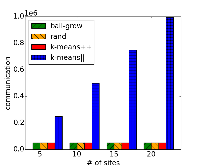
(a)

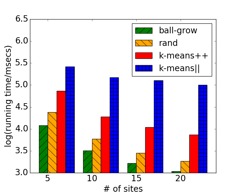
(b)

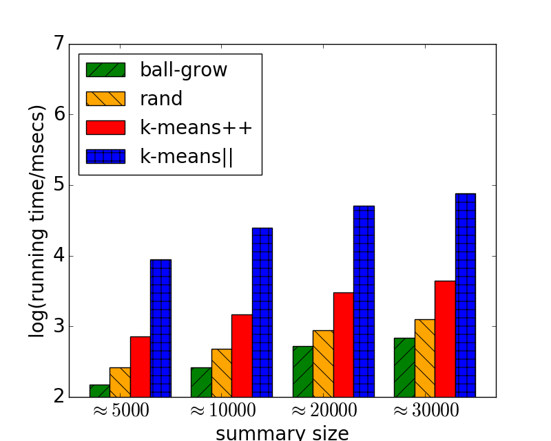
(c)

Figure 1: experiments on kddSp dataset

We next compare the communication cost of different algorithms. Figure 1a presents the experimental results. The communication cost is measured by the number of points exchanged between the coordinator and all sites. In this set of experiments we only change the number of partitions (i.e., # of sites $s$). The summaries returned by all algorithms have almost the same size.

We observe that the communication costs of ball-grow, $k$-means++ and rand are almost independent of the number of sites. Indeed, ball-grow, $k$-means++ and rand all run in one round and their communication cost is simply the size of the union of the $s$ summaries. $k$-means‖ incurs significantly more communication, and it grows almost linearly to the number of sites. This is because $k$-means‖ grows its summary in multiple rounds; in each round, the coordinator needs to collect messages from all sites and broadcasts the union of those messages. When there are $20$ sites, $k$-means‖ incurs $20$ times more communication cost than its competitors.

5.2.3 Running Time

We finally compare the running time of different algorithms. All experiments in this part are conducted on kddSp dataset since $k$-means‖ does not scale to kddFull; similar results can also be observed on other datasets. The running time we show is only the time used to construct the input (i.e., the union of the $s$ summaries) for the second level clustering, and we do not include the running time of the second level clustering since it is always the same for all tested algorithms (i.e., the $k$-means--).

Figure 1b shows the running time when we change the number of sites while fix the size of the summary produced by each site. We observe that $k$-means‖ uses significantly more time than ball-grow, $k$-means++ and rand. This is predictable because $k$-means‖ runs in multiple rounds and communicates more than its competitors. ball-grow uses significantly less time than others, typically $1/25$ of $k$-means‖, $1/7$ of $k$-means++ and $1/2$ of rand. The reason that ball-grow is even faster than rand is that ball-grow only needs to compute weights for about half of the points in the constructed summary. As can be predicted, when we increase the number of sites, the total running time of each algorithm decreases.

We also investigate how the size of the summary will affect the running time. Note that for ball-grow the summary size is controlled by the parameter $t$. We fix $k=3$ and vary $t$, resulting different summary sizes for ball-grow. For other algorithms, we tune the parameters so that they output summaries of similar sizes as ball-grow outputs. Figure 1c shows that when the size of summary increases, the running time increases almost linearly for all algorithms.

5.2.4 Stability of The Experimental Results

Our experiments involve some randomness and we have already averaged the experimental results for multiple runs to reduce the variance. To show that the experimental results are reasonably stable, we add Table 6 to present the standard deviations of the results. For each metric of a given algorithm, we gather $5$ data points, each of which is the averaged result of 10 runs. We then calculate the mean/stddev of the $5$ data points.

algo	$\ell_{1}$-loss	$\ell_{2}$-loss	preRec	prec	recall
ball-grow	$8.16\mathbf{E}5\pm 1.1\mathbf{E}4$	$3.46\mathbf{E}6\pm 4.1\mathbf{E}5$	$0.61\pm 0.002$	$0.55\pm 0.007$	$0.52\pm 0.004$
$k$-means++	$8.83\mathbf{E}5\pm 6.9\mathbf{E}4$	$5.11\mathbf{E}6\pm 2.8\mathbf{E}5$	$0.37\pm 0.004$	$0.36\pm 0.004$	$0.18\pm 0.002$
$k$-means‖	$8.41\mathbf{E}5\pm 5.0\mathbf{E}4$	$4.19\mathbf{E}6\pm 1.4\mathbf{E}5$	$0.29\pm 0.004$	$0.36\pm 0.005$	$0.16\pm 0.004$
rand	$9.20\mathbf{E}5\pm 5.9\mathbf{E}4$	$1.08\mathbf{E}7\pm 2.0\mathbf{E}5$	$0.07\pm 0.001$	$0.49\pm 0.009$	$0.04\pm 0.005$

Table 6: Clustering quality on kddSp  $k=3$, $t=8752$. Each entry is in the format of mean$\pm$stddev.

It can be seen from Table 6 that the results of our experiments are very stable in almost all metrics. $\ell_{1}$-loss is the only metric where our algorithm has some overlap with other baseline algorithms, but it is still safe to conclude that our algorithm outperforms all the baselines in almost all metrics. The similar stability is observed on other datasets.

5.2.5 Summary

We observe that ball-grow gives the best performance in almost all metrics for measuring summary quality. $k$-means‖ slightly outperforms $k$-means++. rand fails completely in the task of outliers detection. For communication, ball-grow, $k$-means++ and rand incur similar costs and are independent of the number of sites. $k$-means‖ communicates significantly more than others. For running time, ball-grow runs much faster than others, while $k$-means‖ cannot scale to large-scale datasets.

Acknowledgments

Jiecao Chen, Erfan Sadeqi Azer and Qin Zhang are supported in part by NSF CCF-1525024 and IIS-1633215.

References

- Arthur and Vassilvitskii (2007) Arthur, D. and Vassilvitskii, S. (2007). k-means++: the advantages of careful seeding. In SODA, pages 1027–1035.
- Bahmani et al. (2012) Bahmani, B., Moseley, B., Vattani, A., Kumar, R., and Vassilvitskii, S. (2012). Scalable k-means++. PVLDB, 5(7), 622–633.
- Balcan et al. (2013) Balcan, M., Ehrlich, S., and Liang, Y. (2013). Distributed k-means and k-median clustering on general communication topologies. In NIPS, pages 1995–2003.
- Baldi et al. (2014) Baldi, P., Sadowski, P., and Whiteson, D. (2014). Searching for exotic particles in high-energy physics with deep learning. Nature communications, 5.
- Charikar et al. (2001) Charikar, M., Khuller, S., Mount, D. M., and Narasimhan, G. (2001). Algorithms for facility location problems with outliers. In SODA, pages 642–651.
- Chawla and Gionis (2013) Chawla, S. and Gionis, A. (2013). k-means-: A unified approach to clustering and outlier detection. In SDM, pages 189–197.
- Chen et al. (2016) Chen, J., Sun, H., Woodruff, D. P., and Zhang, Q. (2016). Communication-optimal distributed clustering. In NIPS, pages 3720–3728.
- Chen (2009) Chen, K. (2009). On coresets for k-median and k-means clustering in metric and euclidean spaces and their applications. SIAM J. Comput., 39(3), 923–947.
- Cohen et al. (2015) Cohen, M. B., Elder, S., Musco, C., Musco, C., and Persu, M. (2015). Dimensionality reduction for -means clustering and low rank approximation. In STOC, pages 163–172.
- Diakonikolas et al. (2017) Diakonikolas, I., Grigorescu, E., Li, J., Natarajan, A., Onak, K., and Schmidt, L. (2017). Communication-efficient distributed learning of discrete distributions. In NIPS, pages 6394–6404.
- Ene et al. (2011) Ene, A., Im, S., and Moseley, B. (2011). Fast clustering using mapreduce. In SIGKDD, pages 681–689.
- Feldman and Schulman (2012) Feldman, D. and Schulman, L. J. (2012). Data reduction for weighted and outlier-resistant clustering. In SODA, pages 1343–1354.
- Guha et al. (2003) Guha, S., Meyerson, A., Mishra, N., Motwani, R., and O’Callaghan, L. (2003). Clustering data streams: Theory and practice. IEEE Trans. Knowl. Data Eng., 15(3), 515–528.
- Guha et al. (2017) Guha, S., Li, Y., and Zhang, Q. (2017). Distributed partial clustering. In SPAA, pages 143–152.
- Gupta et al. (2017) Gupta, S., Kumar, R., Lu, K., Moseley, B., and Vassilvitskii, S. (2017). Local search methods for k-means with outliers. PVLDB, 10(7), 757–768.
- Liang et al. (2014) Liang, Y., Balcan, M., Kanchanapally, V., and Woodruff, D. P. (2014). Improved distributed principal component analysis. In NIPS, pages 3113–3121.
- Lloyd (1982) Lloyd, S. P. (1982). Least squares quantization in PCM. IEEE Trans. Information Theory, 28(2), 129–136.
- Mettu and Plaxton (2002) Mettu, R. R. and Plaxton, C. G. (2002). Optimal time bounds for approximate clustering. In UAI, pages 344–351.
- Sanderson (2010) Sanderson, C. (2010). Armadillo: An open source c++ linear algebra library for fast prototyping and computationally intensive experiments.