Current-Induced Heat Transfer in Double-Layer Graphene

Abstract

Using the fluctuational electrodynamics and nonequilibrium Green’s function methods, we demonstrate the existence of a current-induced heat transfer in double-layer graphene even when the temperatures of the two sheets are the same. The heat flux is quadratically dependent on the current. When temperatures are different, external voltage bias can reverse the direction of heat flow. The drift effect can exist in both macroscopic and nanosized double-layer graphene and extend to any other 2D electron systems. These results pave the way for a different approach to the thermal management through radiation in nonequilibrium systems.

I Introduction

Understanding and controlling the heat flow is a significant endeavor both in nonequilibrium statistical physics and in practical applications. Managing radiative heat transfer (RHT) at small scales is essential for the development of a wide variety of technologies, including phononics Li et al. (2012), near-field thermophotovoltaics Basu et al. (2009) and thermal photonic analog of electronic devices Ben-Abdallah and Biehs (2014). In the last decades, near-field radiative heat transfer (NFRHT) Song et al. (2015), where the separation distance is smaller than Wien’s wavelength, has been proposed to enhance the RHT through surface-plasmon polariton Joulain et al. (2005), surface-phonon polariton Shen et al. (2009), and so on. The NFRHT between different materials, such as semiconductor or bilayer graphene, can be electronically controlled by the photon chemical potential or gate voltage bias Chen et al. (2015); Ilic et al. (2012); Yu et al. (2017); Peng et al. (2015). Moreover, the novel electrically manipulated properties of 2D materials can give an additional knob to tune the RHT in nonequilibrium conditions.

Here we explore the RHT between two graphene layers (double-layer graphene) across a separation gap by drifting one of the layers with a constant drift velocity or voltage bias, through modeling by the fluctuational electrodynamics (FE) and nonequilibrium Green’s function (NEGF), respectively. We demonstrate the existence of drift-induced RHT in double-layer graphene, with intensity depending quadratically on the drift velocities or voltage bias. The RHT produced by the temperature imbalance can even be suppressed by drift-induced RHT, and the heat flux can be switched off by the voltage bias. We interpret that this drift effect is related to the negative Landau damping in grapheneMorgado and Silveirinha (2017). The physics is generic and it appears in between bulk graphene sheets or nanosized flecks.

We consider a two-layer graphene system, where the bottom and top layer are labeled by 1 and 2 respectively, separated by a vacuum gap of distance $d$, and emitting thermal radiation at temperatures $T_{1(2)}$. Figure 1 schematically illustrates the configuration under our investigation. There is an electric current induced by a static voltage applied across the bottom layer of graphene. Due to the high mobility of graphene, the drift velocity of electrons in graphene can be on the order of the Fermi velocity of graphene, i.e., $10^{6}\,\mathrm{m/s}$.

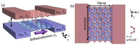
Figure 1: Scheme of a double-layer system under investigation: two graphene layers separated with a vacuum gap $d$. The chemical potential difference ($\mu_{1R}-\mu_{1L}$) induces electron drift in the bottom graphene layer, (a) perspective view, (b) top view.

II Fluctuational electrodynamics description

We generalize the usual formula for heat transfer, for which local equilibrium in each layer is assumed. Due to the current in the bottom layer, the system is intrinsically not in local thermal equilibrium. This nonequilibrium situation is taken care by a simple hypothesis of an energy shift in the distribution functions. When the bottom layer 1 is driven by a drift velocity $v_{1}$ in $x$ direction and there is no drift in the top layer, the photon distribution is Doppler shifted on the bottom layer. Thus, the Bose function becomes:

$$N_{1}(\omega,k_{x})=\frac{1}{e^{\frac{\hbar(\omega-k_{x}v_{1})}{k_{b}T_{1}}}-1},$$ (1)

where $k_{x}$ is the wave number along $x$ direction. $k_{b}$ is the Boltzmann constant. Under the relaxation time approximation, the drift-induced distribution is similar to the distribution with chemical potential of photon in semiconductors. The heat transfer rate per unit area between the layers of graphene is then given under FE as Rytov (1959); Volokitin and Persson (2007):

$$H=\int_{0}^{\infty}\frac{d\omega}{2\pi}\int\frac{d^{2}{\bf k}_{\perp}}{(2\pi)^{2}}\Theta_{12}(\omega,k_{x})\mathrm{T}_{12}(\omega,{\bf k}_{\perp}),$$ (2)

where $\omega$ is the frequency of electromagnetic wave. ${\bf k}_{\perp}=(k_{x},k_{y})$ is the wavevector in the graphene plane. $\Theta_{12}(\omega,k_{x})\equiv\hbar\omega\bigl{[}N_{1}(\omega,k_{x})-N_{2}(\omega)\bigr{]}$. $N_{2}(\omega)$ is the usual Bose function at temperature $T_{2}$. $\mathrm{T}_{12}(\omega,{\bf k}_{\perp})$ is the transmission coefficient.

For an infinitely large suspended double-layer graphene with nanoscale separation, the $p$-polarized wave is the dominant channel for RHT Ilic et al. (2012). Based on FE, the transmission for evanescent $p$-polarized modes between a pair of two-dimensional materials in a parallel plate geometry can be written as (in the non-retardation limit, the speed of light $c\to\infty$) Polder and Van Hove (1971); Pendry (1999); Volokitin and Persson (2007):

$$\mathrm{T}_{12}(\omega,{\bf k}_{\perp})=\frac{4\,\mathrm{Im}(r_{1})\,\mathrm{Im}(r_{2})}{|1-r_{1}r_{2}e^{-2\gamma d}|^{2}}e^{-2\gamma d},$$ (3)

where $r_{1}$ and $r_{2}$ are the reflection coefficients at the bottom and top interface of the vacuum gap. $d$ is the distance of the vacuum gap. $\gamma=\sqrt{k_{x}^{2}+k_{y}^{2}}$. The drifted reflection coefficient is computed according to $r_{1}=v_{{\bf k}_{\perp}}\Pi(\omega,{\bf k}_{\perp},v_{1})/\bigl{[}1-v_{{\bf k}_{\perp}}\Pi(\omega,{\bf k}_{\perp},v_{1})\bigr{]}$. The bare Coulomb interaction in wavevector space in two dimensions is $v_{{\bf k}_{\perp}}=1/(2\epsilon_{0}\gamma)$. $r_{2}$ is computed at no drift ($v_{1}=0$). We calculate the drifted polarization function following the approximation of Svintsov et al.Svintsov and Ryzhii (2018):

$$\Pi_{{\bf k}_{\perp}}(\omega,v_{1}) = \frac{e^{2}\mu(T_{i})}{(\pi\hbar v_{F})^{2}}\int_{0}^{2\pi}\!d\theta\,\frac{1}{(1-\beta\cos\theta)^{2}}\times\qquad$$ (4)

$$\frac{k_{x}(\cos\theta-\beta)+k_{y}\sin\theta}{(\hbar\omega+i\eta)/(\hbar v_{F})-k_{x}\cos\theta-k_{y}\sin\theta},\quad$$

where we define $\beta=v_{1}/v_{F}$, the Fermi velocity is $v_{F}=\frac{3}{2}at/\hbar$ with carbon bond length $a=1.42\,$Å and hopping parameter $t=2.8\,$eV, and $\eta$ is a small electron damping parameter, which gives graphene a finite DC conductivity. Finally, $\mu(T)=2k_{b}T\ln[2\cosh\frac{\mu}{2k_{b}T}]$. The long-wave approximation (${\bf k}_{\perp}$ small) is valid as the contribution of the transmission is concentrated around $\gamma\sim O(1/d)$. The appendices further discuss details of the approximations and calculations.

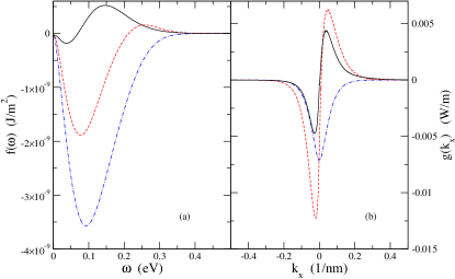
Figure 2: (a) Integrated spectral transfer function $f(\omega)$ as a function of frequency and (b) $g(k_{x})$ as a function of wave vector, with different drift velocities: no drift (blue dash-dot line), total heat current density $H=-0.84\,$MW/m², $v_{1}=5.0\times 10^{5}\ \mathrm{m/s}$ (red dash line), $-0.30\,$MW/m², and $v_{1}=9.0\times 10^{5}\ \mathrm{m/s}$ (black solid line), $+0.09\,$MW/m². The temperatures are $T_{1}=300\,$K and $T_{2}=320\,$K. The chemical potential of graphene $\mu$ is set as 0.1 eV. Gap distance $d$ is set as 10 nm. The damping parameter is $\eta=9\,$meV.

To understand the drift effects quantitatively, we define two integrated spectral transfer functions as follows:

$$f(\omega)=\int\frac{d^{2}{\bf k}_{\perp}}{(2\pi)^{3}}\Theta_{12}(\omega,k_{x})\mathrm{T}_{12}(\omega,{\bf k}_{\perp}),$$ (5)

$$g(k_{x})=\int_{0}^{\infty}\frac{d\omega}{2\pi}\int\frac{dk_{y}}{(2\pi)^{2}}\Theta_{12}(\omega,k_{x})\mathrm{T}_{12}(\omega,{\bf k}_{\perp}).$$ (6)

Figure 2(a) shows the spectral transfer function $f(\omega)$ as a function of frequency with different drift velocities. In the undriven case (blue dash-dot), $f(\omega)$ is strictly negative and the heat current flows from top layer to bottom layer due to the temperature difference ($T_{1}=300$ K and $T_{2}=320$ K). It is the usual RHT between two graphene layers and the RHT can be tuned by doping or top gating (varying $\mu$). However, when the electrons in the bottom layer are drifted with a velocity $v_{1}=5.0\times 10^{5}\mathrm{m/s}$ (red dash line) in Fig. 2(a), corresponding to an electric line current density $j_{1}=(-e)n_{1}v_{1}=486$ A/m, there is a small positive peak in $f(\omega)$. That means that part of the high-frequency modes can spontaneously emit external thermal radiation from bottom layer to top layer due to the drift velocity. Remarkably, with a higher drift velocity (black solid line), the height of the peak in the high-frequency region grows higher, and there is more heat transferred from bottom layer to the top layer. Qualitatively, the heat flux generated by a temperature difference can be suppressed or even reversed by the high drift velocity.

The above mentioned drift-induced effects in suspended layers can be further understood in Fig. 2(b): the distribution over the wavevector in the $\hat{x}$ (the driven) direction. In no drift case, $g(k_{x})$ is negative and has the space inversion symmetry in $x$ direction. However, when we drift the electrons in $x$ direction, the $k_{x}$ symmetry is broken and the drift induced mode appears. In the $k_{x}<\omega/{v_{1}}$ and $\omega>0$ region, it is negative and the system locates at the normal Landau damping region. However, when $k_{x}>\omega/{v_{1}}$ and $\omega>0$, the drift induced modes carry positive value due to negative Landau damping. The total heat current is from contributions of all those modes. In low frequency region ($\omega<0.1$ eV), the heat flux is dominated by the normal Landau damping modes. In high frequency region ($\omega>0.1$ eV), the negative Landau damping modes can be the dominant modes for heat transfer. Due to the unsymmetric nature with an $x$-direction drift current, heat can be transferred from low temperature layer to high temperature layer through the negative Landau damping modes.

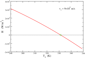
Figure 3: Heat current density as a function of $T_{2}$ (temperature of the top layer) with drift velocity $v_{1}=9.0\times 10^{5}\ \mathrm{m/s}$ (red solid line). Dotted line is the reference line for zero current density. The green circle indicates the point for “off temperature”. The chemical potential of graphene $\mu$ is set as 0.1 eV. Temperature of bottom layer of graphene $T_{1}$ is set as 300 K. Vacuum gap distance $d$ is set as 10 nm.

With the help of drift effects, we have demonstrated that the RHT in double-layer graphene can be tuned by the drift velocity, even shutting off or changing sign. To gain a detailed picture of the drift effects, we calculate the heat current density as a function of ${T_{2}}$ with fixed drift velocity $v_{1}=9.0\times 10^{5}$ m/s. As seen in Fig. 3, the heat current density is almost linearly decreasing as the temperature $T_{2}$ increases. When $T_{2}$ equals 331 K, there is no heat current between the layers and the “off temperature” for RHT is reached.

III Nonequilibrium Green’s function calculation

The above calculation is based on FE for the infinite suspended double-layer graphene. To extend drift induced effect in the nanoscale system, we consider a small graphene nano-ribbon of 72 atoms in each layer (see Fig. 1), connected to two baths, in each layer. The chemical potential difference ($\mu_{1R}-\mu_{1L}$) between bath 1L and bath 1R produces the drift electrons in layer 1. In such a nanoscale system, the Coulomb interaction (virtual photon or scalar photon) will be the dominant mechanism for RHT.

The calculation is based on a tight-binding model with a nearest neighbor hopping parameter $t=2.8$ eV and Coulomb interactions between the electrons Zhang et al. (2018); Wang et al. (2018); Peng et al. (2017). The energy transfer out of layer 1 to layer 2 of a nanoscale double-layer graphene due to the Coulomb interaction can be calculated through the Meir-Wingreen formula Lü et al. (2016, 2015); Meir and Wingreen (1992) under a lowest order expansion of the Coulomb interaction (see Appendix D for a derivation):

$$H=-\frac{1}{A}\int_{0}^{+\infty}\frac{d\omega}{2\pi}\hbar\omega{\rm Tr}(D^{>}\Pi^{<}_{1}-D^{<}\Pi^{>}_{1}).$$ (7)

Here $D^{>,<}$ is the greater/lesser Green’s function for the scalar photon, which is calculated from the Keldysh equation, $D^{<,>}=D^{r}\Pi^{<,>}D^{a}$, and retarded Green’s function is obtained by solving the Dyson equation, $D^{r}=v+v\Pi^{r}D^{r}$ ($v$ is the bare Coulomb potential with matrix element $1/(4\pi\epsilon_{0}r_{ij})$ between the tight-binding sites $i$ and $j$ of a distance $r_{ij}$). $\Pi^{<,>}=\Pi^{<,>}_{1}+\Pi^{<,>}_{2}$ is block-diagonal and is obtained with the random phase approximation (RPA). $A$ is the area of the graphene. Further computational details will be presented in Appendix E.

Comparing with the calculation based on FE, the NEGF method provides a rigorous way to extend the drift effects into nanoscale ballistic systems without any phenomenological assumptions. Due to the smallness of the sample, the transport is ballistic with the electric current at the bottom driven layer given by $I_{1}=(4e/h)(\mu_{1R}-\mu_{1L})$, independent of the sample width or length. We do not observe Coulomb drag effect Narozhny and Levchenko (2016), as the electric current in the top unbiased layer is very close to 0, while the thermal current going into it is quite large, see Fig. 4(b). From the view of energy transport, the energy can be transferred from an electrically driven layer to the closely spaced but electrically isolated layer: the drift electrons are dragged by the Coulomb interaction between two layers, and the energy can be transferred at the cost of the kinetic energy of drift electrons.

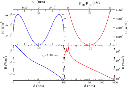
Figure 4: (a) FE calculation of drift-induced heat current density as a function of drift velocity. Vacuum gap distance $d$ is set as 10 nm. The chemical potential of graphene $\mu$ is set as 0.1 eV. (b) NEGF calculation of drift-induced heat current density as a function of chemical potential difference $\mu_{1R}-\mu_{1L}$ symmetrically biased and $\mu_{2L}=\mu_{2R}=0.1\,\mathrm{eV}$. Vacuum gap distance $d$ is set as 1 nm. (c) FE drift-induced heat current density as a function of gap distance with drift velocity $v_{1}=7.0\times 10^{5}\,$m/s. (d) NEGF drift-induced heat current density as a function of gap distance with $\mu_{1R}=0.15$ eV, $\mu_{1L}=0.05\,$eV and $\mu_{2L}=\mu_{2R}=0.1\,$eV. There is no temperature difference between the double-layer graphene, $T_{1}=T_{2}=300\,$K.

Huge heat transfer appears even for $T_{1}=T_{2}$, which is clearly due to strong Coulomb interactions at short distances. A comparison of FE and NEGF results is presented in Fig. 4. Using FE method, Fig. 4(a) indicates the drift-induced heat current density as a function of drift velocity with both layers at the same temperature. A parabolic dependence between drift-induced heat current and drift velocity is found numerically for small $v_{1}$. For large drift exceeding $|v_{1}|>7.0\times 10^{5}\,$m/s, we see non-monotonic behavior. From the NEGF point of view, the chemical potential difference between left and right bath can produce an electric current and it is similar to the drift electron one in FE calculation. In Fig. 4(b), we found that the heat current density also quadratically depends on the chemical potential difference $\mu_{1R}-\mu_{1L}$. In our symmetric setup, we do not expect that the heat transfer will be different if we reverse the direction of the drift velocity or voltage bias, so it must depend on them quadratically. It is tempting to assume that the heat transfer is given by Joule heating caused by Coulomb drag. Unfortunately, this is not quite true (see Appendix C).

Further numerical evidence is shown in Fig. 4(c) and (d): the distance dependence of drift-induced heat current. Fig. 4(c) depicts the drift-induced heat current density as a function of distance under FE calculation with fixed drift velocity. We observe that the drift induced heat current decays initially as $d^{-4}$ when the gap distance is smaller than 10 nm and decreases as $d^{-2}$ when $d>10$ nm. A similar distance dependence is also observed in Fig. 4(d) for the nanosize sample with a larger range of $d^{-2}$ behavior.

In summary, we proposed methods to describe heat transport without the assumption of local equilibrium. With FE method, the Bose function and Fermi function need to be shifted due to the drift velocity. For NEGF, we give a Meir-Wingreen formula with the input from a RPA calculation for $\Pi^{r}$ where the electron Green’s function is current-carrying and not in thermal equilibrium. We have demonstrated a drift induced radiative heat transfer in double-layer graphene. Such effects can be extended to any other 2D electron systems with large drift velocity or current. The drift induced heat current can even shut off the heat current produced by a temperature difference. It enables possibilities to exploit RHT through electronic control. Further, the proposed drift effects can exist in both large and microscopical systems. With wide-band tunability and nano-scale characteristic dimensions, the proposed drift effects appear very charming for the application in radiative thermal management.

Appendix A Doppler shift

In the appendices, we clarify some points made in the main texts and give some further details.

We first note that the function $\Pi^{r}_{\bf k}(\omega)$ is a description of the bosonic charge density plasmon. In particular, we consider a plasmon planewave $e^{i({\bf k}\cdot{\bf r}-\omega t)}$ with frequency $\omega$ and wavevector ${\bf k}$. Let ${\bf v}_{1}$ describe the drift velocity of the electrons. If the wave ${\bf k}$ of the plasmon and the electron drift velocity ${\bf v}_{1}$ are in the same direction, electrons will “see” less vibrations, thus $\omega$ decreases. So the Doppler shift is, $\omega\rightarrow\omega+\delta\omega=\omega-{\bf k}\cdot{\bf v}_{1}=\omega-k_{x}v_{1}$.

Appendix B Doppler shift or not for scalar photon self-energy

The scalar photon self energies or polarization functions under the random phase approximation are, in time domain and real space,

$$\Pi_{jk}^{>}(t) = (-i\hbar)e^{2}G_{jk}^{>}(t)G_{kj}^{<}(-t),$$ (8)

$$\Pi_{jk}^{<}(t) = (-i\hbar)e^{2}G_{jk}^{<}(t)G_{kj}^{>}(-t),$$ (9)

$$\Pi_{jk}^{r}(t) = \theta(t)\bigl{(}\Pi_{jk}^{>}(t)-\Pi_{jk}^{<}(t)\bigr{)}.$$ (10)

We obtain the frequency and wavevector domain quantities if we Fourier transform the time and space. For simplicity of notation, we consider spinless electrons with a single band, $\epsilon_{\bf k}$. Since the system is not in thermal equilibrium, we cannot evoke the usual fluctuation-dissipation theorem, but something very close to it. We use the Kadanoff-Baym ansatz Kadanoff and Baym (1962), i.e.,

$$G^{<}=-f(G^{r}-G^{a}),\quad G^{>}=(1-f)(G^{r}-G^{a}),$$ (11)

where $f$ is given by the solution of Boltzmann equation. The spectrum function, $A=i(G^{r}-G^{a})$, is assumed to be evaluated in thermal equilibrium. In wavevector and angular frequency domain, we can write Mahan (2000); Duppen et al. (2016)

$$\Pi^{r}_{\bf k}(\omega)=-e^{2}\int\frac{d^{2}\bf p}{(2\pi)^{2}}\frac{f_{\bf p}-f_{{\bf p}-{\bf k}}}{\hbar\omega+i\eta-\epsilon_{\bf p}+\epsilon_{{\bf p}-{\bf k}}}.$$ (12)

Here the integration is over the first Brillouin zone, and $\eta$ is a small damping parameter inversely proportional to the relaxation time.

As the relaxation mechanism for the electrons can be very complicated due to different scattering possibilities – impurity scatterings, electron-electron and electron-phonon scatterings – we do not attempt to solve the Boltzmann equation, and just use a single-mode relaxation time approximation Ziman (1960). In such a framework, we can write

$$f=f^{0}-\frac{df^{0}}{d\epsilon}\Phi\approx f^{0}(\epsilon-\Phi),$$ (13)

here $\Phi\equiv\Phi_{\bf k}$ is mode ${\bf k}$ dependent, and $f^{0}=1/\bigl{[}\exp((\epsilon-\mu)/(k_{b}T))+1\bigr{]}$ is the equilibrium Fermi distribution at temperature $T$ and chemical potential $\mu$.

The effect of the current drift is to introduce anisotropy to the problem, thus we expect $\Phi$ should be angle and magnitude dependent, $\Phi_{\bf k}=\Phi(\theta,k)$, here $\theta$ is the angle between ${\bf k}$ and the drift velocity ${\bf v}_{1}$ and $k=|{\bf k}|$ is the magnitude of the wavevector. We make a Legendre polynomial expansion of the angular dependence and keep only the lowest non-trivial term, i.e., we write, $\Phi\propto\cos(\theta)$. It is convenient to assume

$$\Phi_{\bf k}=\hbar k_{x}v_{1}=\hbar v_{1}k\cos\theta.$$ (14)

If $\Phi$ does take this linear dependence on $k_{x}$, the nonequilibrium distribution might be transformed back to the equilibrium one of $f^{0}$ by a change of reference frame. That is,

$$\Pi^{>,<,r}_{{\bf k},\rm noneq}(\omega)\approx\Pi^{>,<,r}_{{\bf k},\rm eq}(\omega-k_{x}v_{1}).$$ (15)

In steady state, the fluctuation-dissipation like relation for photon self-energy can be obtained from Eq. (15) even if there is drifted electron current:

$$\Pi^{<}_{{\bf k},\rm noneq}(\omega)=2iN_{{\bf k},\rm noneq}(\omega)\mathrm{Im}\Pi^{r}_{{\bf k},\rm noneq}(\omega),$$ (16)

$$N_{{\bf k},\rm noneq}(\omega)\approx N(\omega-k_{x}v_{1}),$$ (17)

where $N(\omega)=1/(e^{\hbar\omega/(k_{b}T)}-1)$ is the Bose distribution.

The reflection coefficient needed for the heat transfer calculation is then obtained from the relation $r=v\Pi^{r}/(1-v\Pi^{r})$ with bare Coulomb potential in two dimensions $v=1/(2\epsilon_{0}k)$. The optical conductivity is related to the retarded self energy by $\sigma=i\frac{\omega}{k^{2}}\Pi^{r}_{\bf k}(\omega)$.

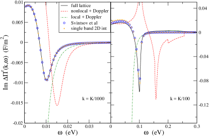
Figure 5: Imaginary part of $\Pi^{r}({\bf k},\omega,v_{1})-\Pi^{r}({\bf k},\omega,0)$, with ${\bf k}=(k_{x},0)$, $v_{1}=5\times 10^{5}$ m/s, at chemical potential $\mu=0.1\,$eV. Left graph has $k_{x}=K/1000$ and right 10 time larger, $K=4\pi/(3\sqrt{3}a)$ is the magnitude of the K-point vector from the $\Gamma$ point, $a=1.42\,$Å is carbon bond length. Temperature is set at 100 K. A damping parameter in $\hbar\omega\to\hbar\omega+i\eta$ is set to $\eta=3.3\,$meV. The legends apply to both graphs, full black solid line: tight-binding lattice model with nearest neighbor hopping parameter $t=2.8\,$eV, red dash line: Doppler shifted Wunsch et al. expression, green dot-dash line: Doppler shifted Falkovsky’s expression, blue circles: Svintsov et al expression, orange pluses: numerical integration of Eq. (12).

For a quadratic dispersion relation, $\epsilon_{\bf k}=\hbar^{2}k^{2}/(2m)$, the claim, Eq. (15), is easily verified using the explicit expression for $\Pi^{r}$, Eq. (12), by a change of integration variable with a constant shift, ${\bf p}\to{\bf p}+m{\bf v}_{1}/\hbar$. For graphene with Dirac cone, $\epsilon_{\bf k}=v_{F}\,\hbar k$, this is no longer true. A variable transform cannot eliminate both $\Phi_{\bf p}$ and $\Phi_{{\bf p}-{\bf q}}$ simultaneously. As a result, Doppler shift of the equilibrium result and nonequilibrium distribution in the Fermi function becomes inequivalentSvintsov and Ryzhii (2018). The energy shift needs to be momentum dependent. The linear dependence on $k_{x}$ times a constant requires a specific assumption on the energy dependence of the relaxation times. According to the usual relaxation time approximation, $\Phi$ is given by (near $K$ or $K^{\prime}$ points)

$$\Phi=-eE\tau_{k}\frac{\partial\epsilon_{\bf k}}{\partial(\hbar k_{x})},$$ (18)

where electron carries charge $-e$, $E$ is the applied electric field in $x$ direction, $\tau_{k}$ is the relaxation time assumed to only depend on the magnitude of ${\bf k}$, and the last factor is the group velocity. For a metal with the usual quadratic dispersion, Eq. (14) is true if we use constant relaxation time, which turns out to be very good approximation for metal. For graphene, the group velocity in $x$-direction is $v_{F}\cos(\theta)$ with the Fermi velocity a constant, thus we must demand a relaxation time proportional to $k$, which turns out in agreement with experiments Neto et al. (2009).

For a full lattice model numerical calculation such that $\Phi_{\bf k}$ respects the lattice symmetry, we take the drift term to be $\Phi_{\bf k}=v_{1}{\rm Re}\left[z^{*}\frac{\partial z}{\partial k_{x}}\right]/(\hbar v_{F}^{2})$, where $v_{F}=3at/(2\hbar)$ is the graphene Fermi velocity, and $z=-t(e^{-ik_{x}a}+e^{i(k_{x}a/2+k_{y}a\sqrt{3}/2)}+e^{i(k_{x}a/2-k_{y}a\sqrt{3}/2)})$. In Fig. 5, we compare Doppler shifted Wunsch et al. expression Wunsch et al. (2006) (or that of Hwang and Sarma Hwang and Sarma (2007)) which is a nonlocal result at zero temperature or that of Falkovsky’s small $q$ (local) resultFalkovsky (2008) at $T=100\,$K. As we can see they differ a lot and do not agree with the correct way of evaluating the drifted polarization function. On this scale of vertical axis, they also tend to diverge to plus or minus infinity. However, Svintsov et al. expression Svintsov and Ryzhii (2018) (with a correction of a sign error in the denominator),

$$\Pi^{r}_{(k_{x},k_{y}\!=\!0)}(\omega,v_{1}) = -\frac{2}{\pi}\frac{e^{2}\mu}{(\hbar v_{F})^{2}}\frac{1}{(1-s\beta)^{2}}\Bigg{(}\qquad\qquad\qquad$$ (20)

$$\qquad\sqrt{1-\beta^{2}}-\frac{s-\beta}{\sqrt{s^{2}-1}}\Bigg{)},$$

$$\beta = {\rm sgn}(k_{x})\frac{v_{1}}{v_{F}},\quad s=\frac{\hbar\omega+i\eta}{\hbar|k_{x}|v_{F}},$$ (21)

agrees very well with a full lattice model calculation Jiang and Wang (2017). When the chemical potential is much larger than $k_{b}T$ and at $\omega>v_{F}k\to 0$, we have an excellent approximation for the equilibrium polarization

$$\Pi^{r}_{\bf k}(\omega)\approx\frac{e^{2}\mu}{\pi}\frac{k^{2}}{(\hbar\omega+i\eta)^{2}}.$$ (22)

Doppler shift of this expression in the small $v_{1}$ limit gives $\Delta\Pi^{r}=\Pi^{r}(v_{1})-\Pi^{r}(0)\approx 2D$, while Svintsov et al. expression in this limit is $-D$, where $D=(e^{2}\mu/\pi)\hbar v_{1}[k/(\hbar\omega+i\eta)]^{3}$. Both the sign and magnitude are different, contrary to the claim in ref. Morgado and Siveirinha, 2018.

Appendix C Possible connection to Coulomb drag

Since we expect that the drift velocity $v_{1}$ is a small quantity, we can make linear, or rather, quadratic response calculations. Taylor expanding in variable $\delta\omega=-k_{x}v_{1}$ of the distribution $N_{1}$ of Eq. (1) in the main text to second order and the transmission function to first order, and then substituting into Eq. (2), and setting the temperatures $T_{1}=T_{2}=T$, we obtain

$$H = \int_{-\infty}^{+\infty}\!\!\frac{d\omega}{4\pi}\hbar\omega\int\frac{d^{2}{\bf k}}{(2\pi)^{2}}T_{12}({\bf k},\omega)\Big{|}_{v_{1}=0}\frac{1}{2}\frac{\partial^{2}N}{\partial\omega^{2}}\bigl{(}\delta\omega\bigr{)}^{2}$$

$$+ \int_{-\infty}^{+\infty}\!\!\frac{d\omega}{4\pi}\hbar\omega\int\frac{d^{2}{\bf k}}{(2\pi)^{2}}\frac{\partial T_{12}({\bf k},\omega)}{\partial v_{1}}\Big{|}_{v_{1}=0}\frac{\partial N}{\partial\omega}\bigl{(}v_{1}\delta\omega\bigr{)}.$$

The first order term proportional to $\delta\omega$ is 0 because it is an odd function in $k_{x}$. We will write this long expression as $H=a\,v_{1}^{2}=(a_{1}+a_{2})v_{1}^{2}$ where $a_{1}$ is from the $(\delta\omega)^{2}$ term and $a_{2}$ from the cross term. The coefficient $a_{2}$ is complicated, hence we focus only on $a_{1}$. Since the integral over $k_{x}^{2}$ and $k_{y}^{2}$ factor is the same, we symmetrize the formula about $x$ and $y$ and divide by two. With further simplification of the second derivation of the Bose function, we obtain

$$a_{1}=\int_{-\infty}^{+\infty}\frac{d\omega}{4\pi}\int\frac{d^{2}{\bf k}}{(2\pi)^{2}}\frac{T_{12}({\bf k},\omega)\,k^{2}(\beta\hbar)^{2}\hbar\omega}{16\sinh^{2}(\frac{\beta\hbar\omega}{2})\tanh(\frac{\beta\hbar\omega}{2})}.$$ (23)

Here $T_{12}$ is defined in the main text by Eq. (3), evaluated at $v_{1}=0$, $\beta=1/(k_{b}T)$. Finally, we make one approximation, that is to assume $\tanh(x)\approx x$ valid if frequency is small in comparison with temperature. Then, we find

$$a_{1}\approx e^{2}n_{1}^{2}\rho_{D},$$ (24)

if we compare our formula with that of Jauho and SmithJauho and Smith (1993) (Eq. (5) and (27)) and that of Flensberg and HuFlensberg and Hu (1995) (Eq. (2) and (20)). Here $n_{1}$ is the carrier surface density and $\rho_{D}$ is the Coulomb drag coefficient. Because of the existence of the second term, $a_{2}$, we don’t have a simple interpretation of Joule heating due to Coulomb drag. Numerically, for the parameters used for Fig. 4(a) in the main texts, we find $a_{1}=5.5\times 10^{-6}\,$Ws²/m⁴, while $a_{2}=-4.3\times 10^{-6}\,$Ws²/m⁴. There is a cancellation effect, given a smaller overall $a$.

Appendix D Numerical calculation of the NEGF conjunction system

For the 4-terminal junction double-layer system discussed in the main texts, wave-vector is not a good quantum number and we cannot study finite size transport in ${\bf k}$ space. As a result, we do calculation in real space with the electron Green’s functions $G_{jk}^{>,<,r}$ where $j$ and $k$ runs over the sites of top and bottom layers of graphene. The retarded Green’s function is calculated in energy space with $G^{r}(E)=(EI-H_{C}-\Sigma^{r})^{-1}$ where $\Sigma^{r}$ is the sum of total self energies due to the four leads. Actually, both $H_{C}$ and $\Sigma^{r}$ are block diagonal with respect to the layer index since there is no direct electronic coupling. As a result, $G^{>,<,r}$ is also block diagonal. The lead self energies are calculated by standard iterative algorithms of surface Green’s functions.

The polarization functions $\Pi^{>,<,r}$ are calculated according to the time-domain formulas and then Fourier transformed to frequency domain. This appears very fast computationally, but it brings about numerical instability for large systems. $4\times 4$ system with about 200 atoms is probably the largest system we can obtain reliable result from. We have used 23000 fast Fourier transform points with a spacing $\hbar\Delta\omega=22$ meV. The nonequilibrium information is incorporated through the lead temperatures and chemical potentials by the Keldysh equation, $G^{<}=G^{r}\Sigma^{<}G^{a}$, at the very beginning when calculating the polarization function $\Pi^{>,<}$, and not through somewhat ad hoc procedure such as Doppler shifting the Bose function. $D^{r}$ is obtained with the Dyson equation, $D^{r}=v+v\Pi^{r}D^{r}$, and $D^{>,<}$ is obtained by the corresponding Keldysh equation. Since we are in real space, we have used periodic boundary conditions in the $y$ direction perpendicular to the transport direction, and have set the diagonal $v_{ii}=0$. Finally, the heat current is calculated according to the formula given in the main texts, Eq. (7). The electric current can also be calculated, using the lowest order expansion formula for the interacting Green’s function given in the next section, with the Meir-Wingreen formula for electric current.

Appendix E Proof of the scalar photon Meir-Wingreen formula, Eq. (7)

We give a derivation of the Meir-Wingreen formula for scalar photon in terms of the Meir-Wingreen formula for the electrons under the lowest order of expansion approximation Paulsson et al. (2005); Lü et al. (2016). We consider a two-layer setup with four leads, layer 1 with left and right lead, and layer 2 left and right lead. The energy current out the layer $\alpha$ is Meir and Wingreen (1992); Lü et al. (2015)

$$I_{\alpha}=\int_{-\infty}^{+\infty}\frac{dE}{2\pi\hbar}E\,{\rm Tr}\bigl{(}G^{>}\Sigma_{\alpha}^{<}-G^{<}\Sigma_{\alpha}^{>}\bigr{)}.$$ (25)

Here $G^{>}$ and $G^{<}$ are the full interacting greater and lesser Green’s functions of the electrons and $\Sigma_{\alpha}^{>,<}=\Sigma_{\alpha,L}^{>,<}+\Sigma_{\alpha,R}^{>,<}$ are the total lead self energies. They are functions of energy $E$. This formula is exact provided that the electron Green’s function is obtained exactly. However, such a goal for the Coulomb system is not attainable. Thus, we use the lowest order expansion approximation in terms of the Coulomb interaction. Such approximation preserves energy conservation exactly. Since the two layers are not coupled directly, the Green’s functions for the electrons and self energies are block diagonal, and the Meir-Wingreen formula needs only the block $\alpha$. We focus on layer 1, and Green’s function $G_{1}^{>}$, can be expressed by the Keldysh equation as

$$G_{1}^{>}=\bigl{[}G^{r}(\Sigma_{1}^{>}+\Sigma_{2}^{>}+\Sigma_{n}^{>})G^{a}\bigr{]}_{11}.$$ (26)

Here $\Sigma_{1,2}^{>}$ are the lead self energies, and $\Sigma_{n}^{>}$ is the Fock term of Coulomb interaction, all of them block diagonal. For the 11-subblock, $\Sigma_{2}$ is 0. Putting this result into the Meir-Wingreen formula, noting that ${\rm Tr}(G_{1}^{>}\Sigma_{1}^{<}-G_{1}^{<}\Sigma_{1}^{>})=0$ as a consequence of charge and energy conservation when Coulomb interaction is turned off, we obtain

$$I_{1}=\int_{-\infty}^{+\infty}\frac{dE}{2\pi\hbar}E\,{\rm Tr}\bigl{[}G^{r}_{1}\Sigma_{n}^{>}G_{1}^{a}\Sigma_{1}^{<}-({\rm swap\ }{}^{>}\leftrightarrow{}^{<})\big{]}.$$ (27)

From now on we will drop the subscript 1 for notational simplicity.

A key approximation we use is the lowest order expansion,

$$G^{>}\approx G_{0}^{>}+G_{0}^{r}\Sigma_{n}^{r}G_{0}^{>}+G_{0}^{r}\Sigma_{n}^{>}G_{0}^{a}+G_{0}^{>}\Sigma_{n}^{a}G_{0}^{a}.$$ (28)

We obtain such terms if we expand the contour ordered Dyson equation, $G=G_{0}+G_{0}\Sigma_{n}G\approx G_{0}+G_{0}\Sigma_{n}G_{0}+\cdots$, and then take the greater component using the Langreth rule Haug and Jauho (1996). We also drop the subscript 0 from now on.

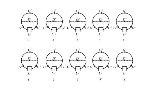
Figure 6: Diagrams for heat current in lowest order expansion.

It is useful for symmetry reasons we express the current by vacuum diagrams in time domain. We use the inverse Fourier transform to change the integral in energy to time, and also the Fock diagram result, $\Sigma_{n}^{>}(t,t^{\prime})=i\hbar\sum_{l,l^{\prime}}M^{l}G^{>}(t,t^{\prime})M^{l^{\prime}}D_{l,l^{\prime}}^{>}(t,t^{\prime})$. Similar expressions are given for retarded and advanced self energies as $\Sigma_{n}^{r}\propto D^{<}G^{r}+D^{r}G^{>}$, and $\Sigma_{n}^{a}\propto D^{<}G^{a}+D^{a}G^{>}$. Here for generality, we assume the interaction bare vertex takes the form $\sum_{l}c^{+}M^{l}c\phi_{l}$, where $c$ is a column vector of electron annihilation operators and $c^{\dagger}$ is row vector of hermitian conjugate, and $\phi_{l}$ is scalar field at site $l$, and $M^{l}$ is a hermitian matrix. A matrix multiplication, $MGM$, is implied in the electron space index. By plugging in Eq. (28) into (25), the expansion leads to 10 terms, represented by the 10 diagrams in Figure 6. We will label these diagrams as 1 to $5$, and $1^{\prime}$ to $5^{\prime}$ as shown. The diagrammatic rule follows the usual convention with all the (real) times as dummy integration variables and space indices summed. The current is obtained by $(i\hbar)^{2}/T$ times the value of the diagram. Since all the times are integration variables on equal footing, the integral actually diverges, the $1/T$ factor cancels the last integral interpreted as $\int_{-T/2}^{T/2}dt\cdots$. As an example, the graph 3 represents the contribution to current as

$$3) = \frac{(i\hbar)^{2}}{T}\int dtdt^{\prime}dt_{1}dt_{2}\sum_{l,l^{\prime}}D_{ll^{\prime}}^{>}(t,t^{\prime})\times$$

$${\rm Tr}\left[M^{l}G^{>}(t,t^{\prime})M^{l^{\prime}}G^{a}(t^{\prime},t_{1})\frac{\partial\Sigma^{<}(t_{1},t_{2})}{\partial t_{1}}G^{r}(t_{2},t)\right].$$

Note the partial derivative on the first argument of $\Sigma^{<}$, which is represented by a dot in the diagram. The partial derivative can be moved around with repeated integration by part.

A key identity Datta (1995),

$$G^{r}(\Sigma^{>}-\Sigma^{<})G^{a}=G^{a}(\Sigma^{>}-\Sigma^{<})G^{r}=G^{r}-G^{a}=G^{>}-G^{<},$$ (30)

is needed to show that the 10 diagrams cancel and reduce to only two. Here the self energies are total lead self energy (for layer 1 only). This identity is a simple consequence of the Dyson equation $(G^{r})^{-1}=(g_{c}^{r})^{-1}-\Sigma^{r}$, where $g_{c}^{r}$ is the Green’s function of isolated center. From the above equation we can show that

$$G^{a}\Sigma^{>}G^{r}=G^{>}+C,$$ (31)

here we define $C=G^{a}\Sigma^{>,<}G^{r}-G^{r}\Sigma^{>,<}G^{a}$, and is the same for greater and lesser components. $C$ is anti-hermitian, $C^{\dagger}=-C$. $C=0$ if matrices are actually 1 by 1, or if system is time-reversal symmetric Zhang et al. (2018), but not so in general. From this, ignoring the proportionality constant, integration variables, and $M$ factors, we can write, symbolically,

$$\Delta 3+\Delta 3^{\prime})={\rm Tr}\bigl{[}(D^{>}G^{>}-D^{<}G^{<})C\bigr{]}.$$ (32)

Here the notation $\Delta$ means that the term when $G^{a}$ and $G^{r}$ are swapped to form $G^{>}$ or $G^{<}$ has been subtracted off. We show that Eq. (32) cancels all the other 8 diagrams. To this end, we define

$$B=G^{>}\Sigma^{<}-G^{<}\Sigma^{>}.$$ (33)

Using the same identities, we have $BG^{r}=-C$, thus $BG^{r}-G^{a}B^{\dagger}=-2C$, and $BG^{r}+G^{a}B^{\dagger}=0$.

We can factor out common factors in the remaining diagrams. Using $B$, we can write

$$1\!+\!1^{\prime})+2\!+\!2^{\prime}) = D^{<}{\rm Tr}(G^{r}BG^{r})+D^{r}{\rm Tr}(G^{>}BG^{r}),$$

$$4\!+\!4^{\prime})+5\!+\!5^{\prime}) = D^{<}{\rm Tr}(G^{a}D^{a}B^{\dagger})+D^{a}{\rm Tr}(G^{>}G^{a}B^{\dagger}).$$

Further simplification is possible because

$$D^{<}G^{r}+D^{r}G^{>}=D^{>}G^{>}-D^{<}G^{<}+D^{<}G^{a}+D^{a}G^{>}.$$

Now, putting all the terms together, and using the identities obtained, we see $\Delta 3+\Delta 3^{\prime})$ cancels all the rest as claimed.

The remaining two terms can be transformed into the desired form. First, we need to move the derivative to other places, for example, from graph $3-\Delta 3)$, we can write

$$-D^{>}(t,t^{\prime}){\rm Tr}\bigl{[}G^{>}(t,t^{\prime}){\partial\over\partial t}G^{<}(t^{\prime},t)\bigr{]}.$$ (34)

The extra minus sign is due to the integration by part. We can combine a similiar term from $3^{\prime}-\Delta 3^{\prime})$ so that it becomes $\partial\Pi^{<}(t^{\prime},t)/\partial t$, using integration by part and cyclic permutation of trace whenever is needed. Using the definition of polarization

$$\Pi^{<}_{l^{\prime}l}(t^{\prime},t)=-i\hbar\,{\rm Tr}\bigl{[}M^{l^{\prime}}G^{<}(t^{\prime},t)M^{l}G^{>}(t,t^{\prime})\bigr{]},$$ (35)

and then Fourier transform the final expression to frequency domain, we obtain

$$I_{1}=-\frac{1}{4\pi}\int_{-\infty}^{+\infty}\!\!d\omega\,\hbar\omega\,{\rm Tr}\bigl{(}D^{>}\Pi^{<}_{1}-D^{<}\Pi^{>}_{1}\bigr{)}.$$ (36)

The heat current density is given by $H=I_{1}/A$ where $A$ is the area of one layer surface.

References

- Li et al. (2012) N. Li, J. Ren, L. Wang, G. Zhang, P. Hänggi, and B. Li, Rev. Mod. Phys. 84, 1045 (2012).
- Basu et al. (2009) S. Basu, Z. Zhang, and C. Fu, International Journal of Energy Research 33, 1203 (2009).
- Ben-Abdallah and Biehs (2014) P. Ben-Abdallah and S.-A. Biehs, Phys. Rev. Lett. 112, 044301 (2014).
- Song et al. (2015) B. Song, A. Fiorino, E. Meyhofer, and P. Reddy, AIP Advances 5, 053503 (2015).
- Joulain et al. (2005) K. Joulain, J.-P. Mulet, F. Marquier, R. Carminati, and J.-J. Greffet, Surface Science Reports 57, 59 (2005).
- Shen et al. (2009) S. Shen, A. Narayanaswamy, and G. Chen, Nano Letters 9, 2909 (2009).
- Chen et al. (2015) K. Chen, P. Santhanam, S. Sandhu, L. Zhu, and S. Fan, Phys. Rev. B 91, 134301 (2015).
- Ilic et al. (2012) O. Ilic, M. Jablan, J. D. Joannopoulos, I. Celanovic, H. Buljan, and M. Soljačić, Phys. Rev. B 85, 155422 (2012).
- Yu et al. (2017) R. Yu, A. Manjavacas, and F. J. G. de Abajo, Nature communications 8, 2 (2017).
- Peng et al. (2015) J. Peng, G. Zhang, and B. Li, Applied Physical Letter 107, 133108 (2015).
- Morgado and Silveirinha (2017) T. A. Morgado and M. G. Silveirinha, Phys. Rev. Lett. 119, 133901 (2017).
- Rytov (1959) S. M. Rytov, Theory of electric fluctuations and thermal radiation, Tech. Rep. (1959).
- Volokitin and Persson (2007) A. Volokitin and B. N. Persson, Rev. Mod. Phys. 79, 1291 (2007).
- Polder and Van Hove (1971) D. Polder and M. Van Hove, Phys. Rev. B 4, 3303 (1971).
- Pendry (1999) J. Pendry, Journal of Physics: Condensed Matter 11, 6621 (1999).
- Svintsov and Ryzhii (2018) D. Svintsov and V. Ryzhii, arXiv preprint arXiv:1812.03764 (2018).
- Zhang et al. (2018) Z.-Q. Zhang, J.-T. Lü, and J.-S. Wang, Phys. Rev. B 97, 195450 (2018).
- Wang et al. (2018) J.-S. Wang, Z.-Q. Zhang, and J.-T. Lü, Phys. Rev. E 98, 012118 (2018).
- Peng et al. (2017) J. Peng, H. H. Yap, G. Zhang, and J.-S. Wang, arXiv preprint arXiv:1703.07113 (2017).
- Lü et al. (2016) J.-T. Lü, J.-S. Wang, P. Hedegård, and M. Brandbyge, Phys. Rev. B 93, 205404 (2016).
- Lü et al. (2015) J.-T. Lü, H. Zhou, J.-W. Jiang, and J.-S. Wang, AIP Advances 5, 053204 (2015).
- Meir and Wingreen (1992) Y. Meir and N. S. Wingreen, Phys. Rev. Lett. 68, 2512 (1992).
- Narozhny and Levchenko (2016) B. Narozhny and A. Levchenko, Rev. Mod. Phys. 88, 025003 (2016).
- Kadanoff and Baym (1962) L. P. Kadanoff and G. Baym, Quantum Statistical Mechanics (W. A. Benjamin, New York, 1962).
- Mahan (2000) G. D. Mahan, Many-Particle Physics, 3rd ed. (Kluwer Academic, 2000).
- Duppen et al. (2016) B. V. Duppen, A. Tomadin, A. N. Grigorenko, and M. Polini, 2D Materials 3, 015011 (2016).
- Ziman (1960) J. M. Ziman, Electrons and Phonons (Oxford Univ. Press, 1960).
- Neto et al. (2009) A. H. C. Neto, F. Guinea, N. M. R. Peres, K. S. Novoselov, and A. K. Geim, Rev. Mod. Phys. 81, 109 (2009).
- Wunsch et al. (2006) B. Wunsch, T. Stauber, F. Sols, and F. Guinea, New J. Phys. 8, 318 (2006).
- Hwang and Sarma (2007) E. H. Hwang and S. D. Sarma, Phys. Rev. B 75, 205418 (2007).
- Falkovsky (2008) L. A. Falkovsky, J. Phys.: Conf. Series 129, 012004 (2008).
- Jiang and Wang (2017) J.-H. Jiang and J.-S. Wang, Phys. Rev. B 96, 155437 (2017).
- Morgado and Siveirinha (2018) T. A. Morgado and M. G. Siveirinha, arXiv preprint arXiv:1812.09103 (2018).
- Jauho and Smith (1993) A.-P. Jauho and H. Smith, Phys. Rev. B 47, 4420 (1993).
- Flensberg and Hu (1995) K. Flensberg and B. Y.-K. Hu, Phys. Rev. B 52, 14796 (1995).
- Paulsson et al. (2005) M. Paulsson, T. Frederiksen, and M. Brandbyge, Phys. Rev. B 72, 201101(R) (2005).
- Haug and Jauho (1996) H. Haug and A.-P. Jauho, Quantum Kinetics in Transport and Optics of Semiconductors (Springer, 1996).
- Datta (1995) S. Datta, Electronic Transport in Mesoscopic Systems (Cambridge Univ. Press, 1995).