Learning towards Minimum Hyperspherical Energy
Abstract
Neural networks are a powerful class of nonlinear functions that can be trained end-to-end on various applications. While the over-parametrization nature in many neural networks renders the ability to fit complex functions and the strong representation power to handle challenging tasks, it also leads to highly correlated neurons that can hurt the generalization ability and incur unnecessary computation cost. As a result, how to regularize the network to avoid undesired representation redundancy becomes an important issue. To this end, we draw inspiration from a well-known problem in physics – Thomson problem, where one seeks to find a state that distributes electrons on a unit sphere as evenly as possible with minimum potential energy. In light of this intuition, we reduce the redundancy regularization problem to generic energy minimization, and propose a minimum hyperspherical energy (MHE) objective as generic regularization for neural networks. We also propose a few novel variants of MHE, and provide some insights from a theoretical point of view. Finally, we apply neural networks with MHE regularization to several challenging tasks. Extensive experiments demonstrate the effectiveness of our intuition, by showing the superior performance with MHE regularization.
1 Introduction
The recent success of deep neural networks has led to its wide applications in a variety of tasks. With the over-parametrization nature and deep layered architecture, current deep networks [15, 47, 43] are able to achieve impressive performance on large-scale problems. Despite such success, having redundant and highly correlated neurons (e.g., weights of kernels/filters in convolutional neural networks (CNNs)) caused by over-parametrization presents an issue [38, 42], which motivated a series of influential works in network compression [11, 1] and parameter-efficient network architectures [17, 20, 64]. These works either compress the network by pruning redundant neurons or directly modify the network architecture, aiming to achieve comparable performance while using fewer parameters. Yet, it remains an open problem to find a unified and principled theory that guides the network compression in the context of optimal generalization ability.††* indicates equal contributions. Correspondence to: Weiyang Liu ¡wyliu@gatech.edu¿.
Another stream of works seeks to further release the network generalization power by alleviating redundancy through diversification [59, 58, 5, 37] as rigorously analyzed by [61]. Most of these works address the redundancy problem by enforcing relatively large diversity between pairwise projection bases via regularization. Our work broadly falls into this category by sharing similar high-level target, but the spirit and motivation behind our proposed models are distinct. In particular, there is a recent trend of studies that feature the significance of angular learning at both loss and convolution levels [30, 29, 31, 28], based on the observation that the angles in deep embeddings learned by CNNs tend to encode semantic difference. The key intuition is that angles preserve the most abundant and discriminative information for visual recognition. As a result, hyperspherical geodesic distances between neurons naturally play a key role in this context, and thus, it is intuitively desired to impose discrimination by keeping their projections on the hypersphere as far away from each other as possible. While the concept of imposing large angular diversities was also considered in [61, 59, 58, 37], they do not consider diversity in terms of global equidistribution of embeddings on the hypersphere, which fails to achieve the state-of-the-art performances.
Given the above motivation, we draw inspiration from a well-known physics problem, called Thomson problem [49, 44]. The goal of Thomson problem is to determine the minimum electrostatic potential energy configuration of mutually-repelling electrons on the surface of a unit sphere. We identify the intrinsic resemblance between the Thomson problem and our target, in the sense that diversifying neurons can be seen as searching for an optimal configuration of electron locations. Similarly, we characterize the diversity for a group of neurons by defining a generic hyperspherical potential energy using their pairwise relationship. Higher energy implies higher redundancy, while lower energy indicates that these neurons are more diverse and more uniformly spaced. To reduce the redundancy of neurons and improve the neural networks, we propose a novel minimum hyperspherical energy (MHE) regularization framework, where the diversity of neurons is promoted by minimizing the hyperspherical energy in each layer. As verified by comprehensive experiments on multiple tasks, MHE is able to consistently improve the generalization power of neural networks.
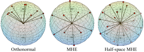
MHE faces different situations when it is applied to hidden layers and output layers. For hidden layers, applying MHE straightforwardly may still encourage some degree of redundancy since it will produce co-linear bases pointing to opposite directions (see Fig. 1 middle). In order to avoid such redundancy, we propose the half-space MHE which constructs a group of virtual neurons and minimize the hyperspherical energy of both existing and virtual neurons. For output layers, MHE aims to distribute the classifier neurons111Classifier neurons are the projection bases of the last layer (i.e., output layer) before input to softmax. as uniformly as possible to improve the inter-class feature separability. Different from MHE in hidden layers, classifier neurons should be distributed in the full space for the best classification performance [30, 29]. An intuitive comparison among the widely used orthonormal regularization, the proposed MHE and half-space MHE is provided in Fig. 1. One can observe that both MHE and half-space MHE are able to uniformly distribute the neurons over the hypersphere and half-space hypersphere, respectively. In contrast, conventional orthonormal regularization tends to group neurons closer, especially when the number of neurons is greater than the dimension.
MHE is originally defined on Euclidean distance, as indicated in Thomson problem. However, we further consider minimizing hyperspherical energy defined with respect to angular distance, which we will refer to as angular-MHE (A-MHE) in the following paper. In addition, we give some theoretical insights of MHE regularization, by discussing the asymptotic behavior and generalization error. Last, we apply MHE regularization to multiple vision tasks, including generic object recognition, class-imbalance learning, and face recognition. In the experiments, we show that MHE is architecture-agnostic and can considerably improve the generalization ability.
2 Related Works
Diversity regularization is shown useful in sparse coding [33, 36], ensemble learning [27, 25], self-paced learning [22], metric learning [60], etc. Early studies in sparse coding [33, 36] show that the generalization ability of codebook can be improved via diversity regularization, where the diversity is often modeled using the (empirical) covariance matrix. More recently, a series of studies have featured diversity regularization in neural networks [61, 59, 58, 5, 37, 57], where regularization is mostly achieved via promoting large angle/orthogonality, or reducing covariance between bases. Our work differs from these studies by formulating the diversity of neurons on the entire hypersphere, therefore promoting diversity from a more global, top-down perspective.
3 Learning Neurons towards Minimum Hyperspherical Energy
3.1 Formulation of Minimum Hyperspherical Energy
Minimum hyperspherical energy defines an equilibrium state of the configuration of neuron’s directions. We argue that the power of neural representation of each layer can be characterized by the hyperspherical energy of its neurons, and therefore a minimal energy configuration of neurons can induce better generalization. Before delving into details, we first define the hyperspherical energy functional for neurons (i.e., kernels) of -dimension as
| (1) |
where denotes Euclidean distance, is a decreasing real-valued function, and is the -th neuron weight projected onto the unit hypersphere . We also denote , and for short. There are plenty of choices for , but in this paper we use , known as Riesz -kernels. Particularly, as , , which is an affine transformation of . It follows that optimizing the logarithmic hyperspherical energy is essentially the limiting case of optimizing the hyperspherical energy . We therefore define for convenience.
The goal of the MHE criterion is to minimize the energy in Eq. (1) by varying the orientations of the neuron weights . To be precise, we solve an optimization problem: with . In particular, when , we solve the logarithmic energy minimization problem:
| (2) |
in which we essentially maximize the product of Euclidean distances. , and have interesting yet profound connections. Note that Thomson problem corresponds to minimizing , which is a NP-hard problem. Therefore in practice we can only compute its approximate solution by heuristics. In neural networks, such a differentiable objective can be directly optimized via gradient descent.
3.2 Logarithmic Hyperspherical Energy as a Relaxation
Optimizing the original energy in Eq. (1) is equivalent to optimizing its logarithmic form . To efficiently solve this difficult optimization problem, we can instead optimize the lower bound of as a surrogate energy, by applying Jensen’s inequality:
| (3) |
With , we observe that becomes , which is identical to the logarithmic hyperspherical energy up to a multiplicative factor . Therefore, minimizing can also be viewed as a relaxation of minimizing for .
3.3 MHE as Regularization for Neural Networks
Now that we have introduced the formulation of MHE, we propose MHE regularization for neural networks. In supervised neural network learning, the entire objective function is shown as follows:
| (4) |
where is the feature of the -th training sample entering the output layer, is the classifier neuron for the -th class in the output fully-connected layer and denotes its normalized version. denotes the hyperspherical energy for the neurons in the -th layer. is the number of classes, is the batch size, is the number of layers of the neural network, and is the number of neurons in the -th layer. denotes the hyperspherical energy of neurons . The weight decay is omitted here for simplicity, but we will use it in practice. An alternative interpretation of MHE regularization from a decoupled view is given in Section 3.7 and Appendix C. MHE has different effects and interpretations in regularizing hidden layers and output layers.
MHE for hidden layers. To make neurons in the hidden layers more discriminative and less redundant, we propose to use MHE as a form of regularization. MHE encourages the normalized neurons to be uniformly distributed on a unit hypersphere, which is partially inspired by the observation in [31] that angular difference in neurons preserves semantic (label-related) information. To some extent, MHE maximizes the average angular difference between neurons (specifically, the hyperspherical energy of neurons in every hidden layer). For instance, in CNNs we minimize the hyperspherical energy of kernels in convolutional and fully-connected layers except the output layer.
MHE for output layers. For the output layer, we propose to enhance the inter-class feature separability with MHE to learn discriminative and well-separated features. For classification tasks, MHE regularization is complementary to the softmax cross-entropy loss in CNNs. The softmax loss focuses more on the intra-class compactness, while MHE encourages the inter-class separability. Therefore, MHE on output layers can induce features with better generalization power.
3.4 MHE in Half Space
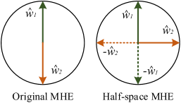
Directly applying the MHE formulation may still encounter some redundancy. An example in Fig. 2, with two neurons in a 2-dimensional space, illustrates this potential issue. Directly imposing the original MHE regularization leads to a solution that two neurons are collinear but with opposite directions. To avoid such redundancy, we propose the half-space MHE regularization which constructs some virtual neurons and minimizes the hyperspherical energy of both original and virtual neurons together. Specifically, half-space MHE constructs a collinear virtual neuron with opposite direction for every existing neuron. Therefore, we end up with minimizing the hyperspherical energy with neurons in the -th layer (i.e., minimizing ). This half-space variant will encourage the neurons to be less correlated and less redundant, as illustrated in Fig. 2. Note that, half-space MHE can only be used in hidden layers, because the collinear neurons do not constitute redundancy in output layers, as shown in [30]. Nevertheless, collinearity is usually not likely to happen in high-dimensional spaces, especially when the neurons are optimized to fit training data. This may be the reason that the original MHE regularization still consistently improves the baselines.
3.5 MHE beyond Euclidean Distance
The hyperspherical energy is originally defined based on the Euclidean distance on a hypersphere, which can be viewed as an angular measure. In addition to Euclidean distance, we further consider the geodesic distance on a unit hypersphere as a distance measure for neurons, which is exactly the same as the angle between neurons. Specifically, we consider to use to replace in hyperspherical energies. Following this idea, we propose angular MHE (A-MHE) as a simple extension, where the hyperspherical energy is rewritten as:
| (5) |
which can be viewed as redefining MHE based on geodesic distance on hyperspheres (i.e., angle), and can be used as an alternative to the original hyperspherical energy in Eq. (4). Note that, A-MHE can also be learned in full-space or half-space, leading to similar variants as original MHE. The key difference between MHE and A-MHE lies in the optimization dynamics, because their gradients w.r.t the neuron weights are quite different. A-MHE is also more computationally expensive than MHE.
3.6 Mini-batch Approximation for MHE
With a large number of neurons in one layer, calculating MHE can be computationally expensive as it requires computing the pair-wise distances between neurons. To address this issue, we propose the mini-batch version of MHE to approximate the MHE (either original or half-space) objective.
Mini-batch approximation for MHE on hidden layers. For hidden layers, mini-batch approximation iteratively takes a random batch of neurons as input and minimizes their hyperspherical energy as an approximation to the MHE. It can be viewed as dividing neurons into groups. Note that the gradient of the mini-batch objective is an unbiased estimation of the original gradient of MHE.
Data-dependent mini-batch approximation for output layers. For the output layer, the data-dependent mini-batch approximation iteratively takes the classifier neurons corresponding to the classes that appear in each mini-batch and minimize their hyperspherical energy. It minimizes in each iteration, where is the class label of the -th sample in each mini-batch, is the mini-batch size, and is the number of neurons (in a layer).
3.7 Discussions
Connections to scientific problems. The hyperspherical energy minimization has close relationships with scientific problems. When , Eq. (1) reduces to Thomson problem [49, 44] (in physics) where one needs to determine the minimum electrostatic potential energy configuration of mutually-repelling electrons on a unit sphere. When , Eq. (1) becomes Tammes problem [48] (in geometry) where the goal is to pack a given number of circles on the surface of a sphere such that the minimum distance between circles is maximized. When , Eq. (1) becomes Whyte’s problem where the goal is to maximize product of Euclidean distances as shown in Eq. (2). Our work aims to make use of important insights from these scientific problems to improve neural networks.
Understanding MHE from decoupled view. Inspired by decoupled networks [28], we can view the original convolution as the multiplication of the angular function and the magnitude function : where is the angle between the kernel and the input . From the equation above, we can see that the norm of the kernel and the direction (i.e., angle) of the kernel affect the inner product similarity differently. Typically, weight decay is to regularize the kernel by minimizing its norm, while there is no regularization on the direction of the kernel. Therefore, MHE completes this missing piece by promoting angular diversity. By combining MHE to a standard neural networks, the entire regularization term becomes
where , and are weighting hyperparameters for these three regularization terms. From the decoupled view, MHE makes a lot of senses in regularizing the neural networks, since it serves as a complementary and orthogonal role to weight decay. More discussions are in Appendix C.
Comparison to orthogonality/angle-promoting regularizations. Promoting orthogonality or large angles between bases has been a popular choice for encouraging diversity. Probably the most related and widely used one is the orthonormal regularization [31] which aims to minimize , where denotes the weights of a group of neurons with each column being one neuron and is an identity matrix. One similar regularization is the orthogonality regularization [37] which minimizes the sum of the cosine values between all the kernel weights. These methods encourage kernels to be orthogonal to each other, while MHE does not. Instead, MHE encourages the hyperspherical diversity among these kernels, and these kernels are not necessarily orthogonal to each other. [58] proposes the angular constraint which aims to constrain the angles between different kernels of the neural network, but quite different from MHE, they use a hard constraint to impose this angular regularization. Moreover, these methods model diversity regularization at a more local level, while MHE regularization seeks to model the problem in a more top-down manner.
Normalized neurons in MHE. From Eq. 1, one can see that the normalized neurons are used to compute MHE, because we aim to encourage the diversity on a hypersphere. However, a natural question may arise: what if we use the original (i.e., unnormalized) neurons to compute MHE? First, combining the norm of kernels (i.e., neurons) into MHE may lead to a trivial gradient descent direction: simply increasing the norm of all kernels. Suppose all kernel directions stay unchanged, increasing the norm of all kernels by a factor can effectively decrease the objective value of MHE. Second, coupling the norm of kernels into MHE may contradict with weight decay which aims to decrease the norm of kernels. Moreover, normalized neurons imply that the importance of all neurons is the same, which matches the intuition in [29, 31, 28]. If we desire different importance for different neurons, we can also manually assign a fixed weight for each neuron. This may be useful when we have already known certain neurons are more important and we want them to be relatively fixed. The neuron with large weight tends to be updated less. We will discuss it more in Appendix D.
4 Theoretical Insights
This section leverages a number of rigorous theoretical results from [39, 24, 13, 26, 12, 24, 8, 56] and provides theoretical yet intuitive understandings about MHE.
4.1 Asymptotic Behavior
This subsection shows how the hyperspherical energy behaves asymptotically. Specifically, as , we can show that the solution tends to be uniformly distributed on hypersphere when the hyperspherical energy defined in Eq. (1) achieves its minimum.
Definition 1 (minimal hyperspherical -energy).
We define the minimal -energy for points on the unit hypersphere as
| (6) |
where the infimum is taken over all possible on . Any configuration of to attain the infimum is called an -extremal configuration. Usually if is greater than and if .
We discuss the asymptotic behavior () in three cases: , , and . We first write the energy integral as which is taken over all probability measure supported on . With , is minimal when is the spherical measure on , where denotes the -dimensional Hausdorff measure. When , becomes infinity, which therefore requires different analysis. In general, we can say all -extremal configurations asymptotically converge to uniform distribution on a hypersphere, as stated in Theorem 1. This asymptotic behavior has been heavily studied in [39, 24, 13].
Theorem 1 (asymptotic uniform distribution on hypersphere).
Any sequence of optimal -energy configurations is asymptotically uniformly distributed on in the sense of the weak-star topology of measures, namely
| (7) |
where denotes the unit point mass at , and is the spherical measure on .
Theorem 2 (asymptotics of the minimal hyperspherical -energy).
We have that exists for the minimal -energy. For , . For , . For , . Particularly if , we have .
Theorem 2 tells us the growth power of the minimal hyperspherical -energy when goes to infinity. Therefore, different potential power leads to different optimization dynamics. In the light of the behavior of the energy integral, MHE regularization will focus more on local influence from neighborhood neurons instead of global influences from all the neurons as the power increases.
4.2 Generalization and Optimization
As proved in [56], in one-hidden-layer neural network, the diversity of neurons can effectively eliminate the spurious local minima despite the non-convexity in learning dynamics of neural networks. Following such an argument, our MHE regularization, which encourages the diversity of neurons, naturally matches the theoretical intuition in [56], and effectively promotes the generalization of neural networks. While hyperspherical energy is minimized such that neurons become diverse on hyperspheres, the hyperspherical diversity is closely related to the generalization error.
More specifically, in a one-hidden-layer neural network with least squares loss , we can compute its gradient w.r.t as . ( is the nonlinear activation function and is its subgradient. is the training sample. denotes the weights of hidden layer and is the weights of output layer.) Subsequently, we can rewrite this gradient as a matrix form: where and . Further, we can obtain the inequality . is actually the training error. To make the training error small, we need to lower bound away from zero. From [56, 3], one can know that the lower bound of is directly related to the hyperspherical diversity of neurons. After bounding the training error, it is easy to bound the generalization error using Rademachar complexity.
5 Applications and Experiments
5.1 Improving Network Generalization
First, we perform ablation study and some exploratory experiments on MHE. Then we apply MHE to large-scale object recognition and class-imbalance learning. For all the experiments on CIFAR-10 and CIFAR-100 in the paper, we use moderate data augmentation, following [15, 28]. For ImageNet-2012, we follow the same data augmentation in [31]. We train all the networks using SGD with momentum , and the network initialization follows [14]. All the networks use BN [21] and ReLU if not otherwise specified. Experimental details are given in each subsection and Appendix A.
5.1.1 Ablation Study and Exploratory Experiments
| Method | CIFAR-10 | CIFAR-100 | ||||
| MHE | 6.22 | 6.74 | 6.44 | 27.15 | 27.09 | 26.16 |
| Half-space MHE | 6.28 | 6.54 | 6.30 | 25.61 | 26.30 | 26.18 |
| A-MHE | 6.21 | 6.77 | 6.45 | 26.17 | 27.31 | 27.90 |
| Half-space A-MHE | 6.52 | 6.49 | 6.44 | 26.03 | 26.52 | 26.47 |
| Baseline | 7.75 | 28.13 | ||||
Variants of MHE. We evaluate all different variants of MHE on CIFAR-10 and CIFAR-100, including original MHE (with the power ) and half-space MHE (with the power ) with both Euclidean and angular distance. In this experiment, all methods use CNN-9 (see Appendix A). The results in Table 1 show that all the variants of MHE perform consistently better than the baseline. Specifically, the half-space MHE has more significant performance gain compared to the other MHE variants, and MHE with Euclidean and angular distance perform similarly. In general, MHE with performs best among . In the following experiments, we use and Euclidean distance for both MHE and half-space MHE by default if not otherwise specified.
| Method | 16/32/64 | 32/64/128 | 64/128/256 | 128/256/512 | 256/512/1024 |
| Baseline | 47.72 | 38.64 | 28.13 | 24.95 | 25.45 |
| MHE | 36.84 | 30.05 | 26.75 | 24.05 | 23.14 |
| Half-space MHE | 35.16 | 29.33 | 25.96 | 23.38 | 21.83 |
Network width. We evaluate MHE with different network width. We use CNN-9 as our base network, and change its filter number in Conv1.x, Conv2.x and Conv3.x (see Appendix A) to 16/32/64, 32/64/128, 64/128/256, 128/256/512 and 256/512/1024. Results in Table 2 show that both MHE and half-space MHE consistently outperform the baseline, showing stronger generalization. Interestingly, both MHE and half-space MHE have more significant gain while the filter number is smaller in each layer, indicating that MHE can help the network to make better use of the neurons. In general, half-space MHE performs consistently better than MHE, showing the necessity of reducing collinearity redundancy among neurons. Both MHE and half-space MHE outperform the baseline with a huge margin while the network is either very wide or very narrow, showing the superiority in improving generalization.
| Method | CNN-6 | CNN-9 | CNN-15 |
| Baseline | 32.08 | 28.13 | N/C |
| MHE | 28.16 | 26.75 | 26.9 |
| Half-space MHE | 27.56 | 25.96 | 25.84 |
Network depth. We perform experiments with different network depth to better evaluate the performance of MHE. We fix the filter number in Conv1.x, Conv2.x and Conv3.x to 64, 128 and 256, respectively. We compare 6-layer CNN, 9-layer CNN and 15-layer CNN. The results are given in Table 3. Both MHE and half-space MHE perform significantly better than the baseline. More interestingly, baseline CNN-15 can not converge, while CNN-15 is able to converge reasonably well if we use MHE to regularize the network. Moreover, we also see that half-space MHE can consistently show better generalization than MHE with different network depth.
| Method | H O | H O | H O |
| MHE | 26.85 | 26.55 | 26.16 |
| Half-space MHE | N/A | 26.28 | 25.61 |
| A-MHE | 27.8 | 26.56 | 26.17 |
| Half-space A-MHE | N/A | 26.64 | 26.03 |
| Baseline | 28.13 | ||
Ablation study. Since the current MHE regularizes the neurons in the hidden layers and the output layer simultaneously, we perform ablation study for MHE to further investigate where the gain comes from. This experiment uses the CNN-9. The results are given in Table 4. “H” means that we apply MHE to all the hidden layers, while “O” means that we apply MHE to the output layer. Because the half-space MHE can not be applied to the output layer, so there is “N/A” in the table. In general, we find that applying MHE to both the hidden layers and the output layer yields the best performance, and using MHE in the hidden layers usually produces better accuracy than using MHE in the output layer.
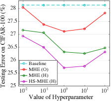
Hyperparameter experiment. We evaluate how the selection of hyperparameter affects the performance. We experiment with different hyperparameters from to on CIFAR-100 with the CNN-9. HS-MHE denotes the half-space MHE. We evaluate MHE variants by separately applying MHE to the output layer (“O”), MHE to the hidden layers (“H”), and the half-space MHE to the hidden layers (“H”). The results in Fig. 3 show that our MHE is not very hyperparameter-sensitive and can consistently beat the baseline by a considerable margin. One can observe that MHE’s hyperparameter works well from to and therefore is easy to set. In contrast, the hyperparameter of weight decay could be more sensitive than MHE. Half-space MHE can consistently outperform the original MHE under all different hyperparameter settings. Interestingly, applying MHE only to hidden layers can achieve better accuracy than applying MHE only to output layers.
| Method | CIFAR-10 | CIFAR-100 |
| ResNet-110-original [15] | 6.61 | 25.16 |
| ResNet-1001 [16] | 4.92 | 22.71 |
| ResNet-1001 (64 batch) [16] | 4.64 | - |
| baseline | 5.19 | 22.87 |
| MHE | 4.72 | 22.19 |
| Half-space MHE | 4.66 | 22.04 |
MHE for ResNets. Besides the standard CNN, we also evaluate MHE on ResNet-32 to show that our MHE is architecture-agnostic and can improve accuracy on multiple types of architectures. Besides ResNets, MHE can also be applied to GoogleNet [47], SphereNets [31] (the experimental results are given in Appendix E), DenseNet [18], etc. Detailed architecture settings are given in Appendix A. The results on CIFAR-10 and CIFAR-100 are given in Table 5. One can observe that applying MHE to ResNet also achieves considerable improvements, showing that MHE is generally useful for different architectures. Most importantly, adding MHE regularization will not affect the original architecture settings, and it can readily improve the network generalization at a neglectable computational cost.
5.1.2 Large-scale Object Recognition
| Method | ResNet-18 | ResNet-34 |
| baseline | 32.95 | 30.04 |
| Orthogonal [37] | 32.65 | 29.74 |
| Orthonormal | 32.61 | 29.75 |
| MHE | 32.50 | 29.60 |
| Half-space MHE | 32.45 | 29.50 |
We evaluate MHE on large-scale ImageNet-2012 datasets. Specifically, we perform experiment using ResNets, and then report the top-1 validation error (center crop) in Table 6. From the results, we still observe that both MHE and half-space MHE yield consistently better recognition accuracy than the baseline and the orthonormal regularization (after tuning its hyperparameter). To better evaluate the consistency of MHE’s performance gain, we use two ResNets with different depth: ResNet-18 and ResNet-34. On these two different networks, both MHE and half-space MHE outperform the baseline by a significant margin, showing consistently better generalization power. Moreover, half-space MHE performs slightly better than full-space MHE as expected.
5.1.3 Class-imbalance Learning
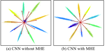
Because MHE aims to maximize the hyperspherical margin between different classifier neurons in the output layer, we can naturally apply MHE to class-imbalance learning where the number of training samples in different classes is imbalanced. We demonstrate the power of MHE in class-imbalance learning through a toy experiment. We first randomly throw away 98% training data for digit 0 in MNIST (only 100 samples are preserved for digit 0), and then train a 6-layer CNN on this imbalance MNIST. To visualize the learned features, we set the output feature dimension as 2. The features and classifier neurons on the full training set are visualized in Fig. 4 where each color denotes a digit and red arrows are the normalized classifier neurons. Although we train the network on the imbalanced training set, we visualize the features of the full training set for better demonstration. The visualization for the full testing set is also given in Appendix H. From Fig. 4, one can see that the CNN without MHE tends to ignore the imbalanced class (digit 0) and the learned classifier neuron is highly biased to another digit. In contrast, the CNN with MHE can learn reasonably separable distribution even if digit 0 only has 2% samples compared to the other classes. Using MHE in this toy setting can readily improve the accuracy on the full testing set from to . Most importantly, the classifier neuron for digit 0 is also properly learned, similar to the one learned on the balanced dataset. Note that, half-space MHE can not be applied to the classifier neurons, because the classifier neurons usually need to occupy the full feature space.
| Method | Single | Err. (S) | Multiple |
| Baseline | 9.80 | 30.40 | 12.00 |
| Orthonormal | 8.34 | 26.80 | 10.80 |
| MHE | 7.98 | 25.80 | 10.25 |
| Half-space MHE | 7.90 | 26.40 | 9.59 |
| A-MHE | 7.96 | 26.00 | 9.88 |
| Half-space A-MHE | 7.59 | 25.90 | 9.89 |
We experiment MHE in two data imbalance settings on CIFAR-10: 1) single class imbalance (S) - All classes have the same number of images but one single class has significantly less number, and 2) multiple class imbalance (M) - The number of images decreases as the class index decreases from 9 to 0. We use CNN-9 for all the compared regularizations. Detailed setups are provided in Appendix A. In Table 7, we report the error rate on the whole testing set. In addition, we report the error rate (denoted by Err. (S)) on the imbalance class (single imbalance setting) in the full testing set. From the results, one can observe that CNN-9 with MHE is able to effectively perform recognition when classes are imbalanced. Even only given a small portion of training data in a few classes, CNN-9 with MHE can achieve very competitive accuracy on the full testing set, showing MHE’s superior generalization power. Moreover, we also provide experimental results on imbalanced CIFAR-100 in Appendix H.
5.2 SphereFace+: Improving Inter-class Feature Separability via MHE for Face Recognition
We have shown that full-space MHE for output layers can encourage classifier neurons to distribute more evenly on hypersphere and therefore improve inter-class feature separability. Intuitively, the classifier neurons serve as the approximate center for features from each class, and can therefore guide the feature learning. We also observe that open-set face recognition (e.g., face verification) requires the feature centers to be as separable as possible [29]. This connection inspires us to apply MHE to face recognition. Specifically, we propose SphereFace+ by applying MHE to SphereFace [29]. The objective of SphereFace, angular softmax loss () that encourages intra-class feature compactness, is naturally complementary to that of MHE. The objective function of SphereFace+ is defined as
| (8) |
where is the number of classes, is the mini-batch size, is the number of classifier neurons, the deep feature of the -th face ( is its groundtruth label), and is the -th classifier neuron. is a hyperparameter for SphereFace, controlling the degree of intra-class feature compactness (i.e., the size of the angular margin). Because face datesets usually have thousands of identities, we will use the data-dependent mini-batch approximation MHE as shown in Eq. (8) in the output layer to reduce computational cost. MHE completes a missing piece for SphereFace by promoting the inter-class separability. SphereFace+ consistently outperforms SphereFace, and achieves state-of-the-art performance on both LFW [19] and MegaFace [23] datasets. More results on MegaFace are put in Appendix I. More evaluations and results can be found in Appendix F and Appendix J.
| LFW | MegaFace | |||
| SphereFace | SphereFace+ | SphereFace | SphereFace+ | |
| 96.35 | 97.15 | 39.12 | 45.90 | |
| 98.87 | 99.05 | 60.48 | 68.51 | |
| 98.97 | 99.13 | 63.71 | 66.89 | |
| 99.26 | 99.32 | 70.68 | 71.30 | |
| LFW | MegaFace | |||
| SphereFace | SphereFace+ | SphereFace | SphereFace+ | |
| 96.93 | 97.47 | 41.07 | 45.55 | |
| 99.03 | 99.22 | 62.01 | 67.07 | |
| 99.25 | 99.35 | 69.69 | 70.89 | |
| 99.42 | 99.47 | 72.72 | 73.03 | |
Performance under different . We evaluate SphereFace+ with two different architectures (SphereFace-20 and SphereFace-64) proposed in [29]. Specifically, SphereFace-20 and SphereFace-64 are 20-layer and 64-layer modified residual networks, respectively. We train our network with the publicly available CASIA-Webface dataset [62], and then test the learned model on LFW and MegaFace dataset. In MegaFace dataset, the reported accuracy indicates rank-1 identification accuracy with 1 million distractors. All the results in Table 5.2 and Table 5.2 are computed without model ensemble and PCA. One can observe that SphereFace+ consistently outperforms SphereFace by a considerable margin on both LFW and MegaFace datasets under all different settings of . Moreover, the performance gain generalizes across network architectures with different depth.
| Method | LFW | MegaFace |
| Softmax Loss | 97.88 | 54.86 |
| Softmax+Contrastive [46] | 98.78 | 65.22 |
| Triplet Loss [41] | 98.70 | 64.80 |
| L-Softmax Loss [30] | 99.10 | 67.13 |
| Softmax+Center Loss [55] | 99.05 | 65.49 |
| CosineFace [53, 51] | 99.10 | 75.10 |
| SphereFace | 99.42 | 72.72 |
| SphereFace+ (ours) | 99.47 | 73.03 |
Comparison to state-of-the-art methods. We also compare our methods with some widely used loss functions. All these compared methods use SphereFace-64 network that are trained with CASIA dataset. All the results are given in Table 10 computed without model ensemble and PCA. Compared to the other state-of-the-art methods, SphereFace+ achieves the best accuracy on LFW dataset, while being comparable to the best accuracy on MegaFace dataset. Current state-of-the-art face recognition methods [51, 29, 53, 6, 32] usually only focus on compressing the intra-class features, which makes MHE a potentially useful tool in order to further improve these face recognition methods.
6 Concluding Remarks
We borrow some useful ideas and insights from physics and propose a novel regularization method for neural networks, called minimum hyperspherical energy (MHE), to encourage the angular diversity of neuron weights. MHE can be easily applied to every layer of a neural network as a plug-in regularization, without modifying the original network architecture. Different from existing methods, such diversity can be viewed as uniform distribution over a hypersphere. In this paper, MHE has been specifically used to improve network generalization for generic image classification, class-imbalance learning and large-scale face recognition, showing consistent improvements in all tasks. Moreover, MHE can significantly improve the image generation quality of GANs (see Appendix G). In summary, our paper casts a novel view on regularizing the neurons by introducing hyperspherical diversity.
Acknowledgements
This project was supported in part by NSF IIS-1218749, NIH BIGDATA 1R01GM108341, NSF CAREER IIS-1350983, NSF IIS-1639792 EAGER, NSF IIS-1841351 EAGER, NSF CCF-1836822, NSF CNS-1704701, ONR N00014-15-1-2340, Intel ISTC, NVIDIA, Amazon AWS and Siemens. We would like to thank NVIDIA corporation for donating Titan Xp GPUs to support our research. We also thank Tuo Zhao for the valuable discussions and suggestions.
References
- [1] Alireza Aghasi, Nam Nguyen, and Justin Romberg. Net-trim: A layer-wise convex pruning of deep neural networks. In NIPS, 2017.
- [2] Jimmy Lei Ba, Jamie Ryan Kiros, and Geoffrey E Hinton. Layer normalization. arXiv preprint arXiv:1607.06450, 2016.
- [3] Dmitriy Bilyk and Michael T Lacey. One-bit sensing, discrepancy and stolarsky’s principle. Sbornik: Mathematics, 208(6):744, 2017.
- [4] Andrew Brock, Theodore Lim, James M Ritchie, and Nick Weston. Neural photo editing with introspective adversarial networks. In ICLR, 2017.
- [5] Michael Cogswell, Faruk Ahmed, Ross Girshick, Larry Zitnick, and Dhruv Batra. Reducing overfitting in deep networks by decorrelating representations. In ICLR, 2016.
- [6] Jiankang Deng, Jia Guo, and Stefanos Zafeiriou. Arcface: Additive angular margin loss for deep face recognition. arXiv preprint arXiv:1801.07698, 2018.
- [7] Ian Goodfellow, Jean Pouget-Abadie, Mehdi Mirza, Bing Xu, David Warde-Farley, Sherjil Ozair, Aaron Courville, and Yoshua Bengio. Generative adversarial nets. In NIPS, 2014.
- [8] Mario Götz and Edward B Saff. Note on d—extremal configurations for the sphere in r d+1. In Recent Progress in Multivariate Approximation, pages 159–162. Springer, 2001.
- [9] Ishaan Gulrajani, Faruk Ahmed, Martin Arjovsky, Vincent Dumoulin, and Aaron C Courville. Improved training of wasserstein gans. In NIPS, 2017.
- [10] Yandong Guo, Lei Zhang, Yuxiao Hu, Xiaodong He, and Jianfeng Gao. Ms-celeb-1m: A dataset and benchmark for large-scale face recognition. In ECCV, 2016.
- [11] Song Han, Huizi Mao, and William J Dally. Deep compression: Compressing deep neural networks with pruning, trained quantization and huffman coding. In ICLR, 2016.
- [12] DP Hardin and EB Saff. Minimal riesz energy point configurations for rectifiable d-dimensional manifolds. arXiv preprint math-ph/0311024, 2003.
- [13] DP Hardin and EB Saff. Discretizing manifolds via minimum energy points. Notices of the AMS, 51(10):1186–1194, 2004.
- [14] Kaiming He, Xiangyu Zhang, Shaoqing Ren, and Jian Sun. Delving deep into rectifiers: Surpassing human-level performance on imagenet classification. In ICCV, 2015.
- [15] Kaiming He, Xiangyu Zhang, Shaoqing Ren, and Jian Sun. Deep residual learning for image recognition. In CVPR, 2016.
- [16] Kaiming He, Xiangyu Zhang, Shaoqing Ren, and Jian Sun. Identity mappings in deep residual networks. In ECCV, 2016.
- [17] Andrew G Howard, Menglong Zhu, Bo Chen, Dmitry Kalenichenko, Weijun Wang, Tobias Weyand, Marco Andreetto, and Hartwig Adam. Mobilenets: Efficient convolutional neural networks for mobile vision applications. arXiv preprint arXiv:1704.04861, 2017.
- [18] Gao Huang, Zhuang Liu, Laurens Van Der Maaten, and Kilian Q Weinberger. Densely connected convolutional networks. In CVPR, 2017.
- [19] Gary B Huang, Manu Ramesh, Tamara Berg, and Erik Learned-Miller. Labeled faces in the wild: A database for studying face recognition in unconstrained environments. Technical report, Technical Report, 2007.
- [20] Forrest N Iandola, Song Han, Matthew W Moskewicz, Khalid Ashraf, William J Dally, and Kurt Keutzer. Squeezenet: Alexnet-level accuracy with 50x fewer parameters and< 0.5 mb model size. arXiv preprint arXiv:1602.07360, 2016.
- [21] Sergey Ioffe and Christian Szegedy. Batch normalization: Accelerating deep network training by reducing internal covariate shift. In ICML, 2015.
- [22] Lu Jiang, Deyu Meng, Shoou-I Yu, Zhenzhong Lan, Shiguang Shan, and Alexander Hauptmann. Self-paced learning with diversity. In NIPS, 2014.
- [23] Ira Kemelmacher-Shlizerman, Steven M Seitz, Daniel Miller, and Evan Brossard. The megaface benchmark: 1 million faces for recognition at scale. In CVPR, 2016.
- [24] Arno Kuijlaars and E Saff. Asymptotics for minimal discrete energy on the sphere. Transactions of the American Mathematical Society, 350(2):523–538, 1998.
- [25] Ludmila I Kuncheva and Christopher J Whitaker. Measures of diversity in classifier ensembles and their relationship with the ensemble accuracy. Machine learning, 51(2):181–207, 2003.
- [26] Naum Samouilovich Landkof. Foundations of modern potential theory, volume 180. Springer, 1972.
- [27] Nan Li, Yang Yu, and Zhi-Hua Zhou. Diversity regularized ensemble pruning. In Joint European Conference on Machine Learning and Knowledge Discovery in Databases, 2012.
- [28] Weiyang Liu, Zhen Liu, Zhiding Yu, Bo Dai, Rongmei Lin, Yisen Wang, James M Rehg, and Le Song. Decoupled networks. CVPR, 2018.
- [29] Weiyang Liu, Yandong Wen, Zhiding Yu, Ming Li, Bhiksha Raj, and Le Song. Sphereface: Deep hypersphere embedding for face recognition. In CVPR, 2017.
- [30] Weiyang Liu, Yandong Wen, Zhiding Yu, and Meng Yang. Large-margin softmax loss for convolutional neural networks. In ICML, 2016.
- [31] Weiyang Liu, Yan-Ming Zhang, Xingguo Li, Zhiding Yu, Bo Dai, Tuo Zhao, and Le Song. Deep hyperspherical learning. In NIPS, 2017.
- [32] Yu Liu, Hongyang Li, and Xiaogang Wang. Rethinking feature discrimination and polymerization for large-scale recognition. arXiv preprint arXiv:1710.00870, 2017.
- [33] Julien Mairal, Francis Bach, Jean Ponce, and Guillermo Sapiro. Online dictionary learning for sparse coding. In ICML, 2009.
- [34] Dmytro Mishkin and Jiri Matas. All you need is a good init. In ICLR, 2016.
- [35] Takeru Miyato, Toshiki Kataoka, Masanori Koyama, and Yuichi Yoshida. Spectral normalization for generative adversarial networks. In ICLR, 2018.
- [36] Ignacio Ramirez, Pablo Sprechmann, and Guillermo Sapiro. Classification and clustering via dictionary learning with structured incoherence and shared features. In CVPR, 2010.
- [37] Pau Rodríguez, Jordi Gonzalez, Guillem Cucurull, Josep M Gonfaus, and Xavier Roca. Regularizing cnns with locally constrained decorrelations. In ICLR, 2017.
- [38] Aruni RoyChowdhury, Prakhar Sharma, Erik Learned-Miller, and Aruni Roy. Reducing duplicate filters in deep neural networks. In NIPS workshop on Deep Learning: Bridging Theory and Practice, 2017.
- [39] Edward B Saff and Amo BJ Kuijlaars. Distributing many points on a sphere. The mathematical intelligencer, 19(1):5–11, 1997.
- [40] Tim Salimans and Diederik P Kingma. Weight normalization: A simple reparameterization to accelerate training of deep neural networks. In NIPS, 2016.
- [41] Florian Schroff, Dmitry Kalenichenko, and James Philbin. Facenet: A unified embedding for face recognition and clustering. In CVPR, 2015.
- [42] Wenling Shang, Kihyuk Sohn, Diogo Almeida, and Honglak Lee. Understanding and improving convolutional neural networks via concatenated rectified linear units. In ICML, 2016.
- [43] Karen Simonyan and Andrew Zisserman. Very deep convolutional networks for large-scale image recognition. arXiv:1409.1556, 2014.
- [44] Steve Smale. Mathematical problems for the next century. The mathematical intelligencer, 20(2):7–15, 1998.
- [45] Nitish Srivastava, Geoffrey Hinton, Alex Krizhevsky, Ilya Sutskever, and Ruslan Salakhutdinov. Dropout: A simple way to prevent neural networks from overfitting. JMLR, 15(1):1929–1958, 2014.
- [46] Yi Sun, Xiaogang Wang, and Xiaoou Tang. Deep learning face representation from predicting 10,000 classes. In CVPR, 2014.
- [47] Christian Szegedy, Wei Liu, Yangqing Jia, Pierre Sermanet, Scott Reed, Dragomir Anguelov, Dumitru Erhan, Vincent Vanhoucke, and Andrew Rabinovich. Going deeper with convolutions. In CVPR, 2015.
- [48] Pieter Merkus Lambertus Tammes. On the origin of number and arrangement of the places of exit on the surface of pollen-grains. Recueil des travaux botaniques néerlandais, 27(1):1–84, 1930.
- [49] Joseph John Thomson. Xxiv. on the structure of the atom: an investigation of the stability and periods of oscillation of a number of corpuscles arranged at equal intervals around the circumference of a circle; with application of the results to the theory of atomic structure. The London, Edinburgh, and Dublin Philosophical Magazine and Journal of Science, 7(39):237–265, 1904.
- [50] Fei Wang, Liren Chen, Cheng Li, Shiyao Huang, Yanjie Chen, Chen Qian, and Chen Change Loy. The devil of face recognition is in the noise. In ECCV, 2018.
- [51] Feng Wang, Weiyang Liu, Haijun Liu, and Jian Cheng. Additive margin softmax for face verification. arXiv preprint arXiv:1801.05599, 2018.
- [52] Feng Wang, Xiang Xiang, Jian Cheng, and Alan L Yuille. Normface: L2 hypersphere embedding for face verification. arXiv preprint arXiv:1704.06369, 2017.
- [53] Hao Wang, Yitong Wang, Zheng Zhou, Xing Ji, Zhifeng Li, Dihong Gong, Jingchao Zhou, and Wei Liu. Cosface: Large margin cosine loss for deep face recognition. arXiv preprint arXiv:1801.09414, 2018.
- [54] David Warde-Farley and Yoshua Bengio. Improving generative adversarial networks with denoising feature matching. In ICLR, 2017.
- [55] Yandong Wen, Kaipeng Zhang, Zhifeng Li, and Yu Qiao. A discriminative feature learning approach for deep face recognition. In ECCV, 2016.
- [56] Bo Xie, Yingyu Liang, and Le Song. Diverse neural network learns true target functions. arXiv preprint arXiv:1611.03131, 2016.
- [57] Di Xie, Jiang Xiong, and Shiliang Pu. All you need is beyond a good init: Exploring better solution for training extremely deep convolutional neural networks with orthonormality and modulation. arXiv:1703.01827, 2017.
- [58] Pengtao Xie, Yuntian Deng, Yi Zhou, Abhimanu Kumar, Yaoliang Yu, James Zou, and Eric P Xing. Learning latent space models with angular constraints. In ICML, 2017.
- [59] Pengtao Xie, Aarti Singh, and Eric P Xing. Uncorrelation and evenness: a new diversity-promoting regularizer. In ICML, 2017.
- [60] Pengtao Xie, Wei Wu, Yichen Zhu, and Eric P Xing. Orthogonality-promoting distance metric learning: convex relaxation and theoretical analysis. In ICML, 2018.
- [61] Pengtao Xie, Jun Zhu, and Eric Xing. Diversity-promoting bayesian learning of latent variable models. In ICML, 2016.
- [62] Dong Yi, Zhen Lei, Shengcai Liao, and Stan Z Li. Learning face representation from scratch. arXiv:1411.7923, 2014.
- [63] Kaipeng Zhang, Zhanpeng Zhang, Zhifeng Li, and Yu Qiao. Joint face detection and alignment using multitask cascaded convolutional networks. IEEE Signal Processing Letters, 23(10):1499–1503, 2016.
- [64] Xiangyu Zhang, Xinyu Zhou, Mengxiao Lin, and Jian Sun. Shufflenet: An extremely efficient convolutional neural network for mobile devices. arXiv preprint arXiv:1707.01083, 2017.
Appendix
Appendix A Experimental Details
| Layer | CNN-6 | CNN-9 | CNN-15 |
| Conv1.x | [33, 64]2 | [33, 64]3 | [33, 64]5 |
| Pool1 | 22 Max Pooling, Stride 2 | ||
| Conv2.x | [33, 128]2 | [33, 128]3 | [33, 128]5 |
| Pool2 | 22 Max Pooling, Stride 2 | ||
| Conv3.x | [33, 256]2 | [33, 256]3 | [33, 256]5 |
| Pool3 | 22 Max Pooling, Stride 2 | ||
| Fully Connected | 256 | 256 | 256 |
| Layer | ResNet-32 for CIFAR-10/100 | ResNet-18 for ImageNet-2012 | ResNet-34 for ImageNet-2012 | ||||
| Conv0.x | N/A |
|
|
||||
| Conv1.x |
|
||||||
| Conv2.x |
|
||||||
| Conv3.x |
|
||||||
| Conv4.x | N/A | ||||||
| Average Pooling | |||||||
General settings. The network architectures used in the paper are elaborated in Table 11 Table 12. For CIFAR-10 and CIFAR-100, we use batch size 128. We start with learning rate 0.1, divide it by 10 at 20k, 30k and 37.5k iterations, and terminate training at 42.5k iterations. For ImageNet-2012, we use batch size 64 and start with learning rate 0.1. The learning rate is divided by 10 at 150k, 300k and 400k iterations, and the training is terminated at 500k iterations. Note that, for all the compared methods, we always use the best possible hyperparameters to make sure that the comparison is fair. The baseline has exactly the same architecture and training settings as the one that MHE uses, and the only difference is an additional MHE regularization. For full-space MHE in hidden layers, we set as for all experiments. For half-space MHE in hidden layers, we set as for all experiments. For MHE in output layers, we set as for all experiments. We use for the orthonormal regularization. If not otherwise specified, standard weight decay () is applied to all the neural network including baselines and the networks that use MHE regularization. A very minor issue for the hyperparameters is that it may increase as the number of layers increases, so we can potentially further divide the hyperspherical energy for the hidden layers by the number of layers. It will probably change the current optimal hyperparameter setting by a constant multiplier. For notation simplicity, we do not explicitly write out the weight decay term in the loss function in the main paper. Note that, all the neuron weights in the neural networks used in the paper are not normalized (unless otherwise specified), but the MHE will normalize the neuron weights while computing the regularization loss. As a result, MHE does not need to modify any component of the original neural networks, and it can simply be viewed as an extra regularization loss that can boost the performance. Because half-space variants can only applied to the hidden layers, both original MHE and its half-space version apply the full-space MHE to the output layer by default. The difference between MHE and half-space MHE are only in the regularization for the hidden layers.
Class-imbalance learning. There are 50000 training images in the original CIFAR-10 dataset, with 5000 images per class. For the single class imbalance setting, we keep original images of class 1-9 and randomly throw away 90% images of class 0. The total number of training images in this setting is 45500. For the multiple class imbalance setting, we set the number of each class equals to . For instance, class 0 has 500 images, class 1 has 1000 images and class 9 has 5000 images. The total number of training images in this setting is 27500. Note that, both half-space MHE and half-space A-MHE in Table 7 and Table 8 mean that the half-space variants have been applied to the hidden layers. For the output layer (i.e., classifier neurons), only full-space MHE can be used.
SphereFace+. SphereFace+ uses the same face detection and alignment method [63] as SphereFace [29]. The testing protocol on LFW and MegaFace is also the same as SphereFace. We use exactly the same preprocessing as in the SphereFace repository. Detailed network architecture settings of SphereFace-20 and SphereFace-64 can be found in [29]. Specifically, we use full-space MHE with Euclidean distance and in the output layer. Essentially, we treat MHE as an additional loss function which aims to enlarge the inter-class angular distance of features and serves a complementary role to the angular softmax in SphereFace. Note that, for the results of CosineFace [53], we directly use the results (with the same training settings and without using feature normalization) reported in the paper. Since ours also does not perform feature normalization, it is a fair comparison. With feature normalization, we find that the performance of SphereFace+ will also be improved significantly. However, feature normalization makes the results more tricky, because it will involve another hyperparameter that controls the projection radius of feature normalization.
In order to reduce the training difficulty, we adopt a new training strategy. Specifically, we first train a model using the original SphereFace, and then use the new loss function proposed in Eq. 8 to finetune the pretrained SphereFace model. Note that, only the results for face recognition are obtained using this training strategy.
Appendix B Proof of Theorem 1 and Theorem 2
Theorem 1 and Theorem 2 are natural results from classic potential theory [26] and spherical configuration [12, 24, 8]. We discuss the asymptotic behavior () in three cases: , , and . We first write the energy integral as
| (9) |
which is taken over all probability measure supported on . With , is minimal when is the spherical measure on , where denotes the -dimensional Hausdorff measure. When , becomes infinity, which therefore requires different analysis.
First, the classic potential theory [26] can directly give the following results for the case where :
Lemma 1.
If ,
| (10) |
where is defined in the main paper. Moreover, any sequence of optimal hyperspherical -energy configurations is asymptotically uniformly distributed in the sense that for the weak-star topology measures,
| (11) |
where denotes the unit point mass at , and is the spherical measure on .
Lemma 2.
Let be the closed unit ball in . For ,
| (12) |
and any sequence of optimal -energy configurations satisfies Eq. 11.
which concludes the case of . Therefore, we are left with the case where . For this case, we can use the results from [12]:
Lemma 3.
Let be compact with , and be a sequence of asymptotically optimal -point configurations in in the sense that for some ,
| (13) |
or
| (14) |
where is a finite positive constant independent of . Let be the unit point mass at the point . Then in the weak-star topology of measures we have
| (15) |
Appendix C Understanding MHE from Decoupled View
Inspired by decoupled networks [28], we can view the original convolution as the multiplication of the angular function and the magnitude function :
| (16) | ||||
where is the angle between the kernel and the input . From the equation above, we can see that the norm of the kernel and the direction (i.e., angle) of the kernel affect the inner product similarity differently. Typically, weight decay is to regularize the kernel by minimizing its norm, while there is no regularization on the direction of the kernel. Therefore, MHE is able to complete this missing piece by promoting angular diversity. By combining MHE to a standard neural networks (e.g., CNNs), the regularization term becomes
| (17) |
where is the feature of the -th training sample entering the output layer, is the classifier neuron for the -th class in the output fully-connected layer and denotes its normalized version. denotes the hyperspherical energy for the neurons in the -th layer. is the number of classes, is the batch size, is the number of layers of the neural network, and is the number of neurons in the -th layer. denotes the hyperspherical energy of neurons in the output layer. , and are weighting hyperparameters for these three regularization terms.
From the decoupled view, we can see that MHE is actually very meaningful in regularizing the neural networks, and it also serves as a complementary role to weight decay. According to [28] (using classifier neurons as an intuitive example), weight decay is used to regularize the intra-class variation, while MHE is used to regularize the inter-class semantic difference. In such sense, MHE completes an important missing piece for the standard neural networks by regularizing the directions of neurons (i.e., kernels). In contrast, the standard neural networks only have weight decay as a regularization for the norm of neurons.
Weight decay can help to prevent the network from overfitting and improve the generalization. Similarly, MHE can serve as a similar role, and we argue that MHE is very likely to be more crucial than weight decay in avoiding overfitting and improving generalization. Our intuition comes from SphereNets [31] which shows that the magnitude of kernels is not important for object recognition. Therefore, the directions of the kernels are directly related to the semantic discrimination of the neural networks, and MHE is designed to regularize the directions of kernels by imposing the hyperspherical diversity. To conclude, MHE provides a novel hyperspherical perspective for regularizing neural networks.
Appendix D Weighted MHE
In this section, we do a preliminary study for weighted MHE. To be clear, weighted MHE is to compute MHE with neurons with different fixed weights. Taking Euclidean distance MHE as an example, weighted MHE can be formulated as:
| (18) |
where is a constant weight for the neuron . We perform a toy experiment to see how these weights can affect the neuron distribution on 3-dimensional sphere. Specifically, we follow the same setting as Fig. 1, and apply weighted MHE to 10 normalized vectors in 3-dimensional space. We experiment two settings: (1) only one neuron has different weight than the other 9 neurons; (2) two neurons have different weight than the other 8 neurons. For the first setting, we visualize the cases where and . The visualization results are shown in Fig. 5. For the second setting, we visualize the cases where and . The visualization results are shown in Fig. 6. In these visualization experiments, we only use the gradient of weighted MHE to update the randomly initialized neurons. Note that, for all experiments, the random seed is fixed.
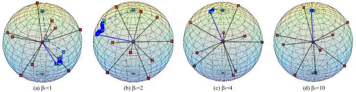
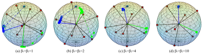
From both Fig. 5 and Fig. 6, one can observe that the neurons with larger tend to be more “fixed” (unlikely to move), and the neurons with smaller tend to move more flexibly. This can also be interpreted as the neurons with larger being more important. Such phenomena indicate that we can control the flexibility of the neurons under the learning dynamics of MHE. There is one scenario where weighted MHE may be very useful. Suppose we have known that some neurons are already well learned (e.g., some filters from a pretrained model) and we do not want these neurons to be updated dramatically, then we can use the weighted MHE and set a larger for these neurons.
Appendix E Regularizing SphereNets with MHE
SphereNets [31] are a family of network networks that learns on hyperspheres. The filters in SphereNets only focus on the hyperspherical (i.e., angular) difference. One can see that the intuition of SphereNets well matches that of MHE, so MHE can serve as a natural and effective regularization for SphereNets. Because SphereNets throw away all the magnitude information of filters, the weight decay can no longer serve as a form of regularization for SphereNets, which makes MHE a very useful regularization for SphereNets. Originally, we use the orthonormal regularization to regularize SphereNets, where is the weight matrix of a layer with each column being a vectorized filter and is an identity matrix. We compare MHE, half-space MHE and orthonormal regularization for SphereNets. In this section, all the SphereNets use the same architecture as the CNN-9 in Table 11, the training setting is also the same as CNN-9. We only evaluate SphereNets with cosine SphereConv. Note that, is actually the logarithmic hyperspherical energy (a relaxation of the original hyperspherical energy). From Table 13, we observe that SphereNets with MHE can outperform both the SphereNet baseline and SphereNets with the orthonormal regularization, showing that MHE is not only effective in standard CNNs but also very suitable for SphereNets.
| Method | CIFAR-10 | CIFAR-100 | ||||
| MHE | 5.71 | 5.99 | 5.95 | 27.28 | 26.99 | 27.03 |
| Half-space MHE | 6.12 | 6.33 | 6.31 | 27.17 | 27.77 | 27.46 |
| A-MHE | 5.91 | 5.98 | 6.06 | 27.07 | 27.27 | 26.70 |
| Half-space A-MHE | 6.14 | 5.87 | 6.11 | 27.35 | 27.68 | 27.58 |
| SphereNet with Orthonormal Reg. | 6.13 | 27.95 | ||||
| SphereNet Baseline | 6.37 | 28.10 | ||||
Appendix F Improving AM-Softmax with MHE
We also perform some preliminary experiments for applying MHE to additive margin softmax loss [51] which is a recently proposed well-performing objective function for face recognition. The loss function of AM-Softmax is given as follows:
| (19) |
where is the label of the training sample , is the mini-batch size, is the hyperparameter that controls the degree of angular margin, and denotes the angle between the training sample and the classifier neuron . is the hyperparameter that controls the projection radius of feature normalization [52, 51]. Similar to our SphereFace+, we combine full-space MHE to the output layer to improve the inter-class feature separability. It is essentially following the same intuition of SphereFace+ by adding an additional loss function to AM-Softmax loss.
Experiments. We perform a preliminary experiment to study the benefits of MHE for improving AM-Softmax loss. We use the SphereFace-20 network and trained on CASIA-WebFace dataset (training settings are exactly the same as SphereFace+ in the main paper and [29]). The hyperparameters for AM-Softmax loss exactly follow the best setting in [51]. AM-Softmax achieves 99.26% accuracy on LFW, while combining MHE with AM-Softmax yields 99.37% accuracy on LFW. Such performance gain is actually very significant in face verification, which further validates the superiority of MHE.
Appendix G Improving GANs with MHE
We propose to improve the discriminator of GANs using MHE. It has been pointed out in [35] that the function space from which the discriminators are learned largely affects the performance of GANs. Therefore, it is of great importance to learn a good discriminator for GANs. As a recently proposed regularization to stabilize the training of GANs, spectral normalization (SN) [35] encourages the Lipschitz constant of each layer’s weight matrix to be one. Since MHE exhibits significant performance gain for CNNs as a regularization, we expect MHE can also improve the training of GANs by regularizing its discriminator. As a result, we perform a preliminary evaluation on applying MHE to GANs.
Specifically, for all methods except WGAN-GP [9], we use the standard objective function for the adversarial loss:
| (20) |
where is a latent variable, is the normal distribution , and is a deterministic generator function. We set to 128 in all the experiments. For the updates of , we used the alternate cost proposed by [7] as used in [7, 54]. For the updates of , we used the original cost function defined in Eq. (20).
Recall from [35] that spectral normalization normalizes the spectral norm of the weight matrix such that it makes the Lipschitz constraint to be one:
| (21) |
We apply MHE to the discriminator of standard GANs (with the original loss function in [7]) for image generation on CIFAR-10. In general, our experimental settings and training strategies (including architectures in Table 15) exactly follow spectral normalization [35]. For MHE, we use the half-space variant with Euclidean distance (Eq. (1)). We first experiment regularizing the discriminator using MHE alone, and it yields comparable performance to SN and orthonormal regularization. Moreover, we also regularize the discriminator simultaneously using both MHE and SN, and it can give much better results than using either SN or MHE alone. The results in Table 14 show that MHE is potentially very useful for training GANs.
| Method | Inception score |
| Real data | 11.24.12 |
| Weight clipping | 6.41.11 |
| GAN-gradient penalty (GP) | 6.93.08 |
| WGAN-GP [9] | 6.68.06 |
| Batch Normalization [21] | 6.27.10 |
| Layer Normalization [2] | 7.19.12 |
| Weight Normalization [40] | 6.84.07 |
| Orthonormal [4] | 7.40.12 |
| SN-GANs [35] | 7.42.08 |
| MHE (ours) | 7.32.10 |
| MHE + SN [35] (ours) | 7.59.08 |
G.1 Network Architecture for GAN
We give the detailed network architectures in Table 15 that are used in our experiments for the generator and the discriminator.
| dense 512 |
| 44, stride=2 deconv. BN 256 ReLU |
| 44, stride=2 deconv. BN 128 ReLU |
| 44, stride=2 deconv. BN 64 ReLU |
| 33, stride=1 conv. 3 Tanh |
| RGB image |
| 33, stride=1 conv 64 lReLU |
| 44, stride=2 conv 64 lReLU |
| 33, stride=1 conv 128 lReLU |
| 44, stride=2 conv 128 lReLU |
| 33, stride=1 conv 256 lReLU |
| 44, stride=2 conv 256 lReLU |
| 33, stride=1 conv. 512 lReLU |
| dense 1 |
G.2 Comparison of Random Generated Images
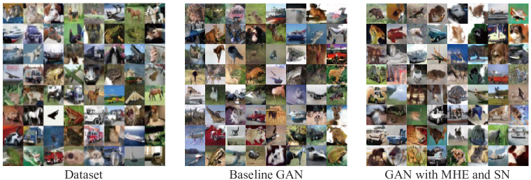
We provide some randomly generated images for comparison between baseline GAN and GAN regularized by both MHE and SN. The generated images are shown in Fig. 7.
Appendix H More Results on Class-imbalance Learning
H.1 Class-imbalance learning on CIFAR-100
We perform additional experiments on CIFAR-100 to further validate the effectiveness of MHE in class-imbalance learning. In the CNN used in the experiment, we only apply MHE (i.e., full-space MHE) to the output layer, and use MHE or half-space MHE in the hidden layers. In general, the experimental settings are the same as the main paper. We still use CNN-9 (which is a 9-layer CNN from Table 11) in the experiment. Slightly differently from CIFAR-10 in the main paper, the two data imbalance settings on CIFAR-100 include 1) 10-class imbalance (denoted as Single in Table 16) - All classes have the same number of images but 10 classes (index from 0 to 9) have significantly less number (only 10% training samples compared to the other normal classes), and 2) multiple class imbalance (denoted by Multiple in Table 16) - The number of images decreases as the class index decreases from 99 to 0. For the multiple class imbalance setting, we set the number of each class equals to . Experiment details are similar to the CIFAR-10 experiment, which is specified in Appendix A. The results in Table 16 show that MHE consistently improves CNNs in class-imbalance learning on CIFAR-100. In most cases, half-space MHE performs better than full-space MHE.
| Method | Single | Multiple |
| Baseline | 31.43 | 38.39 |
| Orthonormal | 30.75 | 37.89 |
| MHE | 29.30 | 37.07 |
| Half-space MHE | 29.40 | 36.52 |
| A-MHE | 30.16 | 37.54 |
| Half-space A-MHE | 29.60 | 37.07 |
H.2 2D CNN Feature Visualization
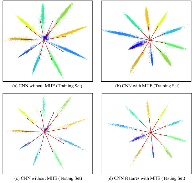
The experimental settings are the same as the main paper. We supplement the 2D feature visualization on testing set in Fig. 8. The visualized features on both training set and testing set well demonstrate the superiority of MHE in class-imbalance learning. In the CNN without MHE, the classifier neuron of the imbalanced training data is highly biased towards another class, and therefore can not be properly learned. In contrast, the CNN with MHE can learn uniformly distributed classifier neurons, which greatly improves the network’s generalization ability.
Appendix I More results of SphereFace+ on Megaface Challenge
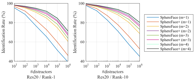
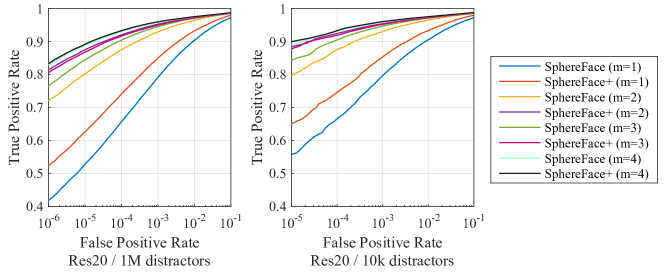
We give more experimental results of SphereFace+ on Megaface challenge. The results in Table 17 evaluate SphereFace+ under different and show that SphereFace+ consistently outperforms the SphereFace baseline. It indicates that MHE also enhances the verification rate on Megaface challenge. Our results of Identification Rate vs. Distractors Size and ROC curve are showed in Fig. 9 and Fig. 10, respectively.
| SphereFace | SphereFace+ | |
| 1 | 42.46 | 52.02 |
| 2 | 71.79 | 80.94 |
| 3 | 76.34 | 80.58 |
| 4 | 82.56 | 83.39 |
Appendix J Training SphereFace+ on MS-Celeb and IMDb-Face datasets
All the previous results of SphereFace+ are trained on the relatively small-scale CASIA-WebFace dataset which only has 0.49M images. In order to comprehensively evaluate SphereFace+, we further train the SphereFace+ model on two much larger datasets: MS-Celeb [10] (8.6M images) and IMDb-Face [50] (1.7M images). Specifically, we use the SphereFace-20 network architecture [29] for both SphereFace and SphereFace+ We evaluate SphereFace+ on both LFW (verification accuracy) and MegaFace (rank-1 identification accuracy with 1M distractors), and the results are given in Table 18. From Table 18, we can observe that SphereFace+ still consistently outperforms SphereFace with a noticeable margin. Note that, our SphereFace performance may differ from the ones in [50], because we use different face detection and alignment tools. Most importantly, the results in Table 18 are fairly compared, since all the preprocessings and network architectures used here are the same.
| Dataset | # images | # identities | Method | LFW (%) | MegaFace (%) |
| IMDb-Face | 1.7M | 56K | SphereFace | 99.53 | 72.89 |
| SphereFace+ | 99.57 | 73.15 | |||
| MS-Celeb | 8.6M | 96K | SphereFace | 99.48 | 73.93 |
| SphereFace+ | 99.5 | 74.16 | |||
| CASIA-WebFace | 0.49M | 10.5K | SphereFace | 99.27 | 70.68 |
| SphereFace+ | 99.32 | 71.30 |