The classical D-type expansion of spherical H ii regions

Abstract

Recent numerical and analytic work has highlighted some shortcomings in our understanding of the dynamics of H ii region expansion, especially at late times, when the H ii region approaches pressure equilibrium with the ambient medium. Here we reconsider the idealized case of a constant radiation source in a uniform and spherically symmetric ambient medium, with an isothermal equation of state. A thick-shell solution is developed which captures the stalling of the ionization front and the decay of the leading shock to a weak compression wave as it escapes to large radii. An acoustic approximation is introduced to capture the late-time damped oscillations of the H ii region about the stagnation radius. Putting these together, a matched asymptotic equation is derived for the radius of the ionization front which accounts for both the inertia of the expanding shell and the finite temperature of the ambient medium. The solution to this equation is shown to agree very well with the numerical solution at all times, and is superior to all previously published solutions. The matched asymptotic solution can also accurately model the variation of H ii region radius for a time-varying radiation source.

1 Introduction

Massive stars are an important source of mass and energy to the interstellar medium (ISM), through the radiation they emit, the strong winds which they drive, and the supernova explosions by which they end their lives. Feedback from massive star formation can redistribute matter, sculpting the ISM and potentially inhibiting or promoting star formation (Walch et al., 2015; Dale, 2015). Supernovae are the dominant feedback agent driving turbulent gas flows in star-forming regions (Mac Low & Klessen, 2004). For a given star-formation episode, however, ionizing radiation starts to be emitted as soon as the first massive star reaches the zero-age main sequence. Heating by this ionizing radiation is the dominant feedback process before supernovae commence for all but the most massive, compact star clusters where the escape velocity is above $20{\rm\,km\,s^{-1}}$ (Henney, 2007; Dale et al., 2014; Ngoumou et al., 2015).

The simplest model of the effect of photoionization on the ISM, a spherically symmetric expansion of a bubble of ionized gas around point source of ultraviolet photons with constant flux, is a classical problem in ISM physics (Spitzer, 1978; Dyson & Williams, 1997; Osterbrock & Ferland, 2006). This system develops through a number of stages. At first, each photon emitted leads to an additional ionization, so the speed of expansion of the ionization region is determined by the ionizing luminosity. Soon, the ionized material starts to recombine, and an increasing fraction of the luminosity is taken up in maintaining the level of ionization. The expansion of the front slows as a result both of geometric dilution of the ionizing radiation and the increasing rate of recombinations in the ionized region. Within the ionized region, the pressure increases due to both the larger number of free particles and the higher material temperature. As a result, when the rate of expansion of the ionization front slows to approximately twice the sound speed within the ionized region, a strong shock is generated at its surface which moves ahead of the ionization front into the surrounding neutral material. As time progresses, this shock weakens and its separation from the ionization front increases. The ionization front slows and eventually relaxes to an equilibrium radius at which the pressure in the rarefied ionized region balances that in the unshocked external medium.

While clearly an idealization of the expansion of an H ii region around a young massive star, this model captures many essential features of its dynamics. The analytic formulation of this problem follows classic work on ionization fronts (Kahn, 1954) by taking the ionized gas to be isothermal with a temperature $T\approx 10^{4}$ K and the neutral gas also isothermal, but with a far lower temperature ($T\approx 10\mbox{--}100{\rm\,K}$).

Early analytic and numerical studies of a spherically symmetric H ii region are summarised by Mathews & O’Dell (1969), by which time ground-breaking numerical simulations had been performed (Lasker, 1966) but an analytic form for the expansion as a function of time had not been obtained. An analytic solution for the spherical expansion of an H ii region was presented by Spitzer (1978) by assuming the equality of total pressure on either side of the swept-up shell, and this became the standard solution (e.g. Dyson & Williams, 1997). It was, however, missing an essential concept: the inertia of the swept-up shell (Hosokawa & Inutsuka, 2006), as had already been treated by Elmegreen & Lada (1977), albeit for a planar rather than spherical front. Simulations by Raga et al. (2012b) found that the ionization front overshoots the equilibrium radius at late times and relaxes back, a behaviour which the Spitzer and Hosokawa & Inutsuka solutions do not capture.

Bisbas et al. (2015) compared results for this problem for multiple time-dependent flow dynamics codes, finding good agreement between them. This paper also compared these computational results with a number of analytical and semi-analytical models for the expansion of the H ii region. At early time, where the shocked shell is thin, much better agreement was found with the model of Hosokawa & Inutsuka (2006) than that of Spitzer (1978). Although Raga’s modification of the Spitzer solution Raga et al. (2012a), referred to below as Raga-II, relaxes to the correct radius of the H ii region as $t\rightarrow\infty$, none of the available models provides a good description of the later time development of the H ii region as it comes into pressure equilibrium with its environment. The intention of the present paper is to remedy this.

While the late time relaxation of an H ii region is more subject to details such as the changing ultraviolet radiance of the central star and the density distribution of the interstellar medium environment, the idealized problem which we consider is not without practical relevance. H ii regions form an important component of the interstellar medium in the disks of late type galaxies. The shells which they drive are a source for the turbulent motions within this medium (e.g. Gritschneder et al., 2009; Medina et al., 2014; Arthur et al., 2016). The nature of their response to variations in the pressure of the interstellar medium will also have important effects, for example, on the nature of the response of the medium to supernova explosions (e.g. Rogers & Pittard, 2013) and density waves in galactic disks. It is also very useful to have reference solutions which capture the full evolution of an H ii region for the purposes of validating computer algorithms.

In this paper, we first discuss the dimensionless parameters which characterize the problem. We then present our reference numerical calculation, before developing a range of analytic and semi-analytic treatments for the structure of the evolving H ii region, which we compare to the numerical solution. The most detailed of these is compared to additional numerical calculation where the ionization source is changed during the evolution. Finally, we summarize our results, including the potential for their application as a sub-grid model in larger scale simulations of the interstellar medium.

2 Controlling parameters

To define how wide a parameter space must be covered by an analytic treatment for the problem of expansion of an H ii region, it is helpful to determine the dimensionless parameters which control the process, as this will determine whether cases can be scaled to a single common solution.

We consider the dimensional controlling parameters for the expansion of a dust-free H ii region in an isothermal environment free of magnetic fields. These are the particle density of the environment, $n_{0}$, the source rate of ionizing photons $Q_{0}$, and the hot and cold material sound speeds, $c_{\mathrm{i}}$ and $c_{0}$. We use the sound speeds and particle density to capture the dependency of the system on molecular mass. The relevant atomic physics is captured by the ionization cross-section $a$ and the case B recombination coefficient $\alpha_{\rm B}$, into excited states only. Applying case B implies that the H ii region is assumed to be very optically thick to Lyman continuum photons, and hence that the photons emitted by direct recombinations to the $n=1$ level will ionize some neighbouring atom, leading to no net recombination (known as the ‘on-the-spot’ approximation, Osterbrock & Ferland, 2006). Williams & Henney (2009) explicitly treat the radiation transfer of the diffuse Lyman continuum, and confirm that this will typically have a negligible effect on the structure of the H ii region compared to the case B approximation.

With six parameters, we are looking for four dimensionless parameters for the problem. The forms we will consider for these parameters are

$${c_{\mathrm{i}}\over c_{0}};\quad{Q_{0}\over n\alpha_{\rm B}};\quad U\sim{n^{1/3}Q_{0}^{1/3}\alpha_{\rm B}^{2/3}\over c_{\mathrm{i}}};\quad{ac_{\mathrm{i}}\over\alpha_{\rm B}}.$$ (1)

The first two of these parameters have obvious interpretations: the ratio of sound speeds determines the initial over-pressure (and eventual under-density) of the H ii region, and the second parameter is the total number of particles in the initial nebula.

The third parameter $U$ is proportional to the ratio of the ionizing photon flux to the thermal particle flux at the initial (Strömgren, 1939) radius, $R_{\rm St}$, if absorption were neglected. $R_{\rm St}$ satisfies

$$Q_{0}={4\pi\over 3}\alpha_{\rm B}n^{2}R_{\rm St}^{3}\;.$$ (2)

Equivalently, $U$ is the ratio of the sound-crossing time of the nebula to the characteristic time for ions to recombine. It may also be related to the column density through the ionized nebula, $N$, by

$$U\sim{\alpha_{\rm B}N\over c_{\mathrm{i}}}.$$ (3)

This is a typical ionization parameter.

The fourth parameter is dependent only on atomic physics, so will not vary substantially between observed nebulae. The product of the third and fourth parameters is independent of $c_{\mathrm{i}}$, and determines the ratio of the Strömgren radius to the ionization front thickness, $\sim naR_{\rm St}$ as well as the mean level of ionization within the nebula, since locally

$${x^{2}\over 1-x}={aJ_{\rm i}\over n\alpha_{\rm B}},$$ (4)

and $\left\langle J_{\rm i}\right\rangle\sim Q_{0}/4\pi R_{\rm St}^{2}$: ionization fronts are geometrically thin for the same reason that their cores are almost fully ionized, and what matters most for dynamical studies is that both these statements are true.

Typical values of $Q_{0}\simeq 10^{49}{\rm\,s^{-1}}$, $\alpha_{\rm B}\simeq 2\times 10^{-13}{\rm\,cm^{3}\,s^{-1}}$, $a\simeq 6\times 10^{-18}{\rm\,cm^{-2}}$, $c_{\mathrm{i}}=10{\rm\,km\,s^{-1}}$, $c_{0}=0.3{\rm\,km\,s^{-1}}$ give

$${c_{\mathrm{i}}\over c_{0}} \simeq 30,$$ (5)

$${Q_{0}\over n\alpha_{\rm B}} \simeq {5\times 10^{61}\over n},$$ (6)

$${n^{1/3}Q_{0}^{1/3}\alpha_{\rm B}^{2/3}\over c_{\mathrm{i}}} \simeq 74n^{1/3},$$ (7)

$${ac_{\mathrm{i}}\over\alpha_{\rm B}} \simeq 30.$$ (8)

The second parameter is so overwhelmingly large that the behaviour of nebulae will almost always be in the asymptotic regime which means that the structure of the nebula can be well modelled as a continuum fluid. The first and fourth parameters are weakly dependent on the circumstances of a particular nebula, but have a similar scale to the third parameter. Hence the structure and evolution of H ii regions is only to be significantly affected by the value of the third dimensionless parameter.

The structure may pass through a number of regimes through the lifetime of an individual nebula, as the value of this parameter varies with respect to that of the first and fourth parameters. However, these effects will generally be quite weak, so long as the mean ionization within the region remains close to complete (and if the radiation pressure due to the ionizing continuum is ignored). Varying the ionization parameter will affect the spectrum of emission line radiation more significantly than it does the gross hydrodynamics of the expansion of the H ii region.

3 Numerical calculation

We will use the Early Phase test of the StarBench project presented in Bisbas et al. (2015) to compare with a number of analytical approximations that will be discussed in detail in Section 4. We have run the calculation beyond the latest time considered in the previous paper, to allow the asymptotic behaviour to be studied. A larger domain has to be considered to ensure that the out-going expansion wave remains on the mesh.

For reference, in this problem the density of the neutral medium (consisting of pure hydrogen) is taken to be $\rho_{\rm o}=5.21\times 10^{-21}\,{\rm g}\,{\rm cm}^{-3}$. We consider a source emitting ionizing photons at a constant rate of $Q_{0}=10^{49}\,{\rm s}^{-1}$. The resulting two-phase media have temperatures $T_{\rm i}=10^{4}\,{\rm K}$ and $T_{0}=10^{2}\,{\rm K}$ for the ionized ($\mu=0.5$) and neutral ($\mu=1$) regimes respectively corresponding to sound speeds of $c_{\mathrm{i}}=12.85\,{\rm km/s}$ and $c_{0}=0.91\,{\rm km/s}$. The initial Strömgren radius is $R_{\rm St}=0.314\,{\rm pc}$ and we evolve for $t=200\,{\rm Myr}$, which allows for several oscillations of the Hii region about the stagnation radius of $R_{\rm Stag}=(c_{\mathrm{i}}/c_{0})^{4/3}R_{\rm St}=10.75\,{\rm pc}$ (Raga et al., 2012a).

We use the results of numerical calculations performed by the Glide code. Glide is a spherically-symmetric Lagrangian code which participated in the StarBench project, and is described in Bisbas et al. (2015). While this code has not been widely applied, its results agree well with other codes in the StarBench comparison, and its algorithm minimizes the effects of numerical mixing on the evolution of the H ii region compared to solving on a mesh fixed in space.

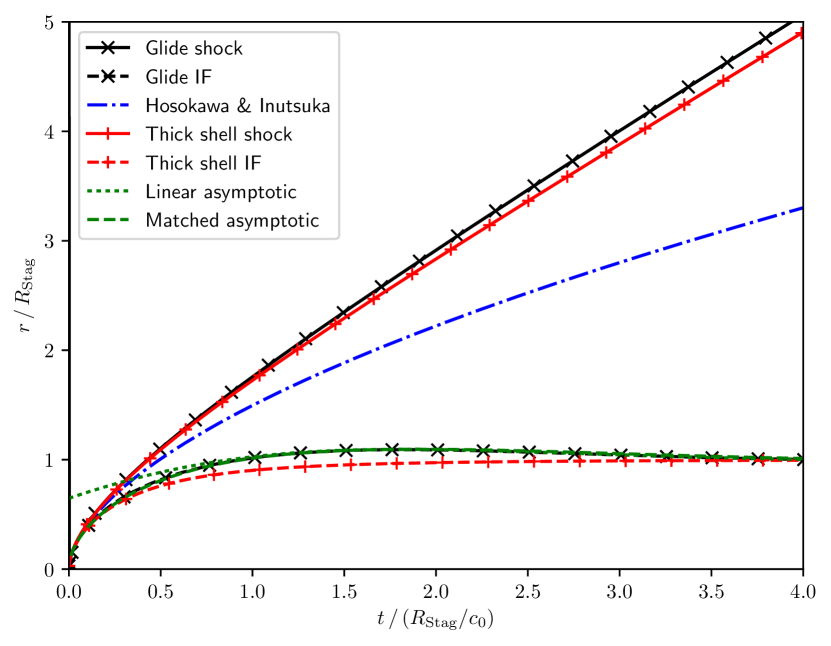
Figure 1: Ionization and shock front positions from a fluid dynamical calculation with Glide, compared to several approximations. The vertical axis is the radial distance as a fraction of $R_{\rm Stag}$, the horizontal axis the time as a function of the neutral-phase sound crossing time $R_{\rm Stag}/c_{0}$.

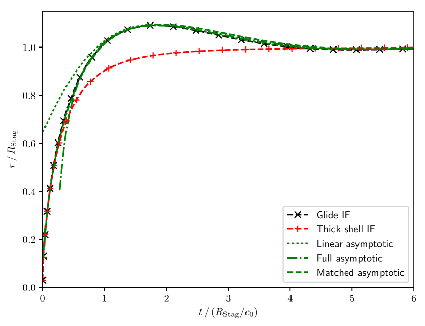
Figure 2: As Figure 1, but scaled to emphasize early- to mid-time expansion of the ionization front.

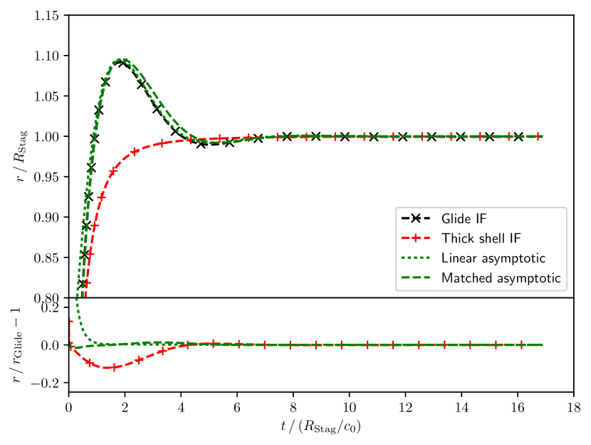
Figure 3: As Figure 1, but scaled to emphasize late-time relaxation. The lower panel shows the fractional residual between each of the approximations and the simulation result.

To capture the different phases of evolution of this system, we show three separate plots, Figures 1, 2 and 3, which, respectively, capture the thickening of the shocked shell, ionization front overshoot and late time relaxation of the ionized bubble. These plots also show a number of analytical and semi-analytical models for the position of the ionization and shock fronts, which we will discuss in the following section. Figure 1 shows how the leading shock and ionization front initially move together. As the ionization front approaches the equilibrium expansion radius, both fronts slow, and the shell between them becomes geometrically thick. The speed of the shock front reduces asymptotically to the sound speed in the neutral medium. Figure 2 shows that the ionization front does expand beyond its equilibrium radius by a small amount, as a result of the inertia of the material within the shell, but subsequently relaxes back towards its equilibrium radius. Figure 3 shows that this relaxation is in fact a strongly damped oscillation.

4 Analytic models

The development of an H ii region passes through a number of regimes with time, as different flow parameters become dominant. In this paper, we concentrate on the expansion of the region once the ionization front has reached the weak D-type phase, where the shocked neutral material ahead of the front is close to pressure equilibrium with the ionized material around the central star. We will extend well-known solutions in two asymptotic limits, the initial thin expanding shell and the late-time pressure equilibrium between the ionized gas and its environment, towards an intermediate bridging regime. At early time, this requires the extension of the analysis by Hosokawa & Inutsuka (2006) to allow for the thickening of the shocked shell as its expansion slows towards the sound speed in the neutral environment; at late time, we generalize the model of oscillations of an explosively-driven bubble by Keller & Kolodner (1956) to the boundary conditions appropriate for a photoionized bubble. A similar approach was applied by Shabala & Alexander (2009) to sound wave oscillations in galaxy clusters.

4.1 Thin shell equations

The early time behaviour of the H ii region was studied in detail by Bisbas et al. (2015) using a wide range of numerical hydrodynamic codes. That work confirmed that the solution at early times was well described by the analytic solution of Hosokawa & Inutsuka (2006).

The motion of the shell is treated using rate of change of the total momentum of the swept-up shell (Elmegreen & Lada, 1977; Hosokawa & Inutsuka, 2006). Assuming that the shell is thin, this gives

$$\frac{d}{dt}(M\dot{R})=4\pi R^{2}(P_{1}-P_{0})\;,$$ (9)

which also includes the correction for the effect of the pressure in the external medium introduced by Raga et al. (2012b), and in which

$$M =\frac{4\pi}{3}\rho_{0}R^{3}$$ (10)

$$P_{1} =\rho_{1}c_{\mathrm{i}}^{2}$$ (11)

$$P_{0} =\rho_{0}c_{0}^{2}$$ (12)

$$\rho_{1} =\rho_{0}\left(\frac{R_{\rm St}}{R}\right)^{3/2}$$ (13)

are the equation of mass conservation, the isothermal equations of state assumed in the ionized and neutral material, and the condition for the ionization equilibrium. The initial (constant) background medium has density $\rho_{0}$ and pressure $P_{0}$; and the isothermal sound speeds in neutral ($c_{0}$) and ionized ($c_{\mathrm{i}}$) gas are constant parameters of the model, as is the initial Strömgren radius of the photoionized region.

Substituting in, we find an equation equivalent to the system derived by Raga et al. (2012a), and referred to as ‘Raga-II’ by Bisbas et al. (2015),

$${d\over dt}\left(R^{3}\dot{R}\right)=3R^{2}\left[c_{\mathrm{i}}^{2}\left(R_{\rm St}\over R\right)^{3/2}-c_{0}^{2}\right].$$ (14)

This equation has been constructed so that a static bubble at the stagnation radius is an equilibrium solution. However, it is symmetric in time, so its solutions must also be symmetric, either repeating with a finite period or extending to $t\to\pm\infty$. This explains the periodic oscillating behaviour of the solutions in the limit of rapid recombination found by Raga et al. (2012a).

Multiplying equation (14) by $R^{3}\dot{R}$, it can be integrated to give

$${1\over 2}\left(R^{3}\dot{R}\right)^{2}=\left[{2\over 3}c_{\mathrm{i}}^{2}R_{\rm St}^{3/2}R^{9/2}-{1\over 2}c_{0}^{2}R^{6}\right]+{\rm const}.$$ (15)

If we assume that both $c_{0}$ and the integration constant are zero, then the equation can be integrated again to give the Hosokawa & Inutsuka (2006) solution

$$R=R_{\rm St}\left(1+{7\over 4}\sqrt{4\over 3}{c_{\mathrm{i}}t\over R_{\rm St}}\right)^{4/7},$$ (16)

where we have taken $R=R_{\rm St}$ at $t=0$ to define the constant of integration (which is simply a time offset of the solution).

Ignoring the term in $c_{0}$ is reasonable so long as $\dot{R}\gg c_{0}$. The assumption that the constant of integration in equation (15) can be taken as zero is more arbitrary, being a requirement in order for the system to have a simple closed form solution, rather than being determined from the initial conditions of the system. Equation (16) gives an initial velocity of $2c_{\mathrm{i}}/\sqrt{3}$ at $R=R_{\rm St}$; equation (15) can be integrated numerically for differing values of this initial velocity, but the results tend to converge with time.

In Figure 1, this approximation is compared to our numerical integral. At early time, the expansion rate agrees well (as already demonstrated by Raga et al., 2012a; Bisbas et al., 2015). At later time, however, the shock wave moves away more rapidly than equation (16), while the expansion of the ionization front stalls. Clearly, a more detailed model for the structure of the H ii region is required to derive a more accurate analytic approximations for the expansion of shock and ionization fronts.

4.2 Thick shell approximation

Equation (16) does not differentiate between the radius of the ionization front and that of the shock front, i.e. it assumes that the swept-up shell of material between them is thin. This is a reasonable assumption when the outgoing shock speed is far greater than the sound speed in the neutral material, as the isothermal equation of state means that the shocked material compresses by a factor the square of the shock Mach number. However, as the H ii region develops, the region of swept-up neutral material thickens and these fronts move apart. To improve the accuracy of the formulation at later times, this distinction must be taken into account.

We consider the expansion of the swept-up shell as it becomes geometrically thick. Assuming that the material within it has approximately constant velocity, the rate of change of its radial momentum can be modelled by generalizing equation (14) to become

$${d\over dt}\left(M(R_{\rm SF})\dot{R}_{\rm shell}\right)=4\pi R_{\rm SF}^{2}\rho_{0}\left[c_{\mathrm{i}}^{2}\left(R_{\rm St}\over R_{\rm IF}\right)^{3/2}-c_{0}^{2}\right].$$ (17)

where the terms in $R$ in equation (14) have been modified to distinguish $R_{\rm SF}$ as the radius of the shock, $R_{\rm IF}$ as the radius of the ionization front, and $\dot{R}_{\rm shell}$ as the velocity of material in the shocked shell. From the isothermal jump conditions, we take

$$\dot{R}_{\rm shell}=\dot{R}_{\rm SF}-{c_{0}^{2}\over\dot{R}_{\rm SF}},$$ (18)

which can be substituted in equation (17) to derive an second-order equation for $\dot{R}_{\rm SF}$. This relation between the shock velocity and shell expansion rate was also used by Raga et al. (2012b).

Equation (17) assumes approximate pressure balance through the shell. The outward force on the shell includes both the force at the ionization front $4\pi R_{\rm IF}^{2}P_{1}$ and the hydraulic amplification through the shell, i.e. it is

$$F\simeq 4\pi R_{\rm IF}^{2}P_{1}+\int_{R_{\rm IF}}^{R_{\rm SF}}\left[2P(r)\over r\right]4\pi r^{2}{\rm d}r\simeq 4\pi R_{\rm SF}^{2}P_{1}.$$ (19)

The shell thickness can be derived from mass conservation and approximate pressure balance at the ionization front, assuming that the shell has constant density, so

$$R_{\rm IF}^{3/2}={2c_{\mathrm{i}}^{2}R_{\rm St}^{3/2}\over c_{0}^{2}+\sqrt{c_{0}^{4}+4c_{\mathrm{i}}^{2}\left(c_{\mathrm{i}}^{2}-c_{0}^{2}\right)\left(R_{\rm St}/R_{\rm SF}\right)^{3}}}.$$ (20)

If $R_{\rm SF}=R_{\rm St}$, or $c_{0}/c_{\mathrm{i}}\to 0$, $R_{\rm IF}=R_{\rm SF}$ as expected. If $R_{\rm SF}\to\infty$, $R_{\rm IF}\to(c_{\mathrm{i}}/c_{0})^{4/3}R_{\rm St}$, which is also the late-time equilibrium solution. This equation for the ionization front radius in terms of the shock front radius allows the equation for the shock front position to be integrated.

From Figures 1 and 2, we see that the thick shell equations capture the overall behaviour of the ionization front and shock front quite well, in particular the eventual expansion of the shock front at the sound speed in the neutral medium, and the final equilibrium radius of the ionization front. However, in the numerical calculations, the inertia of the shell leads the ionization front to overshoot, an effect which cannot be captured as a result of the simplified model of the structure of the swept-up shell. We will now develop a more detailed model to capture the overshoot and relaxation of the ionization front radius.

4.3 Late time behaviour of the H ii region

At late time, the leading shock expands to a distance $R_{\rm SF}\gg R_{\rm Stag}=(c_{\mathrm{i}}/c_{0})^{4/3}R_{\rm St}$, so the behaviour of the H ii region may be treated independently of the leading shock. The resulting system is similar to the oscillation of a spherical bubble in a dense fluid, which was studied by Keller & Kolodner (1956). However, the boundary conditions at the inner edge of the dense fluid are determined by jump conditions at a weak D-type ionization front, rather than by a material discontinuity. In this section, we generalize Keller & Kolodner’s approach to the late time behaviour of an H ii region.

The equations governing the motion outside the ionization front are as given by Keller & Kolodner, but here we adapt them to the case of isothermal flow. The Euler equations for isothermal flow are

$$\dot{\rho}+\nabla\cdot\left(\rho{\mathbf{v}}\right) =0$$ (21)

$$\rho\dot{\mathbf{v}}+\rho{\mathbf{v}}\cdot\nabla{\mathbf{v}} =-\nabla p=-c_{0}^{2}\nabla\rho,$$ (22)

which in the limit $v\ll c_{0}$ are solved by a velocity derived from a velocity potential $\phi$ defined by

$${\mathbf{v}}=\nabla\phi$$ (23)

which satisfies the isothermal acoustic wave equation

$$\nabla^{2}\phi={1\over c_{0}^{2}}{\partial^{2}\phi\over\partial t^{2}}.$$ (24)

Assuming purely radial flow, as a result of the symmetry of the problem, we take $\phi=\phi(r,t)$, where the radial velocity is given by $v=\partial\phi/\partial r$. Then the momentum equation becomes

$${\partial\over\partial t}\left(\phi^{\prime}\right)+{1\over 2}{\partial\over\partial r}\left(\phi^{\prime}\right)^{2}=-c_{0}^{2}{\partial\over\partial r}\log\rho,$$ (25)

which may be integrated to give

$$\dot{\phi}+{1\over 2}\left(\phi^{\prime}\right)^{2}=-c_{0}^{2}\log\rho+g(t),$$ (26)

where $g(t)$ is an arbitrary function of $t$ alone. Since as $\phi\to{\rm const}$, $\rho\to\rho_{0}$, the density of the external medium, we have $g=c_{0}^{2}\log\rho_{0}$. Hence the density can be determined from $\phi$ using the isothermal Bernoulli equation

$$-\log\left(\rho\over\rho_{0}\right)={1\over c_{0}^{2}}\left(\dot{\phi}+{1\over 2}(\phi^{\prime})^{2}\right).$$ (27)

The solution to equation (24) satisfying the boundary conditions of the problem is a general outgoing wave

$$\phi={1\over r}f\left(t-r/c_{0}\right).$$ (28)

Here $f$ is an arbitrary function which is determined by the matching conditions at the ionization front jump conditions for mass and momentum flux

$$-\rho_{i}\dot{r}_{i} =\rho\left(v-\dot{r}_{i}\right)$$ (29)

$$\rho_{i}\left[\dot{r}_{i}^{2}+c_{\mathrm{i}}^{2}\right] =\rho\left[\left(v-\dot{r}_{i}\right)^{2}+c_{0}^{2}\right],$$ (30)

where we assume that the velocity of the ionized gas in the rest frame of the system as a whole can be taken as zero. When the ionization front is reducing in radius, it will become a recombination front, but the same jump conditions will apply in the D-type limit. In the limit $v\ll c_{0}$, the boundary conditions at the D-type front at the edge of the ionized region will be

$$v =\beta\dot{r}_{i}$$ (31)

$$\rho_{i}c_{\mathrm{i}}^{2} =\rho c_{0}^{2},$$ (32)

where we define

$$\beta=\left(1-{c_{0}^{2}\over c_{\mathrm{i}}^{2}}\right)\simeq 1.$$ (33)

We also assume the Strömgren condition applies with uniform density in the ionized region

$$Q_{0}={4\over 3}\pi r_{i}^{3}\alpha_{\rm B}{\rho_{i}^{2}\over\mu_{i}^{2}}+4\pi r_{i}^{2}{\rho_{i}\over\mu_{i}}\dot{r}_{i},$$ (34)

so

$${\rho\over\rho_{0}}={1\over\xi+\sqrt{1+\xi^{2}}}\left(R_{\rm Stag}\over r_{i}\right)^{3/2},$$ (35)

where

$$\xi={3\over 2}\left(r_{i}\over R_{\rm Stag}\right)^{1/2}{c_{\mathrm{i}}^{2}\over c_{0}^{2}}{\mu_{i}\over\alpha_{\rm B}}\dot{r}_{i}$$ (36)

is typically small.

Given these boundary conditions, together with the definition of the velocity potential, equation (23), the Bernoulli equation (27) and the wave-like solution, equation (28), we have

$$\beta\dot{r}_{i}+{f^{\prime}\over r_{i}c_{0}} =-{f\over r_{i}^{2}},$$ (37)

$$\beta^{2}\dot{r}_{i}^{2}+2{f^{\prime}\over r_{i}} =3c_{0}^{2}\log\left(r_{i}\over R_{\rm Stag}\right)-2c_{0}^{2}\sinh^{-1}\xi.$$ (38)

In what follows, we will ignore the higher-order term in $\xi$ for simplicity. Eliminating $f^{\prime}$ between these equations gives an equation for $f$ in terms of $r_{i}$ and $\dot{r_{i}}$

$${2c_{0}f\over r_{i}^{2}}+3c_{0}^{2}\log\left(r_{i}\over R_{\rm Stag}\right)=\left(\beta\dot{r_{i}}-2c_{0}\right)\beta\dot{r_{i}}.$$ (39)

To eliminate $f$ from this equation, we can differentiate with respect to $t$, and substitute for $f^{\prime}$ in the result using equation (38). Note that as these expressions are evaluated at the ionization front,

$$\left.\partial f\over\partial t\right|_{r_{i}}=\left(1-{\dot{r}_{i}\over c_{0}}\right)f^{\prime},$$ (40)

and that $R_{\rm Stag}$ can vary in time if $Q_{0}$ is not constant. The result is a nonlinear second order ordinary differential equation for $r_{i}$,

$${2\over 3}r_{i}\left(c_{0}-\beta\dot{r_{i}}\right)\beta\ddot{r_{i}}+c_{0}^{2}\dot{r_{i}}+c_{0}^{2}\left(c_{0}+\dot{r_{i}}\right)\log\left(r_{i}/R_{\rm Stag}\right)$$

$$={1\over 3}\beta\dot{r_{i}}^{2}\left[\beta(c_{0}+\dot{r_{i}})-4c_{0}\right]+{1\over 3}c_{0}^{2}r_{i}{\dot{Q_{0}}\over Q_{0}}.$$ (41)

When this is solved, equation (39) can be used to determine $f$, and hence the full solution for $\rho$ and $v$ between the ionization front and the leading shock.

We will first look for the linear solution to the system with a constant ionizing flux, in the limit $c_{0}\ll c_{\mathrm{i}}$, which will capture the asymptotic behaviour of the front as it relaxes to its equilibrium stagnation radius. Writing $r_{i}=R_{\rm Stag}+\delta$, using Taylor expansions for power and logarithmic terms, and ignoring terms of higher than linear order in perturbations from equilibrium, we find that the offset of the ionization front from its equilibrium position satisfies

$${2\over 3}R_{\rm Stag}^{2}\ddot{\delta}+c_{0}R_{\rm Stag}\dot{\delta}+c_{0}^{2}\delta=0,$$ (42)

and hence

$$\delta=\delta_{0}\cos(\omega t+\psi)\exp(-\lambda t),$$ (43)

with $\omega=(15/16)^{1/2}c_{0}/R_{\rm Stag}$, $\lambda=(3/4)c_{0}/R_{\rm Stag}$, and where the amplitude $\delta_{0}$ and phase $\psi$ are arbitrary constants.

As $\beta$ is close to $1$, the major effect causing the rapid damping of oscillations for an H ii region seen in Figure 3, compared to an isothermal bubble with a constant mass of hot gas (Keller & Kolodner, 1956), must be the different manner in which the pressure within the H ii region varies with radius, rather than the mass flux through its surface.

As seen in Figure 3, the linear asymptotic solution gives an excellent fit to the relaxation of the ionization front at late time found in the numerical calculation, but Figure 2 shows that it diverges at earlier times. We will now investigate what modifications can be made to the system to improve the fit to the ionization front radius at all times.

A first approach would be to include the higher order terms in equation (41) which were ignored in deriving equation (42). However, equation (41) has a singular point, where the factor multiplying the highest derivative becomes zero, when $\beta\dot{r_{i}}=c_{0}$. Continuous solutions passing through this speed are possible only at the ionization front radius

$$r_{i}=R_{\rm Stag}\exp\left(-{6-\beta\over 3(\beta+1)}\right)\simeq 0.368R_{\rm Stag}.$$ (44)

However, in numerical simulations, the outward velocity of the front is substantially larger than $c_{0}$ when it reaches this radius, suggesting that the loss of accuracy of the approximations used when deriving equation (41) is a more immediate limitation to the accuracy of the solution than the presence of the critical point.

Figure 4: As Figure 1, but showing front velocity as a function of radius.

To the order of accuracy of the derivation leading up to equation (41), we can approximate

$$1-\beta\dot{r_{i}}/c_{0}\simeq{1\over 1+\beta\dot{r_{i}}/c_{0}},$$ (45)

which removes the singularity. Figure 3 includes a comparison with the numerical solution of equation (41) with this modification to the leading term (labelled as the ‘Full asymptotic’ case). While including additional terms in the approximation makes the semi-analytic solution more accurate at intermediate times, it diverges from the results of the full dynamical simulation rapidly at earlier times. This behaviour is fairly typical when a higher order solution is based on expansions at a single time, where increasing accuracy around this point can lead to more rapidly divergent behaviour away from it. As we will see next, a better representation may be derived by considering the asymptotic behaviour of the solution both at early and late times.

As equation (41) is a second-order autonomous ordinary differential equation, it may be converted into a system of two independent first-order ODEs, one of which is formally independent of time. Taking $q=\dot{r_{i}}/c_{0}$, the second time derivative may be replaced by $\ddot{r_{i}}=c_{0}^{2}q{\rm d}q/{\rm d}r_{i}$, to become

$${2\over 3}\left(1-\beta q\right)\beta q{{\rm d}q\over{\rm d}r_{i}}+q+\left(1+q\right)\log(r_{i}/R_{\rm Stag})$$

$$={1\over 3}\beta q^{2}\left[\beta q-(4-\beta)\right].$$ (46)

Plotting $q=\dot{r_{i}}/c_{0}$ against $r_{i}$ thus allows the results of the various approximations to be compared independent of any arbitrary time offset. Figure 4 shows the velocity of the ionization front as a function of its radius, derived from the simulated data and for various approximations. The linear approximation to the late time behaviour forms a logarithmic spiral, while the full asymptotic solution diverges from the numerical results in the opposite direction.

4.4 Matched asymptotic solution

We will now look for an equation for the position of the ionization front which can capture its behaviour throughout its evolution with good accuracy, by modifying equation (41) with terms which are small at late time, but which will mean that it agrees with the thin shell system, described by equation (14), at early times.

Equation (14) can be expressed as

$$R\ddot{R}+3\dot{R}^{2}=3c_{0}^{2}\left[\left(R_{\rm Stag}\over R\right)^{3/2}-1\right],$$ (47)

and we will now look to match terms at the same order equation (41) while we can still assume $R\simeq r_{i}$. Adding lower-order terms to equation (47) so that it matches the behaviour of the solution at late time, term-by-term in Taylor expansions, in particular requiring that the linear-order terms which control the late-time behaviour in Equation (41) are exact, gives

$$\beta r_{i}\ddot{r}_{i} +{1\over 2}\beta(7-\beta)\dot{r}_{i}^{2}+{3\over 2}{\dot{r}_{i}c_{0}\over 1+C\dot{r}_{i}^{2}/c_{0}^{2}}+$$

$$={c_{0}+3B\dot{r}_{i}\over c_{0}+B\dot{r}_{i}}c_{0}^{2}\left[\left(R_{\rm Stag}\over r_{i}\right)^{3/2}-1\right]+{1\over 2}c_{0}r_{i}{\dot{Q}_{0}\over Q_{0}},$$ (48)

where $B=(1+\beta)/2$ and $C=2.25$, and we have included the source term required if the luminosity of the source varies. This modified form accounts for both the effects of the finite temperature of the neutral material, and the late time relaxation to equilibrium. The constant $B$ is determined by the matching procedure, but the reduction of the damping term linear in $\dot{r}_{i}$ controlled by the dimensionless parameter $C$ is not. This reduction in the linear damping term is found to be necessary to obtain a good fit to the full numerical evolution, even though the quadratic term is larger at early time, when the expansion velocity of the ionization front $\dot{r}_{i}>c_{0}$.

As can be seen in Figure 3, the solution of this matched asymptotic system for the ionization front position, equation (48) fits the data from the numerical solution with good accuracy throughout. A small phase-shift is apparent in the behaviour at late time compared to the linear solution, as the phase is no longer a free parameter which can be varied to optimize the agreement. Figure 4 shows excellent agreement, showing that this phase-shift corresponds to a small time offset in the late-time behaviour.

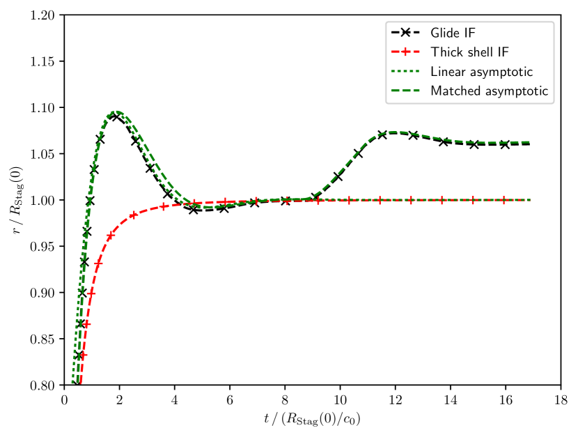
Figure 5: As Figure 1, but scaled to emphasize late-time relaxation, with ionizing luminosity linearly increasing to 120 per cent of its initial value between $100$ and $125{\rm\,Myr}$ (i.e. $tc_{0}/R_{\rm Stag}(0)=8.6$ and $10.8$). Note that the time and radius are scaled to the initial stagnation radius, $R_{\rm Stag}(0)$. The change in luminosity is not implemented in the linear asymptotic form or thick shell forms, which are included simply for cross-reference.

Equation (48) is general enough to allow for the variation of the ionizing luminosity of the source with time, by varying $R_{\rm Stag}$ to reflect the changing value of $Q_{0}$. In Figure 5, we compare the results of equation (48) with the variation of ionization front radius when the ionizing luminosity is assumed to increase linearly to $1.2\times 10^{49}$ from $100{\rm\,Myr}=8.64R_{\rm Stag}/c_{0}$ to $125{\rm\,Myr}$. The agreement between the model and the numerical solution as the ionizing flux varies is excellent, as expected so long as the relative rate of change of ionizing flux is slow compared to the sound crossing time of the ionized bubble.

5 Discussion and conclusions

In this paper, we have extended the analytic study of the expansion of an H ii region in the idealized case of a constant source and uniform ambient medium. The agreement between model and simulation during the D-type expansion phase has been improved compared to previous works, to within 2 per cent relative error at all times. A thick-shell approximation allows for the stalling of the ionization front and decay of the leading shock to a weak compression wave as it escapes to large radii. An acoustic approximation, modifying the work of Keller & Kolodner (1956) to take account of the different boundary conditions at the ionization front, captures the late-time oscillations of the H ii region about the stagnation radius, and its response to variations in ionizing luminosity.

We have examined the dynamics of H ii regions in significantly greater depth than previous work; the thick-shell solution and the asymptotic solutions give considerable physical insight that allow us to understand all features of the numerical solutions. This work also resolves all of the small disagreements that we are aware of in the literature comparing numerical simulations with analytic solutions, once again showing the importance of having benchmark analytic solutions to test problems for validation of simulation codes. The dynamical response of the system on the crossing time of the ionized bubble at the sound speed of neutral material, and the rapid decay in intensity of radial oscillations, are likely to be general features of the response of H ii regions to external and internal perturbations.

The mathematics and physics of spherically expanding H ii regions turns out to be significantly richer and more complex than initially thought before the StarBench project (Bisbas et al., 2015). We anticipate that the inclusion of multi-dimensional effects such as dynamical instability will be even more interesting, even using the dramatically simplified thermal physics considered here.

6 Acknowledgements

The authors thank contributors to the StarBench project for useful discussions. The authors are grateful to the Dublin Institute for Advanced Studies, and to Hilary O’Donnell for her hospitality and assistance, for facilitating a short residential workshop at Dunsink Observatory in May 2016 during which this project was significantly advanced.

TJH is funded by an Imperial College Junior Research Fellowship. JM acknowledges funding from a Royal Society–Science Foundation Ireland University Research Fellowship.

This paper contains material © British Crown Owned Copyright 2017/AWE.

References

- Arthur et al. (2016) Arthur S. J., Medina S.-N. X., Henney W. J., 2016, MNRAS, 463, 2864
- Bisbas et al. (2015) Bisbas T. G., et al., 2015, MNRAS, 453, 1324
- Dale (2015) Dale J. E., 2015, New Astron. Rev., 68, 1
- Dale et al. (2014) Dale J. E., Ngoumou J., Ercolano B., Bonnell I. A., 2014, MNRAS, 442, 694
- Dyson & Williams (1997) Dyson J. E., Williams D. A., 1997, The physics of the interstellar medium. Institute of Physics Publishing, Bristol
- Elmegreen & Lada (1977) Elmegreen B. G., Lada C. J., 1977, ApJ, 214, 725
- Gritschneder et al. (2009) Gritschneder M., Naab T., Walch S., Burkert A., Heitsch F., 2009, ApJ, 694, L26
- Henney (2007) Henney W. J., 2007, Astrophysics and Space Science Proceedings, 1, 103
- Hosokawa & Inutsuka (2006) Hosokawa T., Inutsuka S.-I., 2006, ApJ, 646, 240
- Kahn (1954) Kahn F. D., 1954, Bull. Astron. Inst. Netherlands, 12, 187
- Keller & Kolodner (1956) Keller J. B., Kolodner I. I., 1956, Journal of Applied Physics, 27, 1152
- Lasker (1966) Lasker B. M., 1966, ApJ, 143, 700
- Mac Low & Klessen (2004) Mac Low M.-M., Klessen R. S., 2004, Reviews of Modern Physics, 76, 125
- Mathews & O’Dell (1969) Mathews W. G., O’Dell C. R., 1969, ARA&A, 7, 67
- Medina et al. (2014) Medina S.-N. X., Arthur S. J., Henney W. J., Mellema G., Gazol A., 2014, MNRAS, 445, 1797
- Ngoumou et al. (2015) Ngoumou J., Hubber D., Dale J. E., Burkert A., 2015, ApJ, 798, 32
- Osterbrock & Ferland (2006) Osterbrock D. E., Ferland G. J., 2006, Astrophysics of gaseous nebulae and active galactic nuclei. Sausalito, CA: University Science Books
- Raga et al. (2012a) Raga A. C., Cantó J., Rodríguez L. F., 2012a, Rev. Mex. Astron. Astrofis., 48, 149
- Raga et al. (2012b) Raga A. C., Cantó J., Rodríguez L. F., 2012b, MNRAS, 419, L39
- Rogers & Pittard (2013) Rogers H., Pittard J. M., 2013, MNRAS, 431, 1337
- Shabala & Alexander (2009) Shabala S. S., Alexander P., 2009, MNRAS, 392, 1413
- Spitzer (1978) Spitzer L., 1978, Physical processes in the interstellar medium. New York Wiley-Interscience, doi:10.1002/9783527617722
- Strömgren (1939) Strömgren B., 1939, ApJ, 89, 526
- Walch et al. (2015) Walch S., et al., 2015, MNRAS, 454, 238
- Williams & Henney (2009) Williams R. J. R., Henney W. J., 2009, MNRAS, 400, 263