Time-accurate Middleware for the Virtualization of Communication Protocols

Abstract

Communication between devices in avionics systems must be predictable and deterministic, and data must be delivered reliably. To help the system architects comply with these requirements, network protocol standards like ARINC 429 and AFDX were created. Even though the behaviour of each component in a network is well defined, it is still necessary to test extensively every applications before deployment. But physical test benches used in the aircraft development process are complex and expensive platforms. In order to limit the need for physical tests, we propose a time-accurate middleware for virtualizing communication protocols that can be used to replace physical tests with simulations.

We specified three formal models of AFDX networks that take into account temporal constraints with different levels of precision. We also developed a prototype for a network virtualization middleware based on the AFDX protocol specification that provides an easy-to-setup environment for testing network configurations. Finally, we used formal models together with virtualization in order to define runtime monitors for checking whether the behavior of the middleware is time-accurate with respect to a real system.

Keywords. Virtualization; avionics; AFDX; software defined networking; Mininet; formal methods; communication protocols.

1 Introduction

The growth in complexity of avionics systems—both for flight-critical systems and for non-critical ones, such as passenger entertainment—has fuelled an increase in the use of on-board networks and data-buses. The desire for rapid deployment with minimal development and implementation costs has driven the industry to explore the choice of integrated, modular and off-the-shelf technologies, such as the Avionic Full-Duplex Switched Ethernet (AFDX) protocol, that supports deterministic data network buses targeting aeronautical and military systems. Nonetheless, even tough the behaviour of each component in a network (buses, routers, etc.) is well defined, it is still necessary to test extensively every new application before deploying it.

Signaling and inter-system communication in avionics have been a crucial topic ever since electronic devices were first used in aircraft. As time progressed, more and more systems which produce and consume data were introduced in avionics, at some point becoming crucial for even the most essential tasks, such as steering and later fly-by-wire. To deal with these challenges in commercial avionics, standards like ARINC 429 [12] were drafted and adopted collectively by almost the entire industry. As the amount of capabilities of aircraft operations are increasing, so is the amount of information that needs to be processed and displayed. The industry progressively requires a flexible and scalable standard architecture to support the broad spectrum of capabilities and performances. Consequently, the idea of Integrated Modular Avionics (IMA) [14] was created, which introduces a number of advantages over the traditional solutions, as resources now can be shared and computational power can be added to the system when necessary. As an evolved standard, ARINC 429 had many limitations, and it could not cope with the ever increasing bandwidth, more flexible topologies and new challenges like IMA, but it is still a proven and commonly used protocol. The solution to the new challenge is to use commercially proven hardware base technology and apply a protocol to it, hence the Avionics Full-Duplex Switched Ethernet (AFDX) [16] protocol was specified—initially developed by Airbus and later transformed into the actual ARINC 664 (Part 7) standard.

In avionics, communication between devices must be predictable and deterministic, and data must be delivered reliably. Checking these properties is usually obtained by testing every application extensively on hardware that mimic the on-board network as faithfully as possible. Physical test benches used in the aircraft development process are complex platforms, with high initial and recurring costs. They are generally on the critical path of the development and cannot be easily multiplied to increase the validation capacity. Hardware is one of the most expensive costs associated with testing avionics network. This is why manufacturers try, as much as possible, to use simulation or virtualization instead of physical test benches. In this context, virtualization [17] has many advantages. First of all, it cuts out the need for deploying lots of physical switches, wires, etc.; not only saving the costs of maintaining and replacing those items, but also eliminating the costs of powering those devices and paying for repairs. Virtualization also makes development, testing, and deployment a lot faster. This is also true when compared with simulation, since simulation is often much slower than hardware, whereas virtualization can often run much rapidly than actual avionics hardware. In addition, it is often easy to make a virtualized network interact with real physical “end points”, or actual on-board software, in a kind of Hardware-In-the-Loop (HIL) approach.

This research report describes the work performed during a short project between Scalian and the Vertics team at LAAS-CNRS. The purpose of this project was to build and evaluate a time-accurate middleware for virtualizing communication protocols. Time-accuracy meaning that the timing information obtained during a virtual execution should be as faithful as possible to those observed in a real system. The first objective is to develop and enrich a new virtualization framework for AFDX based on the Mininet network emulator and to analyze its timing behaviour. In our experiments, we are mainly interested in computing the latency and jitter values observed during a sequence of message communications. Latency measures the time needed for a packet to travel through the network, while jitter measures the delay (deviation) between the actual and expected date of an event, like sending a packet for instance.

At the same time, another goal is to evaluate the possible benefits of using formal models with virtualization. The idea, here, is to define formal models of AFDX networks that can precisely take into account the temporal constraints of a real network. Then we can use components of the formal models as reference points, or indicators, for checking at runtime whether the behaviour of the middleware is compatible with a network specification. In this work, we use the Fiacre specification language—a formal language based on the theory of Time Petri nets—to define the formal models and we use the Hippo execution engine to transform a formal specification into a runtime monitor.

We describe the main objectives pursued during the project. Along with a brief description of the technologies used during this work, we discusses the formal specification of an AFDX network with increasing levels of approximation, corresponding to the precision of the models with respect to the real system’s operation. Thereby, a model for the traffic policing mechanism present on such networks is also described. Additionally, the development and implementation of the virtualization middleware prototype is outlined, together with the integration of real-time components.

The remainder of this document is organized as follows: Sect. 2 outlines some of the related works to this project. Sect. 3 gives an overview of the main theory and technologies used and referred to along the work. Sect. 4 explains the core concepts of the avionics network protocol studied on this work and presents a use case. Sect. 5 details the formal specification of three models of an AFDX network. Sect. 6 covers the development and implementation of middleware for network virtualization.

1.1 Context of this Work

This work stems form a research collaboration between Scalian, a French company specializing in digital systems, and the VERTICS research group (Verification of Time Critical Systems) at LAAS, the CNRS Laboratory for Analysis and Architecture of Systems.

2 Related Work

This work is mainly related to the problem of simulating a network protocol; in this particular case AFDX. The most novel part of our approach is to favour virtualization over pure software simulation. Another distinguishing fact is that we concentrate on the “timing accuracy” of the simulation, a concern that is rarely taken into account in practice. There exists some related work, that we briefly list thereafter.

Working Group 97 (WG-97) at EUROCAE (https://www.eurocae.net/) is currently defining the VISTAS protocol, a standard of virtual simulation for tests of avionics systems in virtual bench networks, based on previous research efforts (see for example the work of Fourcade et al. [6]). It includes the definition of a protocol for the virtualization of avionics protocols such as AFDX/A664 and A429. VISTAS operates at OSI layers L3/L4 and relies on IP multicast to form the point-to-multipoint communications. In our work, we experiment with the Openflow protocol L2 concept of flows, instead of IP multicast, to implement frame forwarding. Also, at the time of writing, VISTAS do not cover the early phases of development, where having a virtualized network running on a standard PC configuration could be very useful. Therefore our approach is mostly complementary to the one targeted by VISTAS.

There are also several research projects that deal with similar problem. Most of the work on AFDX is targeted towards the problem of dimensioning a network. That is how to deploy routers and allocate “virtual lines” in order to respect the constraints of a given workload. Nonetheless, some works are also concerned with simulating existing networks.

In their paper entitled "Deterministic OpenFlow: Performance Evaluation of SDN Hardware for Avionic Networks" [7], the authors compare a hardware implementation of Openflow (HP E3800 switch) with an AFDX switch (Rockwell Collins AFDX-380). They focus on the performance and determinism of a single Openflow switch in a representative, worst case network configuration. While their focus is to add deterministic behaviors to Openflow switches, we use them in the intent of virtualization for test bench at early phases of development. The authors conclude that the Openflow switch offers similar performances as state of the art switch currently used in aircrafts for the most parts of the network, and newer generation switches will likely be able to handle the full network. Therefore, we believe that once a virtual test bench is setup on a single PC it will be easy to add determinism to the test bench by deploying it on hardware switches as demonstrated by the authors.

We can also cite works that target other kind of network protocols, like for example the Linux network stack. Beifus et al. [2] study packet latency caused by the packet processing software in PC systems based on Linux. The authors created a simulation model using the Linux network stack, and validated the model with respect to the packet latency based on test-bed measurements with sub-microsecond accuracy. Their simulation results showed the possibility to correctly predict the packet latency, except for cases that occur outside of normal operating parameters. We use some of the ideas from this study in order to validate our model based on network parameters calculated from a real network configuration, and extend the experiments to support low latency packet processing (i.e. real-time support) as suggested by the paper.

Finally, while our approach is mostly based on virtualization, we can also cite works based on the use of discrete event simulators, such as OMNeT++ (https://omnetpp.org/). This is a software-based approach that is widely used to create simulation models for network protocols. Our work mainly differs from discrete event simulators in that protocols are executed in real time instead of being discretized. In addition, we use the virtual Ethernet interfaces of Linux which are seen exactly the same as physical Ethernet devices from the application software, which provides a more realistic behavior and a smooth path to running on real hardware.

3 Technical Background

This chapter describes the main concepts, technologies and tools that were used in this work, as well as in the research and development field. The theoretical background was the first stage of the project development, which allowed a better understanding of real-time communication protocols and formal modeling. Furthermore, a study about the available development tools and environments was also necessary. The following sections provide a brief overview of these topics and pointers to the bibliographic sources.

3.1 Formal Methods

Formal methods are system design techniques that use rigorously specified mathematical models to build software and hardware systems. In contrast to other design systems, formal methods use mathematical proof as a complement to system testing in order to ensure correct behavior.

Among these techniques, Petri nets [15] are a graphical and mathematical modeling tool suitable for describing concurrent, distributed and parallel systems. As an intuitively appealing graphical form of presentation, Petri nets are the model of choice on modeling network communication protocols.

3.1.1 Petri Nets

A Petri net [15] is a particular kind of directed graph, together with an initial state called the initial marking $M_{0}$. The underlying graph N of a Petri net is a directed, weighted graph consisting of two kinds of nodes, called places (p) and transitions (t), where arcs are either from a place to a transition or from a transition to a place. Places can, but not necessarily will, indicate a net’s state (or marking), where transitions dictate how the state flows. When a transition is fired, tokens are removed from the place of origin and placed in the place of destination. In addition, arcs may have weights which determine how many tokens are removed from a place and how many are placed in the other.

In a graphical representation, places are drawn as circles, transitions as bars or boxes, and tokens by k black dots inside the places, where k is the number of tokens available in that place. An example illustration of a simple Petri net is shown in Figure 1. A formal definition of a Petri net is given in Table 1.

Figure 1: A simple Petri net example. When the transition t0 is fired, the token from place p0 flows to place p1.

Table 1: Formal definition of a Petri net

A Petri net is a 5-tuple, $PN=(P,T,F,W,M_{0})$ where:

$P=\{p_{1},p_{2},...,p_{m}\}$ is a finite set of places,

$T=\{t_{1},t_{2},...,t_{n}$ is a finite set of transitions,

$F\subseteq(P\times T)\cup(T\times P)$ is a set of arcs (flow relation),

$W:F\rightarrow{1,2,3,...}$ is a weight function,

$M_{0}:P\rightarrow\{0,1,2,3,...\}$ is the initial marking,

$P\cap T=\varnothing$ and $P\cup T\neq\varnothing$.

A Petri net structure $N=(P,T,F,W)$ without any specific initial marking is denoted by N.

A Petri net with the given initial marking is denoted by $(N,M_{0})$

Extensions

On top of the basic concepts of Petri nets, a number of extensions exist in order to model the systems more faithfully. The main extensions used on this documents are summarized below.

1. Read arcs: a read arc does not remove tokens from the place when the transition is fired.

2. Prioritized Transitions: adds priority to the transitions, where a transition cannot fire if a higher-priority transition is enabled (i.e. can fire).

3. Time Petri Net: enrich Petri nets with time intervals associated with the transitions of the net specifying the possible time delays between last enabledness of these transitions and their activation (or firing in Petri net terminology).

A Petri net using all these extensions is shown in Figure 2.

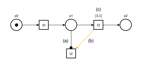
Figure 2: Petri net with mentioned extensions: (a) tokens from $p_{1}$ will not be removed when firing transition $t_{2}$; (b) transition $t_{2}$ cannot be fired if $t_{3}$ is enabled ($t_{3}$ has higher priority over $t_{2}$); (c) transition $t_{3}$ can only be fired within the time interval [3, 5] time units after it became enabled.

3.1.2 Fiacre and TINA

Fiacre [4] is a specification language for describing compositionally both the behavioral and timing aspects of embedded and distributed systems. It has a formal semantics and can be used as an input format for formal verification tools (mainly real-time model-checkers) as well as for simulation purposes.

Fiacre stems from several projects involving industrial and academics partners, and is developed at LAAS. Besides the application described in this document, Fiacre has been used in a variety of applicative domains, like telecoms, avionics and robotics systems. In this work, we use Fiacre specifications with the model-checking toolbox TINA.

Fiacre Language

Fiacre programs are structured into processes, modeling sequential activities, and components, describing a system as a composition of processes or other components. Fiacre supports the two most common coordination paradigms: by shared variable and by asynchronous message-passing.

Processes are defined from a set of parameters and control states, each associated with a set of symbolic transitions (following keyword from). The initial state is the source state of the first transition. The transitions declare how variables are updated, which events may occur, and when. They are built from standard deterministic programming constructs, non-deterministic constructs (such as external choice, operator select), communication statements, temporal constraints (construction wait) and jumps to a state (keyword to or loop).

Components are built as parallel composition of processes and/or other components (by operator par $P_{0}||...||P_{n}$ end). Compositions specify both the processes or component instances and their interactions. Shared variables and communication ports are within components. Communication ports may be associated with time constraints, applying to all interactions though those ports and with priorities. The ability to express timing constraints in programs is a distinguishing feature of Fiacre.

Introductory material and examples can be found on the Fiacre website. Also, some of the Fiacre specifications developed in this work are described later in Chapter 5.

TINA Toolbox

Tina (TIme Petri Net Analyzer) [5] is a software environment to edit and analyze enriched Time Petri Nets. The core of the Toolbox is an exploration engine generating state space abstractions; these abstractions are then fed to model-checking or equivalence checking tools. The front-end converts models into an internal representation — Time Transition Systems (TTS) — an extension of Time Petri Nets with data and priorities. A compiler, frac, converts Fiacre description into TTS descriptions, therefore enabling model-checking of Fiacre specifications by Tina.

3.2 Software-Defined Networking

Software-defined networking (SDN) [3] is an emerging networking paradigm. In an SDN, the network’s control logic (control plane) is separated from the underlying routers and switches that forward the traffic (data plane). With the separation between the control plane and the data plane, network switches become simply forwarding devices and the control logic is implemented in a logically centralized controller (or network operating system), simplifying policy enforcement and network (re)configuration and evolution.

In this work we use the network prototyping software Mininet along with the OpenFlow protocol to virtualize avionics networks, more specifically AFDX.

3.2.1 OpenFlow

OpenFlow [13] is a communication protocol that controls a switch’s forwarding behavior. It is running between a controller and multiple switches. Packets can be matched on different fields (e.g. destination MAC address) and then associated to an action or a set of actions. Actions include forwarding to ports, but also rewriting of certain parts of the packet. OpenFlow defines a rule for each flow; if a packet matches a rule, the corresponding actions are performed (e.g. drop, forward, modify, or enqueue).

3.2.2 Mininet

Mininet [8] is a system for rapidly prototyping large networks on the constrained resources of a single laptop. By combining lightweight virtualization with an extensible CLI and API, Mininet provides a rapid prototyping workflow to create, interact with, customize and share a software-defined network, as well as a smooth path to running on real hardware.

Users can implement a new network feature or entirely new architecture, test it on large topologies with application traffic, and then deploy the exact same code and test scripts into a real production network. Mininet runs surprisingly well on a single laptop by leveraging Linux features to launch networks with gigabits of bandwidth and hundreds of nodes (switches, hosts, and controllers).

Mininet uses the lightweight virtualization mechanisms built into the Linux OS: processes running in network namespaces, and virtual Ethernet pairs. Below are described the main components used by Mininet to create virtual networks.

Links: A virtual Ethernet pair, or veth pair, acts like a wire connecting two virtual interfaces; packets sent through one interface are delivered to the other, and each interface appears as a fully functional Ethernet port to all system and application software. Veth pairs may be attached to virtual switches such as a software OpenFlow switch.

Hosts: A host in Mininet is simply a shell process (e.g. bash) moved into its own network namespace. Each host has its own virtual Ethernet interface(s) and a pipe to a parent Mininet process, which sends commands and monitors output. Network namespaces are containers for network state. They provide processes with exclusive ownership of interfaces, ports, and routing tables.

Switches: Software OpenFlow switches provide the same packet delivery semantics that would be provided by a hardware switch.

Controllers: The strategic point in SDN, controllers connect and configure the network devices (routers, switches, etc.). Controllers can be anywhere on the real or simulated network, as long as the machine on which the switches are running has IP-level connectivity to the controller.

Figure 3 illustrates the components and connections in a two-host network created with Mininet.

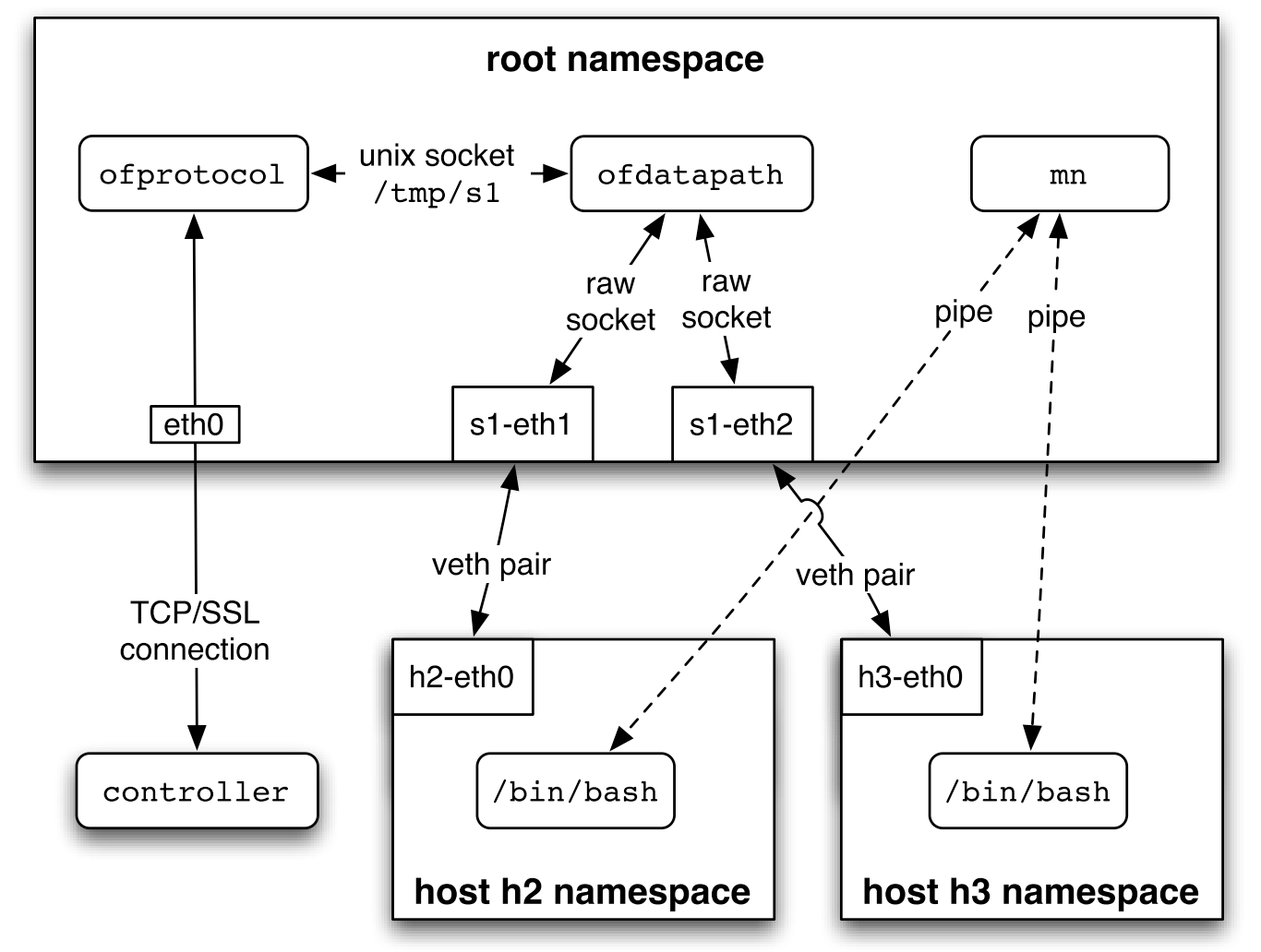
Figure 3: Two-host virtual network example created with Mininet. Mininet creates a virtual network by placing host processes in network namespaces and connecting them with virtual Ethernet (veth) pairs. In this example, they connect to a user-space OpenFlow switch. Source: Lantz et al. [8]

Mininet exports a Python API to create custom experiments, topologies, and node types (switch, controller, host, or other), which is used to create all the virtualized networks described later in this document.

3.3 Real-time Operating Systems

When operating with real-time operating systems (RTOS), reaching the desired result within the deadline is as important as reaching the result in the correct fashion. That is to say that tasks are required to be completed in time otherwise they lose their validity.

For the purpose of ensuring deadline meeting, operating systems that run in real-time are available in many different forms. Since critical systems such as avionics networks rely on determinism, the use of a real time OS with this characteristic (hard real-time OS) is the choice for this project. Hard real-time OSes are systems that can deterministically meet a deadline, meaning that a task is always finished within its time-frame and being unable to do so is considered a failure.

3.3.1 Xenomai

Xenomai is a hard real-time development framework that cooperates with the Linux kernel, providing real-time support to user space applications and at the same time seamless integration to the environment.

To support hard real-time capabilities to the Linux kernel, Xenomai implements a micro-kernel between the hardware and the Linux kernel. This micro-kernel is responsible for executing hard real time tasks and intercepts interrupts, blocking them from reaching the Linux kernel, hence preventing the Linux kernel from preempting the hard real-time micro-kernel.

Xenomai shows immense flexibility and ease of use for being Linux based, and is already being used in several projects at LAAS, hence the choice to use this real-time OS in this work.

4 Overview of the AFDX specification

This chapter describes the network protocol studied in this project. The fundamental components of the protocol are described, followed by a use case network which will be used to identify, clarify and organize the system requirements for the next chapters.

4.1 AFDX / ARINC 664

AFDX is an acronym for Avionic Full-Duplex Switched Ethernet [16], a data network for safety-critical applications that utilizes dedicated bandwidth while providing deterministic quality of service. The network is based on standard IEEE 802.3 Ethernet technology.

There are many benefits from using commercial-off-the-shelf (COTS) Ethernet components. This include reduced overall costs, faster system development and easier maintenance. However, standard commercial grade Ethernet do not meet avionics network requirements. For this reason, AFDX was defined as an extension of Ethernet standard that adds support for Quality of Service (QoS) and deterministic behaviour.

An AFDX network consists of so called End Systems and switches, where point-to-point or point-to-multipoint connections are represented by Virtual Links (VL). We explain the main concepts of AFDX networks in this chapter.

4.2 End Systems

An End System (ES) is a component connected to the AFDX network capable of handling all AFDX related protocol operations. Usually, an End System is part of an avionic or aircraft subsystem, which needs to send or receive data over the AFDX network.

This interface guarantees a secure and reliable data interchange with other avionics subsystems. One or more switches, depending on the network hierarchy, are located on the data path between two End Systems.

As shown in Fig. 4, an avionics computer system connects to the AFDX network through an End System. In general, an avionics computer system is capable of supporting multiple avionics subsystems, isolated from one another through partitioning. The End System will then multiplex the traffic from the avionics subsystems onto one single wire, and it must be capable of doing so respecting several timing constraints, some of which are discussed later in this document.

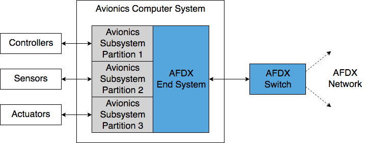
Figure 4: Example of an End System connected to different avionics subsystems.

4.3 Virtual Links

One of the precursors to AFDX is ARINC 429, a standard developed for safety-critical applications in 1977 (30 years before AFDX was patented). One of the most desirable features of an ARINC 429 connection [12] is the fact that it represents a private line between sender and recipient(s) of data. Hence the physical bandwidth of the connection is available at all times, and no concurrent transmit requests can occur. This degree of separation is mandatory when interconnecting avionics systems with different levels of criticality. On the minus side, the ARINC 429 approach means that every connection needs a dedicated pair of wires, which can be difficult to lay out on a plane and can add significant weight. AFDX achieves an equivalent result by choosing logical connections, referred as Virtual Links (VL), over physical ones. VL are based on partitioning the time at which communication can occur on a physical link.

In an AFDX network, each logical connection is represented by a Virtual Link. Each VL builds a unidirectional logic between a unique source ES to one or more target ES, thus providing a private line with bounded latency and guaranteed bandwidth. An example of Virtual Link topology is given Fig. 5, where the network has three VL, connecting six End Systems using only two switches.

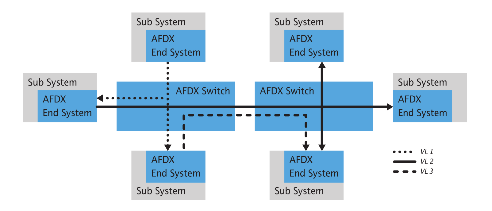
Figure 5: Virtual Link topology. Source: AFDX White paper [16]

4.4 Switch

The core of an AFDX network is built using switches, which have more responsibilities than their counterpart used in commercial Ethernet network. In addition to the obvious switching functions, an AFDX switch must perform frame filtering and traffic policing duties, ensuring that traffic arriving at the switch is compliant with the restrictions set for the appropriate VL.

In order to decouple transmit operation from data reception, all data paths use separate data buffers, thus creating true full duplex data links between End Systems. Because updating the data paths while the switch is operating introduces variable latency, which is not acceptable for avionic data networks, an AFDX switch forwards packets according to a static configuration table. The main components of an AFDX switch is shown in Figure 6.

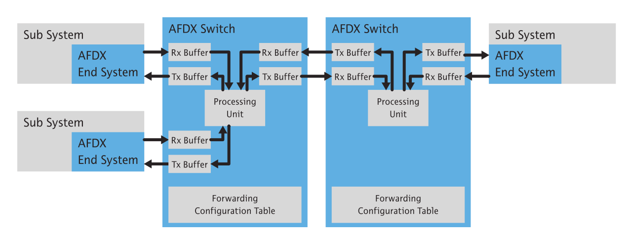
Figure 6: AFDX Subsystem to Switch communication. Source: AFDX White paper [16]

4.4.1 Traffic Policing

The AFDX standard specifies a traffic policing function at the switch based upon the token-bucket algorithm common to switched-packet networks. The goal of traffic policing is to ensure that no VL exceeds its allotted bandwidth. This algorithm will be explained in depth in the next Chapter.

4.5 Guaranteed Service

The AFDX protocol is oriented towards ensuring guaranteed service at every level; both the bandwidth and maximum end-to-end latency of the link are guaranteed. However, there is no guarantee of packet delivery. Packets may be dropped, for example, if they will exceed the limit imposed by traffic policing. Since AFDX is only concerned by the transport layer, transmission acknowledgements and re-transmissions requests must be handled at the application level.

4.5.1 BAG

The primary bandwidth control mechanism is the BAG (Bandwidth Allocation Gap) (Figure 7). The BAG defines the minimum time interval between the starting bits of two successive AFDX frames, assuming zero jitter. The AFDX specification allows for BAG values that are in the range of 1..128 ms and that are a power of $2$; that is a bag is always of the form $2^{n}$ with $n\in\{0,\dots,7\}$.

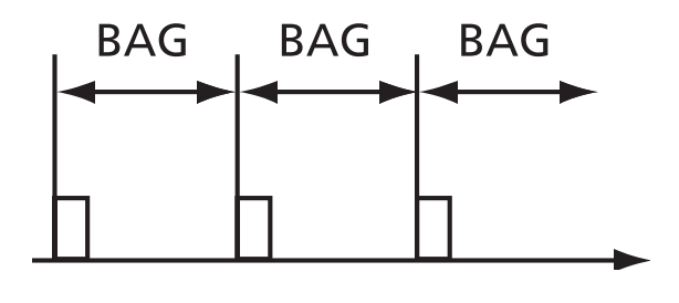
Figure 7: Bandwidth Allocation Gap. Source: Developing AFDX Solutions [1]

Each VL has an associated BAG and a maximum frame size, but a VL may not use all the bandwidth, i.e. the time between two consecutive packets may be larger than BAG. However, it may not be smaller than BAG and it is the responsibility of the ES to enforce this.

4.5.2 Jitter

The ES may introduce jitter when transmitting frames for a given VL. This jitter is defined as the delay between the beginning of the BAG and the date when the first bit of the frame is sent (Figure 8).

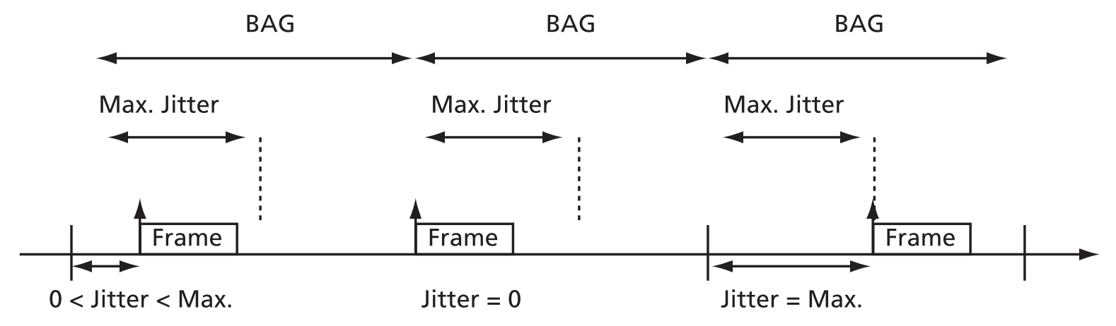
Figure 8: Jitter Defined. Source: Developing AFDX Solutions [1]

A given ES may have to transmit data for multiple VLs, so a frame from one VL can be delayed up to the maximum allowed jitter value to limit the instantaneous ES frame rate and thus accommodate frames from other VLs. The maximum allowed jitter for a given ES is defined by equation 1, below:

$$\text{Max. Jitter}\leq 40\mu s+\frac{\sum\limits_{j\in\{VLs\}}((20+Smax_{j})*8)}{\text{Nbw}}$$ (1)

$$\text{Max. Jitter}\leq 500\mu s$$ (2)

where Nbw is the link bandwidth (100 Mbps), based on standard IEEE 802.3 10/100 Mbit Ethernet hardware and equal for all VLs, and $S_{max}$ is the maximum allowed frame size for the VL (in number of bytes). As seen from equation 1, the specification allows a minimum of 40 $\mu s$ for the “technological” jitter, while the “second part” part of the formula takes into account the time needed to transfer the frames payload. In no case the total jitter can exceed a hard-limit of 500 $\mu s$, see equation 2.

4.5.3 Latency

Latency measures the time needed for a packet to travel through the network.

Although AFDX does not specify a maximum system latency, any supplier is required to specify the upper limit of latency for any system delivered.

4.6 Frame Format

The AFDX frame format is shown in Figure 9.

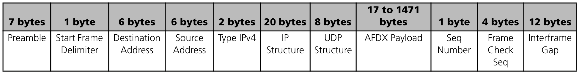
Figure 9: AFDX Frame. Source: Developing AFDX Solutions [1]

The one-byte sequence number is used to maintain ordinal integrity within a given VL. The frame sequence number is initially set to 0 upon ES start-up or reset. During continuous operation, the number wraps back to 1 after reaching a value of 255.

The maximum frame size is set for each VL and is represented by the parameter $S_{max}$. The range of this parameter is between 64 and 1518 bytes.

The destination and source addresses listed contain the MAC addresses for the ESes. AFDX network addressing is based upon the MAC addresses, which are 16-bit in length. The source address must be a unicast address and follow the format detailed in the specification, and includes bits for identifying to which of the two redundant networks the MAC is attached. The destination address is a multicast address that includes a 16-bit VL identifier.

4.7 Redundancy

An AFDX network is constructed so there are two independent paths (including MACs, PHYs, and cabling) between each ES, as well as redundant switches to protect the network from a failure at the MAC level or below. The default mode is to transmit the same frame (with identical frame sequence numbers) across both networks, but the redundancy option can be configured so that frames for a given VL may be sent along either or both of the networks.

The redundancy management is done at application level. The receiving ES then accepts the first valid frame and passes it to the application. Once a valid frame is received, any other frame with the same sequence number is discarded.

4.8 Use Case: Flight Management System

We have used several example of AFDX networks to benchmark our approach. While most of them are generated randomly, we have also used a representative example of network extracted form the PhD thesis of Michael Lauer [9], which is a subset of the navigation system, called Flight Management System (FMS), of an Airbus plane. The purpose of this system is to control the display of navigation information on the flight screens used by the pilots. We detail this network since it gives a good idea of the typical complexity of an “avionic function”. A plane usually operates a thousand such functions.

The architecture of the FMS is composed of a set of modules interconnected through an AFDX network. This architecture is shown in Fig. 10. Seven modules, from Module 1 to Module 7, are used to host the avionics functions. The Remote Data Concentrators ($RDC_{1,2}$) connect the pressure sensors ($sensor_{1,2}$) to the network. Each of these modules contain an End System responsible for handling all AFDX related protocol operations. The keyboards ($key_{1,2}$) and displays ($display_{1,2}$) however are connected directly to the modules via a field-bus. The AFDX network consists of five switches, S1 to S5, represented by the purple boxes in the figure.

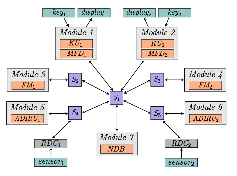
Figure 10: Flight Management System network architecture. Source: Lauer [9]

Table 2 shows the configuration for each VL of the network.

Table 2: FMS Virtual Links.

VL	source	destination	BAG (ms)	$S_{max}$ (bytes)
$VL_{1}$	$KU_{1}$	$FM_{1},FM_{2}$	32	75
$VL_{2}$	$KU_{2}$	$FM_{1},FM_{2}$	32	75
$VL_{3}$	$FM_{1}$	$MFD_{1}$	8	625
$VL_{4}$	$FM_{1}$	$NDB$	16	125
$VL_{5}$	$FM_{2}$	$MFD_{2}$	8	625
$VL_{6}$	$FM_{2}$	$NDB$	16	125
$VL_{7}$	$NDB$	$FM_{1}$	64	500
$VL_{8}$	$NDB$	$FM_{2}$	64	500
$VL_{9}$	$RDC_{1}$	$ADIRU_{1}$	32	64
$VL_{10}$	$RDC_{2}$	$ADIRU_{2}$	32	64
$VL_{11}$	$ADIRU_{1}$	$FM_{1},FM_{2}$	32	87.5
$VL_{12}$	$ADIRU_{2}$	$FM_{2},FM_{1}$	32	87.5

This network will be used extensively during this document as basis for modeling, virtualization, simulation and benchmarking. However, this topology is only a small part of a full network system and is considered to be small to industry standards. Indeed, a typical industrial AFDX network can have more than 100 ES, two redundant sub-networks with 8 switches each, with thousands of VLs (more than 6000 paths) on each sub-network. In order to test the scalability of our tools, we will often use variations of this use-case where case network topology and parameters are tweaked when applicable to represent different, more realistic scenarios.

4.9 Benchmarking

I have developed two generators of AFDX networks (specifications) in order to validate and to benchmark our virtualization framework. The first generator is used to build a simple AFDX network with $N$ Virtual Links, such that: all the VLs have only one source and one destination; the bag and the frame size of each VL is chosen randomly; and all the VLs go through a single (shared) router. The idea is to generate a new, random network topology by varying the following three parameters:

• Number of Virtual Links: this is the main factor that drives the complexity of the network. The VLs are generated as point-to-point links connected to a single switch.

• BAGs: for each VL the emission period is chosen from the set of available BAGs {1, 2, 4, 8, 16, 32, 64, 128}$ms$.

• Frame size: frames emitted on the VLs can be of any size between 64 and 1518 bytes. For each VL, the frame size is constant throughout the simulation

In addition to randomly generating the topology, some simulation parameters can also be arbitrarily chosen to cover a bigger spectrum of network behavior:

• Speed factor: slows down or speeds up the network emission periods. For example, a speed factor of 2 will make all the VLs send frames twice as fast.

• Duration: the simulation duration, where we consider short to be 10 seconds, medium 60 seconds (1 minute) and long 300 seconds (5 minutes). Since the emission period is in the order of milliseconds, even the shorter duration produces a considerable amount of traffic.

I have also developed a second kind of generator based on templates. The idea is to start from a known network (expressed in a CSV file, see for example Listing 9) and to generate bigger version by taking several copies of it. Network specifications can be saved using a textual formats and reused with the different tools that we developped during my internship.

By looking at the traffic over time, more specifically the jitter and latencies of each Virtual Link, a detailed analysis of the network can be accomplished. This information yields how the traffic over the network is shaped—who may be transmitting data at a higher rate than configured, or whose traffic is the most affected by the current configuration.

While studying the time series of the traffic provides a simple yet informative visualization of the network dynamics, they are not very practical for studying finer-scale features. Traces can become long enough that in small scales any plot is dominated by over-plotting, and does not provide much useful information. This is specially true when comparing two time series that are already rather similar. In this dissertation we make use of an alternative method called Cumulative Distribution Function (CDF), which enables the analysis and comparison of traces at finer scales.

Figure 11 illustrates an empirical example of a CDF plot. This plot means that a relative amount of $F(x)$ values from the given set of numbers used to calculate this distribution are less or equal than the value $x$.

Figure 11: Empirical CDF plot. Source: http://www.andata.at

This plot enables a direct quantitative reading of relevant key values. For example, the minimum can be seen right at the point where the CDF begins and hits the x-axis—i.e. zero probability of having values that are smaller than $F(x)$ when $x=0$. Similarly, the maximum can be seen where the CDF reaches the line $y=1$ and ends. Percentiles can also be read directly from the x-axis. The existence of outliers also becomes apparent, and it is showcased later through some experimental results.

5 Three Formal Models of AFDX Networks

This section discusses the modeling of the main components of an AFDX network using the formal specification language Fiacre (see Section 3.1.2). We describe three different abstractions that corresponds to different levels of precision on how frames are transported across the network. In doing so, we also define a formal model of the token bucket traffic policing mechanism. We conclude by giving some experimental results obtained from simulation of these models. These formal models are the first contribution of this work.

5.1 Modeling with the Fiacre language

We model the behaviour of an AFDX network using three different approaches: (1) timed channels; (2) direct virtual links; and (3) switched virtual links. Instead of defining the complete encoding of a whole network, we consider only the model of a single Virtual Link, that is Virtual Link 1 ($VL_{1}$) of the FMS example given in Sect. 4.8. Since Fiacre supports composition of processes and components to create more complex models, we can easily build the whole network from this simple example.

Virtual Link 1 is used to transport frames from the Keyboard Unit partition $KU_{1}$ on Module 1, to both Flight Manager partitions $FM_{1}$ and $FM_{2}$ on Modules 3 and 4, respectively. Since we consider frames with a minimum-sized payload of $17$ bytes, we can derive the following properties from Table 2 and equation (1):

• BAG = 32 ms. The minimum time between two consecutive frames.

• J_max = 47.6 $\mu$s. The maximum amount of jitter introduced by the End System.

• S_max = 75 bytes. The maximum frame size transmitted on this VL.

We focus our model on the network part of the system. Therefore we do not model the behaviour of End Systems and simply assume that each VL transmits with maximum bandwidth, meaning that every frame has a constant size and is sent by the ES exactly at each BAG.

We start with the model of a simple periodic communication protocol, see Listing 1. This example has two communicating process instances (Sender and Receiver) encapsulated in a component (System) which defines the communication port and the timing constraints. For example, channel p is declared with a timing interval of $[32,32]$, meaning that every interaction (synchronization) on this channel must be performed exactly 32 units of time after the two processes are willing to communicate.

In Fiacre, the expression p! send stands for an emission on port p, carrying the value of variable send. Symmetrically, the expression p? x stands for a reception on port p; the value “carried” by the port is assigned to variable x. We can view each of our encodings of AFDX as a more refined example of this simple system.

⬇

process Sender [pout : int] is

states send

var msg : int $:=$ 0

from send

pout! msg; to send

process Receiver [pin : int] is

states recv

var msg : int

from recv

pin? msg; to recv

component System is

port p : int in [32, 32]

par p in

Sender [p]

$\parallel$ Receiver [p]

end

Listing 1: Example of sender and receiver system on Fiacre.

5.1.1 Timed Channel

The first network approximation model is based on components called timed channels. The idea is that the whole “travel” of a frame through the switches and data buffers of the actual network can be abstracted away as a simple delay on a dedicated channel. In the encoding of a whole network, we simply associate one timed channel to each path in a VL. Hence each channel represents a link between a single sender and a single receiver.

A timed channel is characterized by a time interval $[a,b]$, where $a$ and $b$ are the best (lowest) and worst network traversal time for a frame in a given VL, also known as Worst Case Traversal Time (WCTT) and Best Case Traversal Time (BCTT). The traversal time corresponds to the sum of the technological latencies of the switches crossed along the path and the output transmission time for each of these devices. These bounds can be calculated using techniques such as Network Calculus [10] or Trajectory Approach [11].

Figure 12 shows a diagram of how this approximation is applied to Virtual Link 1. $VL_{1}$ is decomposed into two timed channels, $C_{1}$ and $C^{\prime}_{1}$, each one transmitting frames every 32 ms (BAG) with a delay in the interval $[298,444]$ (here the unit of time is the $\mu$s). The full use case network architecture with timed channel approximation and the corresponding parameters are given on Appendix A.

Figure 12: Timed channels approximation of $VL_{1}$.

Listing 2 illustrates the timed channel process which acts as the communication medium between the communicating processes. The sender process writes a new frame into variable vin every BAG ms, meaning that the value of vin becomes different from NIL; then, as soon as this condition is true (the Fiacre keyword on is used to define a guard on a transition), process TimedChannel waits for a delay in the interval $[298,444]$ then copies the frame to vout and resets vin to NIL so it can wait for the next frame; finally the receiver process reads the frame from the vout variable whenever there is a frame available.

⬇

type Frame is NIL | VALUE end

process TimedChannel (&vin, &vout : Frame) is

states get

from get

on (vin <> NIL);

wait [298, 444];

vout $:=$ vin;

vin $:=$ NIL;

to get

Listing 2: Fiacre model of timed channels.

It is worth noting that network traversal times are always smaller than the period at which frames are generated (the BAG). This holds true for the other timed channels as well (see Table 3). This means that a timed channel will always delay only one frame at a time, which greatly simplifies our model. Also, this first implementation does not take into account the jitter at the sender process. However, the following models takes into account jitter and it would be easy to adapt the same approach in this case also.

5.1.2 Direct Virtual Link

In our second approach, we take into account the multicast nature of Virtual Links as if they were direct links between the sender and receivers partitions, but without including the switches.

Each VL is composed by a unique sender process (in contrast to one for each timed channel), and one or more receiver processes. As shown in Figure 13, $VL_{1}$ originates from one port at partition $KU_{1}$, and is synchronized to both destinations $FM_{1}$ and $FM_{2}$.

Figure 13: Approximation of $VL_{1}$ behavior without the switches.

We should not model this approach as is. Indeed, if we are not careful, and since receivers are synchronized directly with the same sender, both would receive the frames at the same time. This is obviously not true in a real network since traversal time can vary on different paths. One way to introduce different traversal time for each path is to make the receiver (Rx) be a composition of two different processes, here called RxPort and RxDelay as shown by Listing 3. Process RxPort is synchronized with the sender by the communication port pin, but we do not consider the reception of a frame complete by this process. Instead, it sends the frame to RxDelay using a shared variable, which will introduce a variable delay to only then mark the frame as received.

⬇

type Frame is NIL | VALUE end

process RxPort [pin : Frame] (&frame : Frame) is

states recv

from recv

pin? frame; to recv

process RxDelay (&frame : Frame) is

states idle, delay

from idle

on (frame <> NIL); wait [0, 0]; to delay

from delay

wait [BCTT, WCTT]; frame $:=$ NIL; to idle /* frame received */

component Rx [pin : Frame] is

var frame : Frame $:=$ NIL

par pin in

RxPort [pin] (&frame)

$\parallel$ RxDelay (&frame)

end

Listing 3: Fiacre model of the VL receiver component (Rx).

The Tx component has a similar mechanism to introduce jitter on frame emission. It is a composition of a TxBAG process, which sends frames through a shared variable to a TxJitter process, who then introduces a bounded delay corresponding to the VL’s maximum jitter specification before sending the frame on the communication port. Since the hard limit for the maximum admissible jitter is 500 $\mu$s (EQ. 2), which is smaller than the lowest BAG (1 ms) (see Sect. 4.5.1), we do not have to worry about TxJitter having to delay more than one frame at a time.

5.1.3 Switched Virtual Link

Our last modelling approach is the closest one to the actual physical behaviour of the network. In particular, it takes into account switches and the routing of frames until they reach their destination.

In this approach, each partition is synchronized to a switch through input and output communication ports. The switches are configured with a static routing table that will forward the frames to the correct output ports. Figure 14 shows this concept applied to $VL_{1}$, where we see that each channel goes through two distinct pair of switches.

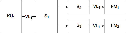
Figure 14: $VL_{1}$ with the switch model. The switches forward the frames from the sources to its destinations.

Since we do not model the traffic shaping mechanism from the End Systems, which combines different VLs into one single connection, we still need separate ports for each VL originating on the same partition.

This model provides the possibility to specify hardware constraints and allows for a more detailed implementation of the AFDX behaviors. For example, one of the most important is the traffic policing mechanism present at the switch which provides guarantee on the bandwidth for every VL.

Modeling the traffic policing contraption with formal methods adds flexibility when integrating the network model with real or virtualized systems. Because this algorithm has some properties that are not trivial to model in Fiacre, such as maintaining a continuous account, the next section is dedicated to it since it is a major part of this work’s contribution.

5.2 Traffic Policing

AFDX specifies a traffic policing function at the switch based on the token bucket algorithm, that is common to many packet-switch networks. The goal of traffic policing is to ensure that no Virtual Link exceeds its allotted bandwidth.

The specification requires the use of one or both of the following two algorithms for traffic policing:

• Byte-based policing

• Frame-based policing

As shown in [18], the byte-based token bucket algorithm may not be able to perform the traffic policing as expected. Therefore, frame-based policing was chosen for this implementation.

5.2.1 Frame-based Token Bucket Algorithm

The token bucket filter implements a resource-based algorithm to decide whether to accept or reject a frame. The concept is quite simple. A bucket has a current balance that cannot be negative. The bucket is credited as time progress but cannot exceed a maximal value. Each accepted frame has a cost, deducted from the bucket and a frame is allowed only if the current balance is high enough.

In an AFDX network, each VL has an independent bucket that is controlled by the first switch found coming out of the source ES. For a given $VL_{i}$, an account $AC_{i}$ is maintained and credited with tokens (in bytes) at the following rate:

$$S_{i}^{max}/BAG_{i}$$ (3)

where $S_{i}^{max}$ is the maximum allowed frame size and $BAG_{i}$ is the Bandwidth Allocation Gap for the $VL_{i}$. From the AFDX standard, tokens accumulate in the account ($AC_{i}$) until it reaches a limit value of $AC_{i}^{max}$, such that:

$$AC_{i}^{max}=S_{i}^{max}*(1+J_{i}^{max}/BAG_{i})$$ (4)

where $J_{i}^{max}$ is the maximum defined jitter value for VL number $i$.

Assume a frame of size $S_{i}$ is emitted on $VL_{i}$. When it arrives at the first switch, it is allowed if the current account value, $AC_{i}$, is greater than $S_{i}^{max}$. In this case $AC_{i}$ is decremented by $S_{i}^{max}$. If the frame account $AC_{i}$ is less than $S_{i}^{max}$, the frame is rejected and the value of $AC_{i}$ is left unchanged. Figure 15 illustrates this behavior.

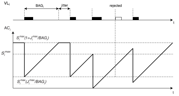
Figure 15: Example of frame-based traffic policing

5.2.2 TPN Model

On the face of it, the behaviour of the token bucket seems difficult to model. Indeed, the time at which a new frame is allowed may depend on the time the previous frame was seen. Which indicates that we may be faced with a system that has an hysteresis; an hybrid system. Surprisingly, it is possible to model frame-based policing using an ordinary Time Petri Net (TPN). The model if given in Fig. 15. The idea is to consider four possible cases, each represented by a different state (or place in this case), s0 to s3.

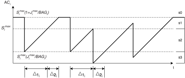
Figure 16: Frame-based policing parametrization to model as TPN

Place s0 is used to model a state where the token bucket has reached its maximal value, as shown in Fig. 16. This is also the initial state of the system. Place s1 corresponds to a state where a frame arriving at the switch will be accepted. In between these two states, we use places s2 and s3 to represent the transient state where frame can be rejected. The bucket is associated with two time constants, $\Delta_{1}$ and $\Delta_{2}$, that correspond, respectively, to the time needed for the bucket to accept a frame after “leaving” state s0 and the time needed for reaching its maximal balance. Place s2 is used when a new frame can be accepted less than $\Delta_{1}$ in the future. Place s3 is used when a frame is accepted before the bucket reached its maximal value.

As the account $AC_{i}$ for a Virtual Link $VL_{i}$ is credited at rate $J_{i}^{max}/BAG_{i}$ (EQ. 3), the values of $\Delta_{1i}$ and $\Delta_{2i}$ are defined by:

$$\Delta_{1i}=(S_{i}^{max}-S_{i}^{max}*\frac{J_{i}^{max}}{BAG_{i}})*\frac{BAG_{i}}{S_{i}^{max}}=BAG_{i}-J_{i}^{max}$$ (5)

$$\Delta_{2i}=[S_{i}^{max}*(1+\frac{J_{i}^{max}}{BAG_{i}})-S_{i}^{max}]*\frac{BAG_{i}}{S_{i}^{max}}=S_{i}^{max}*\frac{J_{i}^{max}}{BAG_{i}}*\frac{BAG_{i}}{S_{i}^{max}}=J_{i}^{max}$$ (6)

Figure 17 shows an example implementation of the frame-based token bucket policing applied to a VL with $BAG=8$ and $J_{max}=2$ time units. These values were chosen in order to simplify calculations and ease understating, but they do not represent a real VL configuration.

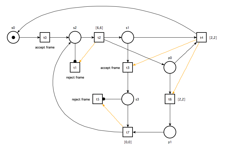
Figure 17: Frame-based token bucket for VL with $BAG=8$ and $J_{max}=2$

Because we need to keep track on how much time has elapsed when accepting frames while on place s1—time that is necessary to transition back from s3 to s2—we need to add two additional places: p0 and p1. This behavior simulates the token bucket account increasing with an steady rate, where accepting frames leaves the account in a state proportional to how "filled" it was before.

Priorities here are necessary mainly because of the ambiguity when transitioning from accepting- to rejecting-states and vice versa. Since the frame accepting policy is based on comparing its size to how much tokens—normally represented by bytes—is available on the account, when the right amount of time has elapsed equivalent to the frame size, the algorithm dictates that it must be accepted. Thus we prioritize accepting frames over rejecting right at the state boundaries, when appropriate. Furthermore, owing to the way we model the keeping of time from state s1, the two rightmost priorities ensure the proper transition to state s0 when the account is full.

5.2.3 Fiacre implementation

We can define a Fiacre specification that is equivalent to the TPN given in the previous section. To implement this TPN model in Fiacre, a composition of two processes is necessary. Figure 18 display the two processes, TB1 and TB2 , which are synchronized in transitions t0, t1 and t2 to create the full model TokenBucket. Transition times d1 and d2 correspond to $\Delta_{1}$ and $\Delta_{2}$ respectively.

Figure 18: Fiacre processes that compose the frame-based token bucket TPN model.

The full Fiacre code to implement this model is listed on Listing 4. This code does not have means of directly integrating with external components (e.g. sender and receiver), since the communication port frame is local to the TokenBucket component and it is only used to flag the arrival of frames, but it showcases the algorithm mechanism and gives a full, neat example on how a TPN is translated to the Fiacre specification language.

⬇

process TB1 [t0, t1, t2, frame : sync] is

states s0, s1, s2, s3

from s0

frame; to s2 // accept frame

from s2

select

frame; loop // reject frame

[] t0; to s1

end

from s1

select

frame; to s3; // accept frame

[] t1; to s0

end

from s3

select

frame; loop // reject frame

[] t2; to s2

end

process TB2 [t0, t1, t2, t3 : sync] is

states s0, s1, s2

from s0

t0; to s1

from s1

select

t1; to s0

[] t3; to s2

end

from s2

t2; to s0

component TokenBucket is

port

t0 : sync in [d1, d1], // d1 = BAG - Jmax

t1, t3 : sync in [d2, d2], // d2 = Jmax

t2 : sync in [0, 0],

frame : sync // frame reception

priority

t1 > t3,

t0 | t1 | t2 | t3 > frame

par * in

TB1 [t0, t1, t2, frame]

$\parallel$ TB2 [t0, t1, t2, t3]

end

Listing 4: Token bucket algorithm in Fiacre.

5.3 Experimental Results

We developed a tool to generate traces from the simulation of formal models. It is based on the stepper simulator play, which comes with the TINA Toolbox and allows the simulation step by step of net descriptions in several formats, including Time Transition Systems (TTS). Our tool loads the net and randomly advances the time, firing transitions in no particular order as they become enabled. To generate the traces, we can specify the transitions of interest in order to obtain the date at which they are fired.

While all levels of abstraction can be simulated, this report only present results from the most complex one: switched virtual links. I modeled the whole use case network—complete with all switches, End Systems and traffic policing—using the concepts described in this section. Figure 19 shows the latency of four VLs obtained from a 60-seconds simulation of the whole network.

Figure 20 illustrates the latency CDF calculated from this simulation. We can see from these graphs a similarity between Virtual Links due to the redundancy present on AFDX configurations—$VL_{1}$ and $VL_{2}$ have the same parameters and cross the same number of components when traversing the network.

The simulation to real time ratio achieved by this tool is 1:1, meaning that our simulation runs at the same speed as a real network. Latency is introduced in these simulations by changing model parameters such as the switch’s output processing time, chosen arbitrarily in this case to be 0.1 $\mu$s at maximum.

Figure 19: Latency trace for four VLs during simulation from formal models.

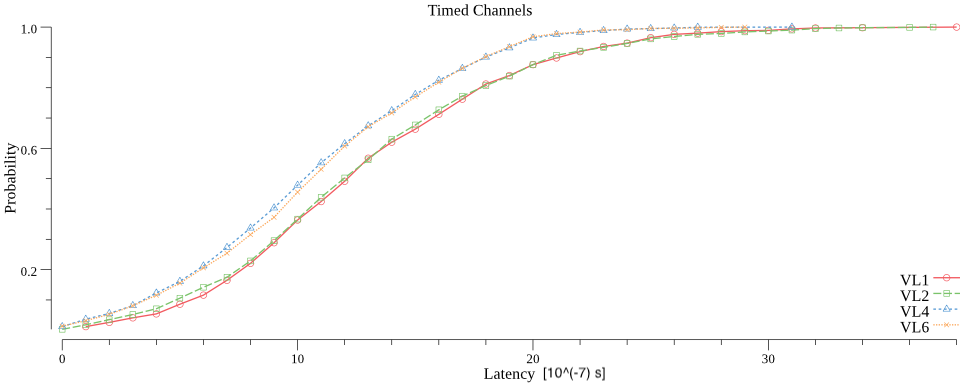
Figure 20: Latency CDF for VLs simulated from formal models.

6 Virtualization of AFDX Network

This chapter details the development and implementation of the prototype middleware for our network virtualization tool. Firstly, the main components developed to work with the Mininet framework are described, followed by how we implement the traffic policing mechanism on the Linux platform. Secondly, several experimental results are analyzed, and a strategy to circumvent some of the problems encountered is outlined.

6.1 AFDX Virtualization with Mininet

We already introduced Mininet in Section 3.2.2. Mininet creates a virtual network by placing host processes in network namespaces and connecting them through virtual Ethernet (veth) pairs connected, for example, to a user-space OpenFlow switch.

In this chapter, we use the concepts learned during the modelling of AFDX networks and the different approximations that we used for our formal models to create a virtual AFDX network based on Mininet. We analyse the viability of this approach and show ways to improve the simulation of a network.

6.1.1 Hosts

We use the concept of Hosts to represent End Systems in AFDX. Since this work focuses on implementing the network behaviours, we simplified some of the mechanisms on the application level: hosts represent the end-points of a Virtual Link; for a given VL with one source and $K$ destinations there is $K+1$ (Mininet) hosts: one for the source—responsible for sending frames—and one for each target ES—the receiver hosts.

Sender Hosts

In each of the sender hosts, throughout the simulation, a task sends frames through its veth interface periodically with respect to the VL’s BAG in order to generate its average bandwidth, as illustrated in Listing 5.

The periodic tasks are simulated using a high resolution timer with Linux soft real time scheduling, and the tasks are given the highest execution priority ($99$).

Due to a limitation of virtual Ethernet devices and Precision Time Protocol (PTP) Linux driver, timestamping at emission is done in the host node just before writing the frame into the socket.

⬇

/* Set high priority */

/* Configure socket */

/* Build AFDX frame */

for (int i = 0; i < COUNT; i++) { // send COUNT frames periodically

add_seqno(&frame); // add sequence number to frame

clock_gettime(CLOCK_REALTIME, &ts); // get timestamp

sendto(sockfd, frame, ...); // send frame on socket

nanosleep(BAG * 1000000); // wait BAG milliseconds

}

/* Save timestamps to file */

Listing 5: C code of the task running at sender host nodes (simplified).

Receiver Hosts

Similar to the sender hosts, each VL destination is represented by a task which is listening to frames arriving at its veth interface throughout the simulation, as shown in Listing 6.

At reception, frames are (software) timestamped using the PTP Linux driver, which is more precise than the way timestamping is done at emission. This difference in timestamping mechanisms may compromise the data when calculating network metrics such as latency, but is still sufficiently precise to serve its purpose.

⬇

/* Configure socket */

for (int i = 0; i < COUNT; i++) { // receives COUNT frames

recvmsg(sockfd, &frame); // receive frame on socket

/* Apply system macros for accessing the ancillary data */

memcpy(&ts, CMSG_DATA(cmsg), ...); // get software timestamping from frame

}

/* Save timestamps to file */

Listing 6: C code of the task running at receiving host nodes (simplified).

6.1.2 Switch

At the OpenFlow switch where all the hosts are connected through virtual Ethernet pairs, we use the concept of flows to implement frame forwarding.

The matching of VLs is based on the frame’s destination MAC address. OpenFlow allows for exact and wildcard matching of destination MAC addresses. To separate the flows from each other, an exact matching entry for each MAC address is needed. To allow for AFDX’s multicast behavior, multiple actions can be associated to each entry, e.g. by having multiple output actions.

This configuration must be done prior to beginning the network simulation. Openflow allows for installation of rules during the runtime of a switch. However, such behavior is not desired in avionics, especially not during flight. Therefore, we assume the installation of rules is only performed during a maintenance phase on ground and then leave all configuration as-is until the next maintenance.

Listing 7 illustrates how the flows are configured on the OpenFlow switch using the Mininet Python API. Each flow contains the input port in which the Virtual Link enters the switch, the Ethernet destination address to match the rule (Virtual Link ID), and the outputs to forward the matched VL’s packets to. With all the flows defined, we use the dpctl utility tool to add them to the flow table.

⬇

# list containing all flows

self.flows = [{"in_port": 1, # input port

"vl_id": "00:01", # virtual link ID

actions: "2,3"}, ... ] # output ports

# forwarding table rules

fwd_afdx_port = "\"table=0

␣␣␣␣␣␣␣␣␣␣␣␣␣␣␣␣␣in_port=%d

␣␣␣␣␣␣␣␣␣␣␣␣␣␣␣␣␣dl_dst=03:00:00:00:%s/ff:ff:ff:ff:ff:ff

␣␣␣␣␣␣␣␣␣␣␣␣␣␣␣␣␣actions␣=%s\""

# add forwarding rules for each flow

for flow in self.flows:

self.dpctl("add-flow", fwd_afdx_port % (flow["in_port"],

flow["vl_id"],

flow["actions"]))

Listing 7: OpenFlow switch configuration with Mininet Python API

Traffic Policing

To implement the traffic policing on the switch we use linux traffic control (tc). Traffic control is part of the linux iproute2 package which allows the user to access networking features.

With tc it is possible to attach queuing disciplines (qdiscs) to network interfaces. Queueing disciplines are packet queues with an algorithm that decides what to do with ongoing or incoming packets. In every network interface there is an ingress qdisc which works on incoming traffic. Therefore, in order to classify and police frames entering on a switch veth interface corresponding to the VL parameters, one need to add a token bucket algorithm to the ingress qdisc—this can by done by adding filters with a police action attached to it.

The filter provides a convenient mechanism for gluing together several of the key elements of traffic control. The simplest and most obvious role of the filter is to classify packets. One of the most common classifying mechanisms is the u32 classifier. The u32 classifier allows the user to select packets based on attributes of the packet. In order to classify differently for each VL, we use the u32 classifier to match according to the destination MAC address of the AFDX Ethernet frame, which contains the VL identifier.

The police action allows to limit bandwidth of traffic matched by the filter it is attached to. From the algorithms available to measure the packet rate, we use the token bucket which is configured using the rate, burst, overhead and conform-exceed parameters.

• rate: The maximum traffic rate of packets passing this action. Those exceeding it will be treated as defined by the conform-exceed option. This can be calculated for each VL by $S_{i}^{max}/BAG_{i}$ (EQ 3).

• burst: Set the maximum allowed burst in bytes. For $VL_{i}$, the burst parameters sets the amount o acceptable jitter, and can be calculated by $S_{max}*(1+J_{i}^{max}/BAG_{i})$.

• overhead: Account for protocol overhead of encapsulating output devices when computing rate. For Ethernet frames, the overhead parameter is 14 bytes.

• conform-exceed: Define how to handle packets which exceed the configured bandwidth limit. This is configured to drop in order to be compliant with the AFDX specification.

Below is an example command to add traffic control to a virtual Ethernet interface from the switch (s1-eth0) receiving frames from $VL_{1}$ (03:00:00:00:00:01), which has parameters BAG = 32 ms, S_max = 75 bytes and J_max = 0.5 ms.

  $ tc qdisc add dev s1-eth0 ingress
  $ tc filter add dev s1-eth0 parent ffff: \
        match ether dest 03:00:00:00:00:01 \
        police rate 2344bps burst 77b overhead 14 conform-exceed drop

6.1.3 Topology

To create the topology of the AFDX network we apply a many-to-one mapping to the real topology, that is we use a single switch to configure the path of all VLs. This can be thought as implementing the Virtual Link approximation presented on Chapter 5.1.1 with a single intermediate switch to perform traffic policing and create the point-to-multipoint connections for all the VLs, so we can characterize each path as a timed channel. Figure 21 illustrates this mapping applied to $VL_{1}$.

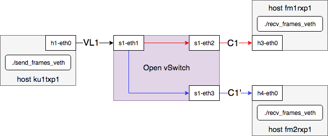
Figure 21: Many-to-one mapping applied to $VL_{1}$

6.2 Monitors

To gather information about the virtualized network performance, we have implemented three different monitor: one for checking whether the observed latency is out of bounds (with respect to the AFDX specification); a second for checking the value of jitter at emission (to detect if the sending site does not respect its realtime constraints); and finally a monitor to compute the number of frames dropped due to the traffic policing mechanism. Monitors implement a kind of runtime verification that could allow us to tag the frames that are outside the normal behaviour of the simulated network (and hence that should be disregarded in the simulation).

The timestamps referred in this document correspond to Unix time with nanoseconds resolution, and are computed with a different technique at emission and reception sites, as discussed in the previous section.

6.2.1 Latency

The latency monitor is used to verify if the network traversal time for frames on each VL path is conform with the Best (resp. Worst) Case Traversal Time (see Table 3).

In order to calculate the latency on-line (during the network simulation), the timestamp at emission is encapsulated by the payload before writing the frame into the socket. Therefore, when a frame is received by a destination process, the reception timestamp is then subtracted from the emission timestamp parsed from the payload to obtain the latency.

If the latency is greater than the WCTT for the corresponding path (timed channel), the frame is flagged and saved to a buffer, which will be dumped into a log after the end of simulation for further analysis. If the latency is smaller than the BCTT it means that we can run the simulation faster than the real network.

6.2.2 Jitter

When generating frames in the sender processes, the period BAG is not strictly respected, since the tasks need processor time which is shared among the other processes running on the machine. Consequently, a technological jitter is introduced to the BAG.

To calculate the jitter, the emission timestamp for each frame is compared with the theoretical emission time if the BAG was always strictly respected.

Say the jitter of the $i$-th frame is calculated. We classify the jitter according to four categories:

1. Too early: the frame was emitted before its normal period, that is before date $i*BAG$.

2. OK: the frame was emitted in the acceptable interval $[i*BAG,i*BAG+J_{max}]$.

3. Too late: the frame was emitted after the maximum admissible jitter $J_{max}$ but it did not missed the period (it is sent before date $(i+1)*BAG$).

4. Skipped Period: The frame has missed its period; that is it was emitted more than $BAG$ ms after date $i*BAG$.

6.2.3 Traffic Policing

To check how many frames are being dropped by the traffic policing mechanism, we use the sequence number present on the AFDX frame.

Each frame has a one-byte sequence number that increments with every frame sent. From discontinuities on the sequence number parsed at reception, we can infer the number of frames lost in transmission.

6.3 Experimental Results

The experiments are done on a Virtual Machine running Linux (1 CPU, 2048MB Memory) on top of a standard MacBook Pro laptop (Intel Core i5, 8GB Memory), using Mininet.

By analyzing the network traffic on multiple network configurations, mainly link latency and emission jitter, a number of problems emerged and modifications on the code and experimental setup became necessary to eliminate or mitigate the most relevant ones.

The rest of this chapter describes the virtualization framework evolution, explaining the reasoning behind solving the main obstacles encountered during development. For brevity, I only display the results related to the use case network configuration, but the benchmarking tools described in Section 4.9 are extensively used to generate different configurations, stress the platform and analyze its performance.

6.3.1 Pure Mininet

Right from the first experiments it is possible to notice an irregular behavior at beginning and end of simulation. This happens because Mininet takes some time to setup the network at startup, and similarly at the end when the components start to be cleaned. This behavior can be expected and we took the straightforward approach to solving it, which is to neglect the first and last 10% of simulation when analyzing the data.

Figure 22 shows the latency of all VLs of the use case network topology obtained from a 60-seconds simulation. The x-axis in this plot represents the timestamp during simulation when a frame has been emitted by a sender process (in seconds), while the y-axis shows the network traversal time that each respective frame took to reach its destination (in microseconds), for all configured paths, calculated by the latency monitor.

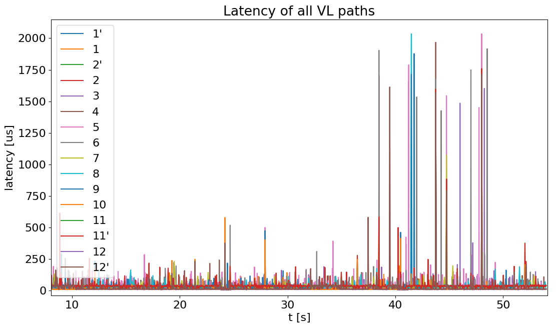
Figure 22: Latency of all VL paths.

In all simulations there are significant peaks in latency. Upon finer inspection (e.g. Figure 23) we can see that it occurs with several VLs in an orderly fashion. One plausible explanation is that other services running on the OS are stalling the execution of the processes and releasing them at virtually the same time, which gives this flush-like characteristic. Since these experiments are done in a Virtual Machine, there are aspects of the underlying system that are not well-defined, and we assume that this kind of behaviour will disappear once we run on a laptop running a native Linux environment.

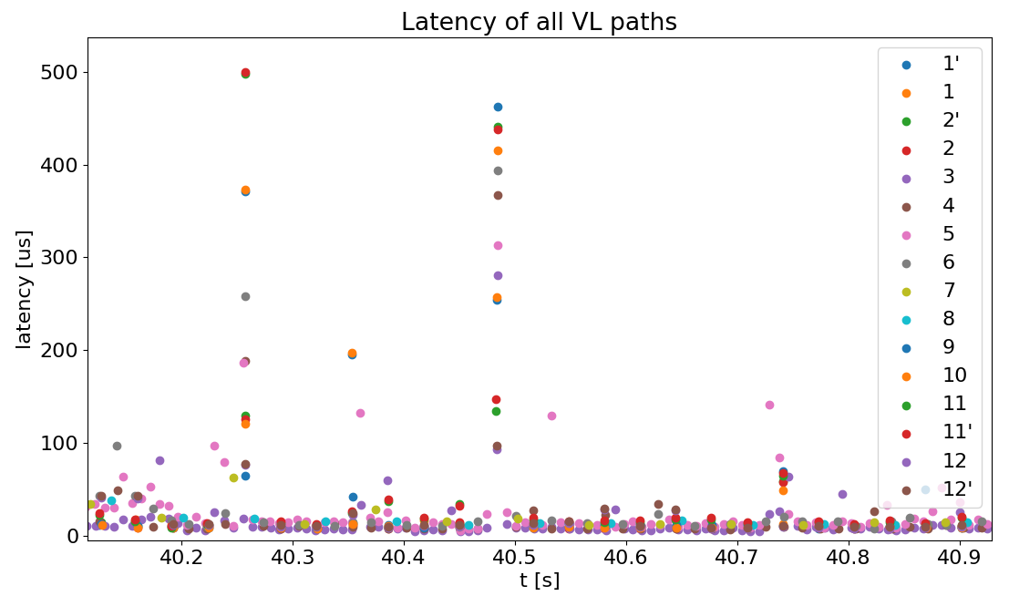
Figure 23: Latency peaks in several VL paths.

Another issue appeared when analyzing the jitter at frame emission, where it becomes evident that the periodicity dictated by the BAG is not being respected. Figure 24 illustrates the emission jitter of all VLs being accumulated as time advances. This accumulation of jitter is due to the way the periodic behavior of sender hosts is implemented. As shown in Listing 5, the emission period is simulated by freezing execution for BAG $ms$ with nanosleep() before sending the next frame. As the tasks leading to the next sleep cycle are not instantaneous, the delay introduced in each period accumulates throughout execution. To counteract this unwanted behavior, we make use of the real-time Xenomai framework to implement the sender processes as a real-time periodic task.

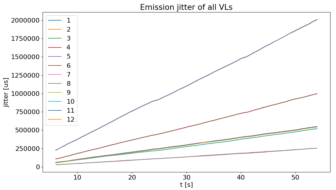
Figure 24: Emission jitter accumulating on all VLs.

6.3.2 Xenomai Periodic Task

Listing 8 shows the code necessary to integrate the real-time capabilities of Xenomai into the sender host nodes in order to eliminate the accumulating jitter produced by using nanosleep() to simulate periodic behavior.

Xenomai libraries are included by the alchemy/task.h and the alchemy/timer.h statements, which contains the required resources from Xenomai’s Alchemy API to implement a real-time periodic task.

The mlockall() function is actually a function provided by Linux rather than Xenomai and is provided by the <sys/mman.h> include. As real-time tasks can miss its deadlines if the task is swapped out of memory by the operating system, this function call makes sure that the memory that is currently mapped to the address space of the process, as well as any memory that gets mapped into it in the future, is “locked” into RAM and cannot get swapped out.

The rt_task_shadow() turns the current Linux task into a real-time task using Xenomai’s Alchemy API. The third parameter is the priority of the task, which tells the real-time scheduler how important the task is. Higher priority tasks can interrupt lower priority tasks, with 99 being the highest priority. The full documentation can be found on the Xenomai website .

Once rt_task_shadow() is called, the real-time task starts executing. To make a Xenomai task periodic, we need to call the rt_task_set_periodic() function. TM_NOW tells Xenomai to start timing the task right away and PERIOD is the period of the task in ticks of the clock. Since the default resolution of the clock is 1 nanosecond, this argument is the same as the period you want for the task expressed in nanoseconds.

In the for loop, instead of simulating the periodic behavior by sleeping with nanosleep(), we use the rt_task_wait_period(), which blocks the loop till the start of the next release point defined in the processor time line in respect to the specified period.

⬇

#include <alchemy/task.h>

#include <alchemy/timer.h>

#include <sys/mman.h>

/* Configure socket */

/* Build AFDX frame */

mlockall(MCL_CURRENT | MCL_FUTURE); // lock memory to avoid memory swapping

rt_task_shadow(NULL, "task", 99, 0); // turns caller into real-time task

rt_task_set_periodic(NULL, TM_NOW, PERIOD); // start task

for (int i = 0; i < COUNT; i++) { // send COUNT frames periodically

...

rt_task_wait_period(NULL); // wait for next period

}

/* Save timestamps to file */

Listing 8: Example code to add real-time periodic task capabilities to task running at sender host nodes.

Figure 25 shows the jitter of $VL$ with the new implementation running with Xenomai dependencies. Now the jitter is not accumulating anymore, instead it is oscillating around a fixed value with mean close to zero, as expected from a periodic behavior. However, on smaller BAGs such as 8$ms$, there are steps on the measured jitter indicating the skipped periods described on the previous section. This happens when the periodic task is not able to respect the release points, resulting on the processes skipping periods—also called period overruns on the Xenomai documentation.

Figure 25: Emission jitter of $VL_{3}$. The 8 000 microseconds step corresponds to one skipped period by the periodic task.

As much as skipping periods is undesirable, it is not considered unacceptable because frames can get lost on the network by other means (e.g. traffic policing). By implementing a mechanism on the jitter monitor, we can calculate the number of skipped periods to increment the fr‘ame’s sequence number accordingly, thus considering frames not sent in their respective periods as lost in emission. Furthermore, in a more dedicated simulation setup—a laptop running a native Linux environment, for instance—this only happens at much smaller BAGs since the processes have substantially more resources to respect the release points and meet the deadlines.

Besides getting rid of the jitter accumulation, the latency peaks discussed previously did not disappear on the experiments running with Xenomai. More so, these peaks often coincide with jitter peaks, which do not have an explicit influence on the network traversal time. This correlation reinforce the assumption that the problem is with the scheduling, clock or resource management of the Virtual Machine.

6.3.3 Native Linux Environment

To get out of the constraints inherent of using a Virtual Machine, I configured a dedicated laptop to conduct the simulations. The following experiments were done on a standard Linux PC (Intel Core i7, 16GB Memory).

Since the previous described abnormalities are not evident on the time-series of the new results, a better analysis can be done using the Cumulative Distribution Function (CDF), explained in Section 4.9. Figure 26 show the CDF for the jitter and latency of a 60-seconds simulation of the use case network.

(a) Latency CDF

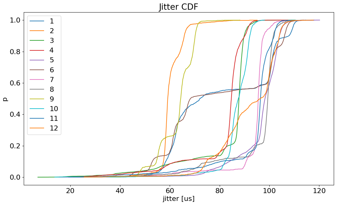
(b) Jitter CDF

Figure 26: CDF of latency and jitter of the use case network.

On the latency CDF it is still evident the presence of peaks, shown by this kind of plot by the straight lines on the upper right. Since they are rare, sparse occurrences (i.e. outliers), the probability of latencies being smaller than these values is almost 100%. However, when performing the same analysis on the time-series as featured previously, I observed that the occurrences do not have the same profile as observed on simulations from VMs.

Emission jitter also improved considerably. Where before it oscillated around 500 $\mu$s for this same configuration, the maximum observed in this simulation is 120 $\mu$s, for instance. In addition to the faster periodic execution, period overruns only start to happen with much smaller periods (< 1 ms) and heavier loads. Nonetheless, even if these values are apparently small, they can still be considered over the limit in respect to AFDX standards. Considering we do not multiplex multiple VLs into a single connection, where jitter would most likely increase due to the traffic shaping mechanism, the measured jitter can be viewed as purely technological jitter, which has a maximum admissible value of 40 $\mu$s according to the specification (see Sect. 4.5.2). Here the limitations of pure virtualization plays a part on underachieving the small jitters found on real applications.

Primarily, all the processes running periodic tasks are sharing the resources of a single machine, in contrast with the distributed nature of Integrated Modular Avionics systems—such as AFDX. An implementation making better use of multi-threading can improve greatly the jitter, but to arrive at the same level as dedicated architectures is most likely impractical.

Secondly, hard RTOSes like Xenomai guarantee the meeting of deadlines, but no assurance that it will do so as quickly as possible. This results in frames being sent much after the VL periodic release, but before the next period (too late frames, as specified on Sect. 6.2.2). Another collateral effect of this behavior is frames being dropped by the traffic policing mechanism; in the event of the succeeding frame respecting the period more strictly, the time gap between the two consecutive frame shortens, making the instant bandwidth higher than the rate configured on the token bucket algorithm.

On bigger, more complex network configurations, there are still a number of unexplained issues. Perhaps the most blatant one is the presence of negative jitters. To have negative jitter means that the periodic tasks are executing before its release point—defined by Xenomai—on the processor timeline, which is not supposed to happen. However, the existence of such jitters on data collected from simulations is most likely due to the timestamping process instead of faulty periodic behavior, which is very costly and sometimes uncertain.

7 Conclusions and Future Work

One of the main objective of this work is to evaluate the possible benefits of using formal models and virtualization technologies for the simulation of communication networks. While we concentrate on AFDX networks here, the same approach could be used with other protocols.

This work had several requirements. Some of these requirements were technical, such as developing a new virtualization framework for AFDX based on the Mininet network emulator. And some were theoretical, such as defining new formal models of AFDX networks that could precisely take into account the temporal constraints of a network. This gave me the opportunity to work with many different technologies: formal verification; networking and virtualization; programming for real-time OS; etc. which was a very rewarding experience.

During this project we developed three formal specifications for an AFDX network with different levels of approximation—(i) timed channels; (ii) direct virtual links; (iii) switched virtual links—each one increasing the precision of how frames are treated and transmitted through the network. I have also developed and enriched a network virtualization framework, integrating real-time features and implementing monitors to capture information about latency and jitter at runtime.

The framework developed with Mininet allows the virtualization of an AFDX network on a standard Linux computer, (we simply need to update the kernel in order to support the real-time capabilities added by Xenomai). This framework provides a local environment for testing network configurations, is easy to setup, and scalability mainly depends on the physical platform. While it still doesn’t have sufficient guarantees to respect the strict timing constraints, our initial benchmarks support our conviction that virtualization can be used to run simulations faster than with a real network and with an acceptable time-accuracy.

Most of the anomalies faced during development disappeared once the environment was moved out of a Virtual Machine environment. From the experiences done on a dedicated laptop it appears that the system is able to simulate an AFDX network of moderate complexity with minor drawbacks. Further work is necessary to use the system resources more efficiently in order to decrease the jitter, improve the time-stamping precision and reduce the overhead caused by the monitors, as well as using the developed benchmarking tools to better profile the virtualization performance.

An important result missing from this project is the transformation of the formal specification into runtime monitors. When porting the models described using the Fiacre language to run on the Hippo execution engine, a fundamental flaw was discovered—related to how periodicity is implemented by the engine—which hindered further development. However, the translation process demonstrated to be possible and can be easily done once the issue is resolved.

What can also be considered a major contribution of this work is the definition of a formal model for the token bucket traffic policing mechanism. When developing the virtualization framework there were limitations and particularities on existing algorithms—specifically Linux traffic control—that strayed from the behavior described on the AFDX specification. With this model we have a finer control over the mechanism operation to match exactly how it is done on a real system.

Appendix A Timed Channels

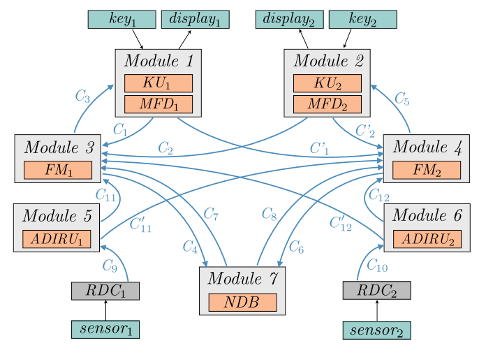
Figure 27: Use case network architecture with timed channel approximation. Source: Lauer [9]

Table 3: Timed channels parameters from the use case network

channel	source	destination	BCTT (us)	WCTT (us)
$C_{1}$	$KU_{1}$	$FM_{1}$	298	444
$C_{1}^{\prime}$	$KU_{1}$	$FM_{2}$	298	444
$C_{2}$	$KU_{2}$	$FM_{1}$	298	444
$C_{2}^{\prime}$	$KU_{2}$	$FM_{2}$	298	444
$C_{3}$	$FM_{1}$	$MFD_{1}$	310	490
$C_{4}$	$FM_{1}$	$NDB$	310	450
$C_{5}$	$FM_{2}$	$MFD_{2}$	310	490
$C_{6}$	$FM_{2}$	$NDB$	310	450
$C_{7}$	$NDB$	$FM_{1}$	400	508
$C_{8}$	$NDB$	$FM_{2}$	400	508
$C_{9}$	$RDC_{1}$	$ADIRU_{1}$	150	156
$C_{10}$	$RDC_{2}$	$ADIRU_{2}$	150	156
$C_{11}$	$ADIRU_{1}$	$FM_{1}$	452	584
$C_{11}^{\prime}$	$ADIRU_{1}$	$FM_{2}$	452	584
$C_{12}$	$ADIRU_{2}$	$FM_{2}$	452	584
$C_{12}^{\prime}$	$ADIRU_{2}$	$FM_{1}$	452	584

⬇

vlid,src,dst,bag,size

1,1,"3,4",32,75

2,2,"3,4",32,75

3,3,"1",8,625

4,3,"7",16,125

5,4,"2",8,625

6,4,"7",16,125

7,7,"3",64,500

8,7,"4",64,500

9,8,"5",32,64

10,9,"6",32,64

11,5,"3,4",32,87.5

12,6,"3,4",32,87.5

Listing 9: Use case topology described as a CSV file to be loaded by the generator.

References

- [1] Actel. Developing afdx solutions. 2005.
- [2] Alexander Beifus, Daniel Raumer, Paul Emmerich, Torsten M. Runge, Florian Wohlfart, Bernd E. Wolfinger, and Georg Carle. A study of networking software induced latency. 2015 International Conference and Workshops on Networked Systems (NetSys), 2015.
- [3] Kamal Benzekki, Abdeslam El Fergougui, and Abdelbaki Elbelrhiti Elalaoui. Software-defined networking (sdn): a survey. Security and Communication Networks, 9(18):5803–5833, 2016.
- [4] Bernard Berthomieu, Jean-Paul Bodeveix, Patrick Farail, Mamoun Filali, Hubert Garavel, Pierre Gaufillet, Frederic Lang, and François Vernadat. Fiacre: an Intermediate Language for Model Verification in the Topcased Environment. In ERTS 2008, Toulouse, France, January 2008.
- [5] Bernard Berthomieu and Francois Vernadat. Time petri nets analysis with tina. In Proceedings of the 3rd International Conference on the Quantitative Evaluation of Systems, QEST ’06, pages 123–124, Washington, DC, USA, 2006. IEEE Computer Society.
- [6] Olivier Fourcade, Patrice Thebault, Emmanuel Cloury, Stephane Gaudaire, and Bernard Mattos. Interoperability of virtual avionics equipment in aircraft development. AIAA Modeling and Simulation Technologies (MST) Conference, 2013.
- [7] Peter Heise, Fabien Geyer, and Roman Obermaisser. Deterministic openflow: Performance evaluation of sdn hardware for avionic networks. 2015 11th International Conference on Network and Service Management (CNSM), 00:372–377, 2015.
- [8] Bob Lantz, Brandon Heller, and Nick Mckeown. A network in a laptop. Proceedings of the Ninth ACM SIGCOMM Workshop on Hot Topics in Networks - Hotnets 10, 2010.
- [9] Michaël Lauer. Une méthode globale pour la vérification d’exigences temps réel : application à l’avionique modulaire intégrée. 2012.
- [10] Jean-Yves Le Boudec and Patrick Thiran. Network Calculus: A Theory of Deterministic Queuing Systems for the Internet. Springer-Verlag, Berlin, Heidelberg, 2001.
- [11] S. Martin. Maîtrise de la dimension temporelle de la qualité de service dans les réseaux. 2004.
- [12] Daniel Martinec and Samuel Buckwalter. Arinc specification 429 mark 33 digital information transfer system. Industrial Communication Technology Handbook, Second Edition Industrial Information Technology, page 1–16, 2014.
- [13] Nick Mckeown, Tom Anderson, Hari Balakrishnan, Guru Parulkar, Larry Peterson, Jennifer Rexford, Scott Shenker, and Jonathan Turner. Openflow: Enabling innovation in campus network. ACM SIGCOMM Computer Communication Review, 38(2):69, 2008.
- [14] M.j. Morgan. Integrated modular avionics for next-generation commercial airplanes. Proceedings of the IEEE 1991 National Aerospace and Electronics Conference NAECON 1991.
- [15] T. Murata. Petri nets: Properties, analysis and applications. Proceedings of the IEEE, 77(4):541–580, 1989.
- [16] Detlev Schaadt. AFDX/ARINC 664 concept, design, implementation and beyond. 2007.
- [17] Heming Wen, Prabhat Kumar Tiwary, and Tho Le-Ngoc. Network virtualization: Overview. Wireless Virtualization Springer Briefs in Computer Science, page 5–10, 2013.
- [18] M. Yao, Z. Qiu, and K. Kwak. Leaky bucket algorithms in afdx. Electronics Letters, 45(11):543, 2009.