Phenomenological theory of heat transport in the fractional quantum Hall effect

Abstract

The thermal Hall conductance is a universal and topological property which characterizes the fractional quantum Hall (FQH) state. The quantized value of the thermal Hall conductance has only recently been measured experimentally in integer quantum Hall (IQH) and FQH regimes, however, the existing setup is not able to detect if the thermal current is counter-propagating or co-propagating with the charge current. Furthermore, although there is experimental evidence for heat transfer between the edge modes and the bulk, the current theories do not take this dissipation effect in consideration. In this work we construct phenomenological rate equations for the heat currents which include equilibration processes between the edge modes and energy dissipation to an external thermal bath. Solving these equations in the limit where temperature bias is small, we compute the temperature profiles of the edge modes in a FQH state, from which we infer the two terminal thermal conductance of the state as a function of the coupling to the external bath. We show that the two terminal thermal conductance depends on the coupling strength, and can be non-universal when this coupling is very strong. Furthermore, we propose an experimental setup to examine this theory, which may also allow the determination of the sign of the thermal Hall conductance.

.1 Introduction

The fractional quantum Hall (FQH) state is a topological state of matter, and therefore it is described by universal and topological properties Prange and Girvin (1990); Wen (2007). Two such properties are the Hall conductance and the thermal Hall conductance Kane and Fisher (1995). In Abelian FQH states, which are described by an integer valued symmetric matrix, termed the $K$ matrix, these two topological properties relate to the edge modes and the $K$ matrix in different ways. The Hall conductance, given by $\sigma_{H}=\nu\frac{e^{2}}{h}$, where $\nu$ is the filling fraction, is governed by the downstream charge mode Wen (2007); Kane and Fisher (1995); Stern (2005); Kane et al. (1994). However, the thermal Hall conductance, given by

$$\kappa_{H}=n_{\text{net}}\kappa_{0}T,$$ (1)

where $\kappa_{0}=\frac{\pi^{2}k_{B}^{2}}{3h}$ is the quantum of thermal conductance Pendry (1983) and $T$ is the temperature, is governed by the net number of edge modes, $n_{\text{net}}=n_{d}-n_{u}$, which is the difference between the number of downstream and upstream modes in the edge theory Kane and Fisher (1997).

An interesting phenomenon occurs in hole-like states, which have $\frac{1}{2}<\nu<1$. Theory suggests that these states are characterized by $n_{u}\geq n_{d}$. In the case of $n_{u}>n_{d}$, when the modes are at equilibrium, charge and heat flow on different edges of the FQH liquid. Whereas, in the case of $n_{u}=n_{d}$, the heat flow is diffusive Kane and Fisher (1997); Nosiglia et al. (2018); Protopopov et al. (2017).

The thermal Hall conductance has only recently been measured in IQH states Jezouin et al. (2013); Banerjee et al. (2016), in FQH states Banerjee et al. (2016, 2018) and in the magnetic material $\alpha$-RuC$l_{3}$ Kasahara et al. (2018). However, the current setups used in these experiments cannot determine which edge carries the heat current. Hence, the thermal Hall conductance still holds more information about the $K$ matrix, which was yet realized. Furthermore, it was shown experimentally that there is energy dissipation from the edge modes of a QH state Venkatachalam et al. (2012). Energy dissipation can arise from different mechanisms. Electron-electron interaction, for example, which is accountable for the appearance of the charge and neutral modes Meir (1994); le Sueur et al. (2010); Altimiras et al. (2010); Dolev et al. (2011); Bid et al. (2011); Gross et al. (2012); Gurman et al. (2012); Wang et al. (2013); Grivnin et al. (2014); Inoue et al. (2014), may cause inter-edge-modes energy relaxation le Sueur et al. (2010); Altimiras et al. (2010), but may also account for energy loss to puddles in the bulk. Electron-phonon interaction may lead to energy dissipation from the edge modes le Sueur et al. (2010); Altimiras et al. (2012); Venkatachalam et al. (2012). Nonetheless the present theories Kane and Fisher (1997); Simon (2018); Feldman (2018); Mross et al. (2018) neglect such contribution to the heat transport of the QH state. Such energy dissipation, which may alter the thermal Hall conductance of the state, should therefore be incorporated into the theory.

In this manuscript we develop a phenomenological theory for the heat transport in the edge modes of a FQH state, which elaborates on the phenomenological equations derived in Ref. Banerjee et al. (2016), and on the theoretical analysis performed in Refs. Nosiglia et al. (2018); Protopopov et al. (2017), in order to include dissipation from the edge modes to an external thermal bath. We note that recent theoretical analysis of the observation of quantized thermal Hall conductance in the magnetic material $\alpha$-RuC$l_{3}$ Vinkler-Aviv and Rosch (2018); Ye et al. (2018), take into account coupling to phonons. However, in this three dimensional system, and in the experimental set-up employed in Ref. Kasahara et al. (2018), energy transfered to the phonons is not lost, and is included in the measured heat current. In this manuscript, and in the experiment carried out in Refs. Banerjee et al. (2016, 2018) energy transfered to phonons, or any other mode of dissipation, leaks out of the system and is not measured. By solving the heat transport rate equations for small temperature difference between the two sides of the FQH liquid, we find the temperature profiles of the edge modes, as a function of the equilibration length, $\xi_{e}$, between the modes, the dissipation length, $\xi_{d}$, for energy dissipation to the external bath, and the system size, $L$. We then define and calculate the two terminal thermal conductance, and show that its measurement may strongly depend on the dissipation length. Since we are interested in exploring the effect of dissipation on the topological thermal Hall conductance, it is required that $L\gg\xi_{e}$. While $L$ usually varies between tens to hundreds of $\mu m$, it was found experimentally that typical $\xi_{e}$ can vary between $3\mu m$ le Sueur et al. (2010) and $20\mu m$ Banerjee et al. (2016), depending on the temperature, and that $\xi_{d}$ is bounded from below by $30\mu m$ le Sueur et al. (2010). We find that for $\xi_{d}\gg\xi_{e}$ the two terminal conductance approaches the topological and universal value of Eq. (1), whereas for $\xi_{d}\ll\xi_{e}$ the two terminal thermal conductance is not universal anymore, and is sensitive to edge reconstruction processes.

Furthermore, we propose an experimental setup to test this phenomenological theory, and to determine the sign of the thermal Hall conductance. This experimental setup relies on quantum dots (QDs) which are coupled to the edges of a FQH state. By exploiting a relation between the thermoelectric coefficient and the electric conductance of the QDs Roura-Bas et al. (2018), we point out that they can be used as local thermometers for electrons on the FQH edge state. The local temperatures of the edge states can be deduced from a measurement of the thermoelectric current through the QDs, and thus the temperature profiles can be measured. We show that the sign of the thermal Hall conductance may be determined from the measured temperature profiles.

.2 Phenomenological heat transport theory in Abelian FQH states

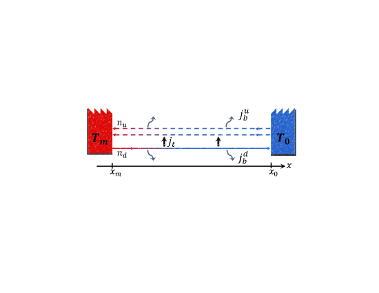
Figure 1: An illustration of the lower edge of a FQH liquid in a two terminal system, with $n_{d}$ downstream modes (solid lines) and $n_{u}$ upstream mode (dashed lines), propagating in the opposite direction. Temperature difference is applied between the right and left contacts, $\Delta T=T_{m}-T_{0}>0$. The black vertical arrows represent the equilibration current density between the edge modes on the same edge. The blue wiggly arrows represent the dissipation current density, to the external thermal bath.

Without loss of generality, we assume the directions of flow of the edge modes on the lower edge of a FQH state are as depicted in Fig. (1). On the upper edge $n_{u}\leftrightarrow n_{d}$ and the directions of flow of the edge modes are reversed. In this situation the FQH state has $n_{d}$ downstream modes and $n_{u}$ upstream modes, which for this analysis are assumed to obey $n_{d}\neq n_{u}$. We shall consider the case $n_{u}=n_{d}=1$ when we discuss the $\nu=\frac{2}{3}$ FQH state. The downstream modes on the lower edge are emanating from an Ohmic contact at position $x_{m}$ at temperature $T_{m}$, and the upstream modes are emanating from another Ohmic contact at position $x_{0}$ at temperature $T_{0}$. Both Ohmic contacts are at the same chemical potential. For $T_{m}>T_{0}$, the downstream modes are expected to be hotter than the upstream modes. Thus energy will be transferred from the downstream to the upstream modes, through a heat current density $j_{t}$, in order to achieve equilibration. In addition, in order to model dissipation, we assume the edge modes are coupled to an external thermal bath kept at temperature $T_{0}$, such that there are dissipation current densities $j_{b}^{d}$ and $j_{b}^{u}$ from the downstream and upstream modes to the bath. Assuming that energy is conserved in the system composed of the edge modes and the external bath, the heat currents flowing through the 1D downstream modes and the 1D upstream modes, denoted by $J_{d}$ and $J_{u}$ respectively, are described by the following rate equations:

$$J_{d}\left(x+\delta x\right) =J_{d}\left(x\right)-j_{t}\left(x\right)\delta x-j_{b}^{d}\left(x\right)\delta x$$ (2)

$$J_{u}\left(x\right) =J_{u}\left(x+\delta x\right)+j_{t}\left(x\right)\delta x-j_{b}^{u}\left(x\right)\delta x.$$

Temperature profiles

The temperature dependencies of the heat currents in Eq. (2) are modeled as follows. The heat current flowing in the 1D downstream and upstream edge modes is modeled as $J_{i}(x)=\frac{1}{2}\kappa_{0}n_{i}T_{i}^{2}(x)$ Kane and Fisher (1997), where $i=d,u$. The equilibration current density $j_{t}$ is modeled by Newton’s law of cooling, $j_{t}\left(x\right)=\frac{1}{2}\frac{\kappa_{0}}{\xi_{e}}\left[T_{d}^{2}\left(x\right)-T_{u}^{2}\left(x\right)\right]$, where $\xi_{e}$ is the relaxation length, similarly to Ref. Banerjee et al. (2016). The dissipation current to the external thermal bath is modeled by a temperature power law relative to the bath temperature: $j_{b}^{i}(x)=\frac{1}{2}\kappa_{0}n_{i}B(T_{i}^{\alpha}(x)-T_{0}^{\alpha})$. The exponent $\alpha$ has different values depending on the mechanism of dissipation. Energy transfer from electron to phonons, for example, may lead to $\alpha=5$, but also to smaller values depending on details C. Wellstood et al. (1994). Electron-electron interaction gives $1<\alpha<2$, depending on the extent to which impurities are involved Imry (2002). To simplify the solution and further treatment, we write the equations using the dimensionless parameter: $\tau_{i}\left(x\right)=\frac{T_{i}^{2}\left(x\right)}{T_{0}^{2}}$, and we denote: $\beta=BT_{0}^{\alpha-2}$. Then, the equations can be written as a set of coupled differential equations for $\tau_{u}$ and $\tau_{d}$:

$$\frac{d\tau_{d}}{dx} =-\frac{1}{n_{d}\xi_{e}}\left(\tau_{d}\left(x\right)-\tau_{u}\left(x\right)\right)-\beta\left(\tau_{d}^{\frac{\alpha}{2}}\left(x\right)-1\right)$$ (3)

$$\frac{d\tau_{u}}{dx} =-\frac{1}{n_{u}\xi_{e}}\left(\tau_{d}\left(x\right)-\tau_{u}\left(x\right)\right)+\beta\left(\tau_{u}^{\frac{\alpha}{2}}\left(x\right)-1\right).$$

The temperature dependence of the heat currents to the thermal bath and the exchange current are expected to hold for small temperature difference, $\Delta T=T_{m}-T_{0}$. The boundary conditions are:

$$\tau_{d}\left(x_{m}\right)=\tau_{m}=\frac{T_{m}^{2}}{T_{0}^{2}} \quad;\quad \tau_{u}\left(x_{0}\right)=1=\frac{T_{0}^{2}}{T_{0}^{2}}.$$ (4)

An analytic solution to Eqs. (3), with the boundary conditions given by Eq. (4) can be obtained for small temperature difference from $T_{0}$, i.e. $\Delta T\ll T_{0}$, such that $\tau_{i}\left(x\right)=1+\delta\tau_{i}\left(x\right)$. Linearizing the equations, we find a new interaction parameter, $\frac{1}{\xi_{d}}=\frac{\beta\alpha}{2}$, which we call the dissipation length. Integrating the linearized differential equations with the appropriate boundary conditions, $\tau_{d}\left(x\right)$ and $\tau_{u}\left(x\right)$ of the lower edge are obtained:

$$\tau_{d}^{\text{lower}}\left(x\right) =1+\frac{\left(\frac{N}{2\bar{n}}+\frac{\xi_{e}}{\xi_{d}}\right)\sinh\left[\Lambda\left(x_{0}-x\right)\right]+\Lambda\xi_{e}\cosh\left[\Lambda\left(x_{0}-x\right)\right]}{\left(\frac{N}{2\bar{n}}+\frac{\xi_{e}}{\xi_{d}}\right)\sinh\left[\Lambda L\right]+\Lambda\xi_{e}\cosh\left[\Lambda L\right]}e^{-\frac{x-x_{m}}{2\bar{n}\xi_{e}}}\left(\tau_{m}-1\right)$$ (5a)

$$\tau_{u}^{\text{lower}}\left(x\right) =1+\frac{1}{n_{u}}\frac{\sinh\left[\Lambda\left(x_{0}-x\right)\right]}{\left(\frac{N}{2\bar{n}}+\frac{\xi_{e}}{\xi_{d}}\right)\sinh\left[\Lambda L\right]+\Lambda\xi_{e}\cosh\left[\Lambda L\right]}e^{-\frac{x-x_{m}}{2\bar{n}\xi_{e}}}\left(\tau_{m}-1\right),$$ (5b)

where $L=x_{0}-x_{m}$, $\bar{n}=\frac{n_{u}n_{d}}{n_{u}-n_{d}}$, $N=\frac{n_{u}+n_{d}}{n_{u}-n_{d}}$ and $\Lambda=\frac{1}{2\bar{n}\xi_{e}}\sqrt{1+4\bar{n}^{2}\frac{\xi_{e}}{\xi_{d}}\left(\frac{N}{\bar{n}}+\frac{\xi_{e}}{\xi_{d}}\right)}$. To determine $\tau_{d/u}\left(x\right)$ on the upper edge, the number of edge modes needs to be interchanged, $n_{u}\leftrightarrow n_{d}$, and for consistency with the direction of chirality also $\tau_{d}\leftrightarrow\tau_{u}$, such that $\tau_{d}^{\text{lower}}\left(x;n_{d},n_{u}\right)=\tau_{u}^{\text{upper}}\left(x;n_{u},n_{d}\right)$. Numerically we can go beyond the linearized regime, however in doing so we found that small deviations from that regime do not change the qualitative picture.

Normalized two terminal thermal conductance

Assuming that heat can be transported from the hot contact to the system only through the edge modes, the normalized two terminal thermal conductance, $\kappa$, is defined according to:

$$J_{Q}=\frac{1}{2}\kappa_{0}\kappa\left(T_{m}^{2}-T_{0}^{2}\right),$$ (6)

where $J_{Q}$ is the total heat current emanating from the hot contact to the system, due to $\Delta T$. This $\kappa$ is composed of two parts, corresponding to the heat flowing along the upper and lower edges, which by assumption do not interact. Due to energy conservation, the sum of the heat flowing in the edge modes and the integrated heat dissipated to the thermal bath should not depend on the position along the edge. Therefore, the contribution of the lower edge to the two terminal thermal conductance is:

$$\kappa_{\text{lower}}=\frac{J_{d}\left(x\right)-J_{u}\left(x\right)-J_{p}+\intop_{x_{m}}^{x}\left[j_{b}^{d}\left(x^{\prime}\right)+j_{b}^{u}\left(x^{\prime}\right)\right]dx^{\prime}}{\frac{1}{2}\kappa_{0}\left(T_{m}^{2}-T_{0}^{2}\right)},$$ (7)

where $J_{p}=\frac{1}{2}\kappa_{0}\left(n_{d}-n_{u}\right)T_{0}^{2}$ is the persistent heat current in the system at equilibrium, which has no divergence because the upper edge has an opposite term. It is subtracted from both edges in order to expose the net current above the equilibrium current flowing in the system due to the chirality.

The normalized two terminal thermal conductance of the system is obtained by summing the contributions from both edges. Plugging the temperature dependencies, given by Eqs. (5a) and (5b), the two terminal thermal conductance is readily obtained:

$$\kappa\left(\xi_{d},\xi_{e},L\right)=\kappa_{\text{lower}}+\kappa_{\text{upper}}=\frac{1}{2\bar{n}}\frac{n_{u}e^{\Lambda L}+n_{d}e^{-\Lambda L}}{\Lambda\xi_{e}\cosh\left(\Lambda L\right)+\left(\frac{N}{2\bar{n}}+\frac{\xi_{e}}{\xi_{d}}\right)\sinh\left(\Lambda L\right)}+\left(n_{u}+n_{d}\right)\frac{\left(\Lambda\xi_{e}-\frac{1}{2\bar{n}}\right)\cosh\left(\Lambda L\right)+\frac{\xi_{e}}{\xi_{d}}\sinh\left(\Lambda L\right)}{\Lambda\xi_{e}\cosh\left(\Lambda L\right)+\left(\frac{N}{2\bar{n}}+\frac{\xi_{e}}{\xi_{d}}\right)\sinh\left(\Lambda L\right)}.$$ (8)

There are three competing length scales in our problem: the system size $L$, the equilibration length $\xi_{e}$, and the dissipation length $\xi_{d}$. Since we wish to discuss the thermal Hall conductance, defined for a fully equilibrated edge system, it is required that $L\gg\xi_{e}$, so that the edge modes are able to equilibrate over the length of the system. Let us now elaborate more on the temperature profiles and $\kappa$ of the hole like states, for both cases: (i) $n_{u}>n_{d}$ and (ii) $n_{d}=n_{u}=1$ (corresponding to the $\nu=\frac{2}{3}$ state).

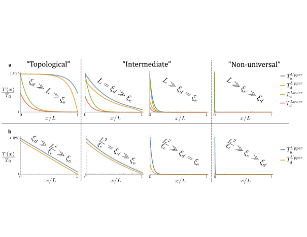
Figure 2: a. Temperature profiles of the downstream and upstream modes on the upper and lower edges of a $\nu=\frac{3}{5}$ FQH state, described by $n_{d}=1$ and $n_{u}=2$. The temperature profiles are plotted for different values of $\xi_{d}$ relative to $L$ and $\xi_{e}$, where $L=300\mu m$ and $\xi_{e}=20\mu m$ Banerjee et al. (2016). b. Temperature profiles of the downstream and upstream modes of a $\nu=\frac{2}{3}$ FQH state, described by $n_{d}=n_{u}=1$. The upper and lower edges exhibit the same temperature profile.

Hole-like states with $n_{u}>n_{d}$ -

The temperature profiles of the edge modes are given by Eqs (5a) and (5b), and $\kappa$ is given by Eq. 8. To illuminate the physics let us discuss the temperature profiles [Fig. (2.a)] and $\kappa$ in the following regimes:

Topological regime ($\xi_{d}\gg L\gg\xi_{e}$) - The edge modes exchange energy with one another, and equilibrate to the temperature of the upstream modes. In this regime their dissipation of energy to the thermal bath is small. The normalized two terminal thermal conductance acquires the absolute value of the topological value Kane and Fisher (1997) with two corrections to leading orders: $\kappa=\left(n_{u}-n_{d}\right)\left[1+2\frac{n_{d}}{n_{u}}e^{-\frac{L}{\bar{n}\xi_{e}}}\right]+4\bar{n}n_{d}\frac{\xi_{e}}{\xi_{d}}$. The first exponential correction is due to the finite system size $L$, and the second algebraic correction is due to dissipation to the bath, that happens all along the edge.

Intermediate regime ($L\gg\xi_{d}\gg\xi_{e}$) - Most energy is dissipated to the thermal bath before arrival to the cold contact, therefore the temperature profiles decrease to $T_{0}$ on both edges. However, the edge modes exchange energy before dissipating it all to the thermal bath. Thus, to leading order, $\kappa$ acquires the absolute value of the topological value, with an algebraic correction due to dissipation: $\kappa=\left(n_{u}-n_{d}\right)+4\bar{n}n_{d}\frac{\xi_{e}}{\xi_{d}}$. This correction can be of the order of $\left(n_{u}-n_{d}\right)$, so $\kappa$ is not universal in this case.

Non-universal regime ($L\gg\xi_{e}\gg\xi_{d}$) - The edge modes dissipate all their energy to the thermal bath and therefore the temperature profiles decrease to $T_{0}$ very close to the hot contact. The thermal conductance, $\kappa$, in this case is the total number of edge modes leaving the hot contact, $n=n_{u}+n_{d}$, with a correction due to a competition between $\xi_{e}$ and $\xi_{d}$: $\kappa=\left(n_{u}+n_{d}\right)-\frac{\xi_{d}}{\xi_{e}}$. This happens because the modes emanating from the hot contact on both edges dissipate all the energy to the external thermal bath, thus the heat conductance is limited by the total number of modes emanating the hot contact. The number $n=n_{u}+n_{d}$ is not universal, due to processes such as edge reconstruction Wan et al. (2003); Sabo et al. (2017). This limit and the limit of a very short system, i.e. $L\ll\xi_{e}$, are qualitatively similar.

$\nu=\frac{2}{3}$ state -

The temperature profiles of the edge modes of the $\nu=\frac{2}{3}$ state are obtained by taking the limit of $n_{u}\rightarrow n_{d}=1$ in Eqs. (5a), (5b). Substituting the temperature profiles into Eq. 7 we obtain $\kappa$ for the $\nu=\frac{2}{3}$ state:

$$\kappa=2\left[1-\frac{1}{1+\frac{\xi_{e}}{\xi_{d}}+\Lambda_{\frac{2}{3}}\xi_{e}\coth\left(\Lambda_{\frac{2}{3}}L\right)}\right],$$ (9)

where $\Lambda_{\frac{2}{3}}=\frac{1}{\xi_{e}}\sqrt{\frac{\xi_{e}}{\xi_{d}}\left(2+\frac{\xi_{e}}{\xi_{d}}\right)}$. To illuminate the physics, let us discuss the temperature profiles of the edge modes [Fig. (2.b)] and $\kappa$ in the corresponding three regimes:

The topological regime ($\xi_{d}\gg\nicefrac{{L^{2}}}{{\xi_{e}}}\gg\xi_{e}$) - The system is diffusive, therefore the temperature profiles are linear along the edges, with a constant difference. The thermal conductance, $\kappa$, approaches the absolute value of the topological value Kane and Fisher (1997) with a leading order algebraic correction, due to a competition between the equilibration length and the finite system size: $\kappa=\frac{2}{1+\frac{L}{\xi_{e}}}$.

The intermediate regime ($\nicefrac{{L^{2}}}{{\xi_{e}}}\gg\xi_{d}\gg\xi_{e}$) - The system dissipate energy to the thermal bath, therefore the temperature profiles are exponential, rather than linear. The thermal conductance, $\kappa$, approaches the absolute value of the topological value, with a leading order algebraic correction, due to the competition between the equilibration and dissipation lengths: $\kappa=\frac{2}{1+\sqrt{2\frac{\xi_{d}}{\xi_{e}}}}$.

The non-universal regime ($\nicefrac{{L^{2}}}{{\xi_{e}}}\gg\xi_{e}\gg\xi_{d}$) - The edge modes dissipate all their energy to the thermal bath, so the temperature profiles decrease to $T_{0}$ very close to the hot contact. The thermal conductance, $\kappa$, approaches the non-universal value of the total number of modes, with an algebraic correction due to the competition between equilibration and dissipation: $\kappa=2-\frac{\xi_{d}}{\xi_{e}}$.

.3 Proposed experimental setup

This phenomenological theory may be tested by employing quantum dots (QDs) as thermometers Hoffmann et al. (2007); Venkatachalam et al. (2012); Viola et al. (2012); Maradan et al. (2014) for the temperature at various points along the edge. The proposed experimental setup, depicted in Fig. (3), couples QDs to the edges of FQH liquids, and is based on measuring the resulting thermoelectric current. To deduce the temperature profiles from the thermoelectric current, the thermoelectric coefficient needs to be known. Following Furusaki Furusaki (1998), the thermoelectric coefficient, $G_{T},$ of a QD in a normal state, weakly coupled to two FQH liquids, can be calculated to linear order in the temperature difference between the two FQH states. In this regime, the thermoelectric coefficient is found to be related to the conductance of the QD Roura-Bas et al. (2018) as

$$G_{T}=\frac{\epsilon}{e}G,$$ (10)

where $G$ is the linear electric conductance of the QD, $e$ is the electron charge and $\epsilon$ is the energy difference between the many body ground state energies of $N+1$ electrons and $N$ electrons in the QD. Using this relation, the thermoelectric coefficient of the QDs can be measured without applying a temperature bias. Thus the temperature profiles can be deduced from the thermoelectric current through the QDs, upon introduction of temperature difference $\Delta T$.

A measurement of the temperature profiles allows for the extraction of the dissipation length, the equilibration length and the sign of the thermal Hall conductance. For extraction of the latter, the system needs to be in the topological regime ($\xi_{d}\gg L\gg\xi_{e}$). In this regime, the edges are distinguished by their temperature profiles, such that the edge which is expected to carry the heat current, according to Ref. Kane and Fisher (1997) is hotter [Fig. (2)].

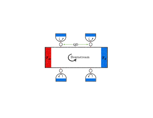
Figure 3: A schematic picture of the proposed experimental setup. Two Ohmic contacts are connected to a Hall bar at a FQH state, with a chirality defined by the solid black arrow. A temperature difference $\Delta T=T_{m}-T_{0}$ is imposed between the contacts (Ref. Banerjee et al. (2016); Jezouin et al. (2013)). Multiple number of QDs, depicted by the full circles, are coupled to both edges of the Hall bar. They are connected to Ohmic contacts, thus enabling measurement of the thermoelectric currents that passes through them.

.4 Conclusions

To conclude, the thermal Hall conductance is predicted to be a universal and topological property of a FQH state, and therefore can help determining the states in a more accurate way. Recent experiment has managed to measure the absolute value of the thermal Hall conductance of Abelian FQH states Banerjee et al. (2016), and consisted with the prediction of Kane and Fisher Kane and Fisher (1997) regarding these states. It should be noted, however, that Ref Kane and Fisher (1997) assumes the edge is a closed system with respect to energy, while it was shown experimentally that there can be energy dissipation from the edge Venkatachalam et al. (2012).

In this paper we elaborated on the phenomenological picture of the temperature profiles of the edge modes of a FQH state with $n_{d}$ downstream mode and $n_{u}$ upstream modes described in Ref. Banerjee et al. (2016), by writing rate equations for heat transport through the edges, including a dissipation term to an external thermal bath. By solving the phenomenological equations, we found that the two terminal thermal conductance depends on the coupling strength to the external thermal bath, in such a way that when the coupling is extremely weak, the two terminal thermal conductance acquires the universal topological value, however, when the coupling is very strong the two terminal thermal conductance is not universal anymore, and is subject to the influence of edge reconstruction effects Wan et al. (2003); Sabo et al. (2017).

Furthermore, we proposed to use QDs coupled to the edges of a FQH state to, first, test the above theory and measure the dissipation length and the equilibration length, and second, to determine the sign of the thermal Hall conductance.