Quantum limited superresolution of an incoherent source pair in three dimensions
Abstract
The error in estimating the separation of a pair of incoherent sources from radiation emitted by them and subsequently captured by an imager is fundamentally bounded below by the inverse of the corresponding quantum Fisher information (QFI) matrix. We calculate the QFI for estimating the full three-dimensional (3D) pair separation vector, extending previous work on pair separation in one and two dimensions. We also show that the pair-separation QFI is, in fact, identical to source localization QFI, which underscores the fundamental importance of photon-state localization in determining the ultimate estimation-theoretic bound for both problems. We also propose general coherent-projection bases that can attain the QFI in two special cases. We present simulations of an approximate experimental realization of such quantum limited pair superresolution using the Zernike basis, confirming the achievability of the QFI bounds.
pacs:
(100.6640) Superresolution; (110.3055) Information theoretical analysis; (110.6880) Three-dimensional image acquisition; (110.7348) Wavefront encoding; (110.1758) Computational imaging; (270.5585) Quantum information and processingRayleigh’s pair-resolution criterionRayleigh is routinely superseded by modern imaging systems. An approach that entirely circumvents it employs PSF fitting and localization of single fluorescent molecules by selective excitation in which two closeby molecules are rarely, if ever, excited simultaneously Moerner89 ; Hell94 ; Betzig95 in each frame, thus allowing a frame-by-frame construction of a composite, superresolved image of a collection of densely packed molecules. Another, more direct approach uses computational image processing with a priori constraints under sufficiently high pixel brightness RH68 ; BdM96 ; Lucy92 ; SM04 ; RWO06 ; Prasad14 .
The covariance matrix, , for the unbiased estimator, , of a set of quantities, , parameterizing the density operator, , of a system is bounded below by the inverse of the quantum Fisher information (QFI) matrix Helstrom76 ; Braunstein94 ; Paris09 ; Szczykulska16 ; Safranek18 , namely the quantum Cramér-Rao bound (QCRB),
| (1) |
in which defines a positive-operator valued measure (POVM) of non-negative operators defined on a data set and which sum to the identity operator, . The classical FI matrix, , is defined VT68 ; Kay93 in terms of the probability distribution (PD) of the POVM, , as
| (2) |
in which is a column vector representing the gradient taken relative to , the superscript denotes matrix transpose, and the statistical expectation of its argument over the PD. The inverse of the classical FI is the classical Cramér-Rao lower bound (CRB).
Tsang et al. Tsang16 proved that pair separation can achieve QCRB in one dimension with classical wavefront projections. This has been generalized to a thermal source pair of the same average but otherwise indefinite strength Nair16 , to a source pair in an arbitrary quantum state Lupo16 , to homodyne and heterodyne detectionYang17 , and to two dimensions Ang17 , and experimentally verified by a number of groups Paur16 ; Tang16 ; Yang16 ; Tham17 . For an imager with a one dimensional (1D) Gaussian point-spread function (PSF), it is the Hermite Gaussian (HG) basis Tsang16 that perfectly achieves QCRB, which turns out to be independent of the pair separation. By contrast, the conventional image-based approach entails a quadratic dependence of FI on the separation. This critical difference implies dramatically different inverse-square vs. inverse-quartic power-law scalings of the minimum photon number needed to resolve the pair as a function of their separation using these two approaches.
Here we treat the problem of estimating the full 3D separation vector for a pair of incoherent, equally bright point sources, when the pair centroid is known and an imager with a circular aperture is used PrasadYu17 . We first calculate the QFI matrix with respect to (w.r.t.) the three components of the pair separation vector, and show it to be diagonal and independent of the latter. We also show that QFI is in fact the same as that for localizing a single point emitter in 3D Backlund18 . We then discuss projective-measurement protocols that can achieve QCRB in two special cases of vanishing axial and lateral separations. We finally present simulations of an experimental proposal to achieve quantum-limited 3D pair separation.
A photon emitted by an incoherent pair of equally bright point sources is described by the density operator,
| (3) |
in which are pure one-photon states corresponding to its emission individually by the two sources taken to be at the 3D locations, , with respect to their centroid. The corresponding normalized transverse and axial semi-separations, , are defined as
| (4) |
where and denote the characteristic transverse and axial resolution scales for an aperture of radius , optical wavelength , and distance of the pair centroid from the apertureGoodman17 .
The coordinate representations, , of these states are the corresponding image-plane amplitude PSFs. Their momentum-space representations are the corresponding wavefunctions in the exit pupil of the imager Goodman17 ,
| (5) |
in which denoted a general aperture function. For a clear aperture, is simply times its indicator function, corresponding to the Airy PSF, while in its Gaussian form, it yields the Gaussian PSF. Most generally, need only obey the normalization condition,
| (6) |
that follows from requiring .
The two non-zero eigenvalues, , and the associated orthonormal eigenstates, , of given by Eq. (3) are
| (7) |
where is the inner product, which we render real and positive by a proper choice of the phase constant, .
The QFI matrix has elements, , where Re denotes the real part and can be expressed supp in the eigenbasis of as
| (8) |
in which is the symmetric logarithmic derivative (SLD) of w.r.t. parameter , for brevity we denote as , and denotes the set of values of an index for the eigenstates that span the range space of .
By decomposing the sum into a sum over the range space of and another over its null space, for which , we may evaluate the latter sum via the completeness relation,
We may thus express in Eq. (8) as
| (9) |
For the present problem for which , we may simplify the derivatives in Eq. (Quantum limited superresolution of an incoherent source pair in three dimensions) by means of the eigenvector identity, and thus express as supp
| (10) |
in which we used the identities, and . The first sum in expression (Quantum limited superresolution of an incoherent source pair in three dimensions) may be regarded as the classical part of QFI, the real part of the second sum the contribution of quantum fluctuations of the photon state to QFI, and the real part of the final sum an additional contribution from the pair cross-coherence, .
By evaluating the various state derivatives in expression (Quantum limited superresolution of an incoherent source pair in three dimensions), we may reduce it further supp to the form,
| (11) |
By using expression (5) for , we may evaluate Eq. (11) in terms of the gradient of the phase function,
| (12) |
independently of as
| (13) |
where angular brackets now denote averages over the modulus squared aperture function, .
Form (13) of QFI underscores the fundamental role of the correlations of the wavefront gradient in the aperture in controlling the error of estimation of the pair separation. For a clear circular aperture, to which we restrict attention in the rest of the paper and for which is times its indicator function, simple integrations yield the following averages:
| (14) |
and thus the following purely diagonal form of the per-photon 3D QFI matrix:
| (15) |
The reality and diagonal character of provide necessary and sufficient achievability conditions for the simultaneous estimation of the three separation coordinates in the asymptotic limit Ragy16 .
We next show that QFI for localizing a single source, say the one located at , is identical to that we have just obtained for 3D pair separation. For this problem, only the middle term in expression (Quantum limited superresolution of an incoherent source pair in three dimensions) contributes, since has a single fixed non-zero eigenvalue, , with eigenstate , and . In view of these relations and normalization, , which requires that , the resulting QFI becomes identical to Eq. (11) for QFI for source-pair separation. The 3D source-localization QFI has been calculated directly from the definition of SLD of the density opermator for a pure state in Ref. Backlund18 , but unlike that approach ours can be more efficiently extended, numerically if necessary, to calculate QFI for joint source localization and separation of two or more sources emitting single photons in a general state PrasadYu18 . The equality of the QFI matrices for source localization and pair separation shows that the general problem is one of estimating the photon state, independent of the nature of its emitter.
QCRB is achievable via orthonormal wavefront projections in two special cases. For sources in the same transverse plane, for which , consider an orthonormal basis, , of states in the aperture plane obeying the condition, . Since , this condition is met by any real basis. The probability , which is equal to , may then be written as from which follow the FI matrix elements,
| (16) |
If we assume further that the phases of are independent of , then Eq. (Quantum limited superresolution of an incoherent source pair in three dimensions) simplifies to
| (17) |
with the second equality following from the completeness relation, . For , matches QFI in expression (11) since for the choice, , we make to render the phases of independent of , , vanishes identically for any inversion symmetric aperture.
The orthonormal sine-cosine Fourier basis states in polar coordinates, ,
| (18) |
with , constitute one such basis that achieves QFI for the case of pure transverse pair separation as their overlap integrals with the photon wavefront of each source can be readily shown supp to have phases that are independent of that separation.
For the source pair being on the optical axis, i.e., , only the subset of the sine-cosine basis, as we need no angular localization, achieves QCRB w.r.t. , as we show next. The relevant probability amplitudes are
| (19) |
with . We used the variable transformation, , followed by a symmetrization of the resulting integrand to reach the second equality in Eq. (Quantum limited superresolution of an incoherent source pair in three dimensions) that involves a purely real integral. In view of the form (Quantum limited superresolution of an incoherent source pair in three dimensions), we have , which allows us, analogously to Eq. (Quantum limited superresolution of an incoherent source pair in three dimensions) with , to express FI w.r.t. as
| (20) |
in which we used the completeness of the states over the aperture for -invariant wavefunctions like characteristic of an axially separated source pair and relations, , to derive the various expressions. We see from expression (11) that the basis achieves QFI w.r.t. for an axially separated source pair. More generally, any real basis of orthonormal projections, , for which the equality, , certainly holds, will achieve QFI.
Projections that are well matched to the linear tilt and quadratic defocus parts of the aperture phase function, , given by Eq. (12), can achieve full 3D QFI in the limit of small separations, . One need merely use a few such projections, as noted in Ref. Tsang16 ), to attain quantum-limited estimation variance in this limit. In the 3D case, we consider aperture-plane wavefront projections into low-order orthonormal Zernike basis functions Noll76 , , with . Here we only discuss projections into the first four Zernikes,
| (21) |
The second and third of these correlate perfectly, respectively, with the tilt phases corresponding to the and components of the transverse separation vector, , and may thus be regarded as matched filters Turin60 for the latter. By contrast, the first and last are only partially matched to the quadratic pupil phase corresponding to the axial separation, , with their probabilities remaining finite when . The imperfect match of the latter with a single projection mode causes striking differences, as we shall see, in the estimation error bounds that are achievable in the limit of vanishing separation.
We now prove these assertions by evaluating supp the mode-projection probabilities, , for ,
| (22) |
Since , we see that each reaches QFI in the limit . By contrast, the projection contributes to FI w.r.t. the term, , which is of form and vanishes in the limit if . The same form implies, however, that for , FI as a function of rises to a value comparable to the QFI, , over an interval of order . All other contributions to the various matrix elements of FI are negligibly small in the limit of vanishing , so the inverse of the diagonal elements of FI determine the corresponding CRBs to the most significant order in .
One can perform wavefront projections by digital holography Paur16 . Specifically, consider encoding the sum, , as the distribution of the amplitude transmittance of a plate, with negative values in the sum realized by a phase retardation. Let the imaging wavefront, which is an incoherent superposition of the photon wavefunctions and carries photons, be incident on such a plate that is placed in the aperture (or a conjugate plane thereof), and then optically focused on a sensor. The photons will divide into pairs of oppositely located spots, with the th pair of spots corresponding to an obliquely propagating wave pair that carries the projection of the incident wavefront along the spherical-angle pair, , with . The numbers of photons detected at the central pixels of the spots taken pairwise furnish estimates of the probabilities of the wavefront being in the corresponding modes. The remaining photons that are not detected provide an estimate of the wavefront being in the remaining states of a complete basis of which the subset, defines the observed states. The probability of detecting photons in the projective channels is given by the multinomial (MN) distribution supp ,
| (23) |
in which and are, respectively, the number and probability of undetected photons. Expressing the in terms of the separation coordinates, , we performed their maximum-likelihood (ML) estimation by numerically minimizing over those coordinates using Matlab’s fminunc minimizer, which we started with an initial guess of , for a number of separations, 20,000 frames of noisy data, each with photons and generated using Matlab’s mnrnd code.
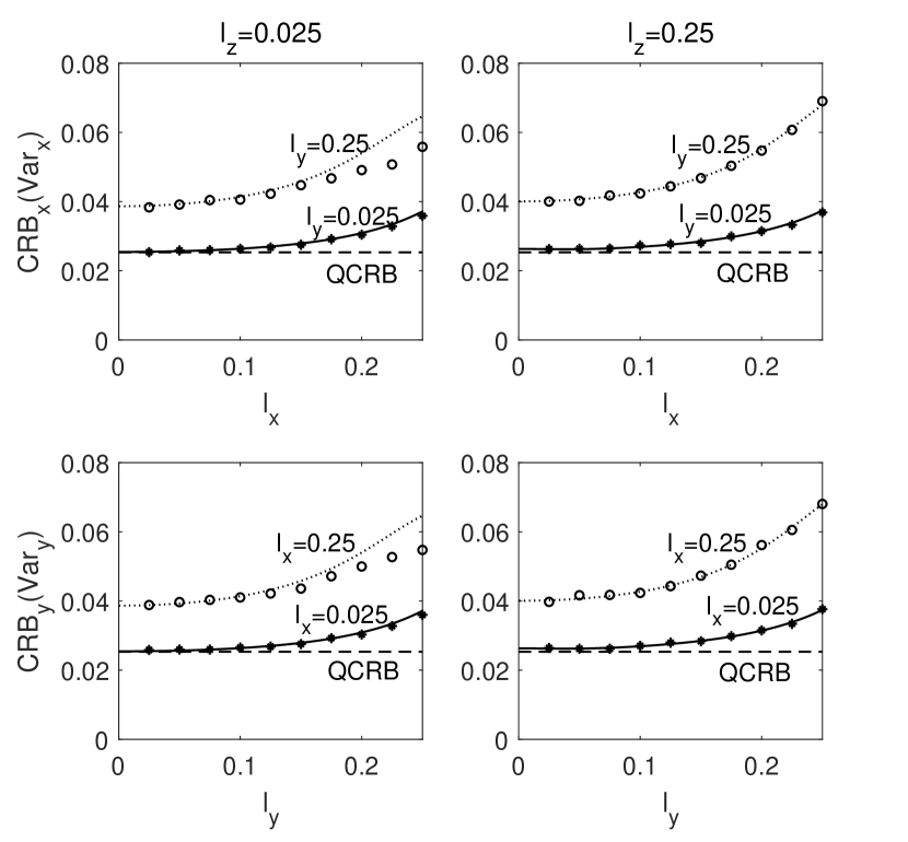
We plot in Fig. 1 the per-photon CRBs w.r.t. (top panels) and (bottom panels) for two different values of their axial separation, (left panels) and 0.25 (right panels). For each plot, we considered two different values, 0.025 and 0.25, of the other transverse coordinate, shown via the two different curves in each figure. Note that CRB w.r.t. each transverse-separation coordinate increases with increasing value of the other coordinate due to a cross-talk between the two transverse coordinates. Changing the longitudinal separation, however, has a less pronounced effect on those curves. As the pair separation increases, using only the first four Zernikes is insufficient to estimate , which accounts in part for the rising CRB curves.The discrete points identified by marker symbols are the results of the sample-based variance (per photon) of the ML estimate of the separation coordinates that we obtained in our numerical simulations. Note that the results of simulation are consistently lower than the corresponding CRB curves, which is most discernible in the left panels (). This is because the ML estimates of the separation coordinates are biased, particularly that for , and standard CRBs do not provide the correct lower bounds without including bias-gradient based modifications VT68 ; Kay93 .
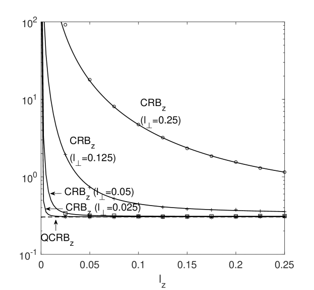
In Fig. 2 we plot the per-photon CRBs w.r.t. for four different values of . We observe divergent behavior as approaches zero, corresponding to the vanishing of whenver that we noted earlier. This behavior is quite in contrast with the rather muted dependence on which we observed in Fig. 1 for the CRBs w.r.t. . The cross-talk between the uncertainties in simultaneously estimating the three pair-separation coordinates inherently present in the small set of Zernike projections increases the CRB for estimation as increases. The simulated values of the variance for estimating , indicated by marker symbols, agree well with the theoretical CRB values, with evidence of any bias only for .
This Letter has treated the fundamental error in estimating the full 3D separation vector for a source pair by calculating the corresponding QFI and proposing specific projection bases for which QFI is attainable. Simulations using the Zernike basis confirm our theoretical assertions.
Acknowledgments
The work was partially supported by the US Air Force Office of Scientific Research under grant no. FA9550-15-1-0286. The authors are grateful to G. Adesso for pointing out his group’s very recent work Napoli18 on the simultaneous estimation of the angular and axial separations as well as the coordinates of the centroid of an incoherent source pair located in a single meridional plane.
References
- (1) L. Rayleigh, “XXXI. Investigations in Optics, with Special Reference to the Spectroscope,” Philos. Mag. 8, 261 (1879).
- (2) W. E. Moerner and L. Kador, “Optical detection and spectroscopy of single molecules in a solid,” Phys. Rev. Lett. 62, 2535 (1989).
- (3) S. W. Hell and J. Wichmann, “Breaking the diffraction resolution limit by stimulated emission: stimulated-emission-depletion fluorescence microscopy,” Opt. Lett. 19, 780 (1994).
- (4) E. Betzig, “Proposed method for molecular optical imaging,” Opt. Lett. 20, 237 (1995).
- (5) C. Rushforth and R. Harris, “Restoration, resolution, and noise,” J. Opt. Soc. Am. 58, 539-545 (1968).
- (6) M. Bertero and C. De Mol, “Superresolution by data inversion,” Progress in Optics XXXVI, 129-178 (1996).
- (7) L. Lucy, “Statistical limits to superresolution,” Astron. Astrophys. 261, 706-710 (1992).
- (8) M. Shahram and P. Milanfar, “Imaging below the diffraction limit: a statistical analysis,” IEEE Trans. Image Process. 13, 677-689 (2004).
- (9) S. Ram, E. Sally Ward, and R. Ober, “Beyond Rayleigh’s criterion: a resolution measure with application to single-molecule microscopy,” Proc. Natl. Acad. Sci. USA 103, 4457-4462 (2006).
- (10) S. Prasad, “Asymptotics of Bayesian error probability and 2D pair superresolution,” Opt. Express 22, 16029-16048 (2014).
- (11) C. Helstrom, Quantum Detection and Estimation Theory (Academic Press, 1976), vol. 123.
- (12) S. Braunstein and C. Caves, “Statistical distance and the geometry of quantum states,” Phys. Rev. Lett. 72, 3439-3443 (1994).
- (13) M. Paris, “Quantum estimation for quantum technology,” Int. J. Quant. Inform. 7, 125-137 (2009).
- (14) M. Szczykulska, T. Baumgraz, and A. Dutta, “Multi-parameter quantum metrology,” Adv. Physics X, vol. 1, 621-639 (2016).
- (15) D. Safranek, “Simple expression for the quantum Fisher information matrix,” arXiv: 1801.00945 [quant-ph] (2018).
- (16) H. Van Trees, Detection, Estimation, and Modulation Theory, Part I (Wiley, 1968), Chap.2.
- (17) S. Kay, Fundamentals of Statistical Signal Processing: I. Estimation Theory (Prentice Hall, 1993), Chap.3.
- (18) M. Tsang, R. Nair, and X.-M. Lu, “Quantum Theory of Superresolution for Two Incoherent Optical Point Sources,” Phys. Rev. X 6, 031033 (2016).
- (19) R. Nair and M. Tsang, “Far-field superresolution of thermal electromagnetic sources at the quantum limit,” Phys. Rev. Lett. 117, 190801 (2016).
- (20) C. Lupo and S. Pirandola, “Ultimate precision bound of quantum and sub-wavelength imaging,” Phys. Rev. Lett. 117, 190802 (2016).
- (21) F. Yang, R. Nair, M. Tsang, C. Simon, and A. Lvovsky, “Fisher information for far-field linear optical superresolution via homodyne or heterodyne detection in a higher-order local oscillator mode,” Physical Review A 96, 063829 (2017).
- (22) S. Ang, R. Nair, and M. Tsang, ”Quantum limit for two-dimensional resolution of two incoherent optical point sources,” Phys. Rev. A 95, 063847 (2017).
- (23) M. Paur, B. Stoklasa, Z. Hradil, L. Sanchez-Soto, and J. Rehacek, “Achieving the ultimate optical resolution,” Optica 10, 1144-1147 (2016).
- (24) Z.S. Tang, K. Durak, and A. Ling, “Fault-tolerant and finite-error localization for point emitters within the diffraction limit,” Opt. Express 24, 22004-22012 (2016).
- (25) F. Yang, A. Taschilina, E. S. Moiseev, C. Simon, and A. I. Lvovsky, “Far-field linear optical superresolution via heterodyne detection in a higher-order local oscillator mode,” Optica 3, 1148-1152 (2016).
- (26) W. K. Tham, H. Ferretti, and A. M. Steinberg, “Beating Rayleigh’s Curse by Imaging Using Phase Information,” Phys. Rev. Lett. 118, 070801 (2017).
- (27) Preliminary results appeared in S. Prasad and Z. Yu, “Quantum theory of three-dimensional superresolution using rotating-PSF imagery,” Proc. Advanced Maui Optical and Space Surveillance (AMOS) Technologies Conference (2017), available at https://amostech.com/TechnicalPapers/2017/Adaptive-Optics_Imaging/Prasad.pdf
- (28) M. Backlund, Y. Shechtman, and R. Walsworth, “Fundamental precision bounds for three-dimensional optical localization microscopy with Poisson statistics,” Phys. Rev. Lett. 121, 023904 (2018).
- (29) S. Prasad and Z. Yu, “Quantum limited super-localization and super-resolution of a source pair in three dimensions,” submitted to Phys. Rev. A (2018); also posted, in preliminary form, as arXiv:1807.09853 [quant-ph] (26 July 2018).
- (30) J. Goodman, Introduction to Fourier Optics, 4th edition (Freeman, 2017), Chap. 6.
- (31) Supplemental material
- (32) S. Ragy, M. Jarzyna, and R. Demkowicz-Dobrzański, “Compatibility in multiparameter quantum metrology,” Phys. Rev. A 94, 052108 (2016).
- (33) R. Noll, “Zernike polynomials and atmospheric turbulence,” J. Opt. Soc. Am. 66, 207-211 (1976).
- (34) G. Turin, “An introduction to matched filters,” IRE Trans. Inform. Th. 6, 311-329 (1960).
- (35) C. Napoli, T. Tufarelli, S. Piano, R. Leach, and G. Adesso, “Towards superresolution surface metrology: Quantum estimation of angular and axial separations,” submitted to Phys. Rev. Lett., May 2018. In its preliminary version, the work appears on arXiv at arXiv:1805:04116 [quant-ph] (10 May 2018).