Nuclear Structure from the In-Medium Similarity Renormalization Group

Abstract

Efforts to describe nuclear structure and dynamics from first principles have advanced significantly in recent years. Exact methods for light nuclei are now able to include continuum degrees of freedom and treat structure and reactions on the same footing, and multiple approximate, computationally efficient many-body methods have been developed that can be routinely applied for medium-mass nuclei. This has made it possible to confront modern nuclear interactions from Chiral Effective Field Theory, that are rooted in Quantum Chromodynamics with a wealth of experimental data.

Here, we discuss one of these efficient new many-body methods, the In-Medium Similarity Renormalization Group (IMSRG), and its applications in modern nuclear structure theory. The IMSRG evolves the nuclear many-body Hamiltonian in second-quantized form through continuous unitary transformations that can be implemented with polynomial computational effort. Through suitably chosen generators, we drive the matrix representation of the Hamiltonian in configuration space to specific shapes, e.g., to implement a decoupling of low- and high-energy scales, or to extract energy eigenvalues for a given nucleus.

We present selected results from Multireference IMSRG (MR-IMSRG) calculations of open-shell nuclei, as well as proof-of-principle applications for intrinsically deformed medium-mass nuclei. We discuss the successes and prospects of merging the (MR-)IMSRG with many-body methods ranging from Configuration Interaction to the Density Matrix Renormalization Group, with the goal of achieving an efficient simultaneous description of dynamic and static correlations in atomic nuclei.

1 Introduction

Effective Field Theory (EFT) and Renormalization Group (RG) methods have become important tools of modern (nuclear) many-body theory. In the Standard Model, Quantum Chromodynamics (QCD) is the fundamental theory of the strong interaction, but the description of nuclear observables on the level of quarks and gluons is not feasible, except in the lightest few-nucleon systems (see, e.g., [1]). Nowadays, nuclear interactions are derived in chiral EFT, which provides a constructive framework and organizational hierarchy not only for nuclear interactions, but also for the corresponding electroweak currents (see, e.g., [2, 3, 4, 5, 6, 7, 8, 9, 10, 11, 12, 13, 14]). Chiral EFT is essentially a low-momentum expansion of nuclear observables, whose high-momentum (short-range) physics is not explicitly resolved, but parametrized by the so-called low-energy constants (LECs) of the theory. In principle, LECs can be determined by matching results of chiral EFT and (Lattice) QCD for observables accessible by both theories, but such efforts are still in their infancy [15, 16]. In practice, LECs are therefore fit to experimental data for low-energy QCD observables, typically in the pion-nucleon ($\pi{}$N), two-nucleon (NN), and three-nucleon (3N) sectors [2, 3, 17, 18].

RG methods can be used to smoothly connect EFTs with different resolution scales and degrees of freedom [19, 20]. Since they were introduced in low-energy nuclear physics around the start of the millennium [21, 22, 23, 24], they have greatly enhanced our understanding of the nuclear many-body problem by providing a systematic framework for ideas that had been discussed in the nuclear structure community since the 1950s. The Similarity Renormalization Group (SRG) [25, 26], in particular, is now widely used to decouple low- and high-momentum physics in nuclear interactions [27, 23, 28, 29]. This decoupling leads to a greatly improved convergence behavior in many-body methods that rely on a configuration space, enabling applications of these methods to increasingly heavy nuclei [30, 31, 32, 33, 34, 35, 36, 29, 37]. As an example, Fig. 1 shows the nuclei for which converged ground-state calculations have been performed in the In-Medium SRG (IMSRG) framework that is the focus of this work, starting from NN and 3N interactions derived in chiral EFT. This enhanced reach of ab initio nuclear structure theory has made it possible to confront chiral interactions with a wealth of existing nuclear data, with the goal of improving these interactions in order to reduce discrepancies between theory and experiment.

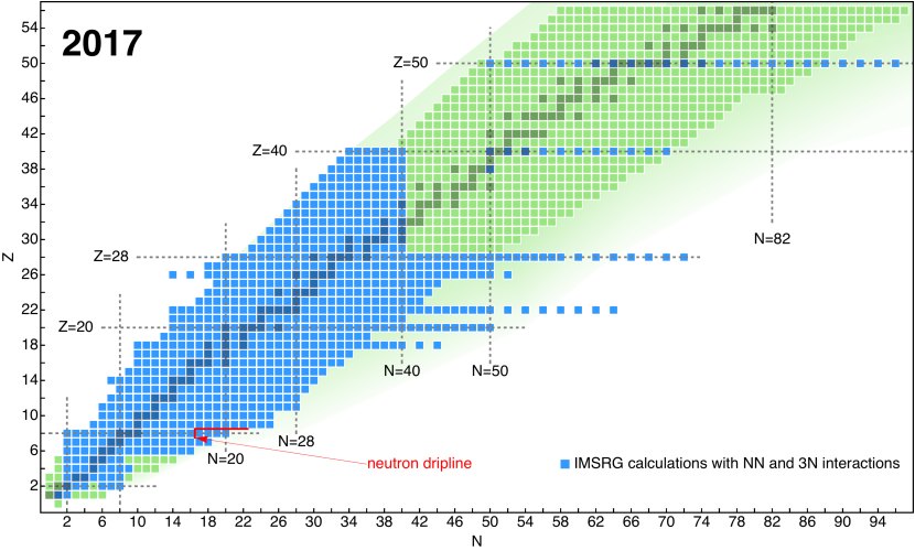
Figure 1: Survey of IMRSG-based calculations of nuclear ground-state properties and low-lying spectra up to 2017.

In the IMSRG, we apply the idea of decoupling energy scales to directly tackle the nuclear many-body problem [38, 39, 40, 37]. In essence, we use RG flow equations to decouple physics at different excitation energy scales of the nucleus, and render the Hamiltonian matrix in configuration space block or band diagonal in the process. With an appropriately chosen decoupling strategy, it is even possible to extract specific eigenvalues and eigenstates of the Hamiltonian, and thereby solve the quantum many-body problem. We will see that this can be achieved on the operator level, without actually constructing the Hamiltonian matrix in a factorially growing configuration space basis. We will also discuss how the IMSRG evolution can be viewed as a re-organization of the many-body expansion in which correlations are absorbed into an RG-improved Hamiltonian. The idea of using Hamiltonian flow equations to solve quantum many-body problems was already discussed in Wegner’s initial SRG work [26] (also see [41] and references therein), and it is used in a variety of flavors in domains like solid-state physics [42, 43, 44, 45, 46], or quantum chemistry [47, 48, 49, 50, 51, 52].

In the following, we will briefly discuss the salient elements of the chiral EFT description of the strong interaction at low energies (Sec. 2), and the use of SRG evolutions to dial the resolution scale of nuclear interactions (Sec. 3). We will then describe the IMSRG formalism and its extension to correlated reference states, with the specific goal of tackling open-shell systems with multi-reference character (Sec. 4). Selected applications of this Multireference IMSRG (MR-IMSRG) are presented in Sec. 5, followed by a discussion of how the MR-IMSRG can help us tackle collective correlations in nuclei (Sec. 6). Finally, we will touch upon the use of IMSRG-improved Hamiltonians in other many-body methods, and possible interfaces with White’s Density Matrix Renormalization Group (DMRG) [53], as well as tensor RG methods for many-body systems on spatial lattices [54, 55, 56] (Sec. 7).

2 Effective Field Theories of the Strong Interaction

Quantum Chromodynamics (QCD) is the fundamental theory of the strong interaction between quarks and gluons. One of its essential features is that the strength of the interaction increases in the low-energy domain that is most relevant for the structure and reactions of atomic nuclei [57, 58]. This makes the description of all but the lightest nuclei at the QCD level inefficient at best, and impossible at worst. However, strongly interacting matter undergoes a phase transition from a quark-gluon plasma to a hadronic phase in which quarks are confined in composite particles like nucleons and pions. These particles can be used as building blocks for an EFT of the strong interaction.

Following Weinberg [59, 60], the dynamics of an EFT are governed by a Lagrangian consisting of all interactions that are consistent with the symmetries of the underlying theory. Of particular importance is the chiral symmetry of QCD: massless QCD is invariant under independent rotations of left- and right-handed quarks (hence the name chiral symmetry), expressed by the symmetry group $SU(2)_{L}\times SU(2)_{R}$ [59, 61, 3]. This symmetry is explicitly broken by the quark mass terms, but since the masses of the up and down quarks are small, it is still very relevant for the interactions of nucleons and pions, which are built from those light quarks. Since the symmetry group $SU(2)_{L}\times SU(2)_{R}$ can be equivalently represented as a product of vector and axial vector rotations, $SU(2)_{V}\times SU(2)_{A}$, chiral symmetry would imply the existence of parity doublets of strongly interacting particles which are not found in nature. Thus, we can conclude that chiral symmetry must be broken spontaneously, and it turns out that it is the axial component of the theory that undergoes this symmetry breaking. The invariance of nuclear and nucleon-pion interactions under the remaining $SU(2)_{V}$ group is the well-known nuclear isospin symmetry [62]. The relevant particle multiplets for chiral EFT are the proton and neutron, as well as the $\pi_{+},\pi_{0},\pi_{-}$ mesons. The spontaneous breaking of chiral symmetry implies the existence of massless Goldstone bosons [63], which can be readily identified with the pions.

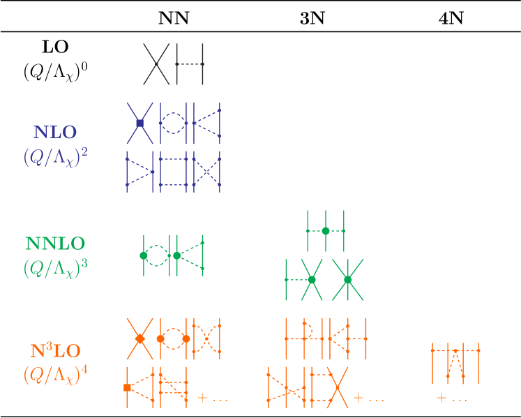
Figure 2: Chiral two-, three- and four nucleon forces through next-to-next-to-next-to-leading order (N³LO) (see, e.g., [2, 3, 6]). Dashed lines represent pion exchanges between nucleons. The large solid circles, boxes and diamonds represent vertices that are proportional to low-energy constants (LECs) of the theory (see text).

Another important consequence of chiral symmetry and its breaking is that only derivatives of the pion fields couple to the nucleon. Thus, interaction vertices (and Feynman diagrams) become proportional to ($q/\Lambda_{\chi}$), where $q\sim m_{\pi}\sim k_{F}\approx 140\,\,\text{MeV}/c$ is the typical momentum of a system of nucleons and pions, and $\Lambda_{\chi}$ is the so-called breakdown scale of the EFT. The breakdown scale is associated with physics that is not explicitly taken into account by the constructed EFT. In chiral EFT, $\Lambda_{\chi}$ is traditionally considered to be in the range $700-1000\,\,\text{MeV}$, with the lower value corresponding to the mass of the $\rho$ meson that is not an explicit degree of freedom of the theory. Assumptions about $\Lambda_{\chi}$ have come under increasing scrutiny as applications in medium-mass nuclei have revealed shortcomings of the chiral interactions (see, e.g., [64] and references therein).

Nevertheless, the proportionality of the interaction vertices to $q/\Lambda_{\chi}<1$ makes it possible to organize the chiral Lagrangian in powers of this ratio. Based on this power-counting scheme, one can then develop a systematic low-momentum expansion of nuclear interactions, as shown in Fig. 2 (see [59, 2, 3, 6]). These interactions consist of pion exchanges between nucleons, indicated by dashed lines, as well as nucleon contact interactions. Importantly, the diagrams shown in Fig. 2 contain different types of pion-nucleon, nucleon-nucleon, and three-nucleon vertices that are proportional to specific LECs of chiral EFT. As mentioned above, these LECs encode physics that is not explicitly resolved, either because it corresponds to a high momentum scale, or involves degrees of freedom that are not explicitly treated by the theory. Eventually, one hopes to calculate these LECs directly from the underlying QCD, i.e., through matching results from the nuclear sector to Lattice QCD calculations (see [15, 16] for first attempts in that direction). In the mean time, the LECs are fit to experimental data.

The organization of nuclear forces from leading (LO) to next-to-next-to-next-to-leading order (N³LO) and beyond in the chiral expansion is appealing for a number of reasons. By starting from a chiral Lagrangian, we obtain a consistent set of two-, three- and higher many-nucleon interactions, and the power counting explains the empirical hierarchy of these nuclear forces, i.e., $V_{\text{NN}}>V_{\text{3N}}>V_{\text{4N}}>\ldots$. Moreover, the chiral Lagrangian can be readily extended with couplings to the electroweak sector by replacing the derivatives with their gauge covariant versions. This implies that the same LECs appear in the nuclear interactions and electroweak currents, and the LECs can therefore be constrained by electroweak observables (see, e.g., [65, 11, 14, 12]). Last but not least, by truncating the chiral expansion at a given order, we will eventually be able to quantify the theoretical uncertainties of the interactions and operators that serve as input for nuclear many-body theory, once some persistent issues are resolved (see, e.g., [6, 66, 8, 9, 67, 68]).

3 The Similarity Renormalization Group

As mentioned in the introduction, RG methods are natural companions for EFTs, because they make it possible to smoothly dial the resolution scale of those theories. In low-energy nuclear physics, RG methods have played an important role in formalizing ideas on the renormalization of nuclear interactions and many-body effects that had been discussed by the community for a long time (see [21, 22, 23, 24] and references therein). For instance, local NN interactions with repulsive cores at short inter-particle distances or non-local interactions that reproduce NN scattering data equally well, can yield significantly different properties for nuclei and nuclear matter (see, e.g., [69, 70]). Colloquially, interactions with strong short-range repulsion are referred to as “hard” interactions because they induce strong many-body correlations that make the nuclear many-body problem non-perturbative. Coester and co-workers [69] showed that nuclear interactions can be softened via unitary transformations that shift strength from the repulsive core into non-local contributions, thereby making mean-field and finite-order beyond mean-field approximations to the many-body problem viable. While their work and similar investigations explicitly recognized that such transformations lead to induced many-body forces, those forces were neglected, and the discussion very much revolved around using these techniques to pin down the “true” nucleon-nucleon potential.

From the modern RG perspective, there is no such thing as a true potential, but rather infinitely many unitarily equivalent representations of low-energy QCD. In this context, the use of soft or hard NN interactions is related to the choice of a low or high resolution scale for the description of the nuclear many-body system. When an RG is used to dial the resolution, the induced many-body forces must be accounted for so that observables remain invariant under the RG flow (see below). For instance, induced 3N forces play a crucial role in obtaining proper nuclear matter saturation properties if we work at low resolution scale (see, e.g., [71, 72, 73]). Of course, 3N (and higher) forces are present anyway in an EFT treatment of the strong interaction, as discussed in the previous section.

3.1 SRG Evolution of Nuclear Forces

In Fig. 3 we show features of the central and tensor forces of the Argonne V18 (AV18) interaction [74] in the two-body spin-isospin channel $(S,T)=(1,0)$, which contains the deuteron bound state. AV18 is a so-called realistic interaction that describes NN scattering data with high accuracy, but precedes the modern chiral forces discussed above. It is specifically tailored to be as local as possible, to make it a suitable input for Quantum Monte Carlo calculations [75, 7, 8, 9]. This is the reason why AV18 has a strong repulsive core in the central part of the interaction. Like all NN interactions, it also has a tensor interaction resulting from pion exchange that mixes states with different orbital angular momenta,

$$V_{T}=v_{T}(r)S_{12}(r)\equiv\frac{v_{T}(r)}{r^{2}}\left(3(\vec{\sigma}_{1}\cdot\vec{r})(\vec{\sigma}_{2}\cdot\vec{r})-(\vec{\sigma}_{1}\cdot\vec{\sigma}_{2})r^{2}\right),$$ (1)

The radial dependencies of AV18’s central and tensor interactions are shown in the left panel of Fig. 3. In the corresponding momentum representation, the ${}^{3}S_{1}$ partial wave has strong off-diagonal matrix elements, with tails extending to relative momenta as high as $|\vec{q}|\sim 20\,\,\text{fm}^{-1}$. The matrix elements of the ${}^{3}S_{1}-{}^{3}D_{1}$ mixed partial wave, which are generated exclusively by the tensor force, are sizable as well. The strong coupling between states with low and high relative momenta forces us to use large Hilbert spaces in few- and many-body calculations, even if we are only interested in the lowest eigenstates. Consequently, the eigenvalues and eigenstates of the nuclear Hamiltonian converge very slowly with respect to the basis size of the Hilbert space (see, e.g., [30]). To solve this problem, we can perform an RG evolution of the NN interaction.

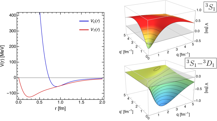
Figure 3: Repulsive core and tensor force of the Argonne V18 NN interaction [74] in the $(S,T)=(1,0)$ channel. In the left panel, the radial dependencies of the central ($V_{C}(r)$) and tensor components ($V_{T}(r)$) of Argonne V18 are shown, while the right panel shows its momentum space matrix elements in the deuteron partial waves.

First systematic applications of RG methods for the renormalization of nuclear interactions were based on RG decimation, i.e., the projection of the Hamiltonian onto a low-momentum (low-energy) subspace (see [21, 23] and references therein). In recent years, however, the so-called Similarity Renormalization Group (SRG) has become the RG method of choice in nuclear physics [25, 26, 23]. The SRG is based on unitary transformations rather than projection methods, which greatly facilitates the construction of observables that are consistent with the renormalized interaction.

The basic concept of the SRG is more general than required by RG theory: We aim to simplify the structure of the Hamiltonian in a suitable representation through a continuous unitary transformation,

$$H(s)=U(s)H(0){{U}}^{{\dagger}}(s)\,.$$ (2)

Here, $H(s=0)$ is the starting Hamiltonian, and the flow parameter $s$ parameterizes the unitary transformation. To implement this transformation, we take the derivative of Eq. (2) to obtain the operator flow equation

$$\frac{d{}}{d{s}}H(s)=[{\eta(s)},{H(s)}]\,,$$ (3)

where the anti-Hermitian generator $\eta(s)$ is related to $U(s)$ by

$$\eta(s)=\frac{d{U(s)}}{d{s}}U^{{\dagger}}(s)=-\eta^{{\dagger}}(s)\,.$$ (4)

We can choose $\eta(s)$ to transform the Hamiltonian to almost arbitrary structures as we integrate the flow equation (3) for $s\to\infty$. Wegner [26] proposed the generator

$$\eta(s)\equiv[{H_{d}(s)},{H_{od}(s)}]\,,$$ (5)

which is constructed by splitting the Hamiltonian into suitably chosen diagonal ($H_{d}(s)$) and off-diagonal ($H_{od}(s)$) parts. The generator (5) will then suppress $H_{od}(s)$ as the Hamiltonian is evolved via equation (3) (see [26, 41, 23, 40, 37]). Here, the label diagonal merely refers to a desired structure that the Hamiltonian will assume in the limit $s\to\infty$, and not strict diagonality. We can make contact with renormalization ideas by imposing a block or band-diagonal structure on the Hamiltonian that implies a decoupling of momentum or energy scales in the RG sense.

Figure 4: SRG evolution of the chiral N³LO NN interaction by Entem and Machleidt [76, 3]. In the left column, we show the momentum-space matrix elements of the interaction in the ${}^{3}S_{1}$ partial wave for different values of the SRG resolution scale $\lambda$. The top-most row shows the initial interaction at $s=0\,\,\text{fm}^{4}$ , i.e., “$\lambda=\infty$”. In the right column, we show the $S-$ and $D-$wave components of the deuteron wave function that is obtained by solving the Schrödinger equation with the corresponding SRG-evolved interaction.

As an example of a realistic application, Fig. 4 shows the SRG evolution of a chiral N³LO NN interaction. We use a Wegner-type generator built from the relative kinetic energy in the two-nucleon system to drive the Hamiltonian towards a band-diagonal structure in momentum space:

$$\eta(\lambda)\equiv\Big{[}\,\frac{\vec{q}^{2}}{2\mu},v(\lambda)\Big{]}\,.$$ (6)

We have changed variables from the flow parameter $s$ to $\lambda=s^{-1/4}$, which has the dimensions of a momentum (in natural units), for reasons that will become clear shortly.

We start from the matrix elements of the initial interaction in the ${}^{3}S_{1}$ partial wave that are shown in the top row. The interaction has no appreciable strength in states with momentum differences $|\Delta\vec{q}|=|\vec{q}^{\prime}-\vec{q}|\gtrsim 4.5\,\,\text{fm}^{-1}$. By evolving the initial interaction to $\lambda=3\,\,\text{fm}^{-1}$ and then to $2\,\,\text{fm}^{-1}$, the off-diagonal matrix elements are suppressed, and the interaction is almost entirely contained in a block of states with $|\Delta\vec{q}|\sim 2\,\,\text{fm}^{-1}$, except for a weak diagonal ridge. Thus, we see that $\lambda$ limits the momentum that the interaction can transfer between pairs of nucleons, and we identify $\lambda$ with the resolution scale of the evolved interaction.

Next to the matrix elements, we show deuteron wave functions obtained by solving the Schrödinger equation with Hamiltonian at each $\lambda$. For the initial interaction, the $S-$wave ($L=0$) component of the wave function is suppressed at small relative distances, which reflects short-range correlations between the nucleons. There is also a significant $D-$wave ($L=2$) admixture due to the tensor interaction. As we lower the resolution scale, the “correlation hole” in the wave function is eliminated, and the $D-$wave admixture is reduced because the evolution suppresses the ${}^{3}S_{1}-{}^{3}D_{1}$ matrix elements that cause this mixing [23]. The structure of the wave function becomes very simple, reminiscent of a Gaussian ansatz for a pair of independent nucleons.

3.2 Induced Forces

The RG decoupling of low- and high-lying momenta prevents the Hamiltonian from scattering nucleon pairs from low- to high-momentum states, which makes it possible to converge many-body calculations in much smaller Hilbert spaces than for the harder initial interactions [77, 30, 31, 33, 32, 39, 78, 40, 79, 80, 81, 34, 82, 83, 84, 85]. However, this improvement comes at a cost, which is best illustrated by considering the Hamiltonian in second-quantized form, assuming only a two-nucleon interaction for simplicity:

$$H_{\text{int}}=T_{\text{rel}}+V=\frac{1}{4}\sum_{pqrs}\langle{pq}|\,{\frac{\vec{q}_{12}^{\,2}}{2\mu}+v_{12}}\,|{rs}\rangle{{a}}^{{\dagger}}_{p}{{a}}^{{\dagger}}_{q}a_{s}a_{r}\,.$$ (7)

Inserting $T_{\text{rel}}$ and $V$ into Eqs. (6) and (3), we obtain

$$[{{{a}}^{{\dagger}}_{i}{{a}}^{{\dagger}}_{j}a_{l}a_{k}},{{{a}}^{{\dagger}}_{p}{{a}}^{{\dagger}}_{q}a_{s}a_{r}}]=\delta_{lp}{{a}}^{{\dagger}}_{i}{{a}}^{{\dagger}}_{j}{{a}}^{{\dagger}}_{q}a_{s}a_{r}a_{k}+\{{{a}}^{{\dagger}}{{a}}^{{\dagger}}{{a}}^{{\dagger}}aaa\}-\delta_{lp}\delta_{kq}{{a}}^{{\dagger}}_{i}{{a}}^{{\dagger}}_{j}a_{s}a_{r}+\{{{a}}^{{\dagger}}{{a}}^{{\dagger}}aa\}\,,$$ (8)

where the terms in brackets schematically stand for additional two- and three-body operators. Thus, even if we start from a pure two-body interaction, the SRG flow will induce operators of higher rank.

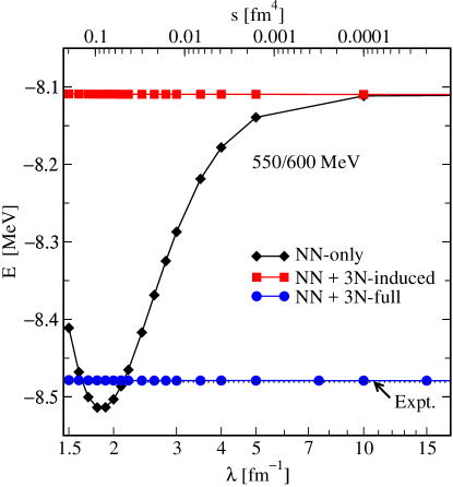
Figure 5: Ground state energy of ${}^{3}\mathrm{H}$ as a function of the flow parameter $\lambda$ for chiral NNLO $NN$ and $NN\!+\!3N$ interactions (see [86] for details). $NN$-only means initial and induced $3N$ interactions are discarded, $NN\!+\!3N$-induced takes only induced $3N$ interactions into account, and $3N$-full contains initial $3N$ interactions as well. The black dotted line shows the experimental binding energy [87]. Data for the figure courtesy of K. Hebeler.

Nowadays, state-of-the-art SRG evolutions of nuclear interactions are performed in the three-body system [88, 89, 31, 86, 90]. In Fig. 5, we show ${}^{3}\mathrm{H}$ ground-state energies that have been calculated with a family of SRG-evolved interactions that is generated from chiral NN and NN+3N interactions (see [86] for full details). If we truncate the evolved interaction and the SRG generator at the two-body level (NN-only), the SRG evolution is not unitary in the 3N system and the energy becomes $\lambda$ dependent. If we truncate the operators at the three-body level instead, induced 3N interactions are properly included and unitarity is restored (NN+3N-induced): The energy does not change as $\lambda$ is varied. Finally, for the curve NN+3N-full a 3N force is included in the initial Hamiltonian and evolved consistently. The resulting triton ground-state energy is invariant under the SRG flow, and it closely reproduces the experimental value because the 3N interaction’s LECs are fit accordingly [2, 3, 65].

The triton example shows that it is important to track induced interactions, especially if we want to use evolved nuclear Hamiltonians as input for medium-mass or heavy nuclei rather than the few-nucleon system considered so far. The nature of the SRG works at least somewhat in our favor, because truncations of the SRG flow equations lead to a violation of unitarity that manifests as a (residual) dependence of observables on the resolution scale $\lambda$. We can use this dependence as a tool to assess the size of missing contributions, although one has to take great care to disentangle them from the effects of many-body truncations [23, 88, 86, 77, 39, 32, 34, 85, 91]. The empirical observation that SRG evolutions to resolutions as low as $\lambda\sim 1.5\,\text{fm}^{-1}$ appear to preserve the natural hierarchy of nuclear forces, i.e., $V_{\text{NN}}>V_{\text{3N}}>V_{\text{4N}}>\ldots$, suggests that we can truncate induced forces whose contributions would be smaller than the desired accuracy of our calculations.

4 The In-Medium SRG

4.1 Concept

As discussed in Sec. 3, the concept of the SRG is actually quite general: We can use continuous unitary transformations to drive a given Hamiltonian (or generic operator) to a desired structure, defined by our choice of the diagonal and off-diagonal parts of the Hamiltonian, $H_{d}$ and $H_{od}$. If we choose $H_{d}$ to be the diagonal entries of a system’s Hamiltonian matrix, the SRG would amount to solving the eigenvalue problem! If we consider applying this idea in genuine many-body systems like medium-mass or heavy nuclei, we quickly realize that an SRG evolution of the many-body Hamiltonian matrix would be a very inefficient approach for solving the Schrödinger equation, because the RHS of Eq. (3) forces us to repeatedly perform products of matrices whose dimension grows factorially with the number of particles and single-particle basis states. Moreover, we would essentially be working to obtain the complete spectrum of that large matrix representation rather than just a comparably small number of low-lying states that we are truly interested in.

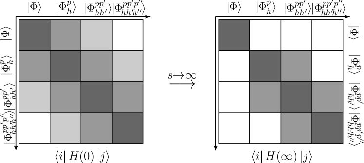
Figure 6: Schematic view of IMSRG decoupling in a many-body Hilbert space spanned by a Slater determinant reference $\,|{\Phi}\rangle$ and its particle-hole excitations $\,|{\Phi^{p\ldots}_{h\ldots}}\rangle$.

Instead of this naive approach, we can evolve the Hamiltonian operator, and achieve the desired decoupling without ever constructing a large matrix. To this end, let us consider a representation of the Hamiltonian in a basis built from a reference Slater determinant $\,|{\Phi}\rangle$ and its particle-hole excitations, as shown in the left panel of Fig. 6. For simplicity, we show a two-body Hamiltonian, which can at most couple the reference state $\,|{\Phi}\rangle$ to 2p2h excitations, and in general $n$p$n$h to $(n\pm 2)$p$(n\pm 2)$h states, yielding the schematic band structure on display. We now want to continuously evolve this Hamiltonian to the shape shown in the right panel of Fig. 6. Inspecting the evolved Hamiltonian more closely, we see that we aim to decouple the matrix element $\langle{\Phi}|\,{H(s)}\,|{\Phi}\rangle$ from all excitations in the limit $s\to\infty$ — if we succeed, we will have extracted an eigenvalue of $H$, and our unitary transformation will provide us with a mapping of the Slater determinant $\,|{\Phi}\rangle$ onto an exact eigenstate $\,|{\Psi}\rangle$ of $H(0)$, typically the ground state.

Since we are working with a reference state and its excitations, it is convenient to represent the Hamiltonian in terms of normal-ordered operators. We introduce the compact notation

$$A^{i_{1}\ldots i_{k}}_{j_{1}\ldots j_{k}}\equiv{{a}}^{{\dagger}}_{i_{1}}\ldots{{a}}^{{\dagger}}_{i_{k}}a_{j_{k}}\ldots a_{j_{1}}\,$$ (9)

for strings of creation and annihilation operators, and the normal ordered operators

$$:\!A^{i}_{k}: =A^{i}_{k}-\rho^{i}_{k}$$ (10)

$$:\!A^{ij}_{kl}: =A^{ij}_{kl}-:\!A^{i}_{k}:\rho^{j}_{l}+\text{perm.}-\rho^{i}_{k}\rho^{j}_{l}+\text{perm.}$$ (11)

$$\ldots\,$$

where $\rho^{i}_{k}=\langle{\Phi}|\,{A^{i}_{k}}\,|{\Phi}\rangle$ is the usual one-body density matrix of the reference state (see [40, 37] for details). An intrinsic nuclear $A$-body Hamiltonian with NN and 3N interactions,

$$H=T-T_{\text{cm}}+V_{2}+V_{3}$$ (12)

can then be exactly rewritten as

$$H =E+\sum_{ij}f^{i}_{j}:\!A^{i}_{j}:+\frac{1}{4}\sum_{ijkl}\Gamma^{ij}_{kl}:\!A^{ij}_{kl}:+\frac{1}{36}\sum_{ijklmn}W^{ijk}_{lmn}:\!A^{ijk}_{lmn}:\,,$$ (13)

with the individual zero- through three-body contributions

$$E \equiv\left(1-\frac{1}{A}\right)\sum_{ab}t^{a}_{b}\rho^{a}_{b}+\frac{1}{4}\sum_{abcd}\left(\frac{1}{A}t^{ab}_{cd}+v^{ab}_{cd}\right)\rho^{ab}_{cd}+\frac{1}{36}\sum_{abcdef}v^{abc}_{def}\rho^{abc}_{def}\,,$$ (14)

$$f^{i}_{j} \equiv\left(1-\frac{1}{A}\right)t^{i}_{j}+\sum_{ab}\left(\frac{1}{A}t^{ia}_{jb}+v^{ia}_{jb}\right)\rho^{a}_{b}+\frac{1}{4}\sum_{abcd}v^{iab}_{jcd}\rho^{ab}_{cd}\,,$$ (15)

$$\Gamma^{ij}_{kl} \equiv\frac{1}{A}t^{ij}_{kl}+v^{ij}_{kl}+\sum_{ab}v^{ija}_{klb}\rho^{a}_{b}\,,$$ (16)

$$W^{ijk}_{lmn} \equiv v^{ijk}_{lmn}\,.$$ (17)

Here, $\rho^{a\ldots}_{i\ldots}=\langle{\Phi}|\,{A^{i_{1}\ldots i_{k}}_{j_{1}\ldots j_{k}}}\,|{\Phi}\rangle$ denote the $k$-body density matrices of the reference state. For reasons that will become clear below, we refrain from simplifying these expressions by using the factorization of Slater determinant’s density matrices. We note that due to the normal ordering, the zero-, one-, and two-body coefficients all contain in-medium contributions from the three-body interaction, i.e., contractions of three-body matrix elements with the density matrices of the reference state. This explains the name In-Medium SRG, and will play an important role when we introduce truncations of the IMSRG flow equations below.

Using this definition of the Hamiltonian, we can use Wick’s theorem to evaluate the many-body matrix elements that couple $\,|{\Phi}\rangle$ to excitations, i.e.,

$$\langle{\Phi^{p}_{h}}|\,{:\!H:}\,|{\Phi}\rangle =\langle{\Phi}|\,{:\!A^{h}_{p}::\!H:}\,|{\Phi}\rangle=f^{p}_{h}$$ (18)

$$\langle{\Phi^{pp^{\prime}}_{hh^{\prime}}}|\,{:\!H:}\,|{\Phi}\rangle =\langle{\Phi}|\,{:\!A^{hh^{\prime}}_{pp^{\prime}}::\!H:}\,|{\Phi}\rangle=\Gamma^{pp^{\prime}}_{hh^{\prime}}\,$$ (19)

(see [40, 37]). These matrix elements define our off-diagonal Hamiltonian

$$H_{od}\equiv\sum_{ph}f^{p}_{h}:\!A^{p}_{h}:+\frac{1}{4}\sum_{pp^{\prime}hh^{\prime}}\Gamma^{pp^{\prime}}_{h^{\prime}h}:\!A^{pp^{\prime}}_{hh^{\prime}}:+\text{H.c.}\,,$$ (20)

which can then be used in Eq. (5) or another suitable ansatz for the generator (see [40, 37] for details) to evolve the Hamiltonian to the desired form shown in the right panel of Fig. 6. Note that the elimination of $H_{od}$ also removes the couplings between general $n$p$n$h and $(n\pm 2)$p$(n\pm 2)$h states, i.e., the outermost side-diagonal blocks.

4.2 Correlated Reference States

The discussion so far was based on the use of a Slater determinant as the reference state. On the one hand, such an independent-particle reference is convenient because it allows us to distinguish particle and hole states in our single-particle basis, but on the other hand, it means that the unitary transformation must encode all many-body correlations. The unitarity of the IMSRG transformation offers us more flexibility, because we can control to what extent correlations are described by either the Hamiltonian or the reference state. To see this, we consider the stationary Schrödinger equation and apply $U(s)$:

$$\left[U(s)H{{U}}^{{\dagger}}(s)\right]U(s)\,|{\Psi_{k}}\rangle=E_{k}U(s)\,|{\Psi_{k}}\rangle\,.$$ (21)

$U(s)$ shifts correlations from the wave function into the evolved, RG-improved Hamiltonian $H(s)=U(s)H{{U}}^{{\dagger}}(s)$. In many-body calculations with this Hamiltonian, the many-body method now “only” needs to approximate $U(s)\,|{\Psi_{k}}\rangle$ rather than $\,|{\Psi_{k}}\rangle$ — in the case discussed so far, even a Slater determinant would be sufficient because $U(s)$ or $H(s)$ describe the correlations. There can be situations in which it is worthwhile to use the reference state to describe certain types of correlations, especially if it can capture them more efficiently than through the particle-hole type expansion in which the IMSRG-evolved Hamiltonian is set up (see Sec. 6).

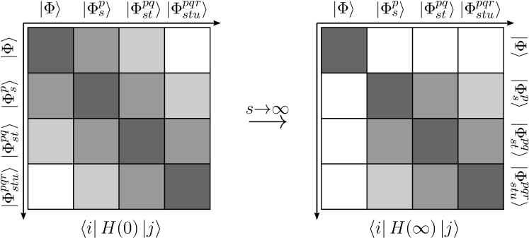
Figure 7: Schematic view of MR-IMSRG decoupling in the many-body Hilbert space. $\,|{\Phi}\rangle$ denotes an arbitrary reference state, and $\,|{\Phi^{p\ldots}_{s\ldots}}\rangle$ are suitably defined excitations.

The IMSRG framework can be extended to correlated reference states using a generalized normal ordering developed by Kutzelnigg and Mukherjee [92, 93]. It requires a new ingredient, the irreducible $k$-body density matrices $\lambda^{(k)}$. In the one-body case, this is just the usual density matrix

$$\lambda^{i}_{k}\equiv\rho^{i}_{k}=\langle{\Phi}|\,{A^{i}_{k}}\,|{\Phi}\rangle\,,$$ (22)

while for $k\geq 2$,

$$\lambda^{ij}_{kl} \equiv\rho^{ij}_{kl}-\mathcal{A}\{\lambda^{i}_{k}\lambda^{j}_{l}\}\,,$$ (23)

$$\lambda^{ijk}_{lmn} \equiv\rho^{ijk}_{lmn}-\mathcal{A}\{\lambda^{i}_{l}\lambda^{jk}_{mn}\}-\mathcal{A}\{\lambda^{i}_{l}\lambda^{j}_{m}\lambda^{k}_{n}\}\,,$$ (24)

etc., where $\mathcal{A}\{\ldots\}$ fully antisymmetrizes the indices of the expression within the brackets. The irreducible densities encode the correlation content of an arbitrary reference state $\,|{\Phi}\rangle$. If the reference state is a Slater determinant, i.e., an independent-particle state, the full two-body density matrix factorizes, and $\lambda^{(2)}$ vanishes (see, e.g., [37]).

Normal-ordered one-body operators are constructed in the same manner as in the standard normal ordering, e.g.,

$$:\!A^{a}_{b}: =A^{a}_{b}-\lambda^{a}_{b}\,,$$ (25)

$$:\!A^{ab}_{cd}: =A^{ab}_{cd}-\lambda^{a}_{c}:\!A^{b}_{d}:+\lambda^{a}_{d}:\!A^{b}_{c}:-\lambda^{b}_{d}:\!A^{a}_{c}:+\lambda^{b}_{c}:\!A^{a}_{d}:-\lambda^{a}_{c}\lambda^{b}_{d}+\lambda^{a}_{d}\lambda^{b}_{c}-\lambda^{ab}_{cd}\,,$$ (26)

$$\ldots$$

The expressions for the coefficients of the normal-ordered nuclear Hamiltonian, Eqs. (14)–(17) remain unchanged, because we wrote them in terms of the full density matrices. When we work with arbitrary reference states, the regular Wick’s theorem extended with additional contractions like

$$:\!A^{\framebox{\scriptsize$ab$}}_{cd}::\!A^{ij}_{\framebox{\scriptsize$kl$}}: =+\lambda^{\framebox{\scriptsize$ab$}}_{\framebox{\scriptsize$kl$}}:\!A^{ij}_{cd}:\,,$$ (27)

$$:\!A^{\framebox{\scriptsize$ab$}}_{c\framebox{\scriptsize$d$}}::\!A^{\framebox{\scriptsize$i$}j}_{\framebox{\scriptsize$kl$}}: =-\lambda^{\framebox{\scriptsize$abi$}}_{\framebox{\scriptsize$dkl$}}:\!A^{j}_{c}:\,,$$ (28)

$$:\!A^{\framebox{\scriptsize$ab$}}_{\framebox{\scriptsize$cd$}}::\!A^{\framebox{\scriptsize$ij$}}_{\framebox{\scriptsize$kl$}}: =+\lambda^{\framebox{\scriptsize$abij$}}_{\framebox{\scriptsize$cdkl$}}\,.$$ (29)

(see [37] for a detailed discussion). These contractions increase the number of terms when we expand operator products, e.g., in the analysis of many-body matrix elements or the flow equations (see below), but fortunately, the overall increase in complexity is manageable.

In Fig. 7, we illustrate the schematic decoupling for the Hamiltonian in a basis spanned by a correlated reference state and its excitations. Since our reference state is no longer a Slater determinant, there are no well-defined notions of a Fermi surface or particle and hole states any longer, and the indices of the excitation operators run over all single-particle states instead. Per construction, the reference state $\,|{\Phi}\rangle$ is still orthogonal to general excitations $:\!A^{i_{1}\ldots i_{k}}_{j_{1}\ldots j_{k}}:\,|{\Phi}\rangle$ because

$$\langle{\Phi}|\,{:\!A^{i_{1}\ldots i_{k}}_{j_{1}\ldots j_{k}}:}\,|{\Phi}\rangle\,.$$ (30)

The excitations themselves, however, are in general not orthogonal to each other, and may even be linearly dependent. As a result, the structure of the evolved MR-IMSRG Hamiltonian, shown in the right panel of Fig. 7, is not simplified as much as in the Slater determinant case, since matrix elements in the outer diagonals are not necessarily removed when novel contractions like (27)–(29) are in play.

In the MR-IMSRG, the linear dependence implies that we are implicitly transforming a rank-deficient many-body Hamiltonian matrix and are possibly working harder than we need to by dragging along a space of spurious eigenstates with zero eigenvalues. Since the nuclear states we are interested in have absolute binding energies of several hundred MeVs, there has been no evidence that the presence of these spurious eigenstates adversely affects the physical states in practical calculations.

4.3 MR-IMSRG Flow Equations

We are now ready to formulate the MR-IMSRG flow equations by applying the generalized normal ordering and Wick’s theorem to Eq. (3). We express all operators in terms of normal-ordered strings of creation and annihilation operators. As discussed in Sec. 3, each evaluation of the commutator in Eq. (3) induces operators of higher rank,

$$[{:\!A^{ab}_{cd}:},{:\!A^{ij}_{kl}:}]=\delta_{ci}:\!A^{abj}_{dkl}:+\ldots,$$ (31)

hence we need to introduce truncations to obtain a computationally feasible many-body method. In contrast to Eq. (8), we are now working with normal-ordered operators whose in-medium contributions have been absorbed into terms of lower rank and we expect the induced operators to be much weaker than in the free-space SRG case. There is ample empirical evidence that the residual normal-ordered three-body piece can be neglected to a very good approximation in nuclear physics [94, 80, 37]. In our framework, we will eventually have to consider how the truncated terms may feed back into operators of lower rank as we evolve the flow equations (see below). In practice, we presently truncate all flowing operators at the two-body level to close the system of flow equations:

$$\eta(s) \approx\eta^{(1)}(s)+\eta^{(2)}(s)\,,$$ (32)

$$H(s) \approx E(s)+f(s)+\Gamma(s)\,,$$ (33)

$$\frac{d{}}{d{s}}H(s) \approx\frac{d{}}{d{s}}E(s)+\frac{d{}}{d{s}}f(s)+\frac{d{}}{d{s}}\Gamma(s)\,.$$ (34)

This is the so-called MR-IMSRG(2) truncation [38, 95, 39, 32, 78, 96, 40], which is a cousin to a variety of other truncated many-body schemes, in particular Coupled Cluster with Singles and Doubles excitations (CCSD) [97, 35, 47, 98, 48, 49, 99, 50, 100, 101, 102, 51], although the latter is based on non-unitary similarity transformations.

The MR-IMSRG(2) flow equations are given by [32, 78, 37]

$$\frac{d{E}}{d{s}} =\sum_{ab}(n_{a}-n_{b})\eta^{a}_{b}f^{b}_{a}+\frac{1}{4}\sum_{abcd}\left(\eta^{ab}_{cd}\Gamma^{cd}_{ab}-\Gamma^{ab}_{cd}\eta^{cd}_{ab}\right)n_{a}n_{b}\bar{n}_{c}\bar{n}_{d}$$

$$\hphantom{=}+\frac{1}{4}\sum_{abcd}\left(\frac{d{}}{d{s}}\Gamma^{ab}_{cd}\right)\lambda^{ab}_{cd}+\frac{1}{4}\sum_{abcdklm}\left(\eta^{ab}_{cd}\Gamma^{kl}_{am}-\Gamma^{ab}_{cd}\eta^{kl}_{am}\right)\lambda^{bkl}_{cdm}\,,$$ (35)

$$\frac{d{}}{d{s}}f^{i}_{j} =\sum_{a}\left(\eta^{i}_{a}f^{a}_{j}-f^{i}_{a}\eta^{a}_{j}\right)+\sum_{ab}\left(\eta^{a}_{b}\Gamma^{bi}_{aj}-f^{a}_{b}\eta^{bi}_{aj}\right)(n_{a}-n_{b})$$

$$\hphantom{=}+\frac{1}{2}\sum_{abc}\left(\eta^{ia}_{bc}\Gamma^{bc}_{ja}-\Gamma^{ia}_{bc}\eta^{bc}_{ja}\right)\left(n_{a}\bar{n}_{b}\bar{n}_{c}+\bar{n}_{a}n_{b}n_{c}\right)$$

$$\hphantom{=}+\frac{1}{4}\sum_{abcde}\left(\eta^{ia}_{bc}\Gamma^{de}_{ja}-\Gamma^{ia}_{bc}\eta^{de}_{ja}\right)\lambda^{de}_{bc}+\sum_{abcde}\left(\eta^{ia}_{bc}\Gamma^{be}_{jd}-\Gamma^{ia}_{bc}\eta^{be}_{jd}\right)\lambda^{ae}_{cd}$$

$$\hphantom{=}-\frac{1}{2}\sum_{abcde}\left(\eta^{ia}_{jb}\Gamma^{cd}_{ae}-\Gamma^{ia}_{jb}\eta^{cd}_{ae}\right)\lambda^{cd}_{be}+\frac{1}{2}\sum_{abcde}\left(\eta^{ia}_{jb}\Gamma^{bc}_{de}-\Gamma^{ia}_{jb}\eta^{bc}_{de}\right)\lambda^{ac}_{de}\,,$$ (36)

$$\frac{d{}}{d{s}}\Gamma^{ij}_{kl} =\sum_{a}\left(\eta^{i}_{a}\Gamma^{aj}_{kl}+\eta^{j}_{a}\Gamma^{ia}_{kl}-\eta^{a}_{k}\Gamma^{ij}_{al}-\eta^{a}_{l}\Gamma^{ij}_{ka}-f^{i}_{a}\eta^{aj}_{kl}-f^{j}_{a}\eta^{ia}_{kl}+f^{a}_{k}\eta^{ij}_{al}+f^{a}_{l}\eta^{ij}_{ka}\right)$$

$$\hphantom{=}+\frac{1}{2}\sum_{ab}\left(\eta^{ij}_{ab}\Gamma^{ab}_{kl}-\Gamma^{ij}_{ab}\eta^{ab}_{kl}\right)\left(1-n_{a}-n_{b}\right)$$

$$\hphantom{=}+\sum_{ab}(n_{a}-n_{b})\left(\left(\eta^{ia}_{kb}\Gamma^{jb}_{la}-\Gamma^{ia}_{kb}\eta^{jb}_{la}\right)-\left(\eta^{ja}_{kb}\Gamma^{ib}_{la}-\Gamma^{ja}_{kb}\eta^{ib}_{la}\right)\right)\,,$$ (37)

where the $s$-dependence has been suppressed for brevity. We work in the natural orbital basis obtained by diagonalizing the one-body density matrix,

$$\lambda^{i}_{k}=n_{i}\delta^{i}_{k}\,,$$ (38)

where $0\leq n_{i}\leq 1$ indicates the occupation of the i-th orbital in the correlated reference state. Analogously, $0\leq\bar{n}_{i}=1-n_{i}\leq 1$ are the eigenvalues of the hole density matrix

$$\xi^{i}_{j}\equiv\lambda^{i}_{j}-\delta^{i}_{j}\,.$$ (39)

Note that due to the use of general reference states, the MR-IMSRG flow equations also include couplings to correlated pairs and triples of nucleons in the reference state through the irreducible density matrices $\lambda^{(2)}$ and $\lambda^{(3)}$. The single-reference limit for a Slater determinant reference state can be obtained by setting the irreducible density matrices $\lambda^{(2)}$ and $\lambda^{(3)}$ to zero, and noting that the occupation numbers now become either 0 or 1.

Superficially, the computational cost for the evaluation of the MR-IMSRG(2) flow equations is dominated by the final term of Eq. (35), which is of $\mathcal{O}(N^{7})$, where $N$ is the size of the single-particle basis. However, most practical ansätze for correlated reference states impose conditions on the density matrix that strongly limit the number of non-zero matrix elements. For instance, the particle-number projected Hartree-Fock-Bogoliubov (HFB) [103] reference states used in our initial applications (see Sec. 5) have almost diagonal $\lambda^{(k)}$ matrices. Moreover, relevant correlations are often restricted to a so-called valence or active space consisting of a small number of single-particle states, so that only density matrix elements with all indices belonging to this space are non-zero. Thus, the main driver of the computational effort is the integration of the two-body flow equation, at $\mathcal{O}(N^{6})$, which is the same naive scaling as for CCSD and similar methods. For closed-shell references, we can exploit the distinction of particle and hole indices to achieve exactly the same scaling as for single-reference CCSD theory, namely $\mathcal{O}(N_{h}^{2}N_{p}^{4})$.

5 Selected Applications

5.1 Reshuffling of Ground-State Correlations: ${}^{40}\mathrm{Ca}$

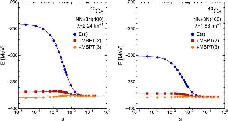
Figure 8: IMSRG(2) flow for ${}^{40}\mathrm{Ca}$ for a chiral NN+3N interaction, denoted NN+3N(400) in the following, at two different resolution scales $\lambda=2.24\,\text{fm}^{-1}$ and $1.88\,\text{fm}^{-1}$ (see Refs. [37, 40] for details). We show the flowing ground-state energy $E(s)$, and the sum of $E(s)$ and perturbative energy corrections evaluated with the evolving Hamiltonian $H(s)$ to illustrate the re-shuffling of correlations into the Hamiltonian (see text). The dashed lines indicate the final IMSRG(2) energies.

To illustrate the effect of the (MR-)IMSRG flow in practice, we first consider a ground-state calculation for the closed-shell nucleus ${}^{40}\mathrm{Ca}$. As our reference, we use a Slater determinant that is optimized by performing a Hartree-Fock calculation with a chiral NN+3N interaction. Figure 8 shows the IMSRG(2) ground-state energy $E(s)$ of ${}^{40}\mathrm{Ca}$ as a function of the flow parameter, which corresponds to the zero-body piece of the evolved normal-ordered Hamiltonian, Eq. (14). As we integrate the flow equations to increasing $s$, the Hamiltonian is RG-improved with correlations that are otherwise only accessible with post-Hartree Fock methods (see Refs. [40, 37] for details). This is evident if we also consider the size of the second and third-order MBPT energy corrections, evaluated with $H(s)$. After a few integration steps, the energy corrections are absorbed into the Hamiltonian, which implies that we could perform a Hartree-Fock calculation with $H(s)$ and obtain the fully correlated ground-state energy, up to truncation errors!

Figure 8 also illustrates that the size of the MBPT corrections depends significantly on the resolution scale of the Hamiltonian (see Sec. 3). At the higher resolution scale $\lambda=2.24\,\,\text{fm}^{-1}$, we gain about $130\,\,\text{MeV}$ of binding energy from correlations. At the lower resolution $\lambda=1.88\,\,\text{fm}^{-1}$, the HF reference state is already significantly lower in energy, so the energy gains from many-body correlations are less pronounced. This behavior is expected as interactions become increasingly soft, and thereby more perturbative (see, e.g., [23, 29]). Note that the final ground-state energies for $\lambda=2.24\,\,\text{fm}^{-1}$ and $1.88\,\,\text{fm}^{-1}$ are almost identical. As discussed in section 3, all results should ideally be invariant under arbitrary changes of $\lambda$, which seems to be the case for the specific NN+3N Hamiltonian we used here [77, 33].

5.2 Ground-State Energies Along Isotopic Chains: The Oxygen Isotopes

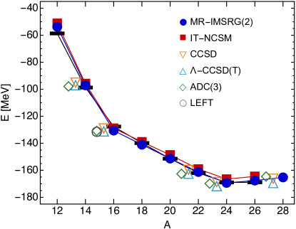
Figure 9: Ground-state energies of the oxygen isotopes from MR-IMSRG(2) and other many-body approaches, using the NN+3N(400) interaction at $\lambda=1.88\,\text{fm}^{-1}$. Some data points were offset horizontally to enhance the readability of the figure. The ADC(3) Self-Consistent Green’s Function results [104, 105] were obtained for $\lambda=2.0\,\,\text{fm}^{-1}$, but the dependence of energies on $\lambda$ is very weak (see Fig. 8). Black bars indicate experimental data [87].

The oxygen isotopic chain is an important testing ground for ab initio nuclear structure theory because it is accessible to a wide array of exact and approximate many-body methods [106, 77, 107, 32, 104, 108, 105, 109, 110, 111]. As a bonus, the semi-magicity of the oxygen isotopes — the $Z=8$ protons are in a closed-shell configuration — allows us to exploit spherical symmetry in our calculations. In Fig. 9, we compare MR-IMSRG(2) ground-state energies, obtained using particle-number projected HFB vacua [32, 112, 103] as references for the open-shell nuclei, with a variety of other methods:

• the Importance-Truncated No-Core Shell Model (IT-NCSM), which is an essentially exact diagonalization [113, 30],

• two types of Coupled Cluster, CCSD and $\Lambda$-CCSD(T), the latter of which includes approximate 3p3h (Triples) excitations [114, 115], and

• the ADC(3) Self-Consistent Green’s Function (SCGF) approach [104, 105] (obtained at a slightly different resolution, exploiting the approximate invariance of the energies under variations of $\lambda$).

Importantly, all used methods give consistent results when the same input Hamiltonian is used, and the theoretical ground-state energies agree within a few percent with experimental ground state energies. The systematically truncated methods, i.e., MR-IMSRG(2), CCSD, $\Lambda$-CCSD(T) and ADC(3), agree very well with the exact IT-NCSM results, on the level of 1%–2%, which provides us with an estimate of their truncation errors. The MR-IMSRG(2) ground-state energy of ${}^{16}\mathrm{O}$ also agrees well with the result of a Nuclear Lattice EFT (NLEFT) calculation [108] directly using the chiral NNLO Lagrangian. Since the treatment of the nuclear many-body problem in NLEFT is completely different from all the other approaches compared here [116], the good agreement is very encouraging.

The ab initio calculations predict the neutron drip line at ${}^{24}\mathrm{O}$ in accordance with experimental findings [117, 118]. The addition of further neutrons no longer produces bound oxygen isotopes. While absolute ground-state energies can change significantly under variations of the resolution scale or other modifications of the initial Hamiltonian, the drip line signal turns out to be rather robust [32], if somewhat exaggerated: In recent years, experimental studies have repeatedly revised the energy of the ${}^{26}\mathrm{O}$ resonance downward [118, 119, 120]. Experimental data for ${}^{28}\mathrm{O}$ is forthcoming, which will most likely settle the issue of the oxygen drip line. Still, the complex interplay of nuclear interactions, many-body and continuum effects causes the flat trend of experimental ground-state resonance energies beyond ${}^{24}\mathrm{O}$ that will preserve the oxygen chain’s status as an important testing ground for nuclear Hamiltonians and many-body methods for the foreseeable future.

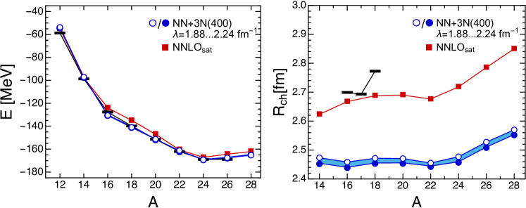
Figure 10: MR-IMSRG(2) ground-state energies and charge radii of the oxygen isotopes for $\text{NNLO}_{\text{sat}}$ and NN+3N(400) at $\lambda=1.88,\ldots,2.24\,\text{fm}^{-1}$ (see text). Black bars indicate experimental data [87, 121].

While chiral NN+3N interactions give a good reproduction of the oxygen ground-state energies, their performance can differ significantly for other observables, as illustrated in Fig. 10. The NN+3N(400) Hamiltonian [77, 65] that was also used in Figs. 8 and 9 underestimates the experimentally known oxygen charge radii by about 10%, and misses the sharp increase for ${}^{18}\mathrm{O}$. The other shown interaction, $\text{NNLO}_{\text{sat}}$ [17] improves the situation significantly, in part because its LECs (cf. Sec. 2) are optimized with a protocol that includes selected many-body data, including the charge radius of ${}^{16}\mathrm{O}$ — however, it also falls short in ${}^{18}\mathrm{O}$ [122].

As we go to heavier nuclei, the NN+3N(400) increasingly overestimates the nuclear binding energy, up to about 1 MeV/nucleon in the light tin isotopes, which are the heaviest nuclei whose ground states we can converge in the MR-IMSRG(2) scheme for this specific input. This overbinding then goes along with an expected underestimation of nuclear charge radii, e.g., for the calcium isotopes shown in Fig. 11. $\text{NNLO}_{\text{sat}}$, on the other hand, is the first chiral NN+3N interaction that gives realistic binding energies and charge radii for ${}^{40}\mathrm{Ca}$ and ${}^{48}\mathrm{Ca}$ at the same time [123, 124]. Unfortunately, it is also a considerably harder interaction than NN+3N(400), and we already encounter convergence problems if we move a few isotopic chains past calcium.

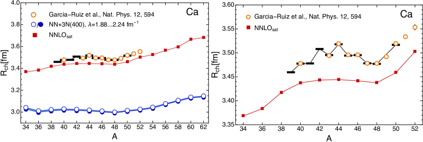
Figure 11: MR-IMSRG(2) charge radii of the calcium isotopes for $\text{NNLO}_{\text{sat}}$ and NN+3N(400) with $\lambda=1.88,\ldots,2.24\,\text{fm}^{-1}$. Note the scale in the zoomed-in second panel. Black bars indicate experimental data [87, 121].

Focusing on the calcium radii shown in the zoomed plot in the right panel of Fig. 11, we see that we do not reproduce the inverted parabolic trend between ${}^{40}\mathrm{Ca}$ and ${}^{48}\mathrm{Ca}$. In traditional nuclear Shell Model/Configuration Interaction (CI) calculations with empirical interactions, this is explained due to configuration mixing of states containing 4p4h (Quadruples in chemistry parlance) and possibly higher excitations [125] that are not included in the MR-IMSRG(2) due to the truncation of the operators at the two-body level, and the use of spherical, particle-number projected HFB vacua as reference states in these calculations. We will discuss this issue in more depth in the next section.

6 Reference States with Static Correlation

As explained in Sec. 4, the IMSRG allows us to control which correlations are built into the reference state and the RG-improved Hamiltonian, respectively. This flexibility offers us an appealing option for addressing the lack of specific features in nuclear charge radii that we described at the end of Sec. 5.

Many-body bases built from a Slater determinant reference and its particle-hole excitations work best for systems with large gaps in the single-particle spectrum, such as closed-shell nuclei. If the gap is small, particle-hole excited basis states can be near-degenerate with the reference determinant, which results in strong configuration mixing. When the mixing involves configurations in which many nucleons are excited simultaneously, we will have static or collective correlations in the wave function, as opposed to dynamic correlations that result from a small number of nucleons only.

Important examples are the emergence of nuclear superfluidity [126] or diverse rotational and vibrational bands in open-shell nuclei (see, e.g., [127]). These phenomena are conveniently described by using the concept of intrinsic wave functions that explicitly break appropriate symmetries of the Hamiltonian. For instance, nuclear superfluidity can be treated to leading-order by introducing quasiparticles that are defined as superpositions of particle and holes [128, 129, 103]. The ground-state of an open-shell nucleus can be expressed as an antisymmetrized product state of these quasiparticles, which can then be optimized variationally — this is precisely the HFB method that was the first step in the generation of references states for the studies of isotopic chains discussed in Sec. 5. The intrinsic HFB wave functions are superpositions of states with different particle numbers, hence we eventually proceeded to restore the symmetry by particle number projection. Such approaches that involve symmetry breaking and subsequent restoration via projection have a long history in nuclear many-body theory [130, 103, 131, 132, 133, 134, 135, 136, 137, 138, 139, 140]).

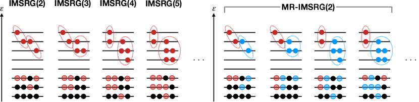
Figure 12: Schematic view of correlations in nuclei. Solid circles indicate nucleons, transparent circles hole states, and dashed ellipses indicate correlations between nucleons. The left panel indicates the IMSRG truncation that would be required to describe the sketched 2p2h (Doubles), 3p3h (Triples), etc. correlations. In the right panel, certain 2p2h as well as all 3p3h and higher correlations (indicated in blue) are built into a correlated wave function that then serves as the reference state for an MR-IMSRG(2) calculation.

The benefit of symmetry breaking and projection methods is that they capture static correlations in a set of simple one-body transition density matrices [103, 140]. Instead of using a Slater determinant reference state and trying to describe static correlations via 3p3h (Triples), 4p4h (Quadruples) and higher excitations of this reference via a high-rank IMSRG evolution (left panel of Fig. 12), we can use a correlated reference state whose irreducible density matrices $\lambda^{(k)}$ we can construct on the fly with little effort, and perform an MR-IMSRG(2) evolution to treat the dynamical correlation on top of this state (right panel of Fig. 12).

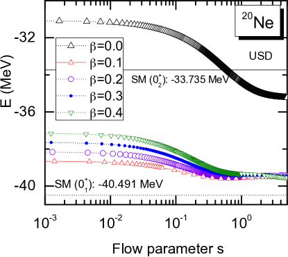
Figure 13: MR-IMSRG(2) energy of ${}^{20}\mathrm{Ne}$, starting from reference states with prolate intrinsic deformations $\beta\geq 0$ that are subsequently projected on angular momentum $J^{\pi}=0^{+}$. These proof-of-principle calculations were performed with the USD Shell Model interaction [141, 142].

As a proof of principle, we show MR-IMSRG(2) calculations for the nucleus ${}^{20}\mathrm{Ne}$ in Fig. 13. Both the proton and neutron shells are open in ${}^{20}\mathrm{Ne}$, which causes the ground-state to develop prolate intrinsic deformation. We obtain reference states by performing HFB calculations with a constraint on the quadrupole moment of the many-body state, and subsequently projecting them on good particle number and angular momentum $J^{\pi}=0^{+}$. The references with prolate deformation ($\beta>0.0$) flow towards the same $0^{+}$ ground state whose energy is close to the result of an exact diagonalization with the empirical USD Hamiltonian [141, 142] we use in our calculation. A spherical reference state ($\beta=0.0$) flows to an excited $0^{+}$ state in the spectrum of ${}^{20}\mathrm{Ne}$ instead.

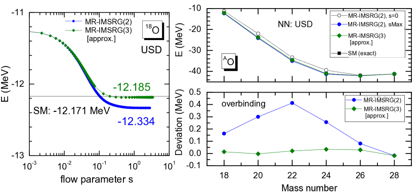
Figure 14: MR-IMSRG(2) and approximate MR-IMSRG(3) ground-state energies of the oxygen isotopes, using the USD Shell Model interaction [141, 142].

The discrepancies between the MR-IMSRG(2) energies for the intrinsically prolate and spherical states and the exact Shell Model results are caused by the truncation of the flow equations at the two-body level. While a full MR-IMSRG(3) calculation would have a computational cost of $\mathcal{O}(N^{9})$, one-step approximations that leverage information from the MR-IMSRG(2) can be implemented at a more manageable $\mathcal{O}(N^{7})$ effort [143], analogous to completely renormalized Coupled Cluster schemes that account for leading Triples excitations [144, 145]. In the left panel of Fig. 14, we perform such an approximate MR-IMSRG(3) calculation for ${}^{18}\mathrm{O}$, and find that we recover the exact diagonalization result[146]. In the right panel, we show that the same improvement is found for all even oxygen isotopes, which is very promising for future applications of the approximate MR-IMSRG(3) in general open-shell nuclei.

7 RG-Improved Hamiltonians: Merging (MR-)IMSRG with Other Many-Body Methods

In the previous sections we have focused on using the (MR-)IMSRG to directly calculate the ground-state energy of nuclei, expressed as the zero-body part of the RG-improved Hamiltonian in the limit $s\to\infty$. We are only realizing a fraction of the power and utility of the (MR-)IMSRG framework in this way: In principle, we have the entire Hamiltonian at our disposal, and not just at the end-point of the flow, but along an entire RG trajectory, which equips us with additional diagnostic power — we recall the variation of the triton ground-state energy with the resolution scale in a free-space SRG, and how we can draw conclusions about missing induced forces from it (see Sec. 3).

In our discussion of Fig. 6, we pointed out that the suppression of the off-diagonal matrix elements that couple the ground state to 2p2h excitations will also eliminate the outermost side diagonals of the Hamiltonian matrix, which implies that it can be beneficial to use the RG-improved Hamiltonian as an input for a secondary many-body calculation. We have explored this idea in several ways:

• With a simple modification of the definition of the off-diagonal Hamiltonian, it is possible to systematically derive effective interactions and operators for valence-space CI calculations, i.e., the traditional interacting Shell Model [95, 110, 111, 147]. This allows us to make use of existing technology to study any nucleus whose low-lying states can be converged in typical Shell Model calculations, explaining the coverage of the nuclear chart we have shown in Fig. 1. it also directly connects Shell Model phenomenology to the underlying chiral interactions — the valence-space diagonalization is merely an approximation to a no-core, large-scale diagonalization. In applications for $sd$-shell nuclei ($8\leq Z\leq 20$), we were able to achieve a surprisingly good agreement with calculations using the gold standard empirical USD interaction [141, 142], which itself has an rms deviation of a mere $\sim 130\,\text{keV}$ for more than 600 energy levels in this region of the nuclear chart.

• The (MR-)IMSRG was recently merged with the No-Core Shell Model (NCSM) into the so-called In-Medium NCSM, in an effort to combine the strengths of the two approaches [148]. A NCSM calculation in a small space provides a correlated reference state for the normal ordering and MR-IMSRG evolution, which enhances the Hamiltonian with dynamical correlation corresponding whose description would otherwise require extremely large NCSM model spaces. For NCSM reference states, the decoupling of the ground-state from excitations is not perfect, hence a secondary small NCSM diagonalization is performed to extract the low-lying eigenvalues and the associated eigenstates. In the IM-NCSM, we make explicit use of the Hamiltonian’s flow-parameter dependence for diagnostic purposes (see Ref. [148] for more details).

• Finally, the ground-state decoupled Hamiltonian can be used as input for Equation-of-Motion (EOM) methods like the well-known Tamm-Dancoff (TDA) and Random Phase Approximations (RPA). TDA and RPA will actually become identical for an IMSRG Hamiltonian, because the ground-state decoupling removes the feedback of RPA correlations into the ground state [149]. EOM calculations are complementary to the CI-based approaches discussed above because they allow us to explore the effects of large single-particle bases, at the cost of limiting the particle rank of the excitation operator for computational efficiency. Thus, they are best suited for the description of dynamical correlations in excited states, although the development of an MR-EOM approach based on correlated reference states is in progress.

The combination of the (MR-)IMSRG with CI/Shell Model techniques allows us to treat both dynamical and static correlation (see Sec. 6), but limits us through the factorial computational scaling of the diagonalization step. As already pointed out by White in Ref. [47], the Density Matrix Renormalization Group (DMRG) can be an appealing and efficient alternative to large-scale CI methods, especially when combined with (MR-)IMSRG decoupling (or Canonical Diagonalization in his choice of words). This idea was pursed by Yanai and co-workers in quantum chemistry [98, 48, 150, 151, 152]), and we are exploring its applications in nuclear physics.

Finally, we are looking ahead at applications of the IMSRG framework to the description of nuclei with cluster structures, and eventually reaction processes. Such structures and processes are most conveniently modeled on spatial lattices, which is why we are working on formulating the IMSRG in that context. Tensor RG methods that generalize the ideas of DMRG to higher dimensions have been very successful in describing correlated systems on spatial lattices could be an ideal complement to the IMSRG (see, e.g., [54, 55, 56]) . Interestingly, these Tensor RGs rely on unitary transformations to disentangle long- and short-range physics that are at least superficially reminiscent of SRG and IMSRG transformations — this certainly merits further investigation.

8 Conclusions and Outlook

In this contribution, we have attempted to illustrate the current reach and capabilities of modern ab initio nuclear structure theory, using the (MR-)IMSRG as a representative example. The discussion is by no means exhaustive, given the rapid rate at which new advances are being introduced. While our focus was on the many-body method, the presented results show that the input NN+3N interactions from chiral EFT are currently the dominant source of uncertainty in our theoretical results, but promising new chiral interactions [17, 66, 8, 9, 5, 153] are now being explored by the nuclear many-body community. The MR-IMSRG will be particularly useful in the community’s efforts to confront these new Hamiltonians with current and forthcoming experimental data for medium-mass and heavy open-shell nuclei.

Work is currently underway to extend the MR-IMSRG framework in several directions, including the coupling to continuum degrees of freedom, and the treatment of intrinsic deformation. The present contribution showed first proof-of-principle results for the latter, implementing the MR-IMSRG transformation with an intrinsically deformed, angular-momentum projected reference state. We plan to extend this work further by using the Generator Coordinate Method to mix multiple projected configurations (see, e.g., [103]).

Motivated by our successes in using the (MR-)IMSRG to construct RG-improved Hamiltonians that can serve as input for the traditional nuclear Shell Model/CI [110, 111, 147], the No-Core Shell Model [148], and EOM methods [149], we seek to integrate the (MR-)IMSRG evolution with further approaches, in particular DMRG, which presents an appealing alternative to costly diagonalization methods for treating static correlations in configuration space. Such a combination of the IMSRG for the Hamiltonian with an entanglement-based RG for wave functions could also offer interesting opportunities for describing strongly interacting systems on spatial or spacetime lattices.

References

- [1] Detmold W 2015 Nuclear Physics from Lattice QCD (Springer International Publishing) pp 153–194 ISBN 978-3-319-08022-2 URL http://dx.doi.org/10.1007/978-3-319-08022-2_5
- [2] Epelbaum E, Hammer H W and Meißner U G 2009 Rev. Mod. Phys. 81(4) 1773–1825 URL http://link.aps.org/doi/10.1103/RevModPhys.81.1773
- [3] Machleidt R and Entem D 2011 Phys. Rept. 503 1 – 75 ISSN 0370-1573 URL http://www.sciencedirect.com/science/article/pii/S0370157311000457
- [4] Epelbaum E, Krebs H and Meißner U G 2015 Phys. Rev. Lett. 115(12) 122301 URL http://link.aps.org/doi/10.1103/PhysRevLett.115.122301
- [5] Entem D R, Kaiser N, Machleidt R and Nosyk Y 2015 Phys. Rev. C 91(1) 014002 URL http://link.aps.org/doi/10.1103/PhysRevC.91.014002
- [6] Machleidt R and Sammarruca F 2016 Physica Scripta 91 083007 URL http://stacks.iop.org/1402-4896/91/i=8/a=083007
- [7] Gezerlis A, Tews I, Epelbaum E, Freunek M, Gandolfi S, Hebeler K, Nogga A and Schwenk A 2014 Phys. Rev. C 90(5) 054323 URL http://link.aps.org/doi/10.1103/PhysRevC.90.054323
- [8] Lynn J E, Tews I, Carlson J, Gandolfi S, Gezerlis A, Schmidt K E and Schwenk A 2016 Phys. Rev. Lett. 116(6) 062501 URL http://link.aps.org/doi/10.1103/PhysRevLett.116.062501
- [9] Lynn J E, Tews I, Carlson J, Gandolfi S, Gezerlis A, Schmidt K E and Schwenk A 2017 Phys. Rev. C 96(5) 054007 URL https://link.aps.org/doi/10.1103/PhysRevC.96.054007
- [10] Pastore S, Girlanda L, Schiavilla R, Viviani M and Wiringa R B 2009 Phys. Rev. C 80(3) 034004 URL http://link.aps.org/doi/10.1103/PhysRevC.80.034004
- [11] Pastore S, Girlanda L, Schiavilla R and Viviani M 2011 Phys. Rev. C 84(2) 024001 URL http://link.aps.org/doi/10.1103/PhysRevC.84.024001
- [12] Piarulli M, Girlanda L, Marcucci L E, Pastore S, Schiavilla R and Viviani M 2013 Phys. Rev. C 87(1) 014006 URL http://link.aps.org/doi/10.1103/PhysRevC.87.014006
- [13] Kölling S, Epelbaum E, Krebs H and Meißner U G 2009 Phys. Rev. C 80(4) 045502 URL http://link.aps.org/doi/10.1103/PhysRevC.80.045502
- [14] Kölling S, Epelbaum E, Krebs H and Meißner U G 2011 Phys. Rev. C 84(5) 054008 URL http://link.aps.org/doi/10.1103/PhysRevC.84.054008
- [15] Barnea N, Contessi L, Gazit D, Pederiva F and van Kolck U 2015 Phys. Rev. Lett. 114(5) 052501 URL https://link.aps.org/doi/10.1103/PhysRevLett.114.052501
- [16] Contessi L, Lovato A, Pederiva F, Roggero A, Kirscher J and van Kolck U 2017 Physics Letters B 772 839–848 URL http://www.sciencedirect.com/science/article/pii/S0370269317306044
- [17] Ekström A, Jansen G R, Wendt K A, Hagen G, Papenbrock T, Carlsson B D, Forssén C, Hjorth-Jensen M, Navrátil P and Nazarewicz W 2015 Phys. Rev. C 91(5) 051301 URL http://link.aps.org/doi/10.1103/PhysRevC.91.051301
- [18] Shirokov A M, Shin I J, Kim Y, Sosonkina M, Maris P and Vary J P 2016 Physics Letters B 761 87–91 URL http://www.sciencedirect.com/science/article/pii/S0370269316304269
- [19] Lepage G P 1989 (Preprint hep-ph/0506330)
- [20] Lepage G P 1997 (Preprint nucl-th/9706029)
- [21] Bogner S K, Kuo T T S and Schwenk A 2003 Phys. Rept. 386 1–27 (Preprint nucl-th/0305035)
- [22] Bogner S K, Furnstahl R J and Perry R J 2007 Phys. Rev. C 75 061001(R) (Preprint nucl-th/0611045)
- [23] Bogner S K, Furnstahl R J and Schwenk A 2010 Prog. Part. Nucl. Phys. 65 94–147 (Preprint 0912.3688)
- [24] Furnstahl R J and Hebeler K 2013 Rept. Prog. Phys. 76 126301 URL http://stacks.iop.org/0034-4885/76/i=12/a=126301
- [25] Glazek S D and Wilson K G 1993 Phys. Rev. D 48 5863–5872
- [26] Wegner F 1994 Ann. Phys. (Leipzig) 3 77
- [27] Bogner S K, Furnstahl R J, Ramanan S and Schwenk A 2006 Nucl. Phys. A 773 203–220 URL http://www.sciencedirect.com/science/article/B6TVB-4K4WG34-2/2/218ed5e2e993065d0432f1ffeafdc50e
- [28] Roth R and Langhammer J 2010 Phys. Lett. B 683 272 – 277 ISSN 0370-2693 URL http://www.sciencedirect.com/science/article/pii/S037026930901507X
- [29] Tichai A, Langhammer J, Binder S and Roth R 2016 Physics Letters B 756 283–288 URL http://www.sciencedirect.com/science/article/pii/S0370269316002008
- [30] Barrett B R, Navrátil P and Vary J P 2013 Prog. Part. Nucl. Phys. 69 131 – 181 ISSN 0146-6410 URL http://www.sciencedirect.com/science/article/pii/S0146641012001184
- [31] Jurgenson E D, Maris P, Furnstahl R J, Navrátil P, Ormand W E and Vary J P 2013 Phys. Rev. C 87(5) 054312 URL http://link.aps.org/doi/10.1103/PhysRevC.87.054312
- [32] Hergert H, Binder S, Calci A, Langhammer J and Roth R 2013 Phys. Rev. Lett. 110(24) 242501 URL http://link.aps.org/doi/10.1103/PhysRevLett.110.242501
- [33] Roth R, Calci A, Langhammer J and Binder S 2014 Phys. Rev. C 90(2) 024325 URL http://link.aps.org/doi/10.1103/PhysRevC.90.024325
- [34] Binder S, Langhammer J, Calci A and Roth R 2014 Phys. Lett. B 736 119 – 123 ISSN 0370-2693 URL http://www.sciencedirect.com/science/article/pii/S0370269314004961
- [35] Hagen G, Papenbrock T, Hjorth-Jensen M and Dean D J 2014 Rept. Prog. Phys. 77 096302 URL http://stacks.iop.org/0034-4885/77/i=9/a=096302
- [36] Hagen G, Hjorth-Jensen M, Jansen G R and Papenbrock T 2016 Phys. Scripta 91 063006 URL http://stacks.iop.org/1402-4896/91/i=6/a=063006
- [37] Hergert H 2017 Phys. Scripta 92 023002 URL http://stacks.iop.org/1402-4896/92/i=2/a=023002
- [38] Tsukiyama K, Bogner S K and Schwenk A 2011 Phys. Rev. Lett. 106 222502
- [39] Hergert H, Bogner S K, Binder S, Calci A, Langhammer J, Roth R and Schwenk A 2013 Phys. Rev. C 87(3) 034307 URL http://link.aps.org/doi/10.1103/PhysRevC.87.034307
- [40] Hergert H, Bogner S K, Morris T D, Schwenk A and Tsukiyama K 2016 Physics Reports 621 165–222 URL http://www.sciencedirect.com/science/article/pii/S0370157315005414
- [41] Kehrein S 2006 The Flow Equation Approach to Many-Particle Systems (Springer Tracts in Modern Physics vol 237) (Springer Berlin / Heidelberg)
- [42] Heidbrink C and Uhrig G 2002 Eur. Phys. J. B 30(4) 443–459 ISSN 1434-6028 10.1140/epjb/e2002-00401-9 URL http://dx.doi.org/10.1140/epjb/e2002-00401-9
- [43] Drescher N A, Fischer T and Uhrig G S 2011 Eur. Phys. J. B 79(2) 225–240 ISSN 1434-6028 10.1140/epjb/e2010-10723-6 URL http://dx.doi.org/10.1140/epjb/e2010-10723-6
- [44] Krull H, Drescher N A and Uhrig G S 2012 Phys. Rev. B 86(12) 125113 URL http://link.aps.org/doi/10.1103/PhysRevB.86.125113
- [45] Fauseweh B and Uhrig G S 2013 Phys. Rev. B 87(18) 184406 URL http://link.aps.org/doi/10.1103/PhysRevB.87.184406
- [46] Krones J and Uhrig G S 2015 Phys. Rev. B 91(12) 125102 URL http://link.aps.org/doi/10.1103/PhysRevB.91.125102
- [47] White S R 2002 J. Chem. Phys. 117 7472–7482 ISSN 00219606 URL http://dx.doi.org/doi/10.1063/1.1508370
- [48] Yanai T and Chan G K L 2007 J. Chem. Phys. 127 104107 (pages 14) URL http://link.aip.org/link/?JCP/127/104107/1
- [49] Nakatsuji H 1976 Phys. Rev. A 14(1) 41–50 URL http://link.aps.org/doi/10.1103/PhysRevA.14.41
- [50] Mukherjee D and Kutzelnigg W 2001 J. Chem. Phys. 114 2047–2061 URL http://link.aip.org/link/?JCP/114/2047/1
- [51] Mazziotti D A 2006 Phys. Rev. Lett. 97(14) 143002 URL http://link.aps.org/doi/10.1103/PhysRevLett.97.143002
- [52] Evangelista F A 2014 J. Chem. Phys. 141 054109 URL http://scitation.aip.org/content/aip/journal/jcp/141/5/10.1063/1.4890660
- [53] White S R 1992 Phys. Rev. Lett. 69(19) 2863–2866 URL https://link.aps.org/doi/10.1103/PhysRevLett.69.2863
- [54] Vidal G 2007 Phys. Rev. Lett. 99(22) 220405 URL https://link.aps.org/doi/10.1103/PhysRevLett.99.220405
- [55] Evenbly G and Vidal G 2009 Phys. Rev. Lett. 102(18) 180406 URL https://link.aps.org/doi/10.1103/PhysRevLett.102.180406
- [56] Evenbly G and Vidal G 2015 Phys. Rev. Lett. 115(18) 180405 URL https://link.aps.org/doi/10.1103/PhysRevLett.115.180405
- [57] Gross D J and Wilczek F 1973 Phys. Rev. Lett. 30(26) 1343–1346 URL http://link.aps.org/doi/10.1103/PhysRevLett.30.1343
- [58] Politzer H D 1973 Phys. Rev. Lett. 30(26) 1346–1349 URL http://link.aps.org/doi/10.1103/PhysRevLett.30.1346
- [59] Weinberg S 1991 Nuclear Physics B 363 3–18 URL http://www.sciencedirect.com/science/article/pii/055032139190231L
- [60] Weinberg S 1996 The Quantum Theory of Fields, Vol. II. Modern Applications 2nd ed (UK: Cambridge University Press)
- [61] Epelbaum E 2010 (Preprint 1001.3229)
- [62] Heisenberg W 1932 Zeitschrift für Physik 77 1–11 URL https://doi.org/10.1007/BF01342433
- [63] Goldstone J 1961 Il Nuovo Cimento (1955-1965) 19 154–164 URL https://doi.org/10.1007/BF02812722
- [64] Melendez J A, Wesolowski S and Furnstahl R J 2017 Phys. Rev. C 96(2) 024003 URL https://link.aps.org/doi/10.1103/PhysRevC.96.024003
- [65] Gazit D, Quaglioni S and Navrátil P 2009 Phys. Rev. Lett. 103(10) 102502 URL http://link.aps.org/doi/10.1103/PhysRevLett.103.102502
- [66] Reinert P, Krebs H and Epelbaum E 2017 (Preprint 1711.08821)
- [67] Valderrama M P, Sánchez M S, Yang C J, Long B, Carbonell J and van Kolck U 2017 Phys. Rev. C 95(5) 054001 URL https://link.aps.org/doi/10.1103/PhysRevC.95.054001
- [68] Sánchez M S, Yang C J, Long B and van Kolck U 2018 Phys. Rev. C 97(2) 024001 URL https://link.aps.org/doi/10.1103/PhysRevC.97.024001
- [69] Coester F, Cohen S, Day B and Vincent C M 1970 Phys. Rev. C 1(3) 769–776 URL https://link.aps.org/doi/10.1103/PhysRevC.1.769
- [70] Bethe H A 1971 Ann. Rev. Nucl. Sci. 21 93–244 URL http://dx.doi.org/10.1146/annurev.ns.21.120171.000521
- [71] Kuckei J, Montani F, Muther H and Sedrakian A 2003 Nucl. Phys. A 723 32–44 (Preprint nucl-th/0210010)
- [72] Hebeler K, Bogner S K, Furnstahl R J, Nogga A and Schwenk A 2011 Phys. Rev. C 83(3) 031301 URL http://link.aps.org/doi/10.1103/PhysRevC.83.031301
- [73] Hebeler K and Furnstahl R J 2013 Phys. Rev. C 87(3) 031302 URL http://link.aps.org/doi/10.1103/PhysRevC.87.031302
- [74] Wiringa R B, Stoks V G J and Schiavilla R 1995 Phys. Rev. C 51(1) 38–51 URL https://link.aps.org/doi/10.1103/PhysRevC.51.38
- [75] Carlson J, Gandolfi S, Pederiva F, Pieper S C, Schiavilla R, Schmidt K E and Wiringa R B 2015 Rev. Mod. Phys. 87(3) 1067–1118 URL http://link.aps.org/doi/10.1103/RevModPhys.87.1067
- [76] Entem D R and Machleidt R 2003 Phys. Rev. C 68 041001 URL http://link.aps.org/doi/10.1103/PhysRevC.68.041001
- [77] Roth R, Langhammer J, Calci A, Binder S and Navrátil P 2011 Phys. Rev. Lett. 107(7) 072501 URL http://link.aps.org/doi/10.1103/PhysRevLett.107.072501
- [78] Hergert H, Bogner S K, Morris T D, Binder S, Calci A, Langhammer J and Roth R 2014 Phys. Rev. C 90(4) 041302 URL http://link.aps.org/doi/10.1103/PhysRevC.90.041302
- [79] Hagen G, Papenbrock T, Dean D J and Hjorth-Jensen M 2010 Phys. Rev. C 82 034330 URL http://link.aps.org/doi/10.1103/PhysRevC.82.034330
- [80] Roth R, Binder S, Vobig K, Calci A, Langhammer J and Navrátil P 2012 Phys. Rev. Lett. 109(5) 052501 URL http://link.aps.org/doi/10.1103/PhysRevLett.109.052501
- [81] Binder S, Langhammer J, Calci A, Navrátil P and Roth R 2013 Phys. Rev. C 87(2) 021303 URL http://link.aps.org/doi/10.1103/PhysRevC.87.021303
- [82] Somà V, Duguet T and Barbieri C 2011 Phys. Rev. C 84(6) 064317 URL http://link.aps.org/doi/10.1103/PhysRevC.84.064317
- [83] Somà V, Barbieri C and Duguet T 2013 Phys. Rev. C 87(1) 011303 URL http://link.aps.org/doi/10.1103/PhysRevC.87.011303
- [84] Somà V, Barbieri C and Duguet T 2014 Phys. Rev. C 89(2) 024323 URL http://link.aps.org/doi/10.1103/PhysRevC.89.024323
- [85] Somà V, Cipollone A, Barbieri C, Navrátil P and Duguet T 2014 Phys. Rev. C 89(6) 061301 URL http://link.aps.org/doi/10.1103/PhysRevC.89.061301
- [86] Hebeler K 2012 Phys. Rev. C 85(2) 021002 URL http://link.aps.org/doi/10.1103/PhysRevC.85.021002
- [87] Wang M, Audi G, Wapstra A, Kondev F, MacCormick M, Xu X and Pfeiffer B 2012 Chin. Phys. C 36 1603 URL http://stacks.iop.org/1674-1137/36/i=12/a=003
- [88] Jurgenson E D, Navrátil P and Furnstahl R J 2009 Phys. Rev. Lett. 103 082501
- [89] Jurgenson E D, Navrátil P and Furnstahl R J 2011 Phys. Rev. C 83(3) 034301 URL http://link.aps.org/doi/10.1103/PhysRevC.83.034301
- [90] Wendt K A 2013 Advances in the Application of the Similarity Renormalization Group to Strongly Interacting Systems Ph.D. thesis The Ohio State University
- [91] Griesshammer H W 2015 in proceedings of the ”8th International Workshop on Chiral Dynamics” vol PoS(CD15) p 104 (Preprint 1511.00490)
- [92] Kutzelnigg W and Mukherjee D 1997 J. Chem. Phys. 107 432–449 URL http://link.aip.org/link/?JCP/107/432/1
- [93] Kong L, Nooijen M and Mukherjee D 2010 J. Chem. Phys. 132 234107 (pages 8) URL http://link.aip.org/link/?JCP/132/234107/1
- [94] Hagen G, Papenbrock T, Dean D J, Schwenk A, Nogga A, Włoch M and Piecuch P 2007 Phys. Rev. C 76(3) 034302 URL http://link.aps.org/doi/10.1103/PhysRevC.76.034302
- [95] Tsukiyama K, Bogner S K and Schwenk A 2012 Phys. Rev. C 85(6) 061304 URL http://link.aps.org/doi/10.1103/PhysRevC.85.061304
- [96] Morris T D, Parzuchowski N M and Bogner S K 2015 Phys. Rev. C 92(3) 034331 URL http://link.aps.org/doi/10.1103/PhysRevC.92.034331
- [97] Shavitt I and Bartlett R J 2009 Many-Body Methods in Chemistry and Physics: MBPT and Coupled-Cluster Theory (Cambridge University Press)
- [98] Yanai T and Chan G K L 2006 J. Chem. Phys. 124 194106 (pages 16) URL http://link.aip.org/link/?JCP/124/194106/1
- [99] Valdemoro C 1987 Theory and Practice of the Spin-Adapted Reduced Hamiltonians (SRH) (Dordrecht: Springer Netherlands) pp 275–288 ISBN 978-94-009-3855-7 URL http://dx.doi.org/10.1007/978-94-009-3855-7_14
- [100] Kutzelnigg W and Mukherjee D 2002 J. Chem. Phys. 116 4787–4801 URL http://link.aip.org/link/?JCP/116/4787/1
- [101] Kutzelnigg W and Mukherjee D 2004 J. Chem. Phys. 120 7340–7349 URL http://link.aip.org/link/?JCP/120/7340/1
- [102] Kutzelnigg W and Mukherjee D 2004 J. Chem. Phys. 120 7350–7368 URL http://link.aip.org/link/?JCP/120/7350/1
- [103] Ring P and Schuck P 1980 The Nuclear Many-Body Problem 1st ed (Springer)
- [104] Cipollone A, Barbieri C and Navrátil P 2013 Phys. Rev. Lett. 111(6) 062501 URL http://link.aps.org/doi/10.1103/PhysRevLett.111.062501
- [105] Cipollone A, Barbieri C and Navrátil P 2015 Phys. Rev. C 92(1) 014306 URL http://link.aps.org/doi/10.1103/PhysRevC.92.014306
- [106] Otsuka T, Suzuki T, Holt J D, Schwenk A and Akaishi Y 2010 Phys. Rev. Lett. 105(3) 032501 URL http://link.aps.org/doi/10.1103/PhysRevLett.105.032501
- [107] Hagen G, Hjorth-Jensen M, Jansen G R, Machleidt R and Papenbrock T 2012 Phys. Rev. Lett. 108(24) 242501 URL http://link.aps.org/doi/10.1103/PhysRevLett.108.242501
- [108] Epelbaum E, Krebs H, Lähde T A, Lee D, Meißner U G and Rupak G 2014 Phys. Rev. Lett. 112(10) 102501 URL http://link.aps.org/doi/10.1103/PhysRevLett.112.102501
- [109] Holt J, Menéndez J and Schwenk A 2013 Eur. Phys. J. A 49 1–6 ISSN 1434-6001 URL http://dx.doi.org/10.1140/epja/i2013-13039-2
- [110] Bogner S K, Hergert H, Holt J D, Schwenk A, Binder S, Calci A, Langhammer J and Roth R 2014 Phys. Rev. Lett. 113(14) 142501 URL http://link.aps.org/doi/10.1103/PhysRevLett.113.142501
- [111] Stroberg S R, Hergert H, Holt J D, Bogner S K and Schwenk A 2016 Phys. Rev. C 93(5) 051301 URL http://link.aps.org/doi/10.1103/PhysRevC.93.051301
- [112] Hergert H and Roth R 2009 Phys. Rev. C 80(2) 024312 URL http://link.aps.org/doi/10.1103/PhysRevC.80.024312
- [113] Roth R 2009 Phys. Rev. C 79 064324 URL http://link.aps.org/doi/10.1103/PhysRevC.79.064324
- [114] Taube A G and Bartlett R J 2008 J. Chem. Phys. 128 044110 (pages 13) URL http://link.aip.org/link/?JCP/128/044110/1
- [115] Taube A G and Bartlett R J 2008 J. Chem. Phys. 128 044111 (pages 9) URL http://link.aip.org/link/?JCP/128/044111/1
- [116] Lee D 2009 Prog. Part. Nucl. Phys. 63 117 – 154 ISSN 0146-6410 URL http://www.sciencedirect.com/science/article/pii/S014664100800094X
- [117] Hoffman C R, Baumann T, Bazin D, Brown J, Christian G, DeYoung P A, Finck J E, Frank N, Hinnefeld J, Howes R, Mears P, Mosby E, Mosby S, Reith J, Rizzo B, Rogers W F, Peaslee G, Peters W A, Schiller A, Scott M J, Tabor S L, Thoennessen M, Voss P J and Williams T 2008 Phys. Rev. Lett. 100(15) 152502 URL http://link.aps.org/doi/10.1103/PhysRevLett.100.152502
- [118] Caesar C, Simonis J, Adachi T, Aksyutina Y, Alcantara J, Altstadt S, Alvarez-Pol H, Ashwood N, Aumann T, Avdeichikov V, Barr M, Beceiro S, Bemmerer D, Benlliure J, Bertulani C A, Boretzky K, Borge M J G, Burgunder G, Caamano M, Casarejos E, Catford W, Cederkäll J, Chakraborty S, Chartier M, Chulkov L, Cortina-Gil D, Datta Pramanik U, Diaz Fernandez P, Dillmann I, Elekes Z, Enders J, Ershova O, Estrade A, Farinon F, Fraile L M, Freer M, Freudenberger M, Fynbo H O U, Galaviz D, Geissel H, Gernhäuser R, Golubev P, Gonzalez Diaz D, Hagdahl J, Heftrich T, Heil M, Heine M, Heinz A, Henriques A, Holl M, Holt J D, Ickert G, Ignatov A, Jakobsson B, Johansson H T, Jonson B, Kalantar-Nayestanaki N, Kanungo R, Kelic-Heil A, Knöbel R, Kröll T, Krücken R, Kurcewicz J, Labiche M, Langer C, Le Bleis T, Lemmon R, Lepyoshkina O, Lindberg S, Machado J, Marganiec J, Maroussov V, Menéndez J, Mostazo M, Movsesyan A, Najafi A, Nilsson T, Nociforo C, Panin V, Perea A, Pietri S, Plag R, Prochazka A, Rahaman A, Rastrepina G, Reifarth R, Ribeiro G, Ricciardi M V, Rigollet C, Riisager K, Röder M, Rossi D, Sanchez del Rio J, Savran D, Scheit H, Schwenk A, Simon H, Sorlin O, Stoica V, Streicher B, Taylor J, Tengblad O, Terashima S, Thies R, Togano Y, Uberseder E, Van de Walle J, Velho P, Volkov V, Wagner A, Wamers F, Weick H, Weigand M, Wheldon C, Wilson G, Wimmer C, Winfield J S, Woods P, Yakorev D, Zhukov M V, Zilges A, Zoric M and Zuber K (R3B collaboration) 2013 Phys. Rev. C 88(3) 034313 URL http://link.aps.org/doi/10.1103/PhysRevC.88.034313
- [119] Rogers W F, Garrett S, Grovom A, Anthony R E, Aulie A, Barker A, Baumann T, Brett J J, Brown J, Christian G, DeYoung P A, Finck J E, Frank N, Hamann A, Haring-Kaye R A, Hinnefeld J, Howe A R, Islam N T, Jones M D, Kuchera A N, Kwiatkowski J, Lunderberg E M, Luther B, Meyer D A, Mosby S, Palmisano A, Parkhurst R, Peters A, Smith J, Snyder J, Spyrou A, Stephenson S L, Strongman M, Sutherland B, Taylor N E and Thoennessen M 2015 Phys. Rev. C 92(3) 034316 URL http://link.aps.org/doi/10.1103/PhysRevC.92.034316
- [120] Kohley Z, Baumann T, Christian G, DeYoung P A, Finck J E, Frank N, Luther B, Lunderberg E, Jones M, Mosby S, Smith J K, Spyrou A and Thoennessen M 2015 Phys. Rev. C 91(3) 034323 URL http://link.aps.org/doi/10.1103/PhysRevC.91.034323
- [121] Angeli I and Marinova K P 2013 Atomic Data and Nuclear Data Tables 99 69–95 URL http://www.sciencedirect.com/science/article/pii/S0092640X12000265
- [122] Lapoux V, Somà V, Barbieri C, Hergert H, Holt J D and Stroberg S R 2016 Phys. Rev. Lett. 117(5) 052501 URL http://link.aps.org/doi/10.1103/PhysRevLett.117.052501
- [123] Hagen G, Ekström A, Forssén C, Jansen G R, Nazarewicz W, Papenbrock T, Wendt K A, Bacca S, Barnea N, Carlsson B, Drischler C, Hebeler K, Hjorth-Jensen M, Miorelli M, Orlandini G, Schwenk A and Simonis J 2015 Nat. Phys. 12 186 URL http://dx.doi.org/10.1038/nphys3529
- [124] Garcia Ruiz R F, Bissell M L, Blaum K, Ekstrom A, Frommgen N, Hagen G, Hammen M, Hebeler K, Holt J D, Jansen G R, Kowalska M, Kreim K, Nazarewicz W, Neugart R, Neyens G, Nortershauser W, Papenbrock T, Papuga J, Schwenk A, Simonis J, Wendt K A and Yordanov D T 2016 Nat. Phys. 12 594–598 URL http://dx.doi.org/10.1038/nphys3645
- [125] Caurier E, Langanke K, Martínez-Pinedo G, Nowacki F and Vogel P 2001 Physics Letters B 522 240–244 URL http://www.sciencedirect.com/science/article/pii/S0370269301012461
- [126] Dean D J and Hjorth-Jensen M 2003 Rev. Mod. Phys. 75 607–656 (Preprint nucl-th/0210033)
- [127] Bohr A and Mottelson B R 1999 Nuclear Structure, Vol. II: Nuclear Deformations (World Scientific)
- [128] Bardeen J, Cooper L N and Schrieffer J R 1957 Phys. Rev. 106 162
- [129] Bogoliubov N N 1958 Sov. Phys. JETP 7 41
- [130] Peierls R E 1973 Proc. R. Soc. London A 333 157–170 URL http://rspa.royalsocietypublishing.org/content/333/1593/157
- [131] Egido J L and Ring P 1982 Nucl. Phys. A 383 189–204
- [132] Robledo L M 1994 Phys. Rev. C 50(6) 2874–2881 URL http://link.aps.org/doi/10.1103/PhysRevC.50.2874
- [133] Flocard H and Onishi N 1997 Ann. Phys. 254 275
- [134] Sheikh J A and Ring P 2000 Nucl. Phys. A 665 71–91 (Preprint nucl-th/9907065)
- [135] Dobaczewski J, Stoitsov M V, Nazarewicz W and Reinhard P G 2007 Phys. Rev. C 76 054315 (Preprint 0708.0441)
- [136] Bender M, Duguet T and Lacroix D 2009 Phys. Rev. C 79 044319 (Preprint 0809.2045)
- [137] Duguet T, Bender M, Bennaceur K, Lacroix D and Lesinski T 2009 Phys. Rev. C 79 044320 (Preprint 0809.2049)
- [138] Lacroix D, Duguet T and Bender M 2009 Phys. Rev. C 79 044318 (Preprint 0809.2041)
- [139] Lacroix D and Gambacurta D 2012 Phys. Rev. C 86(1) 014306 URL http://link.aps.org/doi/10.1103/PhysRevC.86.014306
- [140] Duguet T 2015 J. Phys. G 42 025107 URL http://stacks.iop.org/0954-3899/42/i=2/a=025107
- [141] Wildenthal B H 1984 Progress in Particle and Nuclear Physics 11 5–51 URL http://www.sciencedirect.com/science/article/pii/0146641084900115
- [142] Brown B A and Wildenthal B H 1988 Annual Review of Nuclear and Particle Science 38 29–66 URL https://doi.org/10.1146/annurev.ns.38.120188.000333
- [143] Morris T D 2016 Systematic Improvements of Ab Initio In-Medium Similarity Renormalization Group Calculations Ph.D. thesis Michigan State University URL http://etd.lib.msu.edu/islandora/object/etd%3A3864
- [144] Piecuch P and Włoch M 2005 J. Chem. Phys. 123 224105 URL http://scitation.aip.org/content/aip/journal/jcp/123/22/10.1063/1.2137318
- [145] Binder S, Piecuch P, Calci A, Langhammer J, Navrátil P and Roth R 2013 Phys. Rev. C 88(5) 054319 URL http://link.aps.org/doi/10.1103/PhysRevC.88.054319
- [146] Brown B A and Richter W A 2006 Phys. Rev. C 74(3) 034315 URL http://link.aps.org/doi/10.1103/PhysRevC.74.034315
- [147] Stroberg S R, Calci A, Hergert H, Holt J D, Bogner S K, Roth R and Schwenk A 2017 Phys. Rev. Lett. 118(3) 032502 URL http://link.aps.org/doi/10.1103/PhysRevLett.118.032502
- [148] Gebrerufael E, Vobig K, Hergert H and Roth R 2017 Phys. Rev. Lett. 118(15) 152503 URL https://link.aps.org/doi/10.1103/PhysRevLett.118.152503
- [149] Parzuchowski N M, Morris T D and Bogner S K 2017 Phys. Rev. C 95(4) 044304 URL https://link.aps.org/doi/10.1103/PhysRevC.95.044304
- [150] Neuscamman E, Yanai T and Chan G K L 2009 J. Chem. Phys. 130 124102 (pages 12) URL http://link.aip.org/link/?JCP/130/124102/1
- [151] Neuscamman E, Yanai T and Chan G K L 2010 J. Chem. Phys. 132 024106 (pages 13) URL http://link.aip.org/link/?JCP/132/024106/1
- [152] Yanai T, Kurashige Y, Neuscamman E and Chan G K L 2010 J. Chem. Phys. 132 024105 (pages 9) URL http://link.aip.org/link/?JCP/132/024105/1
- [153] Entem D R, Kaiser N, Machleidt R and Nosyk Y 2015 Phys. Rev. C 92(6) 064001 URL http://link.aps.org/doi/10.1103/PhysRevC.92.064001