A Unified Framework for Training Neural Networks

Abstract

The lack of mathematical tractability of Deep Neural Networks (DNNs) has hindered progress towards having a unified convergence analysis of training algorithms, in the general setting. We propose a unified optimization framework for training different types of DNNs, and establish its convergence for arbitrary loss, activation, and regularization functions, assumed to be smooth. We show that framework generalizes well-known first- and second-order training methods, and thus allows us to show the convergence of these methods for various DNN architectures and learning tasks, as a special case of our approach. We discuss some of its applications in training various DNN architectures (e.g., feed-forward, convolutional, linear networks), to regression and classification tasks.

1 Introduction

Deep neural networks (DNNs) have been successfully applied to many machine learning and statistical inference problems including speech recognition (Hinton et al., 2012), natural language processing (Collobert and Weston, 2008), and image classification (Krizhevsky et al., 2012). Although the ability of a DNN to approximate any smooth function was known since the 80’s (Cybenko, 1989; Hornik et al., 1989; Barron, 1993), computational approaches to the find optimal weights in the network usually lack theoretical guarantees. The main reason that the involved optimization problems are non-convex (Glorot and Bengio, 2010; Zhang et al., 2017) and NP-hard (Blum and Rivest, 1989). In practice, however, various local search methods, e.g., stochastic gradient descent and back propagation (BP) (LeCun et al., 1998) show excellent training performance (Kingma and Ba, 2014), though their success is not very well understood.

Related Work: Mei et al. (2016) and Hazan et al. (2015) studied the convergence of the local search algorithms to train a neural network with no hidden layer, where the associated optimization problem has a single minimizer. Tian (2017) and Zhong et al. (2017) consider a two-layer neural network with Gaussian inputs under specific assumptions on the weights and number of hidden layers, thus making the resulting loss function convex in a small neighborhood around the global solution. Deep linear networks (i.e., DNNs with identity activation functions) have also gained much attention lately, due to their analytical tractability (Yun et al., 2017). Moreover, increasing the number of hidden layers in such networks does not result in ’bad’ local optima (Lu and Kawaguchi, 2017). Recently,Yun et al. (2017) derived global optimality conditions for deep linear networks. Other approaches for training DNNs, using ADMM, were explored but their convergence remains unknown  (Taylor et al., 2016). Lorenzo and Scardapane (2016) studied distributed training via successive convex approximations of the loss (in a single-layer neural network), focusing on communication-related aspects.

While these works provide promising initial analytical results for training DNNs, they occupy a rather narrow slice in the large DNN training literature. As these methods/results are applicable to specific scenarios, we still lack a comprehensive framework for analyzing the convergence of these methods (as opposed to a mere test and try approach), in a general DNN training setup. This issue is of paramount importance.

Our focus in this work is to develop a general framework for DNN training, using variants of Block-Coordinate Descent (BCD) methods, whereby we split-up a non-convex (coupled) optimization problem into a series of subproblems (one per block of variables/coordinates). However, strong convexity of each subproblem is a necessary condition to ensure convergence (Razaviyayn et al., 2012) - an assumption that rarely holds in general DNN training problems. We remedy the problem by leveraging extensions of BCD methods, namely Block-Successive Upperbound Minimization (BSUM), where the non-convex subproblem is approximated with a carefully constructed convex upperbound (Razaviyayn et al., 2012). We thus devise a general training method, applicable to a wide range of DNNs and learning tasks. Similar ideas on the use of surrogate functions have appeared in the BCD literature (Mairal, 2013). A BCD training algorithm was recently proposed by Zhang and Brand (2017), assuming convex loss functions, Tikhonov regularization and ReLU activation function. In that sense, our algorithm generalizes these results as it makes minimal assumptions on the loss, activation, and regularization functions.

Contributions: We adopt in this paper a general DNN training setting, which encompasses several architectures (feed-forward, convolutional, linear, etc.), and assumes arbitrary (yet smooth) loss and activation functions. We propose a new optimization framework offering provable convergence guarantees, and establish convergence of several algorithms under it, in this general setting. We show that our algorithm can recover many existing training algorithms as special cases, and give sufficient conditions for convergence of these approaches, for general training problems. Additionally, we identity choices of loss and activations functions, which result in convex subproblems where standard BCD methods may be used. We also highlight applications of the proposed framework for general learning tasks (regression, classification), and various DNN architectures (feed-forward, convolutional, linear). We underline that this initial investigation is primarily centered around algorithms resulting from first- and second-order upperbounds, under our proposed framework. Future investigations of other upperbounds, and the resulting algorithms are quite promising.

We present the model and problem formulation in Section 2, the proposed algorithm in Section 3, explore several choices for the upperbound in Section 4, and discuss some applications in training DNNs in Section 5. Due to space limitations, we have moved all the proofs and extra discussions to the appendix.

Notation: We use bold upper-case letters to denote matrices, bold lower-case letters to denote vectors, and calligraphic letters to denote sets. For a given matrix $A$, $\|\boldsymbol{A}\|_{F}$ its Frobenius norm, and $\mbox{\boldmath$A$}^{T}$ its transpose. $\mbox{\boldmath$I$}_{n}$ denotes the $n\times n$ identity matrix, ${\mathbb{B}}$ the binary set, ${\mathbb{R}}^{n}$ is the $n$-dimensional Euclidean space, and $\{n\}$ the set of natural numbers from $1$ to $n$.

2 System Model

We consider a batch training method with $N$ samples, ${\mathcal{T}}=\{(\mbox{\boldmath$x$}_{n},\mbox{\boldmath$y$}_{n})\}_{n=1}^{N}$, where $\mbox{\boldmath$x$}_{n}\in{\mathbb{R}}^{d_{0}}$ and $\mbox{\boldmath$y$}_{n}\in{\mathbb{R}}^{d_{J}}$ denote the input and output of sample $n\in\{N\}$. We let $\mbox{\boldmath$Y$}=[\mbox{\boldmath$y$}_{1},\cdots,\mbox{\boldmath$y$}_{N}]$ , and $\mbox{\boldmath$X$}=[\mbox{\boldmath$x$}_{1},\cdots,\mbox{\boldmath$x$}_{N}]$. We model the input-output mapping by a DNN with $J$ layers as follows:

$$\mbox{\boldmath$Z$}_{0}\rightarrow\boxed{\mbox{\boldmath$W$}_{1}}\rightarrow\boxed{\mbox{\boldmath$\Sigma$}_{1}}\rightarrow\underbrace{\mbox{\boldmath$Z$}_{1}}_{\mbox{\boldmath$\Sigma$}_{1}(\mbox{\boldmath$W$}_{1}\mbox{\boldmath$Z$}_{0})}\rightarrow\boxed{\mbox{\boldmath$W$}_{2}}\rightarrow\boxed{\mbox{\boldmath$\Sigma$}_{2}}\rightarrow\underbrace{\mbox{\boldmath$Z$}_{2}}_{\mbox{\boldmath$\Sigma$}_{2}(\mbox{\boldmath$W$}_{2}\mbox{\boldmath$Z$}_{1})}\rightarrow\cdots\underbrace{\mbox{\boldmath$Z$}_{J}}_{\mbox{\boldmath$\Sigma$}_{J}(\mbox{\boldmath$W$}_{J}\mbox{\boldmath$Z$}_{J-1})}$$ (1)

Note that $\mbox{\boldmath$W$}_{j}\in{\mathcal{W}}_{j}\subseteq{\mathbb{R}}^{d_{j}\times d_{j-1}}$ is the matrix of weights connecting layer $j$ to the previous one (dropping the bias without loss in generality), where ${\mathcal{W}}_{j}$ denotes a closed convex set of feasible weights for $\mbox{\boldmath$W$}_{j}$. Moreover, $\mbox{\boldmath$Z$}_{j}\in{\mathbb{R}}^{d_{j}\times N}$ is the batch output of layer $j$, $\mbox{\boldmath$Z$}_{0}\in{\mathbb{R}}^{d_{0}\times N}$ denotes the batch input of the network, and $\mbox{\boldmath$Z$}_{J}\in{\mathbb{R}}^{d_{J}\times N}$ is its output. $\mbox{\boldmath$\Sigma$}_{j}(\mbox{\boldmath$U$}):{\mathbb{R}}^{d_{j}\times N}\rightarrow{\mathbb{R}}^{d_{j}\times N}$ is the matrix of non-linear activation functions for layer $j$. Thus, the operation of layer $j$ is modeled as, $\mbox{\boldmath$Z$}_{j}=\mbox{\boldmath$\Sigma$}_{j}(\mbox{\boldmath$W$}_{j}\mbox{\boldmath$Z$}_{j-1}),~{}j\in\{J\}$. Moreover, we denote by $\mbox{\boldmath$H$}(\mbox{\boldmath$Z$}_{0}):{\mathbb{R}}^{d_{0}\times N}\rightarrow{\mathbb{R}}^{d_{J}\times N}$ the (matrix-valued) mapping representing the entire network, $\mbox{\boldmath$H$}(\mbox{\boldmath$Z$}_{0})\triangleq~{}\mbox{\boldmath$\Sigma$}_{J}\left(\mbox{\boldmath$W$}_{J}\cdots\mbox{\boldmath$\Sigma$}_{2}(\mbox{\boldmath$W$}_{2}~{}\mbox{\boldmath$\Sigma$}_{1}(\mbox{\boldmath$W$}_{1}\mbox{\boldmath$Z$}_{0}))\right).$

2.1 Problem Formulation

We adopt a general DNN training setting (see Section 1), by minimizing a regularized loss function $f$, which comprises of a loss function $\ell$ (i.e., a distance measure between inputs and outputs) and a regularization function $r_{j}$ for layer $j$ (to prevent overfitting). Formally,

$$f(\overline{{\mbox{\boldmath$W$}}})=\ell\left(\overline{\mbox{\boldmath$W$}},\mbox{\boldmath$H$}(\mbox{\boldmath$X$}),\mbox{\boldmath$Y$}\right)+\sum_{j=1}^{J}r_{j}(\mbox{\boldmath$W$}_{j}) \triangleq\ell(\overline{{\mbox{\boldmath$W$}}})+\sum_{j=1}^{J}r_{j}(\mbox{\boldmath$W$}_{j})~{},$$ (2)

where $\overline{{\mbox{\boldmath$W$}}}=\{\mbox{\boldmath$W$}_{1},\cdots,\mbox{\boldmath$W$}_{J}\}$ is the set of all weights, and $r_{j}(\mbox{\boldmath$W$}_{j}):{\mathbb{R}}^{d_{j}\times d_{j-1}}\rightarrow{\mathbb{R}}$.

Assumption 1

. The loss function, $\ell(\mbox{\boldmath$W$}_{1},\cdots,\mbox{\boldmath$W$}_{J}):{\mathbb{R}}^{d_{1}\times d_{0}}\times\cdots\times{\mathbb{R}}^{d_{J}\times d_{J-1}}\rightarrow{\mathbb{R}}$ is differentiable and Lipschitz continuous. The regularization function, $r_{j}(\mbox{\boldmath$W$}_{j}):{\mathbb{R}}^{d_{j}\times d_{j-1}}\rightarrow{\mathbb{R}}$ is assumed to be differentiable and strongly convex, with constant $\lambda_{j}>0$. Extensions to non-smooth regularization are discussed Appendix A.6.

Assumption 2

. $\mbox{\boldmath$\Sigma$}_{j}(\mbox{\boldmath$U$}):{\mathbb{R}}^{d_{j}\times N}\rightarrow{\mathbb{R}}^{d_{j}\times N}$ is the non-linear activation function for layer $j$ (in matrix form). We assume $\mbox{\boldmath$\Sigma$}_{j}(\mbox{\boldmath$U$})$ to be differentiable in $U$ (though not necessarily convex) and satisfying the bounded-input bounded-output property.

Note that such assumptions are quite prevalent in DNN training literature. With that in mind, we find the optimal weights of the networks by formulating an empirical risk minimization problem as:

$$(P)\begin{cases}\underset{\overline{\boldsymbol{W}}\in{\mathcal{W}}}{\min}~{}f(\overline{{\mbox{\boldmath$W$}}})=\ell(\overline{{\mbox{\boldmath$W$}}})+\sum_{j=1}^{J}r_{j}(\mbox{\boldmath$W$}_{j}),\end{cases}$$ (3)

where ${\mathcal{W}}\triangleq\Pi_{j=1}^{J}{\mathcal{W}}_{j}$, and each ${\mathcal{W}}_{j}$ is a closed convex set. As seen from the above model, this formulation is quite generic: $\ell$ and $r_{j}$ can model several DDN regression and classification problems, and various architectures (modeled by ${\mathcal{W}}$). In general, $f(\overline{{\mbox{\boldmath$W$}}})$ is not jointly convex in the weights due to the apparent coupling among the variables, and the non-linear activation functions. Naturally, the coupling also motivates a BCD approach.

3 Proposed Approach

BCD methods operate by optimizing a single block of variables/coordinates during each iteration, assuming all remaining blocks are fixed. At iteration $k$, blocks $\mbox{\boldmath$W$}_{1},...,\mbox{\boldmath$W$}_{j-1},\mbox{\boldmath$W$}_{j+1},\cdots,\mbox{\boldmath$W$}_{J}$ are fixed, and block $\mbox{\boldmath$W$}_{j}$ is updated to minimize:

$$f_{j}(\mbox{\boldmath$W$}_{j};\mbox{\boldmath$W$}_{-j}^{(k)})\triangleq\ell(\mbox{\boldmath$W$}_{1}^{(k)},\cdots,\mbox{\boldmath$W$}_{j-1}^{(k)},\mbox{\boldmath$W$}_{j},\mbox{\boldmath$W$}_{j+1}^{(k)},\cdots,\mbox{\boldmath$W$}_{J}^{(k)})+r_{j}(\mbox{\boldmath$W$}_{j})~{}.$$ (4)

In the above, superscript ${(k)}$ is the iteration number, and $\mbox{\boldmath$W$}_{-j}^{(k)}=\{\mbox{\boldmath$W$}_{1}^{(k)},\cdots,\mbox{\boldmath$W$}_{j-1}^{(k)},\mbox{\boldmath$W$}_{j+1}^{(k)},\cdots,\mbox{\boldmath$W$}_{J}^{(k)}\}$ denotes the set of all blocks except block $j$, at iteration $k$. While many choices are possible for the update order of the blocks, we adopt the cyclic update rule, where $k$ satisfies $j=k\mod J$, to simplify the presentation. Thus, BCD results in the the following subproblem, at iteration $k$

$$(Q)\begin{cases}\underset{\boldsymbol{W}_{j}\in{\mathcal{W}}_{j}}{\textup{argmin}}~{}f_{j}(\mbox{\boldmath$W$}_{j};\mbox{\boldmath$W$}_{-j}^{(k)}),~{}k=1,2,\cdots\end{cases}$$ (5)

Recall that $f_{j}(\mbox{\boldmath$W$}_{j};\mbox{\boldmath$W$}_{-j}^{(k)})$ denotes the regularized loss, when ‘looking’ only at $\mbox{\boldmath$W$}_{j}$. Note further that $f_{j}(\mbox{\boldmath$W$}_{j};\mbox{\boldmath$W$}_{-j}^{(k)})$ is a composition of non-linear activation functions, followed by $\ell$. Since the activation and the loss function are assumed to be differentiable, then $f_{j}(\mbox{\boldmath$W$}_{j};\mbox{\boldmath$W$}_{-j}^{(k)})$ is differentiable - though not necessarily convex. In general, $(Q)$ is not a convex problem, implying that standard BCD methods are not applicable (convergence cannot be guaranteed). Instead, we leverage recent methods such as, Inexact Flexible Parallel Descent (Facchinei et al., 2014) and Block-Successive Upperbound Minimization (BSUM) (Razaviyayn et al., 2012) where $(Q)$ is solved via a series of carefully designed convex upperbounds on $f_{j}(\mbox{\boldmath$W$}_{j};\mbox{\boldmath$W$}_{-j}^{(k)})$.

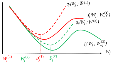
Figure 1: Illustration of Proposed Approach for $\mbox{\boldmath$W$}_{j}$ (2 iterations, $k=1$ in red, $k=2$ in green). Given $\mbox{\boldmath$W$}_{j}^{(1)}$, $g_{j}(\mbox{\boldmath$W$}_{j};\overline{{\mbox{\boldmath$W$}}}^{(k)})$ is an upperbound for $f_{j}(\mbox{\boldmath$W$}_{j};\mbox{\boldmath$W$}_{-j}^{(1)})$. The descent direction $\mbox{\boldmath$D$}_{j}^{(1)}$ is the minimizer of $g_{j}(\mbox{\boldmath$W$}_{j};\overline{{\mbox{\boldmath$W$}}}^{(1)})$. $\mbox{\boldmath$W$}_{j}^{(2)}$ is a convex combination of $\mbox{\boldmath$W$}_{j}^{(1)}$ and $\mbox{\boldmath$D$}_{j}^{(1)}$. $\mbox{\boldmath$W$}_{j}^{(2)}$ is the starting point of second iteration.

Let $g_{j}(\mbox{\boldmath$W$}_{j};\overline{{\mbox{\boldmath$W$}}}^{(k)}):{\mathbb{R}}^{d_{j}}\times{\mathbb{R}}^{d_{j-1}}\rightarrow{\mathbb{R}}$ denote a given convex upperbound of $f_{j}$, at point $\overline{{\mbox{\boldmath$W$}}}^{(k)}$, where $\overline{{\mbox{\boldmath$W$}}}^{(k)}=\{\mbox{\boldmath$W$}_{1}^{(k)},\cdots,\mbox{\boldmath$W$}_{J}^{(k)}\}$. Though many choices are available for the upperbound, they must satisfy some properties (Appendix A.3). Following the method proposed by Facchinei et al. (2014), a surrogate problem for $(Q)$ is posed, where $f_{j}$ is upperbounded by its convex surrogate, $g_{j}$, to find the descent direction $\mbox{\boldmath$D$}_{j}^{(k)}$ for block $\mbox{\boldmath$W$}_{j}^{(k)}$:

$$\tilde{(Q)}:~{}\mbox{\boldmath$D$}_{j}^{(k)}\triangleq\begin{cases}\underset{\boldsymbol{W}_{j}\in{\mathcal{W}}_{j}}{\textup{argmin}}~{}g_{j}(\mbox{\boldmath$W$}_{j};\mbox{\boldmath$W$}_{-j}^{(k)}),~{}k=1,2,\cdots\end{cases}$$ (6)

The strong convexity of $g_{j}(\mbox{\boldmath$W$}_{j};\overline{{\mbox{\boldmath$W$}}}^{(k)})$ and ${\mathcal{W}}_{j}$ (by construction) imply that $\tilde{(Q)}$ is strongly convex, and its solution $\mbox{\boldmath$D$}_{j}^{(k)}$ is unique. Then, $\mbox{\boldmath$W$}_{j}$ is updated as a convex combination of its current value and the descent direction, as follows:

$$\mbox{\boldmath$W$}_{j}^{(k+1)}=(1-\alpha_{j}^{(k)})\mbox{\boldmath$W$}_{j}^{(k)}+\alpha_{j}^{(k)}\mbox{\boldmath$D$}_{j}^{(k)},~{}$$ (7)

where $\alpha_{j}^{(k)}$ is the stepsize satisfying (Facchinei et al., 2014):

$$0\leq\alpha_{j}^{(k)}<1,~{}\lim_{k\rightarrow\infty}\alpha_{j}^{(k)}=0,~{}\sum_{k}\alpha_{j}^{(k)}=\infty,~{}\sum_{k}\alpha_{j}^{(k)^{2}}<\infty,\forall j\in{\mathcal{J}}~{}.$$ (8)

Other choices for $\alpha_{j}^{(k)}$ include small constant (Razaviyayn et al., 2014) or using Armijo’s rule (Facchinei et al., 2014). The approach is illustrated in Figure 1.

3.1 Algorithm Description

Once an upperbound is selected, during each iteration the algorithm updates the descent direction, the stepsize, and the corresponding weights, until convergence; see Algorithm 1. Next, we show the algorithms’ convergence to a stationary point of $(P)$.

Algorithm 1 Training with Alternating Minimization

for $k=1,2,...,$ do

     Set $j=k\mod J$ (for the cyclic update)

     Find descent direction $\mbox{\boldmath$D$}_{j}^{(k)}$ by solving (6)

     Update stepsize $\alpha_{j}^{(k)}$ (satisfying (8))

     Update $\mbox{\boldmath$W$}_{j}^{(k)}$ by solving (7)

end for

Lemma 1 (Convergence of Algorithm 1)

. Let $\{\overline{{\mbox{\boldmath$W$}}}^{(k)}\triangleq(\mbox{\boldmath$W$}_{1}^{(k)},\cdots,\mbox{\boldmath$W$}_{J}^{(k)})\}_{k}$ denote the sequence of iterates generated by the updates in (6) and (7), where $\alpha_{j}^{(k)}$ satisfies the conditions in (8). Then, every limit point of $\{\overline{{\mbox{\boldmath$W$}}}^{(k)}\}$ is a stationary point of $(P)$.

While the proof is based on a stepsize that satisfies (8), convergence still holds in the case of a constant step size (Razaviyayn et al., 2014)[Theorem 1]. $\{f(\overline{{\mbox{\boldmath$W$}}}^{(k)})\}_{k}$, is not necessarily monotonically decreasing: only asymptotic converge of $\{\overline{{\mbox{\boldmath$W$}}}^{(k)}\}$ to a stationary point of $(P)$, as $k\rightarrow\infty$, is guaranteed (Razaviyayn et al., 2014; Facchinei et al., 2014). Note that, Lemma 1 only relies on minimal assumptions (Assumptions 1,2). Thus, convergence holds for almost all loss functions (except the $0/1$ loss), regularization functions, and smooth activation functions (though the result can be extended for piecewise linear functions). Consequently, with a proper choice of upperbounds, we can apply our general algorithm to most DNN learning tasks. Additionally, when $f$ is strongly convex in each of its blocks (see following discussion in Section 4.2.1), the iterations of Algorithm 1 monotonically converge to the stationary point, following standard BCD converge (Tseng, 2001).

4 Choice of Upperbounds

In this section, we explore several choices for the upperbounds $g_{j}$. Each of these choices yields a different cost function for $\tilde{(Q)}$, and consequently, different updates for $\mbox{\boldmath$D$}_{j}^{(k)}$ and $\mbox{\boldmath$W$}_{j}^{(k+1)}$. We focus on the first-order proximal upperbound (next) and proximal upperbound (Section 4.2) in the main text. Derivations on the second-order and linear upperbounds are included in Appendix A.4, and Appendix A.5, respectively. For simplicity, we assume that $\tilde{(Q)}$ is unconstrained.

4.1 First-order Proximal Upperbound

We start with a first-order proximal upperbound,

$$g_{j}(\mbox{\boldmath$W$}_{j};\overline{{\mbox{\boldmath$W$}}}^{(k)}) =f(\overline{{\mbox{\boldmath$W$}}}^{(k)})+{\textup{tr}}\left[\nabla_{\mbox{\boldmath$W$}_{j}}f(\overline{{\mbox{\boldmath$W$}}}^{(k)})^{T}(\mbox{\boldmath$W$}_{j}-\mbox{\boldmath$W$}_{j}^{(k)})\right]+\frac{\gamma_{j}}{2}\|\mbox{\boldmath$W$}_{j}-\mbox{\boldmath$W$}_{j}^{(k)}\|_{F}^{2}~{},$$ (9)

where $\nabla_{\mbox{\boldmath$W$}_{j}}f(\overline{{\mbox{\boldmath$W$}}}^{(k)})=\nabla_{\mbox{\boldmath$W$}_{j}}f(\overline{{\mbox{\boldmath$W$}}})|_{\overline{{\mbox{\boldmath$W$}}}=\overline{{\mbox{\boldmath$W$}}}^{(k)}}$ is the gradient of $f$ with respect to $\mbox{\boldmath$W$}_{j}$ at $\mbox{\boldmath$W$}_{j}^{(k)}$, and $\gamma_{j}>0$ is the Lipschitz constant for $g_{j}(\mbox{\boldmath$W$}_{j};\overline{{\mbox{\boldmath$W$}}}^{(k)})$. Notice that, the upperbound $g_{j}$ is evaluated at point $\overline{{\mbox{\boldmath$W$}}}^{(k)}$, and controlled by the design parameter $\gamma_{j}$. From (9), we can see that $\tilde{(Q)}$ is a strongly convex problem, which can be solved by finding the stationary point of the Lagrangian, resulting in the following updates:

$$\mbox{\boldmath$D$}_{j}^{(k)} =\mbox{\boldmath$W$}_{j}^{(k)}-\gamma_{j}^{-1}\nabla_{\mbox{\boldmath$W$}_{j}}f(\overline{{\mbox{\boldmath$W$}}}^{(k)}),$$

$$\mbox{\boldmath$W$}_{j}^{(k+1)} =\mbox{\boldmath$W$}_{j}^{(k)}-\alpha_{j}^{(k)}\gamma_{j}^{-1}\nabla_{\mbox{\boldmath$W$}_{j}}f(\overline{{\mbox{\boldmath$W$}}}^{(k)}).$$ (10)

The gradient may be computed using the chain rule of calculus; see Appendix B.1. Note that the update in (4.1) is applicable to all loss functions satisfying Assumption 1. In Appendix A.4 we extended the derivations of this section to a second-order upperbound.

4.1.1 Convergence of First- and Second-order methods

Here we can see how the updates resulting from first and second order upperbounds, i.e., (4.1) and (A.4) (Appendix A.4) are generalizations of well-known methods, e.g., back propagation (BP) and its variants, gradient descent, and the Newton-Raphson method.

Special Case 1 (BackPropagation):

Let us first consider the case where we set $\gamma_{j}=1$ in (4.1). Then, the proposed algorithm reduces to the BP method, and $\alpha_{j}^{(k)}$ becomes the learning rate. Recall that different choices of the learning rate have lead to many popular variants of BP, such as constant, decaying, and ADAGRAD. A common drawback of these approaches for choosing the learning rate is the lack of convergence guarantees in most DNN training problems: Therefore it is usually selected via cross validation (Zeiler, 2012). With the proposed algorithm, however, the convergence in Lemma 1 holds for any choice of stepsize satisfying (8).

Corollary 1 (Convergence of BP)

. For any arbitrary smooth loss $f$ (Assumptions 1, 2) the updates of first-order methods in (4.1) converge to a stationary point of $(P)$. This includes BP and many of its variants, e.g., BP with constant but small $\alpha_{j}^{(k)}$, inverse-root $\alpha_{j}^{(k)}=c/\sqrt{k}~{}(c>0)$, Arimijo’s rule, etc., as they satisfy (8). The proof follows directly from Lemma 1.

We underline that convergence of BP for a smooth loss function, for the conditions in (8), was shown by Mangasarian and Solodov (1994)[Theorem 2.1]. However, the result of Corollary 1 also extends to the Newton-Raphson method derived in Appendix A.4.

Special Case 2 (Gradient Descent and Newton-Raphson Method):

Another notable special case of our proposed algorithm is obtained by considering a unit stepsize, i.e., setting $\alpha_{j}^{(k)}=1$ in (4.1). Then, the update for $\mbox{\boldmath$W$}_{j}$ in (4.1) reduces to,

$$\mbox{\boldmath$W$}_{j}^{(k+1)}=\mbox{\boldmath$W$}_{j}^{(k)}-\gamma_{j}^{-1}\nabla_{\mbox{\boldmath$W$}_{j}}f(\overline{{\mbox{\boldmath$W$}}}^{(k)}),$$ (11)

which is the gradient descent, with stepsize $\frac{1}{\gamma_{j}}$. Similarly, when $\alpha_{j}^{(k)}=1$, the update resulting from the second-order upperbound in (A.4) reduces to the Levenberg-Marquardt variant of the Newton-Raphson method (Yu et al., 2011),

$$\mbox{\boldmath$W$}_{j}^{(k+1)}=\mbox{\boldmath$W$}_{j}^{(k)}-\left[\nabla_{\mbox{\boldmath$W$}_{j}}^{2}f(\overline{{\mbox{\boldmath$W$}}}^{(k)})+{\gamma_{j}}\mbox{\boldmath$I$}\right]^{-1}\nabla_{\mbox{\boldmath$W$}_{j}}f(\overline{{\mbox{\boldmath$W$}}}^{(k)}).$$ (12)

Evidently, it is quite desirable to have a convergence proof for these training methods. To our best knowledge, such results are not available in the literature, in the general setting considered here. Note that while setting $\alpha_{j}^{(k)}=1$ violates the stepsize conditions in (8), converge of (11) and (12) follow from the BSUM framework (in the result below).

Lemma 2 (Convergence of Gradient/Newton Methods)

. The updates generated by the gradient method in (11), or Newton’s method in (12), converges to a stationary point of $(P)$.

Discussions: In that sense, our proposed approach complements known training methods (e.g., gradient descent, BP and its variants, Newton), by providing conditions for convergence guarantees. We underline that first- and second-order methods (i.e., BP, gradient descent, Newton’s method) can be interpreted as special cases of the BSUM method (when using first- and second-order upperbounds only), as convex approximations of a (non-convex) loss function around each block.

Practical Issues: The updates resulting from the first-order proximal upperbound require knowledge of the gradient (resp. Hessian) of $f$ with respect to $\mbox{\boldmath$W$}_{j}$: They are similar to BP (resp. LMBFS) methods for training DNNs, in terms of the computational complexity needed to run the algorithms. Moreover, the stochastic training variant (Section 4.1.2) may be used when the training set is too large. Finally, the fact that the algorithm is based on BCD/BSUM methods enables parallel processing, to make algorithm distributed (Lorenzo and Scardapane, 2016).

4.1.2 From Batch to Stochastic Training

In contemporary machine learning tasks, its quite common to deal with large datasets for which the computation of the gradient over all samples is challenging. In such scenarios, we can replace the gradient with its unbiased noisy estimate, and run the following update:

$$\hat{\mbox{\boldmath$W$}}_{j}^{(k+1)} =\hat{\mbox{\boldmath$W$}}_{j}^{(k)}-\alpha_{j}^{(k)}\gamma_{j}^{-1}\widehat{\nabla_{\mbox{\boldmath$W$}_{j}}}f(\overline{{\mbox{\boldmath$W$}}}^{(k)}),~{}$$ (13)

where the stochastic (or mini-batch) gradient, $\widehat{\nabla_{\mbox{\boldmath$W$}_{j}}}f$, is defined in (A.10). Following the results from (Facchinei et al., 2014), if the error is bounded, $\|\hat{\mbox{\boldmath$W$}}_{j}^{(k)}-\mbox{\boldmath$W$}_{j}^{(k)}\|_{F}^{2}\leq\epsilon_{j}^{(k)}$, and $\epsilon_{j}^{(k)}$ decays asymptotically to zero, then the convergence of Algorithm 1 still holds. A complete convergence proof of this stochastic training variation is left for future work.

4.2 Proximal Upperbound:

When $f_{j}(\mbox{\boldmath$W$}_{j};\mbox{\boldmath$W$}_{-j}^{(k)})$ is convex (discussed next), the proximal operator is yet another possible upperbound. Unlike the first-order upperbound, the descent direction is the solution to a proximal-point operator with respect to $\gamma_{j}^{-1}f_{j}$, around $\mbox{\boldmath$W$}_{j}^{(k)}$, as follows:

$$\mbox{\boldmath$D$}_{j}^{(k)}=\textup{prox}_{{\gamma_{j}^{-1}}f_{j}}(\mbox{\boldmath$W$}_{j}^{(k)})=\underset{\boldsymbol{W}_{j}\in{\mathcal{W}}_{j}}{\textup{argmin}}~{}f_{j}(\mbox{\boldmath$W$}_{j};\mbox{\boldmath$W$}_{-j}^{(k)})+\frac{\gamma_{j}}{2}\|\mbox{\boldmath$W$}_{j}-\mbox{\boldmath$W$}_{j}^{(k)}\|_{F}^{2}~{}.$$ (14)

Notice that the update in (14) are a general form of the proximal algorithm by Frerix et al. (2017), developed for the regression problem.

4.2.1 Convexity of $f$ in Each Block

The convexity of $f$ in each of its blocks will impact the algorithm and analytical results. When $f_{j}(\mbox{\boldmath$W$}_{j};\mbox{\boldmath$W$}_{-j}^{(k)})$ is strongly convex (as shown below), then simple BCD methods may be employed instead of upperbounds. In the following, we find conditions on the choice of $\ell$ and $\mbox{\boldmath$\Sigma$}_{j}$, that result in $f_{j}(\mbox{\boldmath$W$}_{j};\mbox{\boldmath$W$}_{-j}^{(k)})$ being convex. From (4), note that $f_{j}$ can be abstracted as:

$$f_{j}(\mbox{\boldmath$W$}_{j};\mbox{\boldmath$W$}_{-j}^{(k)}) =\ell\left[\mbox{\boldmath$\Sigma$}_{J}(\mbox{\boldmath$W$}_{j}^{(k)}\cdots\mbox{\boldmath$\Sigma$}_{j}(\mbox{\boldmath$W$}_{j}\cdots\mbox{\boldmath$\Sigma$}_{1}(\mbox{\boldmath$W$}_{1}^{(k)})))\right]+r_{j}(\mbox{\boldmath$W$}_{j})$$

$$=\ell\left[\mbox{\boldmath$\Sigma$}_{J}(\cdots\mbox{\boldmath$\Sigma$}_{j}(\mbox{\boldmath$W$}_{j}))\right]+r_{j}(\mbox{\boldmath$W$}_{j}).$$ (15)

The second equality follows from noting that composition with an affine function does not alter the convexity/concavity of $f_{j}$ (Boyd and Vandenberghe, 2004)[Chap 3.2.4], implying that the fixed blocks, $\mbox{\boldmath$W$}_{-j}^{(k)}$, may be dropped without altering this analysis: Indeed, $f_{j}$ is a composition of activation functions $\mbox{\boldmath$\Sigma$}_{j},\cdots,\mbox{\boldmath$\Sigma$}_{J}$, followed by $\ell$. We next find two alternate sufficient conditions, that guarantee the strong convexity of $f$ in each of its blocks.

Proposition 1 (Convexity of $f_{j}$)

. $f_{j}(\mbox{\boldmath$W$}_{j};\mbox{\boldmath$W$}_{-j}^{(k)})$ is strongly convex in $\mbox{\boldmath$W$}_{j}$ with constant $\lambda_{j}$, if
C1) $\{\mbox{\boldmath$\Sigma$}_{j}\}_{j=1}^{J}$ is convex and non-decreasing, and $\ell$ is convex and non-decreasing, or
C2) $\{\mbox{\boldmath$\Sigma$}_{j}\}_{j=1}^{J}$ is concave and non-decreasing, and is $\ell$ convex and non-increasing.

While the conditions of C1) are satisfied in many cases (most activation function are convex and non-decreasing), those of C2) are stricter. This result implies that one can engineer convex formulations (via specific choices of $\ell$ and $r_{j}$), where standard BCD methods can be used to solve each subproblem exactly (since $(Q)$ becomes strongly convex). We elaborate on these combinations in Appendix A.1. Similarly, choices of $\ell$ and $\mbox{\boldmath$\Sigma$}_{j}$ that lead to $f_{j}$ being concave in each block are discussed in Appendix A.2.

5 Applications

5.1 Training DNNs

Regression Tasks:

The problem of regression consists of optimizing the non-linear network, to ‘best fit’ a given training set. For a ridge regression, the loss function and regularization are the $l_{2}$-norm  (Bishop, 2006):

$$f(\overline{{\mbox{\boldmath$W$}}})=\frac{1}{N}\|\mbox{\boldmath$Y$}-\mbox{\boldmath$H$}(\mbox{\boldmath$X$})\|_{F}^{2}+\sum_{j}\lambda_{j}\|\mbox{\boldmath$W$}_{j}\|_{F}^{2},~{}\lambda_{j}>0.$$ (16)

Moreover, the feasible set for $\mbox{\boldmath$W$}_{j}$ simply becomes ${\mathcal{W}}_{j}={\mathbb{R}}^{d_{j}\times d_{j-1}}$. Sparse regularization (LASSO) is discussed in Appendix A.6. Essentially, we can run Algorithm 1 for loss functions such as (16), with a guaranteed convergence.

Classification Tasks:

The proposed approach is also applicable to DNN classification tasks, where the regularized cross-entropy loss, in (A.14), is prevalent. Now, we can run Algorithm 1 on  (A.14). Our approach is equally applicable to other classification loss functions, e.g., the regularized squared hinge loss (A.17), and the logistic loss (A.18) (detailed in Appendix B.1).

5.2 Training Various DNN Architectures

Deep Convolutional Neural Networks:

While the methods for regression and classification (Section 5.1) were in the context of classical DNNs, they may be modified to train deep convolutional neural networks. In this setting, the weights for each layer are a Toeplitz matrix, representing the circular convolution operation, where the rows of $\mbox{\boldmath$W$}_{j}$ are taken from the set of $d_{j}\times d_{j-1}$ Toeplitz matrices, ${\mathcal{T}}_{j}$. Moreover, it is known that ${\mathcal{T}}_{j}$ is a closed affine subspace in $\mbox{\boldmath$W$}_{j}$ (Eberle and Maciel, 2003). Thus, $\tilde{(Q)}$ reduces to $\textup{argmin}_{\mbox{\boldmath$W$}_{j}\in{\mathcal{T}}_{j}}~{}g_{j}(\mbox{\boldmath$W$}_{j};\mbox{\boldmath$W$}_{-j}^{(k)})$, where $g_{j}(\mbox{\boldmath$W$}_{j};\mbox{\boldmath$W$}_{-j}^{(k)})$ can be chosen as any of the upperbounds in Section 4, and Appendix A.4. Furthermore, $\tilde{(Q)}$ is strongly convex, since ${\mathcal{T}}_{j}$ is a affine.

Deep Linear Networks:

Deep linear networks are recent attempts at making DNNs (mathematically) tractable, by using identity activation functions; see Section 1. For such system, the model consists of a cascade of linear operators, $\mbox{\boldmath$H$}(\mbox{\boldmath$Z$}_{0})\triangleq~{}(\mbox{\boldmath$W$}_{J}\cdots~{}\mbox{\boldmath$W$}_{1})\mbox{\boldmath$Z$}_{0}$. The proposed method is indeed applicable to training these networks. More specifically, BCD methods are applicable in this case, since $(Q)$ is a strongly convex problem, and can be solved in closed-form.

6 Numerical Results

Simulation setting: We present simple numerical results to validate the various convergence claims, thereby focusing on training rather than test performance. Recall that known methods such as BP with decaying learning rate ($\alpha_{j}^{(k)}=c/\sqrt{k}$) are instances of the proposed method. We also explore other choices of the stepsize , i.e., $\alpha^{(k+1)}=\alpha_{j}^{(k)}(1-t\alpha_{j}^{(k)}),0<t<1$ (Facchinei et al., 2014), and $\alpha_{j}^{(k)}=c/2^{k}$, all of which satisfy the stepsize conditions in (8). We benchmark against other approaches such as, BP with constant learning rate (BP-CLR), and ADAGRAD (Zeiler, 2012). We use the BodyFat regression dataset ($N=252$) for a small DNN (to avoid overfitting) with $J=4$, $d_{0}=13,d_{1}=d_{2}=d_{3}=10$, and $d_{4}=1$. Moreover, the $l_{2}$ loss in (16) and logistic activation function are used.

Figure 2(a) shows the normalized training mean-squared error (MSE), for the various training methods. Moreover, all algorithms converge to a stationary point (as shown in Corollary 1, except for ADAGRAD). Note that the oscillations are still consistent with Lemma 1, as only asymptotic convergence is ensured. We observe that all three variants of the proposed method outperform BP-CLR and ADAGRAG (in terms of convergence rate). An interesting by-product of our framework is the possibility of selecting the best learning algorithm, in terms of convergence rate. Using the same optimization framework, we can implement various algorithms and pick the best, all of which having convergence guarantees.

Recall from Proposition 1 and its related discussions, that we can achieve monotonic convergence when $f$ is strongly convex in each block. The latter is feasible by adopting among others, an exponential loss (given by (A.12)), and a SoftPlus activation. Indeed, condition C1) in Proposition 1 holds in this case, and consequently, monotonic convergence can be shown (using standard BCD convergence), as seen from Figure A.1 in Appendix A.7).

Figure 2(b) additionally shows the training MSE of the stochastic variant, in Section 4.1.2, each with a different batch size $B$. We observe that the performance improves as $B$ increases from $50$ to $200$, as expected. In the last variant, $B$ is increased with the number of iterations (until $B=N$): Thus the variance in the gradient estimate is gradually reduced, allowing for convergence. Note that the results are similar to the convergence behavior of stochastic gradient methods.

(a) Batch training

(b) Mini-batch (stochastic gradient) training

Figure 2: Normalized MSE performance for the proposed schemes and benchmark. “Prop” stands for the proposed approach. “setting 1” is $\alpha^{(k+1)}=\alpha^{(k)}(1-0.99\alpha^{k}),\alpha^{(0)}=1$. In 2(b), the increasing $B$ curve corresponds to $B=\min(k,N)$.

7 Conclusion

In this work, we proposed a framework for training general neural networks and showed its convergence using the BSUM method, for a wide class of DNNs architectures and learning tasks. We showed that updates resulting from first- (resp. second-) order proximal upperbound were in fact generalizations of well-known first-order (resp. Newton) methods. Thus, the proposed method allows us to analyze and show convergence of these methods, for training DNNs. While these connections arise from our investigation of just first- and second-order upperbounds, we wish to explore in the future other upperbounds, which may lead to different algorithms, and further applications (e.g., robustness in learning).

Supplementary Material for

A Unified Framework for Training Neural Networks

Appendix A Additional Results

A.1 Conditions for convex $f_{j}$

Choices of loss and activation functions for which Condition C1) holds (in Proposition 1). Activation functions such as, differentiable variants of the ReLU (leaky, parametric, exponential, scaled exponential, inverse square-root), softplus, Bent identity, and soft exponential. Moreover, the exponential loss in (A.12) is convex and monotonically increasing.

The conditions for C2) holds (in Proposition 1) are stricter, as they are satisfied by log-type activation functions (a subset of soft exponential), and most loss functions such as, smoothed or squared hinge, logistic, and the cross-entropy.

A.2 Conditions for concave $f_{j}$

Note that one may also identify choices of loss and activation function that result in $f$ being concave in each of its blocks: this is case of class for the class of exponentially concave functions, which include the logistic loss in classification [Mahdavi and Jin, 2014], studied by [Mahdavi and Jin, 2014], [Pal and Wong, 2016]. We refer the reader to the survey [Mehta, 2016].

Proposition 2

Consider the case $\{\mbox{\boldmath$\Sigma$}_{j}\}_{j=1}^{J}$ are convex and non-decreasing, $\ell$ is concave a non-increasing, and no regularization is added to $\ell$. Then, $f_{j}$ is concave in each block (the proof follows a similar argument as Proposition 1). In such cases, the gradient can be used as upperbound. Moreover, overfitting can be prevented by including the regularization as a (convex) constraint, ${\mathcal{W}}_{j}=\{r_{j}(\mbox{\boldmath$W$}_{j})\leq\rho_{j}\}$.

A.3 Properties of Upperbounds

Below we formalize the analytical properties of the upperbound s[Facchinei et al., 2014]:

• $g_{j}(\mbox{\boldmath$W$}_{j};\overline{{\mbox{\boldmath$W$}}}^{(k)})$ is continuously differentiable in $\mbox{\boldmath$W$}_{j}$ and has a Lipschitz continuous gradient with constant $\gamma_{j}$.

• $\nabla_{\mbox{\boldmath$W$}_{j}}~{}g_{j}(\mbox{\boldmath$W$}_{j};\overline{{\mbox{\boldmath$W$}}}^{(k)})=\nabla_{\mbox{\boldmath$W$}_{j}}~{}f(\mbox{\boldmath$W$}_{1},\cdots,\mbox{\boldmath$W$}_{J})$

• $g_{j}(\mbox{\boldmath$W$}_{j};\overline{{\mbox{\boldmath$W$}}}^{(k)})$ has a continuous gradient on ${\mathcal{W}}_{j}$

• $g_{j}(\mbox{\boldmath$W$}_{j};\overline{{\mbox{\boldmath$W$}}}^{(k)})$ is strongly convex on ${\mathcal{W}}_{j}$, with Lipschitz constant $\gamma_{j}$

A.4 Second-order Upperbound:

Note that tighter approximations can be done using the Hessian. Naturally, we need to make the added assumptions that $\ell$ and $r_{j}$ are twice differentiable (in this part only). The second-order proximal upperbound is defined as,

$$g_{j}(\mbox{\boldmath$W$}_{j};\overline{{\mbox{\boldmath$W$}}}^{(k)}) =f(\overline{{\mbox{\boldmath$W$}}}^{(k)})+{\textup{tr}}[\nabla_{\mbox{\boldmath$W$}_{j}}f(\overline{{\mbox{\boldmath$W$}}}^{(k)})^{T}(\mbox{\boldmath$W$}_{j}-\mbox{\boldmath$W$}_{j}^{(k)})]+\frac{\gamma_{j}}{2}\|\mbox{\boldmath$W$}_{j}-\mbox{\boldmath$W$}_{j}^{(k)}\|_{F}^{2}$$

$$~{}~{}+\frac{1}{2}{\textup{tr}}[(\mbox{\boldmath$W$}_{j}-\mbox{\boldmath$W$}_{j}^{(k)})^{T}\nabla_{\mbox{\boldmath$W$}_{j}}^{2}f(\overline{{\mbox{\boldmath$W$}}}^{(k)})(\mbox{\boldmath$W$}_{j}-\mbox{\boldmath$W$}_{j}^{(k)})].$$ (A.1)

where $\nabla_{\mbox{\boldmath$W$}_{j}}^{2}f(\overline{{\mbox{\boldmath$W$}}}^{(k)})$ is the Hessian of $f$ with respect to $\mbox{\boldmath$W$}_{j}$, at $\overline{{\mbox{\boldmath$W$}}}^{(k)}$. We can drop the constant invariant terms in the last equation,

$$g_{j}(\mbox{\boldmath$W$}_{j};\overline{{\mbox{\boldmath$W$}}}^{(k)}) ={\textup{tr}}[\nabla_{\mbox{\boldmath$W$}_{j}}f(\overline{{\mbox{\boldmath$W$}}}^{(k)})^{T}\mbox{\boldmath$W$}_{j}]$$

$$~{}~{}+\frac{1}{2}{\textup{tr}}\left[(\mbox{\boldmath$W$}_{j}-\mbox{\boldmath$W$}_{j}^{(k)})^{T}(\nabla_{\mbox{\boldmath$W$}_{j}}^{2}f(\overline{{\mbox{\boldmath$W$}}}^{(k)})+{\gamma_{j}}\mbox{\boldmath$I$})(\mbox{\boldmath$W$}_{j}-\mbox{\boldmath$W$}_{j}^{(k)})\right]$$

With this upperbound $\tilde{(Q)}$ is strongly convex. Using Lagrangian techniques, we derive its solution to obtain the descent direction, and updates:

$$\mbox{\boldmath$D$}_{j}^{(k)} =\mbox{\boldmath$W$}_{j}^{(k)}-[\nabla_{\mbox{\boldmath$W$}_{j}}^{2}f(\overline{{\mbox{\boldmath$W$}}}^{(k)})+{\gamma_{j}}\mbox{\boldmath$I$}]^{-1}\nabla_{\mbox{\boldmath$W$}_{j}}f(\overline{{\mbox{\boldmath$W$}}}^{(k)})$$

$$\mbox{\boldmath$W$}_{j}^{(k+1)} =\mbox{\boldmath$W$}_{j}^{(k)}-\alpha_{j}^{(k)}[\nabla_{\mbox{\boldmath$W$}_{j}}^{2}f(\overline{{\mbox{\boldmath$W$}}}^{(k)})+{\gamma_{j}}\mbox{\boldmath$I$}]^{-1}\nabla_{\mbox{\boldmath$W$}_{j}}f(\overline{{\mbox{\boldmath$W$}}}^{(k)})$$ (A.2)

We recall that the convergence in Corollary 1 still holds for the update in (A.4).

A.5 Linear Upperbound:

Note that when $f_{j}$ is concave in each of its blocks (Appendix A.2), the upperbound in (9) reduces to a linear one, i.e., $g_{j}(\mbox{\boldmath$W$}_{j};\overline{{\mbox{\boldmath$W$}}}^{(k)})=f(\overline{{\mbox{\boldmath$W$}}}^{(k)})+{\textup{tr}}[\nabla_{\mbox{\boldmath$W$}_{j}}f(\overline{{\mbox{\boldmath$W$}}}^{(k)})^{T}(\mbox{\boldmath$W$}_{j}-\mbox{\boldmath$W$}_{j}^{(k)})],$ yields a descent direction $\mbox{\boldmath$D$}_{j}^{(k)}=\nabla_{\mbox{\boldmath$W$}_{j}}f(\overline{{\mbox{\boldmath$W$}}}^{(k)})$, and the following update:

$$\mbox{\boldmath$W$}_{j}^{(k+1)} =(1-\alpha_{j}^{(k)})\mbox{\boldmath$W$}_{j}^{(k)}-\alpha_{j}^{(k)}\nabla_{\mbox{\boldmath$W$}_{j}}f(\overline{{\mbox{\boldmath$W$}}}^{(k)})$$ (A.3)

Following the discussion in Appendix A.2, we highlight the wide class of exponentially concave functions as direct applications of the update in (A.3), for future investigations. Moreover, its convergence follows from Lemma 1.

A.6 Extension to Non-smooth Regularization

Note that the proposed approach can be extended to cases where regularization is non-smooth but convex, i.e., $r_{j}(\mbox{\boldmath$W$}_{j})=\lambda_{j}\|\mbox{\boldmath$W$}_{j}\|_{1}$, where $\|\mbox{\boldmath$A$}\|_{1}=\sum_{(n,m)}|\mbox{\boldmath$A$}_{n,m}|$ . For illustration purposes, we restrict the derivations to the first-order approximations in (9) of the smooth loss . However, the discussion below is applicable to all other upperbounds presented in the work. In the non-smooth regularization case (9) becomes,

$$g_{j}(\mbox{\boldmath$W$}_{j};\mbox{\boldmath$W$}_{-j}^{(k)}) =\ell(\overline{{\mbox{\boldmath$W$}}}^{(k)})+{\textup{tr}}[\nabla_{\mbox{\boldmath$W$}_{j}}\ell(\overline{{\mbox{\boldmath$W$}}}^{(k)})^{T}(\mbox{\boldmath$W$}_{j}-\mbox{\boldmath$W$}_{j}^{(k)})]+\frac{\gamma_{j}}{2}\|\mbox{\boldmath$W$}_{j}-\mbox{\boldmath$W$}_{j}^{(k)}\|_{F}^{2}$$ (A.4)

The descent direction is determined as,

$$\mbox{\boldmath$D$}_{j}^{(k+1)} \triangleq\underset{\mbox{\boldmath$W$}_{j}}{\textup{argmin}}~{}g_{j}(\mbox{\boldmath$W$}_{j};\mbox{\boldmath$W$}_{-j}^{(k)})+r_{j}(\mbox{\boldmath$W$}_{j})=\underset{\mbox{\boldmath$W$}_{j}}{\textup{argmin}}~{}g_{j}(\mbox{\boldmath$W$}_{j};\mbox{\boldmath$W$}_{-j}^{(k)})+\lambda_{j}\|\mbox{\boldmath$W$}_{j}\|_{1}$$

$$=\textup{prox}_{\gamma_{j}^{-1}r_{j}}[\mbox{\boldmath$W$}_{j}^{(k)}-\gamma_{j}^{-1}\nabla_{\mbox{\boldmath$W$}_{j}}~{}g_{j}(\overline{{\mbox{\boldmath$W$}}}^{(k)})]$$ (A.5)

where prox is the proximal operator with respect to $\gamma_{j}^{-1}r_{j}$ , given by the soft thresholding operation [Parikh and Boyd, 2014]:

$$[\textup{prox}_{\frac{1}{\gamma_{j}}r_{j}}(\mbox{\boldmath$A$})]_{n,m}=\begin{cases}[\mbox{\boldmath$A$}]_{n,m}-\frac{\lambda_{j}}{\gamma_{j}}&,~{}[\mbox{\boldmath$A$}]_{n,m}\geq\frac{\lambda_{j}}{\gamma_{j}}\\ 0~{}&,-\frac{\lambda_{j}}{\gamma_{j}}\leq[\mbox{\boldmath$A$}]_{n,m}\leq\frac{\lambda_{j}}{\gamma_{j}}\\ [\mbox{\boldmath$A$}]_{n,m}+\frac{\lambda_{j}}{\gamma_{j}}~{}&,[\mbox{\boldmath$A$}]_{n,m}\leq\frac{\lambda_{j}}{\gamma_{j}}\end{cases}.$$

A.7 Additional Numerical Results

Using the same parametrization of Section 6, we change exponential loss (given by (A.12)), and a SoftPlus activation. The resulting loss is convex in each block of coordinates. Convergence of the various algorithms is shown in Figure A.1.

Figure A.1: Normalized MSE performance for the proposed schemes and benchmark. “Prop” stands for the proposed approach. “setting 2” is $\alpha^{(k+1)}=\alpha^{(k)}(1-0.9\alpha^{k}),\alpha^{(0)}=0.001$.

Appendix B Additional Derivations

B.1 First-order Derivations

We provide (brief) derivations of the gradient of $f$ for arbitrary $\ell$ and $r_{j}$. We included them in matrix form to avoid cluttering the notation with indexes. We denote by $\nabla_{\mbox{\boldmath$W$}_{j}}f\in{\mathbb{R}}^{d_{j}\times d_{j-1}}$ the gradient of the regularized loss $f$ with respect to $\mbox{\boldmath$W$}_{j}$, $\nabla_{\mbox{\boldmath$W$}_{j}}r_{j}$ is the gradient of $r_{j}(\mbox{\boldmath$W$}_{j})$. and let $\mbox{\boldmath$U$}_{j}=\mbox{\boldmath$W$}_{j}\mbox{\boldmath$Z$}_{j-1}$. After simple manipulations, we write

$$\nabla_{\mbox{\boldmath$W$}_{j}}f=\mbox{\boldmath$\Delta$}_{j}\mbox{\boldmath$Z$}_{j-1}^{T}+\nabla_{\mbox{\boldmath$W$}_{j}}r_{j}~{},\forall j\in{J}$$ (A.6)

where $\mbox{\boldmath$\Delta$}_{j}\in{\mathbb{R}}^{d_{j}\times N}$ is defined recursively as,

$$\mbox{\boldmath$\Delta$}_{j}\in{\mathbb{R}}^{d_{j}\times N},\mbox{\boldmath$\Delta$}_{j}=\begin{cases}\nabla_{\mbox{\boldmath$H$}}\ell\circ\mbox{\boldmath$\Sigma$}_{J}^{{}^{\prime}}(\mbox{\boldmath$U$}_{j})~{}&,\textup{ for }j=J\\ (\mbox{\boldmath$W$}_{j+1}^{T}\mbox{\boldmath$\Delta$}_{j+1})\circ\mbox{\boldmath$\Sigma$}_{j}^{{}^{\prime}}(\mbox{\boldmath$U$}_{j})~{}&,\textup{ for }j<J\end{cases},$$ (A.7)

Moreover, $\nabla_{\mbox{\boldmath$H$}}\ell\in{\mathbb{R}}^{d_{J}\times N}$ is the gradient of the loss $\ell$, and $\circ$ is the element-by-element Hadamard product, and $\mbox{\boldmath$\Sigma$}_{j}^{{}^{\prime}}(\mbox{\boldmath$U$}_{j})\in{\mathbb{R}}^{d_{j}\times N}$ is gradient of the element-by-element operation $\mbox{\boldmath$\Sigma$}_{j}(\mbox{\boldmath$U$}_{j})$:

$$\mbox{\boldmath$\Sigma$}_{j}^{{}^{\prime}}(\mbox{\boldmath$U$}_{j})\triangleq\begin{bmatrix}\frac{\partial\sigma_{1,1}}{\partial u_{1,1}}&\cdots&\frac{\partial\sigma_{1,N}}{\partial u_{1,N}}\\ &\vdots&\\ \frac{\partial\sigma_{d_{j},1}}{\partial u_{d_{j},1}}&\cdots&\frac{\partial\sigma_{d_{j},N}}{\partial u_{d_{j},N}}\end{bmatrix}$$ (A.8)

The above derivations are obtained by reformulating the standard backpropagation equations, e.g., Haykin [1998][Chap. 4],

$$\nabla_{\mbox{\boldmath$W$}_{j}}f=\frac{1}{N}\sum_{n=1}^{N}\mbox{\boldmath$\delta$}_{j}^{n}\mbox{\boldmath$z$}_{j-1}^{n^{T}}+\nabla_{\mbox{\boldmath$W$}_{j}}r_{j}~{},\forall j\in{J}$$ (A.9)

where the summand is the gradient of $\ell$ for sample $(\mbox{\boldmath$x$}_{n},\mbox{\boldmath$y$}_{n})$, $\mbox{\boldmath$z$}_{j}^{n}\in{\mathbb{R}}^{d_{j}}$ the output of layer $j$ corresponding to input $\mbox{\boldmath$x$}_{n}$. Moreover, $\mbox{\boldmath$\delta$}_{j}^{n}\in{\mathbb{R}}^{d_{j}}$, $\mbox{\boldmath$\delta$}_{j}^{n}=(\mbox{\boldmath$W$}_{j+1}^{T}\mbox{\boldmath$\delta$}_{j+1}^{n})\circ\mbox{\boldmath$\sigma$}_{j}^{n^{\prime}},\textup{ for }j<J$, and $\mbox{\boldmath$\delta$}_{J}^{n}=\nabla_{\mbox{\boldmath$H$}}\ell\circ\mbox{\boldmath$\sigma$}_{J}^{n^{\prime}}$. Then, (A.6), (A.7) are obtained by letting $\mbox{\boldmath$\Delta$}_{j}=[\mbox{\boldmath$\delta$}_{j}^{1},...,\mbox{\boldmath$\delta$}_{j}^{N}]$ and $\mbox{\boldmath$Z$}_{j}=[\mbox{\boldmath$Z$}_{j}^{1},...,\mbox{\boldmath$z$}_{j}^{N}]$. Similarly to the gradient over all training samples, (A.9), the stochastic gradient over a batch of samples ${\mathcal{B}}\subseteq\{N\}$ is defined as:

$$\widehat{\nabla_{\mbox{\boldmath$W$}_{j}}}f=\frac{1}{|{\mathcal{B}}|}\sum_{n\in{\mathcal{B}}}\mbox{\boldmath$\delta$}_{j}^{n}\mbox{\boldmath$z$}_{j-1}^{n^{T}}+\nabla_{\mbox{\boldmath$W$}_{j}}r_{j}~{},\forall j\in{J}$$ (A.10)

One can then apply these results directly to the many problems investigated here, by simply plugging in the corresponding values for $\nabla_{\mbox{\boldmath$H$}}\ell$ and $\nabla_{\mbox{\boldmath$W$}_{j}}r_{j}$, in (A.6) and (A.7).

$l_{2}$ loss/regularization:

In the case of training DNNs and DCNNs for regression, i.e., (16), we have

$$\nabla_{\mbox{\boldmath$H$}}\ell=\frac{2}{N}(\mbox{\boldmath$H$}(\mbox{\boldmath$X$})-\mbox{\boldmath$Y$})\textup{ and }\nabla_{\mbox{\boldmath$W$}_{j}}r_{j}=2\lambda_{j}\mbox{\boldmath$W$}_{j}$$ (A.11)

Exponential Loss:

$$f=c\exp^{\frac{1}{c}~{}\frac{1}{N}\|\mbox{\boldmath$Y$}-\mbox{\boldmath$H$}(\mbox{\boldmath$X$})\|_{F}^{2}}+\sum_{j}\lambda_{j}\|\mbox{\boldmath$W$}_{j}\|_{F}^{2},$$ (A.12)

for some non-negative constant $c$. Moreover, the gradient is given by

$$\nabla_{\mbox{\boldmath$H$}}\ell=2(\mbox{\boldmath$H$}(\mbox{\boldmath$X$})-\mbox{\boldmath$Y$})\exp^{\frac{1}{c}~{}\|\mbox{\boldmath$Y$}-\mbox{\boldmath$H$}(\mbox{\boldmath$X$})\|_{F}^{2}}\textup{ and }\nabla_{\mbox{\boldmath$W$}_{j}}r_{j}=2\lambda_{j}\mbox{\boldmath$W$}_{j}$$ (A.13)

Cross-entropy loss:

$$f=-\frac{1}{N}\left[\mbox{\boldmath$Y$}\circ\log\left(\mbox{\boldmath$H$}(\mbox{\boldmath$X$})\right)+(\boldsymbol{\Omega}-\mbox{\boldmath$Y$})\circ\log\left(\boldsymbol{\Omega}-\mbox{\boldmath$H$}(\mbox{\boldmath$X$})\right)\right]+\sum_{j}\lambda_{j}\|\mbox{\boldmath$W$}_{j}\|_{F}^{2}$$ (A.14)

where $\mbox{\boldmath$Y$}\in{\mathbb{B}}^{d_{J}\times N}$ for classification, $\boldsymbol{\Omega}\in{\mathbb{R}}^{d_{J}\times N}$ is matrix of all ones, and $\log(\mbox{\boldmath$A$})$ is an element-by-element operator on $A$. In the case of (A.14), we have

$$\nabla_{\mbox{\boldmath$H$}}\ell =\frac{1}{N}\left[-\mbox{\boldmath$Y$}\circ\frac{1}{\mbox{\boldmath$H$}(\mbox{\boldmath$X$})}+(\boldsymbol{\Omega}-\mbox{\boldmath$Y$})\circ\left(\frac{1}{\boldsymbol{\Omega}-\mbox{\boldmath$H$}(\mbox{\boldmath$X$})}\right)\circ\mbox{\boldmath$H$}(\mbox{\boldmath$X$})\right]$$ (A.15)

and $$\nabla_{\mbox{\boldmath$W$}_{j}}r_{j}=2\lambda_{j}\mbox{\boldmath$W$}_{j}$$ (A.16)

where $\frac{1}{\mbox{\boldmath$A$}}$ is the element-by-element inverse of $A$.

Squared-hinge loss:

$$f=\frac{1}{2cN}(\boldsymbol{\Omega}-\mbox{\boldmath$Y$}\circ\mbox{\boldmath$H$}(\mbox{\boldmath$X$}))_{+}^{2}+\sum_{j}\lambda_{j}\|\mbox{\boldmath$W$}_{j}\|_{F}^{2},$$ (A.17)

where $c$ is a non-negative constant and $(\mbox{\boldmath$A$})_{+}$ is the $\max(0,x)$ applied to each element of $A$.

Logistic Loss:

$$f=\frac{1}{N}\sum_{n=1}^{N}\log(1+e^{-\mbox{\boldmath$y$}_{n}^{T}\mbox{\boldmath$H$}(\mbox{\boldmath$x$}_{n})})+\sum_{j}\lambda_{j}\|\mbox{\boldmath$W$}_{j}\|_{F}^{2}$$ (A.18)

where $\log(\mbox{\boldmath$A$})$ are applied element-wise.

Appendix C Proofs

C.1 Proof of Proposition 1

Though written in matrix form, the result relies on scalar composition (since the activation functions are element-by-element operators). Recall that $f_{j}(\mbox{\boldmath$W$}_{j};\mbox{\boldmath$W$}_{-j}^{(k)})=\ell\left[\mbox{\boldmath$\Sigma$}_{J}(\cdots\mbox{\boldmath$\Sigma$}_{j}(\mbox{\boldmath$W$}_{j}))\right]+r_{j}(\mbox{\boldmath$W$}_{j})$. Thus, the convexity of $f$ in each of it blocks is equivalent to showing that $f_{j}(\mbox{\boldmath$W$}_{j};\mbox{\boldmath$W$}_{-j}^{(k)})$ is convex (the main idea behind the proof). Note that the convexity of $f_{j}(\mbox{\boldmath$W$}_{j};\mbox{\boldmath$W$}_{-j}^{(k)})$ depends on the composition of $\ell\left[\mbox{\boldmath$\Sigma$}_{J}(\cdots\mbox{\boldmath$\Sigma$}_{j}(\mbox{\boldmath$W$}_{j}))\right]$ and $r_{j}(\mbox{\boldmath$W$}_{j})$ (from the discussion around Proposition 1).

Condition C1): Note that $\mbox{\boldmath$\Sigma$}_{J}(\cdots\mbox{\boldmath$\Sigma$}_{j}(\mbox{\boldmath$W$}_{j}))$ is a composition of convex and non-decreasing functions. Thus, $\mbox{\boldmath$\Sigma$}_{J}(\cdots\mbox{\boldmath$\Sigma$}_{j}(\mbox{\boldmath$W$}_{j}))$ is convex in $\mbox{\boldmath$W$}_{j}$ (Property 3 below). Moreover, since $\ell$ is convex and monotonically increasing, $\ell(\mbox{\boldmath$\Sigma$}_{J}(\cdots\mbox{\boldmath$\Sigma$}_{j}(\mbox{\boldmath$W$}_{j})))$ is convex [Boyd and Vandenberghe, 2004][Chap 3.2.4]. Consequently, $f_{j}=\ell(\mbox{\boldmath$\Sigma$}_{J}(\cdots\mbox{\boldmath$\Sigma$}_{j}(\mbox{\boldmath$W$}_{j})))+r_{j}(\mbox{\boldmath$W$}_{j})$ is strongly convex, since $r_{j}$ is strongly convex (Assumption 1).

Condition C2): If $\mbox{\boldmath$\Sigma$}_{J}(\cdots\mbox{\boldmath$\Sigma$}_{j}(\mbox{\boldmath$W$}_{j}))$ is a composition of concave non-decreasing functions, then $\mbox{\boldmath$\Sigma$}_{J}(\cdots\mbox{\boldmath$\Sigma$}_{j}(\mbox{\boldmath$W$}_{j}))$ is concave in $\mbox{\boldmath$W$}_{j}$ (Property 3 below). Moreover, if $\ell$ is convex and non-decreasing, then $\ell(\mbox{\boldmath$\Sigma$}_{J}(\cdots\mbox{\boldmath$\Sigma$}_{j}(\mbox{\boldmath$W$}_{j})))$ is convex in $\mbox{\boldmath$W$}_{j}$ [Boyd and Vandenberghe, 2004][Chap 3.2.4]. Thus the convex loss $\ell$, combined with and the strongly convex $r_{j}$, implies that $f_{j}$ is strongly convex in $\mbox{\boldmath$W$}_{j}$.

Property 3

: Let $\phi_{1}(x),...,\phi_{n}(x)$ be a collection of convex (resp. concave) non-decreasing functions. Then, $\phi_{n}(...\phi_{1}(x))$ is convex (resp. concave). The proof follows directly [Boyd and Vandenberghe, 2004][Chap 3.2.4].

C.2 Proof of Lemma 1

The proof is a special case of [Facchinei et al., 2014][Theorem 1], where only exact solutions are found in each block, and the non-smooth part is set to zero.

C.3 Proof of Lemma 2

The convergence results from Lemma 1 require that $\alpha_{j}^{(k)}<1$, which is incompatible with the above updates. However, one can use convergence results of the BSUM method from [Razaviyayn et al., 2012], when a simple cyclic update rule is used, and a single block is updated [Razaviyayn et al., 2014].

References

- Hinton et al. (2012) Geoffrey Hinton, Li Deng, Dong Yu, George E Dahl, Abdel-rahman Mohamed, Navdeep Jaitly, Andrew Senior, Vincent Vanhoucke, Patrick Nguyen, Tara N Sainath, et al. Deep neural networks for acoustic modeling in speech recognition: The shared views of four research groups. IEEE Signal Processing Magazine, 29(6):82–97, 2012.
- Collobert and Weston (2008) Ronan Collobert and Jason Weston. A unified architecture for natural language processing: Deep neural networks with multitask learning. In Proceedings of the 25th international conference on Machine learning, pages 160–167. ACM, 2008.
- Krizhevsky et al. (2012) Alex Krizhevsky, Ilya Sutskever, and Geoffrey E Hinton. Imagenet classification with deep convolutional neural networks. In Advances in neural information processing systems, pages 1097–1105, 2012.
- Cybenko (1989) George Cybenko. Approximation by superpositions of a sigmoidal function. Mathematics of control, signals and systems, 2(4):303–314, 1989.
- Hornik et al. (1989) Kurt Hornik, Maxwell Stinchcombe, and Halbert White. Multilayer feedforward networks are universal approximators. Neural networks, 2(5):359–366, 1989.
- Barron (1993) Andrew R Barron. Universal approximation bounds for superpositions of a sigmoidal function. IEEE Transactions on Information theory, 39(3):930–945, 1993.
- Glorot and Bengio (2010) Xavier Glorot and Yoshua Bengio. Understanding the difficulty of training deep feedforward neural networks. In Proceedings of the thirteenth international conference on artificial intelligence and statistics, pages 249–256, 2010.
- Zhang et al. (2017) Yuchen Zhang, Jason Lee, Martin Wainwright, and Michael Jordan. On the learnability of fully-connected neural networks. In Artificial Intelligence and Statistics, pages 83–91, 2017.
- Blum and Rivest (1989) Avrim Blum and Ronald L Rivest. Training a 3-node neural network is np-complete. In Advances in neural information processing systems, pages 494–501, 1989.
- LeCun et al. (1998) Yann LeCun, Leon Bottou, Genevieve B. Orr, and Klaus Robert Müller. Efficient BackProp, pages 9–50. Springer Berlin Heidelberg, Berlin, Heidelberg, 1998. ISBN 978-3-540-49430-0. doi: 10.1007/3-540-49430-8_2.
- Kingma and Ba (2014) Diederik P Kingma and Jimmy Ba. Adam: A method for stochastic optimization. arXiv preprint arXiv:1412.6980, 2014.
- Mei et al. (2016) Song Mei, Yu Bai, and Andrea Montanari. The landscape of empirical risk for non-convex losses. arXiv preprint arXiv:1607.06534, 2016.
- Hazan et al. (2015) Elad Hazan, Kfir Levy, and Shai Shalev-Shwartz. Beyond convexity: Stochastic quasi-convex optimization. In Advances in Neural Information Processing Systems, pages 1594–1602, 2015.
- Tian (2017) Yuandong Tian. An analytical formula of population gradient for two-layered relu network and its applications in convergence and critical point analysis. arXiv preprint arXiv:1703.00560, 2017.
- Zhong et al. (2017) Kai Zhong, Zhao Song, Prateek Jain, Peter L Bartlett, and Inderjit S Dhillon. Recovery guarantees for one-hidden-layer neural networks. arXiv preprint arXiv:1706.03175, 2017.
- Yun et al. (2017) Chulhee Yun, Suvrit Sra, and Ali Jadbabaie. Global optimality conditions for deep neural networks. CoRR, abs/1707.02444, 2017.
- Lu and Kawaguchi (2017) Haihao Lu and Kenji Kawaguchi. Depth creates no bad local minima. CoRR, abs/1702.08580, 2017.
- Taylor et al. (2016) Gavin Taylor, Ryan Burmeister, Zheng Xu, Bharat Singh, Ankit Patel, and Tom Goldstein. Training neural networks without gradients: A scalable ADMM approach. CoRR, abs/1605.02026, 2016.
- Lorenzo and Scardapane (2016) Paolo Di Lorenzo and Simone Scardapane. Parallel and distributed training of neural networks via successive convex approximation. In 2016 IEEE 26th International Workshop on Machine Learning for Signal Processing (MLSP), pages 1–6, Sept 2016. doi: 10.1109/MLSP.2016.7738894.
- Razaviyayn et al. (2012) Meisam Razaviyayn, Mingyi Hong, and Zhi-Quan Luo. A Unified Convergence Analysis of Block Successive Minimization Methods for Nonsmooth Optimization. SIAM Journal on Optimization, 23(11), sep 2012.
- Mairal (2013) Julien Mairal. Optimization with First-Order Surrogate Functions. ArXiv e-prints, May 2013.
- Zhang and Brand (2017) Ziming Zhang and Matthew Brand. Convergent block coordinate descent for training tikhonov regularized deep neural networks. In Advances in Neural Information Processing Systems 30, pages 1721–1730. Curran Associates, Inc., 2017.
- Facchinei et al. (2014) Francisco Facchinei, Simone Sagratella, and Gesualdo Scutari. Parallel algorithms for big data optimization. CoRR, abs/1402.5521, 2014.
- Razaviyayn et al. (2014) Meisam Razaviyayn, Mingyi Hong, Zhi-Quan Luo, and Jong-Shi Pang. Parallel successive convex approximation for nonsmooth nonconvex optimization. In Proceedings of the 27th International Conference on Neural Information Processing Systems - Volume 1, NIPS’14, pages 1440–1448, Cambridge, MA, USA, 2014. MIT Press.
- Tseng (2001) Paul Tseng. Convergence of a block coordinate descent method for nondifferentiable minimization. Journal of Optimization Theory and Applications, 109(3):475–494, 2001. ISSN 0022-3239. doi: 10.1023/A:1017501703105.
- Zeiler (2012) Matthew D. Zeiler. ADADELTA: an adaptive learning rate method. CoRR, abs/1212.5701, 2012.
- Mangasarian and Solodov (1994) O. L. Mangasarian and M. V. Solodov. Backpropagation convergence via deterministic nonmonotone perturbed minimization. In Advances in Neural Information Processing Systems 6, pages 383–390. Morgan-Kaufmann, 1994.
- Yu et al. (2011) H. Yu, , and B.M. Wilamowski. Levenberg–Marquardt Training. Industrial Electronics Handbook, vol 5, Chap 12, 2011.
- Frerix et al. (2017) Thomas Frerix, Thomas Möllenhoff, Michael Möller, and Daniel Cremers. Proximal backpropagation. CoRR, abs/1706.04638, 2017.
- Boyd and Vandenberghe (2004) Stephen Boyd and Lieven Vandenberghe. Convex Optimization. Cambridge University Press, 2004. ISBN 0521833787.
- Bishop (2006) Christopher M. Bishop. Pattern Recognition and Machine Learning. Springer-Verlag, Secaucus, NJ, USA, 2006. ISBN 0387310738.
- Eberle and Maciel (2003) Maria Gabriela Eberle and Maria Cristina Maciel. Finding the closest Toeplitz matrix. Computational and Applied Mathematics, 22:1 – 18, 00 2003. ISSN 1807-0302.
- Mahdavi and Jin (2014) M. Mahdavi and R. Jin. Excess Risk Bounds for Exponentially Concave Losses. ArXiv e-prints, January 2014.
- Pal and Wong (2016) Soumik Pal and Ting-Kam Leonard Wong. Exponentially concave functions and a new information geometry. ArXiv e-prints, May 2016.
- Mehta (2016) Nishant A. Mehta. Fast rates with high probability in exp-concave statistical learning. ArXiv e-prints, May 2016.
- Parikh and Boyd (2014) Neal Parikh and Stephen Boyd. Proximal algorithms. Found. Trends Optim., 1(3):127–239, January 2014. ISSN 2167-3888. doi: 10.1561/2400000003.
- Haykin (1998) Simon Haykin. Neural Networks: A Comprehensive Foundation. Prentice Hall PTR, Upper Saddle River, NJ, USA, 2nd edition, 1998. ISBN 0132733501.