Two–particle coined–quantum walk with long–range interaction

Abstract

We present and study a two-particle quantum walk on the line in which the two particles interact via a long-range Coulombian-like interaction. We obtain the spectrum of the system as well as study the type of molecules that form, attending to the bosonic or fermionic nature of the walkers. The usual loss of distinction between attractive and repulsive forces does not entirely apply in our model because of the long-range of the interaction.

I Introduction

The quantum walk (QW) Feynman65 is a quantum diffusion model re-introduced more than twenty years ago for different purposes Aharonov93 ; Meyer96 ; Farhi98 ; Childs04 and having found since then quite diverse applications, particularly in quantum information theory Kendon06 . The simplest single particle QW on the line is quite well known by today and has been the subject of recent reviews Venegas12 , including its diverse physical implementations Manouchehri14 . In this paper we deal not with the single particle but with the two-particle QW on the line, including a long-range interaction between the particles.

Omar et al. Omar06 were the first in considering the coined QW of two non-interacting particles along the line, see also Sheridan06 . Their work revealed that even in the absence of explicit interaction, the symmetry properties of the initial state strongly affect the two-particle evolution depending on whether the initial state is separable or entangled. In the latter case things are different when the initial state is symmetric or anti-symmetric under a change of indexes or, in other words, depending on whether the walkers are of bosonic or fermionic nature if they are indistinguishable particles; in particular, bunching (anti-bunching) is observed for bosons (fermions). The problem put forward in Omar06 was further studied in Stefanak06 , where the meeting problem was addressed, and in Pathak07 , where an experimental implementation was proposed.

The applicability of continuous two-particle QWs for solving the graph isomorphism problem has been considered in Shiau05 ; Gamble10 , and these studies have revealed that interacting QWs allow a higher discriminating power over non-interacting QWs, a problem further studied with coined-QWs by Berry and Wang Berry11 . In Stefanak11 the directional correlations in two-particle coined-QWs were considered in both the non-interacting and interacting cases, and some numerical evidence of particle co-walking was shown in the interacting case, but it was in the work by Albrecht et al. Ahlbrecht12 where the existence of bound states, or molecules, in the two-particle QW with $\delta$-interaction was demonstrated analytically, an important result that helps in understanding the reported behaviour of these type of walks.

Interacting two-particle QWs have been studied in several contexts: the two-particle Bose-Hubbard model Lahini12 ; Qin14 ; Beggi17 ; Wiater17 , which considers a nearest neighbourg interaction; in continuous-time QWs Peruzzo10 ; Poulios14 ; Melnikov16 ; Siloi16 ; Tang17 ; and in the discrete, coined version of the two-particle QW, both theoretically Stefanak06 ; Pathak07 ; Berry11 ; Stefanak11 ; Ahlbrecht12 ; Carson15 ; Wang16 ; Bisio18 and experimentally Schreiber12 ; Sansoni12 . The evaluation of the entanglement between the particles has received a good deal of attention. In all cases, the considered interactions between the two particles are of short range, nearest neighbourg in the Bose-Hubbard case and contact interactions in the continuous- and coined-QW cases. Here we go a step beyond by studying the coined QW of two particles that interact through a long-range Coulombian-like interaction.

Below we demonstrate the formation of bound states by calculating the spectrum of the system and determining their bosonic and fermionic eigenstates. One intriguing result regarding bound states is that there seems to be no other difference between attractive and repulsive interactions than the sign of the quasienergy of the bound states. As clearly stated by Albrecht et al. Ahlbrecht12 this loss of distinction between attractive and repulsive interactions is a consequence of the discreteness of time, which entails the loss of the distinction between high and low energy. Indeed the formation in a periodic potential of two body bound states with Coulomb repulsion is an obviously related phenomenon that was predicted long ago Slater53 ; Hubbard63 ; Mahajan06 even if observed only recently Hamo16 . In our case, however, there is a distinction between attractive and repulsive interactions thanks to the long-range of the interaction, and the difference between the two cases is clearly appreciated when the two particles are far apart enough from each other.

After this introduction the article continues with the definition of the walk in Section II, the analysis of the spectrum in Section III, and the analysis of the eigenstates in Sec. IV. In Sect V we discuss on the distinction between attractive and repulsive forces, and in Section VI we outline our main conclusions.

II Definition of the walk

As in the usual two-particle QW, we consider two walkers that walk the line by conditionally displacing to the right or left depending on their associated qubit internal state that we denote as $\left(u_{i},d_{i}\right)$, $i=1,2$. A convenient four-sided coin is constructed as $\mathop{\mathrm{c}ol}\left(u_{1},d_{1}\right)\otimes\left(u_{2},d_{2}\right)=\mathop{\mathrm{c}ol}\left(u_{1}u_{2},u_{1}d_{2},d_{1}u_{2},d_{1}d_{2}\right)$, that we write as $\mathop{\mathrm{c}ol}\left(r,d,u,l\right)$ by introducing the notation $r=u_{1}u_{2}$, $d=u_{1}d_{2}$, $u=d_{1}u_{2}$, and $l=d_{1}d_{2}$. We further consider that the walkers interact through a Coulombian-like potential proportional to the inverse of the walkers distance. The state of the system at (discrete) time $t$ can be written in the form

$$\left|\psi\right\rangle_{t}=\sum_{c=C}\sum_{x_{1},x_{2}}C_{x_{1},t}^{x_{2}}\left|x_{1},x_{2};c\right\rangle,$$ (1)

where $x_{i}$ identifies the position on the line of walker $i=1,2$, $C\in\left\{R,D,U,L\right\}$, and $c\in\left\{r,d,u,l\right\}$.

The state evolves as $\left|\psi\right\rangle_{t+1}=\hat{U}\left|\psi\right\rangle_{t}$, with $\hat{U}$ a unitary that we write as

$$\hat{U}=\hat{G}\hat{D}\hat{H},$$

being

$$\hat{D} = \sum_{x_{1},x_{2}}\hat{D}_{x_{1}x_{2}},$$ (2)

$$\hat{D}_{x_{1}x_{2}} = \left|x_{1}+1,x_{2}+1;r\right\rangle\left\langle x_{1},x_{2};r\right|$$ (6)

$$+\left|x_{1}+1,x_{2}-1;d\right\rangle\left\langle x_{1},x_{2};d\right|$$

$$+\left|x_{1}-1,x_{2}+1;u\right\rangle\left\langle x_{1},x_{2};u\right|$$

$$+\left|x_{1}-1,x_{2}-1;l\right\rangle\left\langle x_{1},x_{2};l\right|$$

the conditional displacement operator,

$$\hat{G}=\exp\left(\frac{i\varphi}{\left|\hat{x}_{1}-\hat{x}_{2}\right|}\right),$$ (7)

the interaction operator, and $\hat{H}$ the coin operator. The interaction strength is governed through the real parameter $\varphi$ in operator $\hat{G}$, hence $\varphi=0$ corresponds to the standard definition of a two-particle QW along the line.

In this work we consider that the coin operator acting separately on each qubit $\mathop{\mathrm{c}ol}\left(u_{i},d_{i}\right)$ is the Hadamard operator

$$\hat{H}_{1}=\frac{1}{\sqrt{2}}\left(\begin{array}[]{cc}1&1\\ 1&-1\end{array}\right),$$ (8)

with which the two–walker’s coin–operator is built

$$\hat{H}=\hat{H}_{1}\otimes\hat{H}_{1}=\frac{1}{2}\left(\begin{array}[]{cccc}1&1&1&1\\ 1&-1&1&-1\\ 1&1&-1&-1\\ 1&-1&-1&1\end{array}\right),$$ (9)

which acts on vector $\mathop{\mathrm{c}ol}\left(r,d,u,l\right)$. We note that with this choice for the coin operator, the special case $\varphi=0$ corresponds to the single-particle two-dimensional Hadamard walk Mackay02 .

The evolution equation can be easily put in the form of a map

$$R_{x_{1},t+1}^{x_{2}} = \frac{e^{i\varphi\left|x_{1}-x_{2}\right|^{-1}}}{2}[R_{x_{1}-1,t}^{x_{2}-1}+D_{x_{1}-1,t}^{x_{2}-1},$$ (10a)

$$+U_{x_{1}-1,t}^{x_{2}-1}+L_{x_{1}-1,t}^{x_{2}-1}]$$

$$D_{x_{1},t+1}^{x_{2}} = \frac{e^{i\varphi\left|x_{1}-x_{2}-2\right|^{-1}}}{2}[R_{x_{1}-1,t}^{x_{2}+1}-D_{x_{1}-1,t}^{x_{2}+1}$$ (10b)

$$+U_{x_{1}-1,t}^{x_{2}+1}-L_{x_{1}-1,t}^{x_{2}+1}],$$

$$U_{x_{1},t+1}^{x_{2}} = \frac{e^{i\varphi\left|x_{1}-x_{2}+2\right|^{-1}}}{2}[R_{x_{1}+1,t}^{x_{2}-1}+D_{x_{1}+1,t}^{x_{2}-1}$$ (10c)

$$-U_{x_{1}+1,t}^{x_{2}-1}-L_{x_{1}+1,t}^{x_{2}-1}],$$

$$L_{x_{1},t+1}^{x_{2}} = \frac{e^{i\varphi\left|x_{1}-x_{2}\right|^{-1}}}{2}[R_{x_{1}+1,t}^{x_{2}+1}-D_{x_{1}+1,t}^{x_{2}+1}$$ (10d)

$$-U_{x_{1}+1,t}^{x_{2}+1}+L_{x_{1}+1,t}^{x_{2}+1}].$$

After introducing the new indices $$\rho=x_{1}-x_{2}\ \ \sigma=x_{1}+x_{2}$$and, the map simplifies to

$$R_{\rho,t+1}^{\sigma} = g_{\rho}\left(R_{\rho,t}^{\sigma-2}+D_{\rho,t}^{\sigma-2}+U_{\rho,t}^{\sigma-2}+L_{\rho,t}^{\sigma-2}\right),$$ (11a)

$$D_{\rho,t+1}^{\sigma} = g_{\rho}\left(R_{\rho-2,t}^{\sigma}-D_{\rho-2,t}^{\sigma}+U_{\rho-2,t}^{\sigma}-L_{\rho-2,t}^{\sigma}\right),$$ (11b)

$$U_{\rho,t+1}^{\sigma} = g_{\rho}\left(R_{\rho+2,t}^{\sigma}+D_{\rho+2,t}^{\sigma}-U_{\rho+2,t}^{\sigma}-L_{\rho+2,t}^{\sigma}\right),$$ (11c)

$$L_{\rho,t+1}^{\sigma} = g_{\rho}\left(R_{\rho,t}^{\sigma+2}-D_{\rho,t}^{\sigma+2}-U_{\rho,t}^{\sigma+2}+L_{\rho,t}^{\sigma+2}\right).$$ (11d)

with

$$g_{\rho}=\frac{1}{2}\exp\left(\frac{i\varphi}{\left|\rho\right|}\right),$$ (12)

the interaction coupling between the two particles.

The probability of finding the walkers at positions $\left(\sigma,\rho\right)$ at time $t$ is given by $P_{\rho,t}^{\sigma}=\sum_{C}\left|C_{\rho,t}^{\sigma}\right|^{2}$, with $C\in\left\{R,D,U,L\right\}$. Below we show results for $P_{x_{1},t}^{x_{2}}$, and also for the marginal probabilities $P_{\rho,t}=\sum_{\sigma}P_{\rho,t}^{\sigma}$ and $P_{\sigma,t}=\sum_{\rho}P_{\rho,t}^{\sigma}$.

III Spectrum

Notice first that the interaction coupling just depends on the modulus of the relative coordinate, $\left|\rho\right|$; hence one can look for solutions of the form

$$C_{\rho,t}^{\sigma}=e^{i\left(\omega t-k\sigma\right)}C_{\rho},$$ (13)

with $C\in\left\{R,D,U,L\right\}$, which are plane waves propagating along coordinate $\sigma=x_{1}+x_{2}$ with pseudo-energy $\omega\in\left[-\pi,+\pi\right[$ and pseudo-momentum $k\in\left[-\pi/2,+\pi/2\right[$. After substitution, one easily gets

$$e^{i\omega}R_{\rho} = g_{\rho}e^{i2k}\left(R_{\rho}+D_{\rho}+U_{\rho}+L_{\rho}\right),$$ (14a)

$$e^{i\omega}D_{\rho} = g_{\rho}\left(R_{\rho-2}-D_{\rho-2}+U_{\rho-2}-L_{\rho-2}\right),$$ (14b)

$$e^{i\omega}U_{\rho} = g_{\rho}\left(R_{\rho+2}+D_{\rho+2}-U_{\rho+2}-L_{\rho+2}\right),$$ (14c)

$$e^{i\omega}L_{\rho} = g_{\rho}e^{-i2k}\left(R_{\rho}-D_{\rho}-U_{\rho}+L_{\rho}\right),$$ (14d)

which can be numerically diagonalized, so that the pseudo-energy spectrum and bound states can be obtained.

The map above is invariant under the swaping $\left\{k,R,U\right\}\leftrightarrow\left\{-k,L,-D\right\}$. Moreover, the change $\varphi\rightarrow-\varphi$ provides the map corresponding to plane-waves $e^{-i\left(\omega t-k\sigma\right)}$, so that passing from an attractive to a repelling potential consists in changing $\left(\omega,k\right)$ by $\left(-\omega,-k\right)$. Hence, when molecules are formed they will form irrespective of the interaction sign, with the only difference that quasi-energy signs are reversed. This symmetry makes unnecessary any further discussion about the influence of the interaction potential sign in the spectrum, so that we take it to be positive in what follows.

A second consequence from the map form comes from the fact that first neighbourg sites are not coupled in coordinate $\rho$ (notice that the connected sites are $\rho\leftrightarrow\rho\pm 2$), which makes the problem is separable into two, for $\rho$ even and odd, depending on the initial condition, i.e., for a localized initial state in which the two particles start at the same (adjacent) positions, $\rho$ will always be even (odd). A major difference between the two cases is that for odd $\rho$ we do not need to give a value to $g_{0}$, while for even $\rho$ one must fix the self-energy as $g_{0}$ is not well defined, see (12).

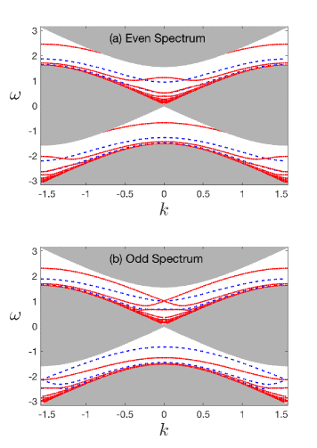
Figure 1: Spectrum of the two-particle walk for $\varphi=1$ and a circle with periodic boundary conditions and lengths $l_{c}=190$ and $l_{c}=191$ for the even and odd spectra, respectively. In the latter, $\varphi_{0}=2\pi$. The grey-shadowed area corresponds to the continuous part of the spectrum, the blue-dashed (red-continuous) lines correspond to fermions (bosons).

In Fig. 1 we show the numerically obtained spectra for $\varphi=1$ in both the even and odd cases, Figs. 1(a) and 1(b) respectively. In solving (14), we have imposed periodic boundary conditions on a line of length $l_{c}=190$ for the even case and $l_{c}=191$ for the odd case, the lengths having been chosen large in order to capture the behaviour in the continuum and also in order to capture not only small size bound states but also large ones. For the even case we have taken $g_{0}=e^{i\varphi_{0}}/2$ with $\varphi_{0}=\pi/2$. The figures reveal the existence of both a continuous spectrum (represented as a grey shadowed area) and a discrete spectrum [the blue-dashed (red-continuous) lines corresponding to fermions (bosons), which we study in the following section]. The continuous part corresponds to plane waves along both coordinates $\rho$ and $\sigma$, and its analytical expression is easy to derive in the limit $l_{c}\rightarrow\infty$ (see Ahlbrecht12 where it is derived and represented).

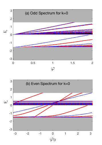
Figure 2: Spectra of the two-particle walk for $\varphi=1$ and $k=0$. In (a) the dependence with $\varphi$ is shown for the odd case, and in (b) the dependence with $\varphi_{0}$ for $\varphi=1$ in the even case is shown. The color code and the rest of details as in Fig. 1.

In Figs. 2 the influence of $\varphi$ for fixed $k=0$ in the odd case, Fig. 2(a), as well as the influence in the even case of $\varphi_{0}$ for fixed $\varphi=1$ and $k=0$, Fig. 2(b), are shown. The increase of $\varphi$ rapidly increases the complexity of the discrete spectrum richness. As for the role of $\varphi_{0}$, it consists in shifting the energy of a part of the eigenstates, not of all of them; we can conclude that the states whose energy is unaffected by $\varphi_{0}$ are those that have null (or nearly null) projection on position $\rho=0$, while it strongly affects states with large projection on $\rho=0$. Another important feature that Fig. 2 reveals is that the bound states energy moves into de continuum as $\varphi$ or $\varphi_{0}$ are changed, which means that in the continuum part of the spectrum there are not only plane waves but also bound states.

IV Bound states

The numerical diagonalization of map (14) provides the complete set of eigenstates. It must be taken into account that, for indistinguishable particles, the wavefunction must verify to be either symmetric or antisymmetric under a change of the particle index, which correspond to bosons and fermions, respectively. In our case, given the definitions $r=u_{1}u_{2}$, $d=u_{1}d_{2}$, $u=d_{1}u_{2}$, $l=d_{1}d_{2}$, the change $1\longleftrightarrow 2$ implies the changes $\left(R_{\rho},D_{\rho},U_{\rho},L_{\rho}\right)\rightarrow\pm\left(R_{-\rho},U_{-\rho},D_{-\rho},L_{-\rho}\right)$ for bosons ($+$) and fermions ($-$).

There is a class of bound states that can be obtained analytically in a very simple manner. These bound sates are those in which the two particles remain at a fixed distance $\rho_{0}$ with a null probability of being at any other distance $\rho\neq\rho_{0}$. Consider first the odd case; take in (14) all the amplitudes null but those for $\rho=\pm 1$, for $k=0$, and the result is $\omega=\varphi$ and

$$U_{+1} = D_{-1}=0,\ \ U_{-1}=D_{+1},$$

$$L_{\pm 1} = R_{\pm 1}-D_{+1},$$ (15)

plus the normalization condition. As there are three degrees of freedom to fix the state, the resulting state is triply degenerated. Three possible states are those for which (i) $L_{+1}=R_{+1}$, $L_{-1}=R_{-1}=0$, and $U_{-1}=D_{+1}=0$ (the molecule only occupies $\rho=+1$), (ii) the same but with $L_{-1}=R_{-1}$ and $L_{+1}=R_{+1}=0$ (the molecule only occupies $\rho=-1$), and (iii) $U_{-1}=D_{+1}\neq 0$ (the molecule occupies both positions $\rho=\pm 1$). Neither of these bound states cannot be classified as boson nor fermion, but from (i) and (ii) above (i.e. $L_{+1}=R_{+1}$ and $L_{-1}=R_{-1}$) one can construct a boson or fermion by choosing $L_{+1}=L_{-1}$ or $L_{+1}=-L_{-1}$, respectively; and state (iii) can be chosen to be a boson by taking $L_{+1}=L_{-1}$. Indeed, as $k$ becomes non null, the degeneracy breaks with two of the states corresponding to fermions and one to a boson, Fig. 1(b).

By assuming that all the amplitudes are null but those for $\rho=\rho_{0}$ with $\left|\rho_{0}\right|\geqslant 3$, for $k=0$ one obtains that the pseudo-energy goes like $\omega=\varphi/\left|\rho_{0}\right|$ and the state amplitudes as

$$U_{\rho_{0}} = D_{\rho_{0}}=0,$$

$$L_{\rho_{0}} = R_{\rho_{0}},$$ (16)

this state being degenerate because $\rho_{0}$ can be either positive or negative. Again, by combining this state with the equivalent one existing at $-\rho_{0}$, a boson and a fermion are constructed. All these bound states are easily identified in the spectrum of Fig. 2(a) because the pseudo-energy goes like $\omega=\varphi/\left|\rho_{0}\right|$.

In the even case, a similar reasoning permits to find several states easily, the simplest being the state of energy $\omega=\varphi_{0}$ when $\rho=0$ and states of energy $\omega=\varphi/\rho_{0}$ when $\left|\rho_{0}\right|\geqslant 2$. Notice that all the bound states we have commented, both in the odd and even cases, are degenerated at $\omega=0$ when $\varphi=0$, see Fig. 2(a), and it is the interaction that breaks this degeneracy. Of course these are not the only bound states, only the simpler.

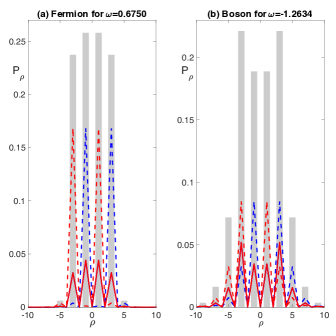
Figure 3: Bound states in the odd case for $\varphi=1$, $k=0$, and $\omega=0.6750$ (left) and $\omega=-1.2634$ (right), which are a fermion and a boson, respectively. The grey bars mark $P_{\rho}$, the total probability as a function of the relative coordinate $\rho$. The dashed-blue and dashed-red lines corresponds to $\left|R\right|^{2}$ and $\left|L\right|^{2}$, respectively, while the full-red line corresponds to $\left|D\right|^{2}=\left|U\right|^{2}$.

Apart from the simple bound states just described, the spectrum reveals the existence of other more complex states extending over several positions along $\rho$, an example of which is given in Fig. 3 where the bound state detailed probability distribution is shown as a function of $\rho$, for both a boson and a fermion, see the figure caption for details. In order to give a feeling of the different bound states, we show in Fig. 4 the total probability distribution as a function of $\rho$ for $\varphi=1$ and $k=0$. The plot shows that most molecules can be calculated by diagonalizing the map on a line with a small total length $l_{c}$, so that our choice $l_{c}=190,191$ is more than correct.

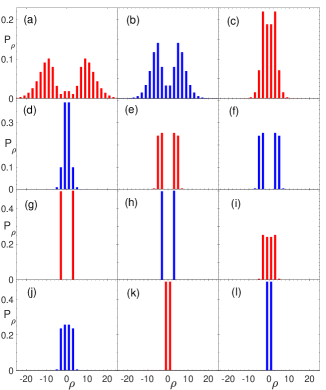
Figure 4: Total probability as a function of $\rho$ for different bound states corresponding to the even case with $\varphi=1$ and $k=0$. The red (blue) graphs correspond to ferminons (bosons), and the states are represented for increasing energies, the frequencies of the states being: (a) -1.499, (b) -1.453, (c) -1.2631, (d) -0.8328, (e) 0.2677, (f) 0.2678, (g) 0.333 (double), (h) 0.333 (double), (i) 0.6546, (j) 0.6750, (k) 1 (triple), (l) 1 (triple). Bound states (c) and (j) were shown in full detail in Fig. 3 above. Notice the different size of the vertical axes in the different rows.

Ahlbrecht et al. Ahlbrecht12 were able to demonstrate that the bound states follow a joint QW on the line. Here we shall not attempt any analytical approach to that but just show numerically that this is the case also in our problem. In order to project into a particular bound state we choose as an initial condition that the two walkers lie in molecules (k) and (l) in Fig. 5, one is a boson and the other is a fermion; further, this initial condition occupies odd positions from $-13$ to $+13$ along the $\sigma$ coordinate (14 occupied sites in total). We choose such extended initial states in order to project most of the probability distribution onto the selected bound states. When the QW is run we clearly see that most of the probability lies on the bound state (see the insets showing that the probability mostly occupies $\rho$ positions corresponding to the bound state, extending very little along this coordinate), and that these bound states behave as expected from the spectrum of Fig. 1(b): notice that at around $k=0$ and $\omega=1$ to the fermion it corresponds a parabolic dispersion relation (that increases the probability distribution width with time, see Fig. 5(b)), while to the boson there correspond two dispersion relations that give a mean velocity to the distribution, see Fig. 5(a), where two wavepackets are seen to travel in opposite directions, each governed by a dispersion relation with a different sign of the velocity. This example shows how to every molecule there corresponds different propagation properties.

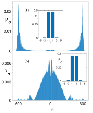
Figure 5: Marginal probability distribution $P_{\sigma}$ versus coordinate $\sigma$ for $\varphi=1$ at $t=500$ corresponding to the odd case; the insets show the marginal probability $P_{\rho}$. The initial coin state is $\left(0,0,1/\sqrt{2},1/\sqrt{2}\right)$, i.e., $\left(0,1\right)$ for the first coin and $\left(1/\sqrt{2},1/\sqrt{2}\right)$ for the second; as for the initial condition, it has been chosen to occupy odd positions from $-13$ to $+13$ along the $\sigma$ coordinate (14 ocupied sites in total) with uniform amplitude. The bound states corresponding to (a) are bosons, while in (b) the bound state is a fermion.

V Attractive vs repulsive interactions

One interesting question is whether there is any clear difference between attractive and repulsive interactions, and certainly there should be if one expects the long-wavelength approximation of the Coulombian QW to capture some of the physics of Coulombian interactions in the continuum. We have seen that as far as the spectrum is involved, the only difference between the two cases consists in changing the pseudo-energy sign. However, by taking a initial condition that does not project on any of the bound-states, which is accomplished by taking a large initial distance between the walkers, one expects to see the difference between attraction and repulsion because of the long range of the interaction. And this is exactly what numerics show: a transient attraction/repulsion between the two walkers that lasts till the diffusion leads to the spatial overlap of the probability distribution of the two walkers, from this time on the subsequent evolution of the probability distribution being no more governed by the Coulombian attraction/repulsion but by the projection onto the different bound states.

In Figs.6 and 7 we show, for attractive and repulsive interactions, the temporal evolution of the mean distance between the particles $\left\langle\rho\right\rangle$ minus the initial distance $\rho_{0}$. They correspond to two distinguishable walkers whose initial positions are centered at $x_{1,2}\left(t=0\right)=\pm 300$, hence $\rho_{0}=600$, the walkers not being sharply localized but extending along the line with a Gaussian distribution of moderate width $\Delta x=10$. The insets in the figures show top views of the probability distributions $P_{x_{1},t}^{x_{2}}$ on the plane $\left(x_{1},x_{2}\right)$ at three selected instants (bright colours correspond to large probability values).

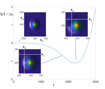
Figure 6: Mean value of the distance between the particles $\left\langle\rho\right\rangle$, referred to the initial distance $\rho_{0}=600$, for two particles initally located at $x_{1,2}\left(t=0\right)=\pm 300$ both having an initial Gaussian distribution of width $\Delta x=10$ (FWHM$=20\ln 2$) and $k_{x}=k_{y}=\pi/4$. The initial coin state is $\left(1,i,-i,1\right)/2$, i.e., $\left(1,-i\right)/\sqrt{2}$ for the first coin and $\left(1,i\right)/\sqrt{2}$ for the second. The insets show a top-view of the probability distribution $P_{x_{1},t}^{x_{2}}$ on the plane $\left(x_{1},x_{2}\right)$ (clear colors correspond to large probability). Notice that the two distributions do not project on each other initially (in the left inset the axes are far apart), the start projecting in the middle inset (the total distribution approaches the origin), and begin to project strongly on the right inset. We took $\varphi=\pi$.

If there were no interaction, diffusion would not make the two particles distribution overlap each other before some time because they are far apart initially, and during these initial stages attraction/repulsion can be captured, as Figs. 6 and 7 show. When diffusion finally makes that the probability distributions mix [this occurs when the total probability distribution reaches the diagonal on the plane $\left(x_{1},x_{2}\right)$, see the insets in Figs. 6 and 7], the subsequent dynamics is governed by that of the bound and unbound states onto which the probability distribution projects, which strongly depends on the initial condition. In order to make these calculations we first looked at the dispersion relation of the non-interacting walk Ahlbrecht12 , and concluded that by taking $k_{x}=k_{y}=\pi/2$ the evolution for $\varphi=0$ is that corresponding to the usual dispersion of a Gaussian wave-packet deValcarcel10 (the wavepacket width increases slowly with time without net motion), which is the ideal situation to isolate the effect of the interaction between particles. But this is not essential, and if one takes different initial values for $k_{x}$ and $k_{y}$, one obtains similar results for the evolution of the distance between the centroids of the probability distributions, even if it may split into several wavepakets. Moreover, the above qualitative conclusion applies equally well when the initial condition is point like, the major difference being that the duration of the Coulombian transient is shorter in this case because of the faster spread of the probability distribution for localized initial states.

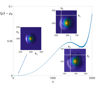
Figure 7: As in Fig. 6 but for $\varphi=-\pi$.

When indistinguishable particles are considered, only the repulsion can be studied as the two particles must have the same charge, and we have tested that the same qualitative conclusions hold.

VI Conclusions

In this article we have introduced the QW of two particles that interact via a long-range Coulombian-like interaction. The novelty with respect to previous work on two-particle QWs lies on the long-range of the interaction as contact interactions are the only ones studied up to know in coined QWs, moreover, in the wider context of continuos-time QWs and Bose-Hubbard two-particle models next-neighbourg or contact interactions are the only ones considered. We have been able to obtain the spectrum of plane waves as well as to derive the bound states, both bosons and fermions, of which we have given some details. We have also shown, numerically, that the bound states follow a joint QW that is governed by the dispersion relation corresponding to those bound states. We have finally discussed on the differences between attractive and repulsive interactions, that better manifest by studying the transient dynamics when the particles lie initially apart enough.

We acknowledge financial support from the Spanish Government and the European Union FEDER through project FIS2014-60715-P.

References

- (1) Richard P. Feynman and A.R. Hibbs, Quantum Mechanics and Path Integrals, International Series in Pure and Applied Physics (McGraw-Hill, 1965).
- (2) Y. Aharonov, L. Davidovich, and N. Zagury, Phys. Rev. A 48, 1687 (1993).
- (3) D. Meyer, J. Stat. Phys. 85, 551 (1996).
- (4) E. Farhi and S. Gutmann, Phys. Rev. A 58, 915 (1998).
- (5) A.M. Childs and J. Goldstone, Phys. Rev. A 70, 042312 (2004).
- (6) V. Kendon, Math. Struct. Comput. Sci. 17, 1169 (2006); Phil. Trans. R. Soc. A 364, 3407 (2006);
- (7) S.E. Venegas-Andraca, Quant. Inf. Proc. 11, 1015 (2012).
- (8) K. Manouchehri and J. Wang, Physical Implementation of Quantum Walks (Springer, 2014).
- (9) Y. Omar, N. Paunkovic, L. Sheridan, and S. Bose, Phys. Rev. A 74, 042304 (2006).
- (10) L. Sheridan, N. Paunković, Y. Omar, and S. Bose, Int. J. Quant. Inf. 4, 573 (2006).
- (11) M. Stefanak, T. Kiss, I. Jex, and B. Mohring, J. Phyes. A: Math. Gen. 39, 14965 (2006).
- (12) P.K. Pathak and G.S. Agrawal, Phys. Rev. A 75, 032351 (2007).
- (13) S. Shiau, R. Joynt, and S. N. Coppersmith, Quant. Inf. and Computation 5, 492 (2005).
- (14) J.K. Gamble, M. Friesen, D. Zhou, R. Joynt, and S. N. Coppersmith, Phys. Rev. A 81, 052313 (2010).
- (15) S.D. Berry and J.B. Wang, Phys. Rev. A 83, 042317 (2011).
- (16) M. Stefanak, S.M. Barnett, B. Kollár, and I. Jex, New Journ. Phys. 13, 033029 (2011).
- (17) A. Ahlbrecht, A. Alberti, D. Meschede, V.B. Scholz, A.H. Werner, and R.F. Werner, New. Journ. Phys. 14, 073050 (2012).
- (18) Y. Lahini, M. Verbin, S.D. Huber, Y. Bromberg, R. Pugatch, and Y. Silberberg, Phys. Rev. A 86, 011603 (2012).
- (19) X. Qin, Y. Ke, X. Guan, Zh. Li, N. Andrei, and Ch. Lee, Phys. Rev. A 90, 062301 (2014).
- (20) A. Beggi, L. Razzoli, and P. Bordone, M.G.A. Paris, Phys. Rev. A 97, 013610 (2018).
- (21) D. Wiater, T. Sowinski, and J. Zakrzewski, Phys. Rev. A 96, 043629 (2017).
- (22) A. Peruzzo, et al. Science 329, 1500 (2010).
- (23) K. Poulios et al., Phys. Rev. Lett. 112, 143604 (2014).
- (24) A.A. Melnikov, and L.E. Fedichkin, Sci. Rep. 6, 34226 (2016).
- (25) I. Siloi et al., Phys. Rev. A 95, 022106 (2017).
- (26) H. Tang et al., arXiv:1704.08242 [quant-ph].
- (27) G.R. Carson, T. Loke, and J.B. Wang, Quant. Inf. Process. 14, 3193 (2015).
- (28) Q. Wang and Z.J. Li, Ann. Phys. 373, 1 (2016).
- (29) A. Bisio, D.M. D’Ariano, N. Mosco, P. Perinotti, and A. Tosini, arXiv:1804.08508 [quant-ph].
- (30) A. Schreiber et al., Science 336, 55 (2012).
- (31) L. Sansoni et al., Phys. Rev. Lett. 108, 010502 (2012).
- (32) J.C. Slater, H. Statz, and G.F. Koster, Phys. Rev. 91, 1323 (1953).
- (33) J. Hubbard, Prc. Roy. Soc. A 276, 238 (1963).
- (34) S.M. Mahajan and A. Thyagaraja, J. Phys. A: Math. Gen. 39, L667 (2006).
- (35) A. Hamo et al. Nature 535, 395 (2016).
- (36) T.D. Mackay, S.D. Bartlett, L.T. Stephenson, and B.C. Sanders, J. Phys. A: Math. Gen. 35, 2745 (2002).
- (37) G.J. de Valcárcel, E. Roldán, and A. Romanelli, New. J. Phys. 12, 123022 (2010).