Radar-based Re-Entry Predictions with very limited tracking capabilities: the GOCE case study

Abstract

The problem of the re-entry predictions of GOCE has been investigated in many different ways and presented in the literature, especially because of the large amount of observational data, mainly radar and GPS, available until the very last part of its decay. The accurate GPS and attitude measurements can be used to compute a POD during the three weeks of decay, which can be exploited to extrapolate the ballistic coefficient evolution of the object, and as a reference trajectory. In previous works the main focus was on the german TIRA radar and on similar tracking sensors, to investigate the capabilities of radar-based orbit determination and ballistic coefficient calibration for re-entry predictions (residual lifetime estimation).

During this work we have carried out additional analysis on radar-based re-entry predictions for GOCE, and for other similar decaying objects on circular and highly inclinated orbits. We focus on the northern european sensor EISCAT UHF radar, located in Tromsø, Norway. This sensor, originally conceived for atmospheric studies of the ionosphere, has been recently considered for space debris applications, for tracking of specific targets, and to support re-entry predictions. The limited tracking capabilities of this sensor poses the problem of establishing to which extent it would be useful to support orbit determination and re-entry predictions, in comparison to what we know about TIRA-like performances.

We have set up a realistic simulation scenario for a re-entry campaign. Re-entry predictions and ballistic coefficient calibrations are performed and compared for TIRA-only, EISCAT-only, and both radar available situations. The results are compared in terms of differences in the orbital states over the total observation time span, in the ballistic coefficient estimation, and in the corresponding re-entry epoch.

The main conclusion is that, provided a minimum amount of necessary observational information, EISCAT-based re-entry predictions are of comparable accuracy to TIRA-based (but also to GPS-based, and TLE-based if TLE errors are properly accounted) corresponding ones. Even if the worse tracking capabilities of the EISCAT sensor are not able to determine an orbit at the same level of accuracy of TIRA, it turned out that the estimated orbits are anyway equivalent in terms of re-entry predictions, if we consider the relevant parameters involved and their effects on the re-entry time. What happens to be very important is the difficulty in predicting both atmospheric and attitude significant variations in between the current epoch of observation and the actual re-entry. For this reason, it is not easy to keep the actual accuracy of the predictions much lower than 10% of the residual lifetime, apart from particular cases with constant area to mass ratio, and low atmospheric environment variations with respect to current models.

A corresponding GOCE ballistic coefficient estimation based on TLE only is presented, and it turns out to be very effective as well. Some critical cases which consist in a minimum amount of observational information, or in difficulties in obtaining OD convergence, are presented, and a list of possible countermeasures is proposed.

An experiment with real EISCAT,TIRA, and TLE data is also presented, for the case of 2012-006K AVUM R/B. Additional experiments with simulated trajectories are presented as well, with analogous results.

1 Introduction

During the ESA GSP “EXPRO+-Benchmarking Re-Entry Prediction Uncertainties” project, we have investigated the problem of the estimation of the GOCE re-entry location, i.e. the re-entry time prediction, on the basis of both continuous GPS measurements and sparse radar tracking information (see Cicalò et al. (2017)). The main result is that, with a reasonable frequency of measurements, radar-based Orbit Determination (OD) is very effective in estimating the average evolution of the spacecraft’s ballistic coefficient, in comparison to the one estimated from continuous GPS measurements, even from a single site. Focus was made on the german TIRA radar of the Fraunhofer institute for High Frequency Physics and Radar Techniques, and on analogous, even though less accurate, sensors. The high orbit accuracy provided by GPS-based Precise Orbit Determination (POD) hides the intrinsic large errors in the dynamical models, atmospheric environment, and attitude behaviour, which are artificially absorbed by the fitted empirical accelerations. These errors re-appear in the radar-based OD under the form of large observational residuals. Even with a very good knowledge of the current position and velocity of the spacecraft, and a good average drag determination, in general it is not possible to predict the future re-entry location with very high accuracy (always much better than 10%). For this reason, guaranteeing observational sessions up to few hours before re-entry is always recommended to reduce the size of re-entry windows. We also attempted to generalize the results obtained for GOCE to similar simulated orbits for objects of different shapes (spherical or cylindrical).

The aim of the present work is to test, via numerical simulations, and also with real data processing, the application of a particular radar-based tracking approach, described in Section 2, for re-entry predictions. This technique consists in the generation of very short tracking passes, typically of few seconds, of a decaying object, to be exploited for OD and ballistic coefficient estimation. In other words, the main purpose of this task is to assess to which extent very short tracks from a high-latitude (polar) radar station can be useful to improve the re-entry predictions of a decaying object, at least for a GOCE-like circular polar orbiter. It is well known that, in many cases, the main source of information during re-entry campaigns are the US Two Line Elements (TLE), for which no related uncertainty information is provided. Thus, it is desirable for an institution such as the European Space Agency to have its independent observational resources. An important goal to be achieved in the near future is to free ESA from the dependency from US TLEs release for re-entry campaigns, as much as possible. A clear step in this direction is not only the increased availability of the german TIRA radar, but also the exploitation of european instruments originally conceived for different purposes such as the EISCAT (European Incoherent Scatter Scientific Association, see Figure 1) facilities, for the observation of decaying objects, and space debris in general (see e.g. Nygrén et al. (2012)). It is straightforward that these European stations are to be preferred with respect to other, less affordable, instruments. The possibility to extensively use the very short tracks of the EISCAT sensors in place of other instruments for re-entry predictions shall be examined in this work, by a comparison of the results obtained from comparable scenarios which include and do not include the short tracks.

This problem can be analyzed from at least three points of view: (i) frequency of re-entry predictions, (ii) drag coefficient estimation, (iii) optimization of resources. These three items are strongly related to each other. A better drag coefficient estimation can be achieved with a higher frequency of observations, which on the one hand corresponds to a higher frequency of possible re-entry predictions, and on the other hand implies a larger exploitation of resources. In general, while during the first part of the decay phase few observational resources should be enough to obtain acceptable re-entry predictions, during the very last part of re-entry (e.g. last 48 hours) it is highly recommended to provide more frequent observational data.

Originally designed for observing the ionosphere by means of the incoherent scatter method, the EISCAT radar sites are more suitable to observe polar orbiters rather than low inclination ones, due to their high latitude location. The main features of the four EISCAT sites are given in the following list:

1. Tromsø(Norway): UHF Transmitter/Receiver at $\sim 928$MHz (a $32$m steerable parabolic dish), and VHF Transmitter/Receiver at $\sim 224$MHz (four $30\times 40$m steerable parabolic cylinder);

2. Kiruna (Sweden): VHF Receiver at $\sim 227$MHz (a $32$m steerable parabolic dish);

3. Sodankylä (Finland): VHF Receiver at $\sim 227$MHz (a $32$m steerable parabolic dish);

4. Longyearbyen (Norway): UHF Transmitter/Receiver at $\sim 500$MHz (a $32$m steerable parabolic dish, and a $42$m fixed parabolic dish).

In the following, we will focus on the EISCAT UHF radar working at $930$MHz frequency located in Tromsø, Norway.

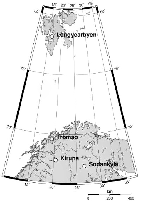
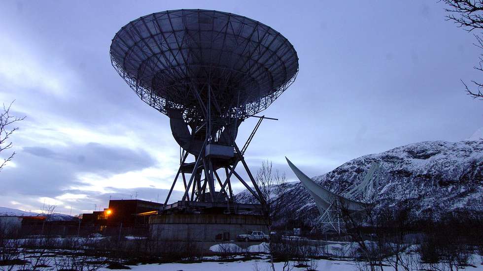
Figure 1: Left: EISCAT facilities map. Right: EISCAT UHF radar at Tromsø

2 EISCAT UHF sensor and main features

Three important references concerning the employment of the EISCAT sensors for space objects observations are Nygrén et al. (2012), Markkanen et al. (2013) and Vierinen & Krag (2017). In particular, the sensor which has to be dedicated mainly to tracking observations is the EISCAT UHF radar working at $930$MHz frequency located in Tromsø, Norway. Due to slow antenna motors not capable to smoothly track a target, the radar measurement strategy is based on a scheduled “point-and-steer” technique, and the peculiarity of this tracking system resides in the very short length of the measured observation sets, of few seconds. This is quite different from standard radar systems techniques (e.g. TIRA) that typically produce continuous observational tracks of several minutes Lemmens et al. (2014).

In order to be able to test the capabilities of such a particular measurement system for re-entry predictions, we shall need to identify the general characteristics of the instrument and of the technique, and to appropriately traduce them under the form of computed observables to be implemented in our Simulation and Orbit Determination software.

According to Vierinen & Krag (2017), we can identify and define the following main features:

1. Location of the sensor $69.58649229^{\circ}N$, $19.22592538^{\circ}E$, $85.554$m

2. Measurement types and expected accuracies Range - approximately $15$m $1\sigma$ errors (as two-way measurement); Range-rate (Doppler shift) - approximately $1$m/s $1\sigma$ errors (as instantaneous measurements); Azimuth/Elevation - no accurate measurement is possible (no mono-pulse feed available).

3. Visibility conditions and measurement frequency Elevation threshold $30^{\circ}$; Dish steering speed $\sim 1.3^{\circ}$/s, the antenna controller cannot smoothly track targets, it can only move to a position and stop there.

The system can be used for limited tracking observations of targets with approximately known orbital elements. The tracking is done using a technique which involves poiting to a location where the target will approximately be and wait for it to pass. Once a preliminary orbital information is available, for example from TLE or other sources, it is possible to estimate the maximum number of points that the antenna can keep up with, i.e. that it is able to steer, point and wait until the object passes through the beam, within the total time span during which the object is potentially visible over the sensor (elevation greater than $30^{\circ}$). In (Vierinen & Krag, 2017, Fig.2.6 and Fig.2.7) there are two examples, showing that the antenna is capable to keep up with one steer-and-point every $\sim 1$ minute, and that the object is expected to pass through the beam for very few seconds. As a result, we have a single measurement “spot” per fixed pointing position consisting of few seconds range and range-rate data. Figure 2 is a graphical representation of this technique, in comparison with standard countinous smooth tracking of few minutes duration.

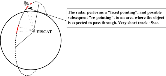
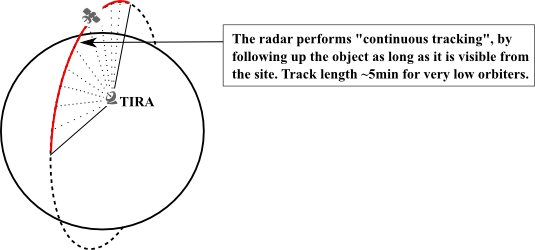
Figure 2: Left: EISCAT limited tracking capabilities. Right: TIRA standard tracking capabilities.

For objects with an orbit high enough to stay over the station for several minutes (e.g. $5$min) it is possible to perform multiple observation spots and to form a tracklet for orbit determination purposes, which can be comparable to a continous tracking pass. However, this is not possible for very low orbiters, such as GOCE or any low circular polar orbiter during decay phase. We will see in the following that for these objects the visibility contraints are such that it is possible to get only one spot per pass.

In this work, we need to focus on re-entry predictions, and in particular on low circular polar orbiters and their ballistic coefficient calibration. A basic comparison with standard radar systems’ features at this point is mandatory. According to Lemmens et al. (2014), Bastida Virgili et al. (2014), and as reported in Cicalò et al. (2017), conventional radar systems can be effectively used for re-entry predictions calibrations. Depending on the geographical location of the radar site, and on the orbital features of the tracked object, different visibility conditions occur. What we can assume for acceptable visibility conditions is a minimum elevation of the detected object over the local horizon of at least $2-3^{\circ}$, on condition that enough information for the calibration of atmospheric refraction is available. For instance, the typical length of a tracking pass is of few minutes for very low orbiters, while the frequency of visibility of subsequent passes from the same station strongly depends on its latitude. Tracking passes which reach a higher elevation peak are preferable, e.g. greater than $10^{\circ}$, since they usually contain more information on the orbit, the atmospheric refraction error is lower, and also provide a lower minimum range distance. As regards the nominal accuracies that can be achieved by standard tracking instruments, values for measurements error’s RMS (noise) around $10-30$m for range and $0.01-0.03^{\circ}$ for azimuth/elevation are commonly considered acceptable to perform good re-entry predictions calibration. In fact, even better values for both measurement’s noise and bias are in principle achievable with high quality radar like TIRA, but extended body uncertainties must be taken into account for large objects, and the presence of large dynamical model’s errors at very low altitudes ends up to dominate the measurement’s errors over long time spans.

In conclusion, the main difference between EISCAT UHF sensor and the standard radar considered so far, resides in the high elevation threshold, in the lack of continuous tracking capabilities and in the low accuracy direction angle information. We will analyse in the following sections how these features can affect the orbit determination and ballistic coefficient calibration problems, and to which extent we can effectively obtain useful information for re-entry predictions.

3 Examples from 2012-006K AVUM R/B real data

As reported in Vierinen & Krag (2017), several experimental tracking observations have been performed with EISCAT, on selected targets, to test EISCAT UHF capabilities for orbital elements determination. As mentioned before, the tracking program utilizes already available TLE orbital elements to plan an antenna scan for tracking of objects. In particular, the selected target 2012-006K VEGA AVUM R/B is of special interest for our study, because it was a re-entry object.

According to the ESA DISCOS database, the 2012-006K AVUM rocket body had a nominal mass of $960$kg, with an approximate shape of $1.9\times 1.7\times 1.9$m³, and an average cross sectional area of $2.162$m² (Figure 3).

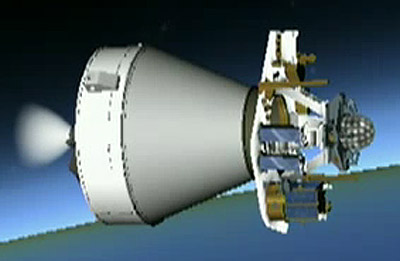
Figure 3: 2012-006K AVUM R/B.

The object re-entered on 2016-11-02. We show on Table 1 the TLE osculating orbital elements on 2016-10-13, 20 days before re-entry, when the minimum altitude of the object was around $210$km.

Table 1: TLE 2012-006K osculating keplerian elements on 2016-10-13 at 19:48:43 UTC, in GCRS

a	e	i	$\Omega$	$\omega$	M
$6649.594\,$km	$8.1817\times 10^{-3}$	$69.3784^{\circ}$	$246.4754^{\circ}$	$176.8664^{\circ}$	$183.2227^{\circ}$

Within this work, ESA provided us with one TIRA pass and four EISCAT passes for 2012-006K close to re-entry. Main information on passes are gathered in Table 2.

Table 2: Summary of TIRA (T1) and EISCAT UHF (E1-E4) tracking passes provided by ESA as CFI

Pass	Obs. type	Data start UTC	Data end UTC
T1	$\rho$,$\dot{\rho}$,$Az$,$El$	2016-10-20 14:50:06	2016-10-20 14:56:09
E1	$\rho$,$\dot{\rho}$	2016-10-21 16:19:48.98	2016-10-21 16:19:50.38
E2	$\rho$,$\dot{\rho}$	2016-10-22 16:09:53.32	2016-10-22 16:09:55.50
E3	$\rho$,$\dot{\rho}$	2016-10-22 19:12:27.81	2016-10-22 19:12:29.88
E4	$\rho$,$\dot{\rho}$	2016-11-01 15:59:48.26	2016-11-01 15:59:50.00

By combining the TIRA and EISCAT passes in different ways we can perform OD and ballistic coefficient calibration, in order to obtain different re-entry predictions. The main dynamical assumptions for the data processing consists in

• a static gravity field up to degree and order 16,

• luni-solar gravitational perturbations,

• a non gravitational drag acceleration:

  $$\mathbf{a}_{drag}=-\frac{1}{2}B\rho v_{r}^{2}\hat{\mathbf{v}}_{r}$$ (1)

  where $\rho$ is the atmospheric density at the object’s location, modeled with NRLMSISE00, using daily and 81d averaged F10.7 solar flux indices, and daily and 3h Ap geomagnetic indices as space weather proxies. $B=C_{d}A/m$ is the ballistic coefficient, assumed to be constant over a single propagation (3DOF approach), $A$ is the reference area of the spacecraft, $C_{d}$ is the drag coefficient, $m$ is the satellite mass, $\hat{\mathbf{v}}_{r}$ is the direction of the relative velocity of the spacecraft with respect to the atmosphere and $v_{r}=|\mathbf{v}_{r}|$. For the relative velocity computation, we assume that the atmosphere is rotating fixed with the Earth Montenbruck & Gill (2005).

In this case, the preliminary information for the orbital state solution (first guess) is always based on the available TLEs, tipically chosen at an apoch close to the middle of the observational interval, while a preliminary value for the drag coefficient $C_{d}$ is around 4.1, for a total of 6+1 parameters to be determined in each OD solution (6 initial conditions and 1 ballistic coefficient).

We have combined three re-entry prediction scenarios, summarized in Table 3.

Table 3: Re-entry prediction scenarios for 2012-006K with the available radar tracks.

scen	passes	total obs. $\Delta T$	residual lifetime from last obs
			to nominal re-entry (nov-2)
1	T1 + E1	$\sim 25$h	$\sim 12$h
2	E1 + E2 + E3	$\sim 27$h	$\sim 11$h
3	T1 + E1 + E2 + E3	$\sim 52$h	$\sim 11$h

The main results for the three re-entry prediction scenario are described in Table 4.

Table 4: Summary of main results for TIRA + EISCAT UHF re-entry predictions of 2012-006K. AP stands for the application of an A-Priori constraint on the initial conditions of 1km in position and 1m/s in velocity (TLE-based). NM stands for Not Mandatory, i.e. the OD scenario is stable.

scen	AP	residuals RMS	estim. $C_{d}A$	re-entry epoch
				UTC (at 90km)
1	Y	T1($\rho$,$Az$,$El$): $10.4$m, $0.0059^{\circ}$, $0.0067^{\circ}$	$8.8373\,$m2	11-03 $\sim$19:56
	(NM)	E1($\rho$,$\dot{\rho}$): $11.7$m, $1.8$m/s
2	Y	E1($\rho$,$\dot{\rho}$): $11.1$m, $1.8$m/s	$8.7332\,$m2	11-03 $\sim$22:00
		E2($\rho$,$\dot{\rho}$): $11.5$m, $1.1$m/s
		E3($\rho$,$\dot{\rho}$): $9.6$m, $1.0$m/s
3	Y	T1($\rho$,$Az$,$El$): $13.5$m, $0.015^{\circ}$, $0.014^{\circ}$	$9.0684\,$m2	11-03 $\sim$11:51
	(NM)	E1($\rho$,$\dot{\rho}$): $66.8$m, $4.5$m/s
		E2($\rho$,$\dot{\rho}$): $28.8$m, $11.5$m/s
		E3($\rho$,$\dot{\rho}$): $17.7$m, $6.3$m/s

As we can see from Table 4, the scenario 2, that does not include the TIRA pass, needs an a priori assumption on the initial conditions error to be included in the fit to obtain stable convergence. In this case the assumption consists in a 1km 3D position and 1m/s 3D velocity a priori covariance matrix, which may be reasonable for the TLE first guess state. This can be understood if we consider that one TIRA pass consists of $\sim 5$ minutes of accurate range, azimuth and elevation measurements, thus containing a quite significant amount of orbital information, while one EISCAT pass basically consists of only one “spot” of range and range-rate data. Since the full OD solution has 7 solve-for parameters, this means that only three EISCAT tracks are not enough to have a full solution with stable differential corrections, and even though in both scenarios 2 and 3 we used the same TLE as first guess for the initial conditions, the case 2 contains too few data and additional information on the orbit is needed. This will be discussed in more details in the following Section 4.3.

As regards the fourth EISCAT track on 2016-11-01, on the one hand it is very close to re-entry and on the other hand it is very far from the previous observations available ($\sim 10$ days). We believe that a calibration with only these data and over a such long time span would be a quite unrealistic and unlucky situation. For a re-entry prediction to be computed during the very last day of decay, a calibration time span at the order of less than one day should be more suitable. In order to try to fit this radar track as it would have been done in reality, we can define a re-entry prediction scenario mixing TLEs and the EISCAT track (Table 5). A standard weight of 1km and 1m/s is applied to the fitted TLEs (see also Section 5).

Table 5: Re-entry prediction scenarios for 2012-006K with the last available radar track and two TLEs.

scen	passes	total obs. $\Delta T$	residual lifetime from last obs
			to nominal re-entry (nov-2)
4	TLE1(10-31$\sim$20:32) +	$\sim 19$h	$\sim 12$h
	TLE2(11-1$\sim$03:53) + E4

The main results for the three re-entry prediction scenario are described in Table 6.

Table 6: Summary of main results for TLE + EISCAT UHF re-entry predictions of 2012-006K

scen	residuals RMS	estim. $C_{d}A$	re-entry epoch
			UTC (at 90km)
4	TLEs(pos,vel): $170$m, $0.2$m/s	$9.5235\,$m2	11-02$\sim$04:57
	E4($\rho$,$\dot{\rho}$): $12.9$m, $1.8$m/s

4 Re-Entry predictions simulations with GOCE POD

In order to perform a deeper analysis on the performances and capabilities of the particular radar measurement system previously introduced, we can set up a reliable simulation scenario, as we have done in Cicalò et al. (2017) for the GOCE spacecraft and other simulated objects. The test case scenario that we want to consider shall consist of a dynamical scenario, i.e. the orbiting object’s main features, and an observational scenario, i.e. the set of data available. We are going to focus on the typical case of a high inclination (polar) LEO in an almost circular orbit at very low altitude, which is decaying to re-entry in few weeks or days.

The first thing to be defined is the list of dynamical assumptions for the orbit of the object that we are going to consider and the forces acting on it, e.g. consisting in a static gravity field up to a suitable degree and order, planetary perturbations, drag perturbations with a ballistic coefficient to be estimated during the orbit determination process. The second step in the definition of the tests is the definition of the observational scenarios. In order to be able to perform a sensitivity analysis with respect to different situations, which means to different availability of observational data, we will need to consider several possibilities in terms of active/inactive radar sites, released TLEs, and additional very short tracks (VST). Thus, a scenario would consist of a set of radar tracking passes, TLEs and whatever additional useful measurement on the orbiting object. To each particular scenario corresponds an orbit determination and a ballistic coefficient estimation, necessary to calibrate a future re-entry prediction. A “re-entry campaign” can thus be simulated by considering a set of subsequent observational scenarios with observations available up to the very last orbits before the object’s re-entry in the lower atmosphere. As extensively done in Cicalò et al. (2017) for the case of single- vs. multi-sensor scenarios, here we want to perform the same kind of tests to compare the cases of observational scenarios including and not including EISCAT’s very short tracks for re-entry predictions. In practice, two different scenarios are considered comparable if they have the same epoch of prediction, i.e. if their last observational data available is more or less at the same epoch. Given two comparable scenarios, we are able to perform a standard OD and ballistic coefficient estimation with the data available for each of them. Two resulting re-entry predictions can be computed, which may be significantly different mainly depending on the total time span of the chosen observations and on the atmospheric model adopted. To the purpose of a reliable and correct comparison between different scenarios, we can make use of the following quantities: the nominal predicted re-entry epoch (conventionally at 90km altitude), the absolute and relative re-entry time error (by exploiting a priori information) with respect to the total re-entry residual lifetime, and the post-fit measurements residuals. Moreover, if enough information is available on the orbit of the re-entering object, then such an orbit can be used as a reference for comparison with the fitted OD solution, and as a source to extrapolate a refined ballistic coefficient’s behavior, e.g. with a suitable piece-wise constant (PWC) function. For example reference orbits can be the accurate GPS-based POD in the GOCE case Gini et al. (2014), the simulated orbit if the trajectory is generated within the whole test process, or just the released TLE states (see Section 5). The behavior of the ballistic coefficient obtained from such richer amount of information on the decaying object, can then be compared with the one obtained from the radar observational scenarios defined before, which contain only sparse data from different sources.

We have already shown in Cicalò et al. (2017) that, provided a reasonable frequency of observations, radar-based re-entry predictions calibrations are very effective in capturing the average drag effect over the time span covered by the measurements. The most important lesson learned from that study was the evidence of the dominance of dynamical model’s errors at decaying altitudes (typically 100-300km), due for instance to the difficulties in having very accurate atmospheric density models available and in accurately predicting significant attitude variation. Errors at the order of 10-20% are commonly found, a particular density model can be better than another for a particular range of altitudes, or for a particular period of time, depending on solar flux and geomagnetic storms events, but none of them can be considered always better than the others Pardini et al. (2004). The differences between two given density models over a fixed time span are not only given by a simple constant bias. For this reason, even if the ballistic coefficient estimation does take into account the correction of a constant bias over a fixed time span, and this correction is quite effective in absorbing part of the mis-modeled dynamics, this bias is not enough to compensate for all the errors in the atmospheric density, both on shorter time intervals and over the time span from the epoch of prediction to the actual re-entry. Thus, the adoption of different density models could in principle lead to significantly different re-entry predictions. Finally, particular changes in the attitude motion of elongated, or just asimmetric, objects could lead to large variations of the average ballistic coefficient and thus of the re-entry time.

4.1 Main assumptions

Also in this case, the main dynamical assumptions for the data processing consists in: a static gravity field up to degree and order 16, luni-solar gravitational perturbations, a 3DOF non gravitational drag acceleration with atmospheric density model NRLMSISE00, using daily and 81d averaged F10.7 solar flux indices, and daily and 3h Ap geomagnetic indices as space weather proxies. Reference Cicalò et al. (2017) holds for the assumptions in the simulation of the TIRA radar measurements: elevation threshold of $2^{\circ}$, random generated noise of 10m in range and $0.01^{\circ}$ in azimuth and elevation, using the GOCE POD as reference trajectory. The simulated TIRA passes which have a maximum elevation peak lower than $10^{\circ}$ are generally not used here. No addition of tropospheric refraction effects is considered in the simulations, assuming that they are already removed to a level lower than the considered noise (see e.g. Montenbruck & Gill (2005)). A deeper dedicated analysis on this latter topic is considered beyond the purposes of this work.

As regards the specific EISCAT UHF measurements simulation, we need to take the cue from what is described in Vierinen & Krag (2017), and summarized in Section 2. Given an elevation threshold of $30^{\circ}$, we assume to be able to schedule an antenna scan per minute of visibility over the station. In the case of a low orbiter such as GOCE, the duration of a visibility from EISCAT over $30^{\circ}$ of elevation is of the order of one minute (see results below). This implies that in general we can assume to be able to point the radar around the middle of the expected pass, and wait for the object to pass through the beam. The duration of a satellite passing through the radar beam is a few second, we assume to take 2 seconds of range and range-rate measurements, with a frequency of 0.1s. Note that a shorter frequency of 0.01s could also be used, but such track is so short that we expect it to be more or less equivalent to a single measurement of range and range-rate. The simulated noise for such measurements is of 15m in range and 1m/s in range-rate. Finally, no observation of azimuth and elevation is used, even if we believe that at least a low accuracy information just from antenna pointing could be useful in some cases (see Section 4.3).

A visual representation of the visibility of GOCE from TIRA and EISCAT UHF is given in Figure 4, for the three weeks of decay (from MJD 56586 to MJD 56606). The maximum elevation peaks are also shown. The average duration of the TIRA passes is $\sim 5.8$min, while the average duration of the visibility over the EISCAT UHF radar is $\sim 1.3$min. As already stated, we assume to be able to get just one spot of $\sim 2$ seconds per pass, around the middle of each pass. Another drawback of the high elevation threshold of $30^{\circ}$ is the possibility to have larger gaps of 24 hours between two subsequent observations. It is interesting to note that the EISCAT and TIRA tracks are very close together. The EISCAT sensor has a higher latitude of $\sim 20^{\circ}$ with respect to TIRA, and a different longitude of $\sim 12^{\circ}$. In principle, due to the higher latitude, without the constraints on the elevation threshold and on the minimum elevation peak, the EISCAT sensor would allow for much more visibility and a much higher frequency of passes. However, in every case the geometrical conditions turned out to be such that the EISCAT and TIRA passes with the highest elevation peaks are always not more distant than one orbit, and these are also the only ones that satisfy the former elevation constraints (shown in Figure 4).

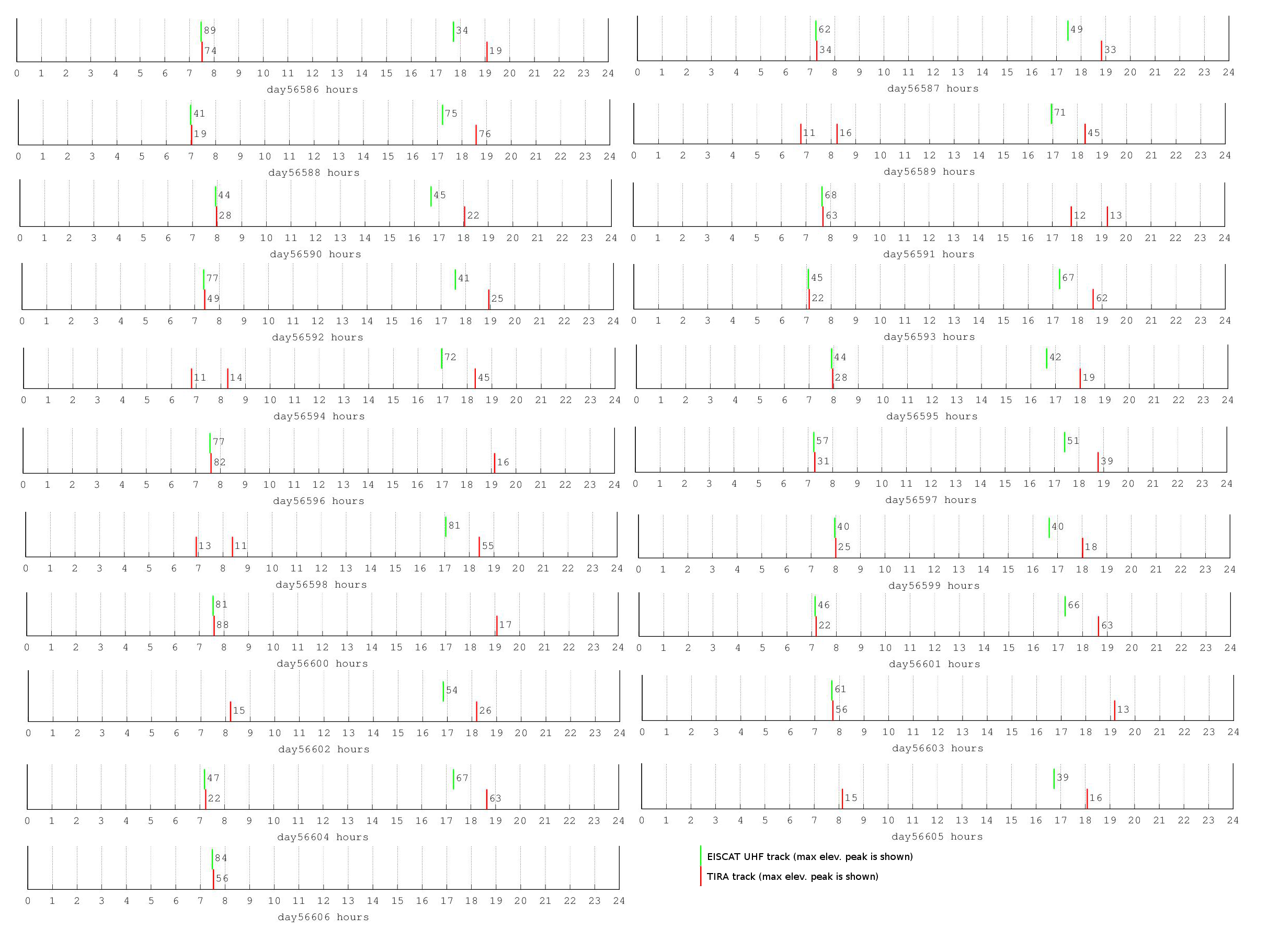
Figure 4: Visual representation of tracking passes from TIRA (red) and EISCAT UHF (green) during the three weeks of GOCE decay (time is in MJD). Maximum elevation peaks of passes are shown in deg, discarding passes with elevation peaks of less than 10^∘.

The basic idea is the same as the one described in Cicalò et al. (2017) for the case of TIRA-only and many sensors re-entry prediction scenarios. The reference trajectory (GOCE POD) is fully exploited to estimate a refined piecewise constant ballistic coefficient that is able to compensate the mis-modeled non gravitational perturbations up to a certain level of accuracy. A suitable subinterval of 30min was considered a good value to reconstruct the variations the ballistic coefficient from the orbit, but also shorter subintervals were possible. We showed that with a station like TIRA, OD and ballistic coefficient calibration with radar passes over 24-48h are very effective in estimating the average behavior of the ballistic coefficient and a good re-entry trajectory, in comparison with the 30min PWC coefficient and with the POD orbit itself. As we approach the last part of re-entry, calibrations over shorter time intervals (e.g. 12h) are also effective.

As an example, we show in Table 7 the results for the OD scenario which includes the first four TIRA passes during re-entry days 1 and 2, in terms of comparison with the reference orbit. In Figure 5 we can see the estimated ballistic coefficient in comparison with the POD-based 30min PWC coefficient. The corresponding estimated re-entry epoch is Nov-11 at $\sim$11:24 UTC.

Table 7: RMS differences between TIRA-based estimated orbit and POD over re-entry days 1 and 2, in the R-T-W system and in osculating keplerian elements semimajor axis $a$, eccentricity $e$, and mean argument of latitude $\omega+M$

	$\Delta\mathbf{x}_{R}$	$\Delta\mathbf{x}_{T}$	$\Delta\mathbf{x}_{W}$	$\Delta\mathbf{v}_{R}$	$\Delta\mathbf{v}_{T}$	$\Delta\mathbf{v}_{W}$
RMS	192.0m	542.7m	81.7m	0.5m/s	0.2m/s	0.1m/s
	$\Delta a$	$\Delta e$	$\Delta(\omega+M)$
RMS	10.3m	$3.4\times 10^{-5}$	$0.0032^{\circ}$

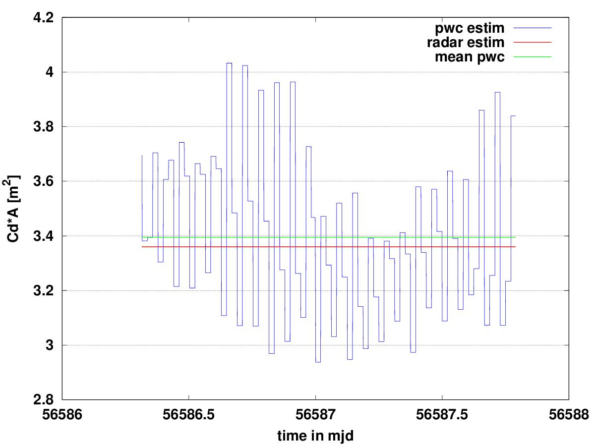
Figure 5: TIRA-based ballistic coefficient estimation (in red) over re-entry days 1 and 2, compared with POD-based 30min PWC coefficient (in blue). Relative difference with respect the mean value (in green) is $\sim 1\%$.

We show in Figure 6 the case of a TIRA-only simulated re-entry campaign, with ballistic coefficient estimations over intervals of $\sim$36 hours, compared with the 30min PWC coefficient from POD. More specific results, in terms of differences with respect to POD are shown in Figures 7, 8, 9. Note that for the evaluation of the error in the re-entry time we have used the residual lifetime relative error formula: $(t_{re}-t_{re}^{tr})/(t_{re}^{tr}-t_{pred})\cdot 100$, where $t_{re}$ and $t_{re}^{tr}$ are the estimated and true re-entry epochs, respectively, and $t_{pred}$ is the epoch of prediction (i.e. the epoch of the last data available).

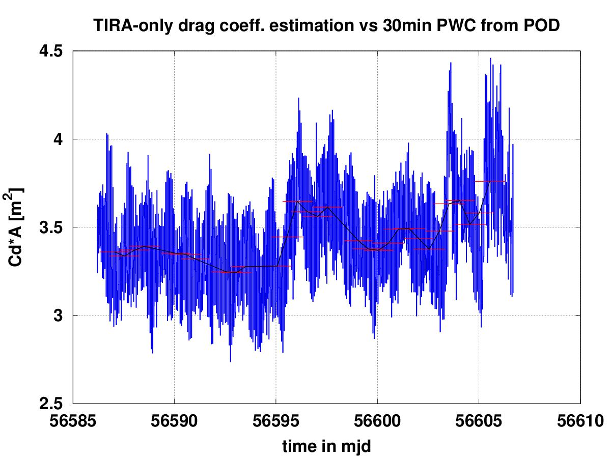
Figure 6: TIRA-only ballistic coefficient estimation over intervals of  36 hours (in red), compared with 30min PWC coefficient from POD (in blue).

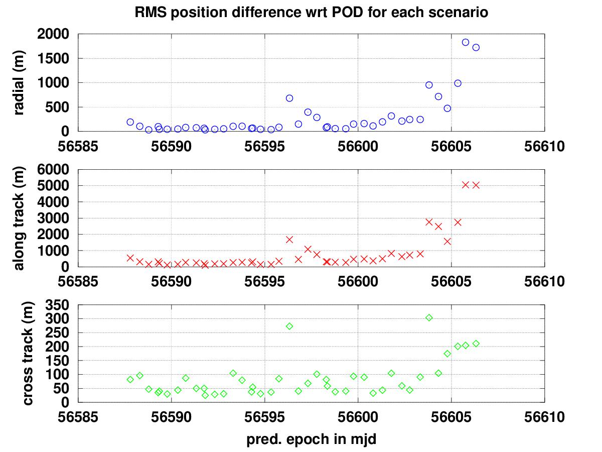
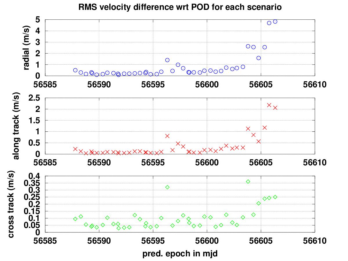
Figure 7: RMS of position (left) and velocity (right) differences w.r.t. POD for each TIRA-based prediction scenario.

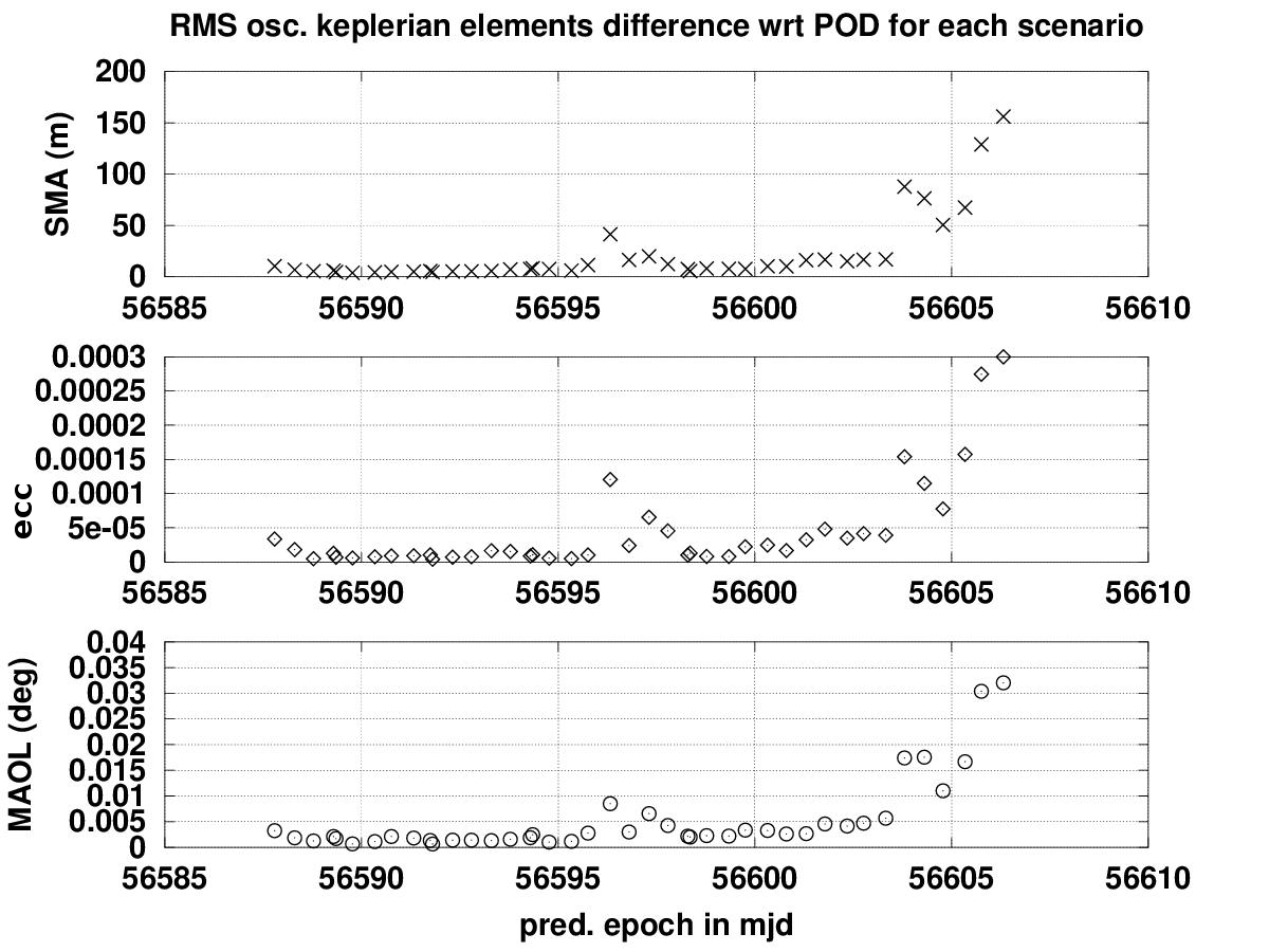
Figure 8: RMS of osculating Keplerian elements differences w.r.t. POD for each TIRA-based prediction scenario.

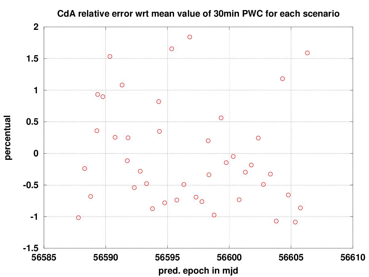
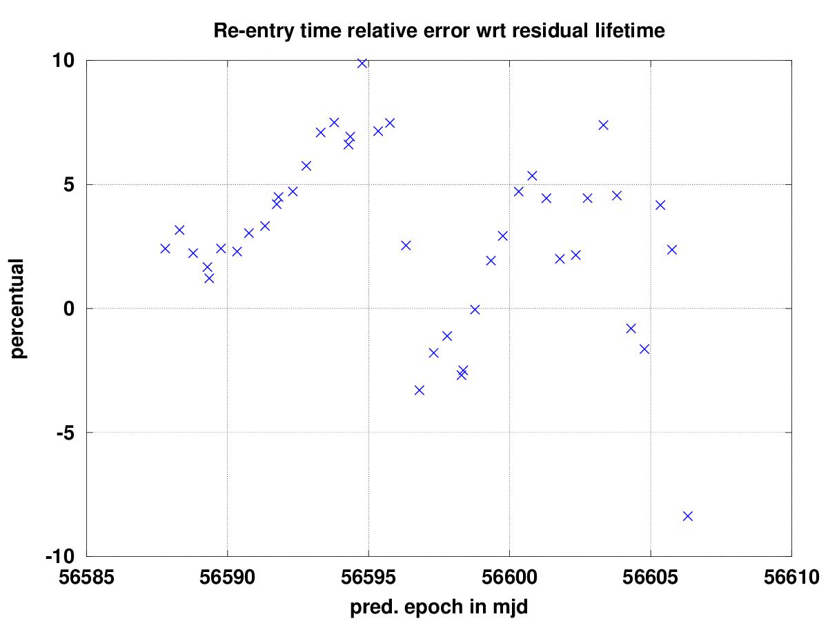
Figure 9: lEFT: $C_{d}A$ coefficient percentual relative difference with respect to the mean of the 30min PWC coefficient over each TIRA-based prediction scenario’s observation time span. Right: Residual lifetime percentual relative errors for each prediction of the simulated TIRA-based re-entry campaign.

In the case of EISCAT UHF radar alone, we have already mentioned the fact that, since we do not have accurate azimuth/elevation measurements, and since the duration of tracking is very short, the data contained in only two or three subsequent passes contain too little information to obtain a full 7-dim OD solution. We will discuss these cases in Section 4.3. In this section we focus only on EISCAT-based solutions with four consecutive tracks, which cover about 36h, and in some cases about 48h.

For comparison with Table 7 and Figure 5, we show in Table 8 the results for the OD scenario which includes the first four EISCAT tracks during re-entry days 1 and 2, in terms of comparison with the reference orbit, while the estimated ballistic coefficient in comparison with the POD-based 30min PWC coefficient has a relative difference of $\sim 1.3\%$. The corresponding estimated re-entry epoch is Nov-11 at $\sim$12:46 UTC. As we can notice, the TIRA-based vs. EISCAT-based corresponding results are very much aligned in terms of re-entry prediction, even though the orbital differences in the RTW system are significantly different. In other words, over a comparable total observation time span, the TIRA-based and EISCAT-based re-entry predictions are equivalent. We will see that this is true for the entire simulated campaign. We will come back to this point later in Section 4.2.

Table 8: RMS differences between EISCAT-based estimated orbit and POD over re-entry days 1 and 2, in the R-T-W system and in osculating keplerian elements semimajor axis $a$, eccentricity $e$, and mean argument of latitude $\omega+M$

	$\Delta\mathbf{x}_{R}$	$\Delta\mathbf{x}_{T}$	$\Delta\mathbf{x}_{W}$	$\Delta\mathbf{v}_{R}$	$\Delta\mathbf{v}_{T}$	$\Delta\mathbf{v}_{W}$
RMS	797.1m	2620.9m	808.6m	2.6m/s	0.9m/s	0.9m/s
	$\Delta a$	$\Delta e$	$\Delta(\omega+M)$
RMS	12.2m	$1.2\times 10^{-4}$	$0.016^{\circ}$

We show in Figure 10 an EISCAT-only simulated re-entry campaign, with ballistic coefficient estimations over intervals of $\sim 36$hours, compared with the 30min PWC coefficient from POD. More specific results, in terms of differences with respect to POD are shown in Figures 11, 12, 13. As we can see from a comparison with the corresponding TIRA-only results, there is a very good agreement in the ballistic coefficient calibration and in the re-entry epoch estimation. Other interesting results is that while in the first part of decay phase (e.g. first week), where the dynamical mis-modelings are lower, the TIRA-based orbital solutions are significantly better than the EISCAT-based ones, meaning that the observational features still dominates over the dynamical errors. On the contrary, during the last part of decay (last week), both TIRA and EISCAT based orbital solutions tend to be of comparable accuracy, meaning that the dynamical errors dominate over the observational features. Interestingly, we have seen that in all cases the TIRA-based and EISCAT-based predictions are analogous. This will be explained in Section 4.2.

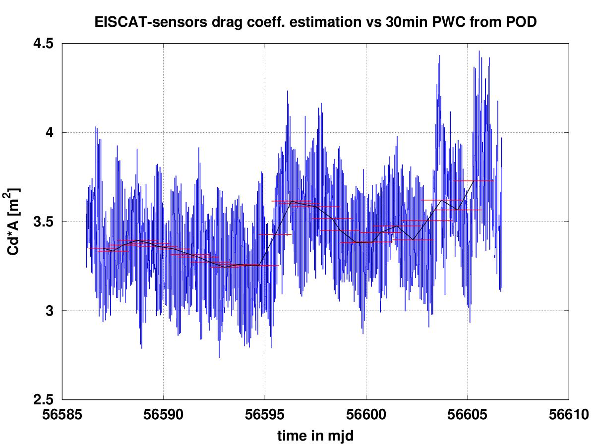
Figure 10: EISCAT-only ballistic coefficient estimation over intervals of  36 hours (in red), compared with 30min PWC coefficient from POD (in blue).

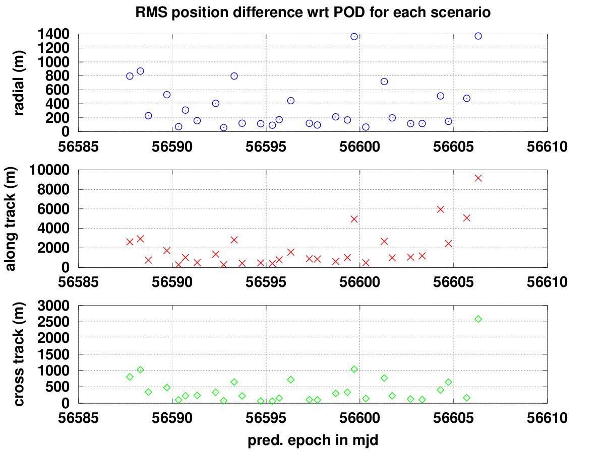
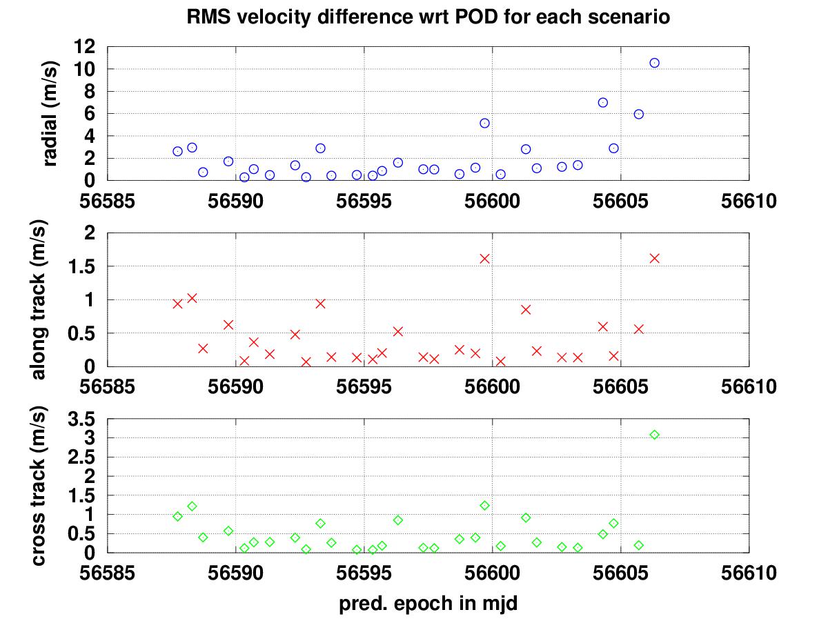
Figure 11: RMS of position (left) and velocity (right) differences w.r.t. POD for each EISCAT-based prediction scenario.

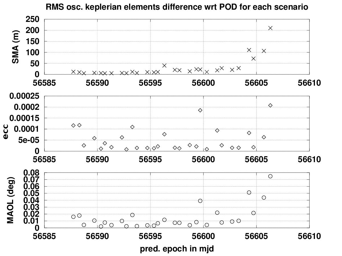
Figure 12: RMS of osculating Keplerian elements differences w.r.t. POD for each EISCAT-based prediction scenario.

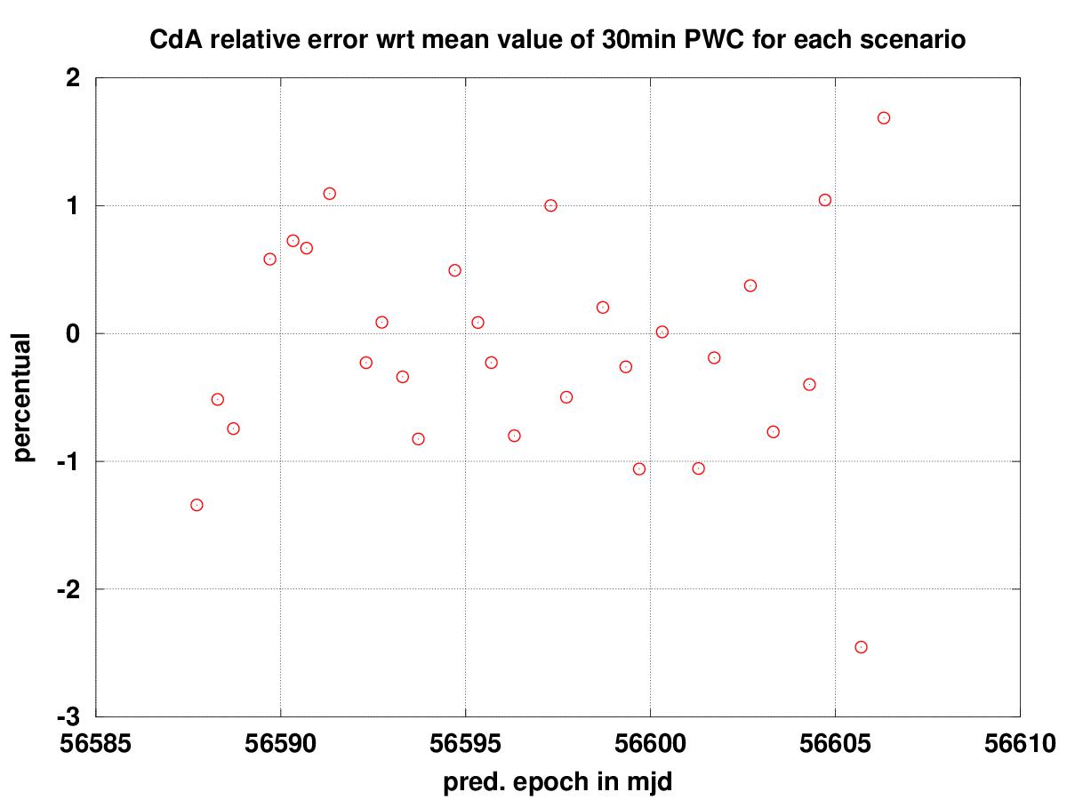
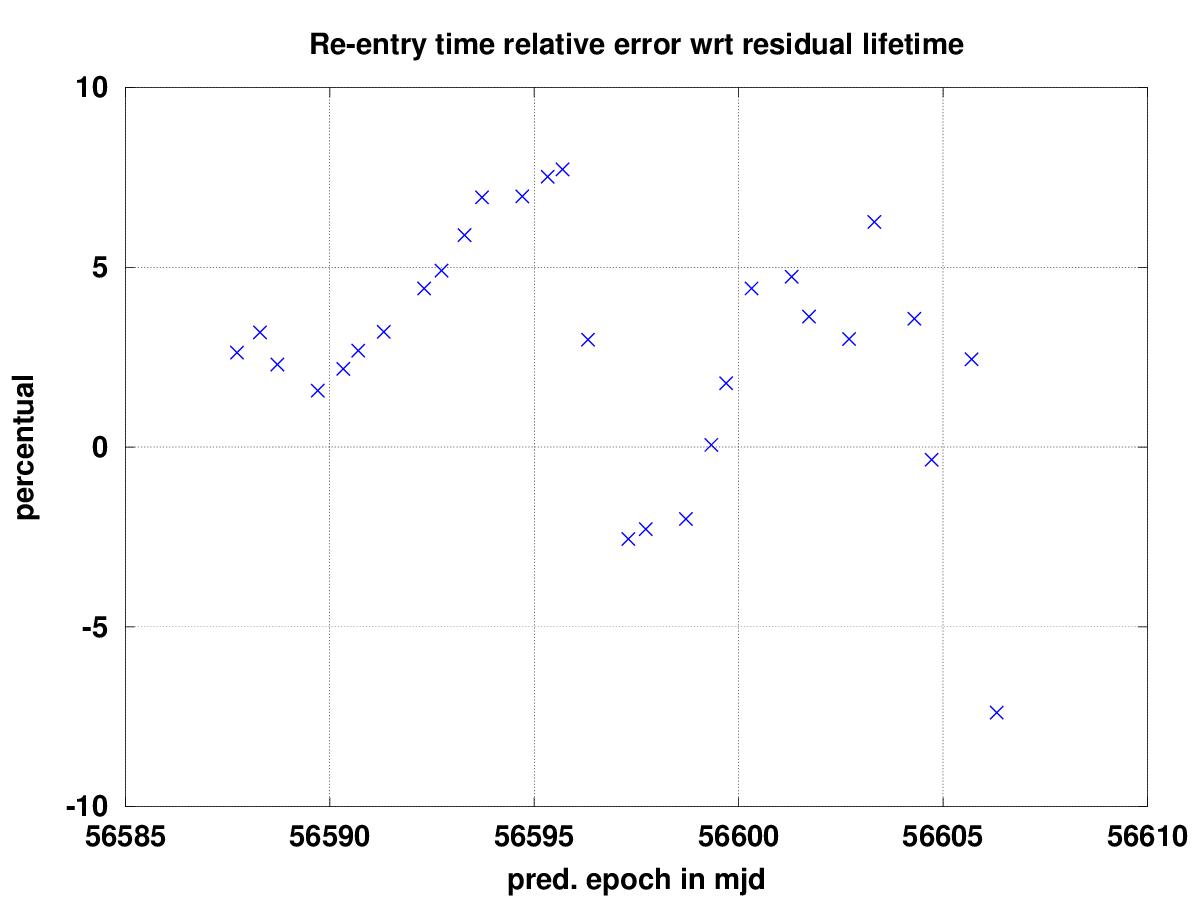
Figure 13: Left: $C_{d}A$ coefficient percentual relative difference with respect to the mean of the 30min PWC coefficient over each EISCAT-based prediction scenario’s observation time span. Right: Residual lifetime percentual relative errors for each prediction of the simulated EISCAT-based re-entry campaign.

We can now discuss these results in terms of (i) frequency of re-entry predictions, (ii) drag coefficient estimation, and (iii) optimization of resources.

1. Frequency of re-entry predictions: we have already discussed that the TIRA and EISCAT passes are generally close in time (Figure 4), due to the quite close longitudes of the two stations and the geometrical constraints. Moreover, due to the high elevation threshold, the EISCAT sensor can have $\sim$24 hours of lack of visibility, thus reducing the frequency of possible predictions.

2. Ballistic coefficient estimation: Provided that we can obtain a full OD solution with EISCAT data only (at least four tracks), the TIRA-based and EISCAT-based ballistic coefficient estimations over comparable time spans are very close to each other. On the contrary, when we need to estimate the ballistic coefficient over shorter time spans (e.g. 12-24h) the EISCAT tracks need to be combined either with TIRA measurements or with apriori information (see Section 4.3).

3. Optimization of resources: As long as we are far from re-entry, and ballistic coefficient calibrations over 36-48h are enough to have reliable re-entry predictions, then EISCAT and TIRA data can be used without significant constraints. On the contrary, when we are closer to re-entry, e.g. during the last two days, it is highly recommended to have at least one TIRA pass available per day, to combine with the EISCAT tracks over shorter time spans.

4.2 Orbit accuracy and variation of re-entry time

In terms of estimation of the re-entry epoch, the EISCAT-only simulated campaign turns out to be equivalent to the TIRA-only one over comparable observation time spans. From the point of view of the overall orbit determination accuracy, the TIRA-based solutions are better, due to the larger availability of good measurements, at least in the part of decay where the dynamical mis-modelings are not too large. In order to understand this fact, we shall focus on the first week of GOCE decay, which includes about the first ten predictions of our simulated campaigns.

4.2.1 Differences with respect to POD

We see from Figure 14 that the errors in the RTW reference frame are significantly different for the two sensors, as an example, the error in radial component can be one order of magnitude different during the first days of decay. However, it must be noted that the errors in position and velocity are not independent and they can show significant correlations. As a matter of fact, the correlations between the position and velocity errors, over the time spans of each prediction scenario, can be even larger than 0.99 between radial position and along-track velocity, and along track position and radial velocity. Since the errors in these quantities are important for the variations of the corresponding re-entry predicted time, the RMS of the errors can be an overestimated quantification. An easier error budget can be obtained from Keplerian elements error quantification.

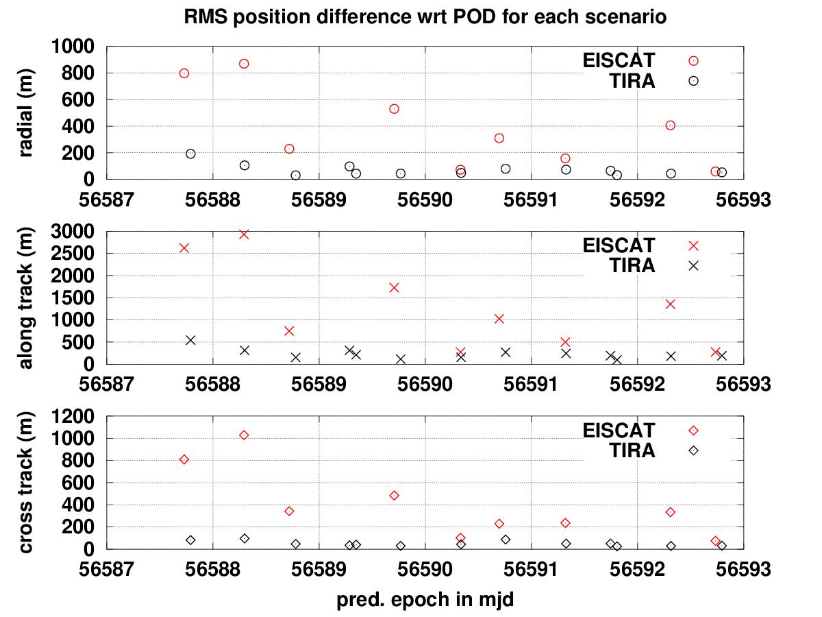
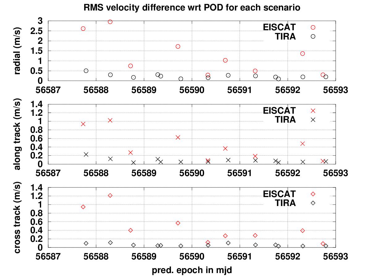
Figure 14: RMS of position (left) and velocity (right) differences w.r.t. POD for each TIRA and EISCAT-based prediction scenario.

4.2.2 Errors in RTW vs errors in Keplerian

On the contrary, if we consider the errors with respect to POD in Keplerian elements (osculating), the larger correlations between the elements are between argument of perigee $\omega$ and mean anomaly $M$ ($>0.99$), but this is due to the low eccentricity of the orbit, and sometimes between the inclination $i$ and the longitude of the ascending node $\Omega$. The correlations between semimajor axis $a$, eccentricity $e$ and mean argument of latitude $\omega+M$ are generally low ($<0.5$). The comparison between the errors in keplerian elements with respect to POD for the first prediction scenarios are shown in Figure 15. We can notice that the errors in semimajor axis are very much aligned between the two sensors. If we want to understand how these input errors affect the propagated re-entry time we can set up a simplified computation.

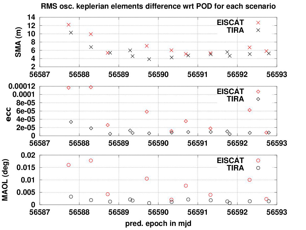
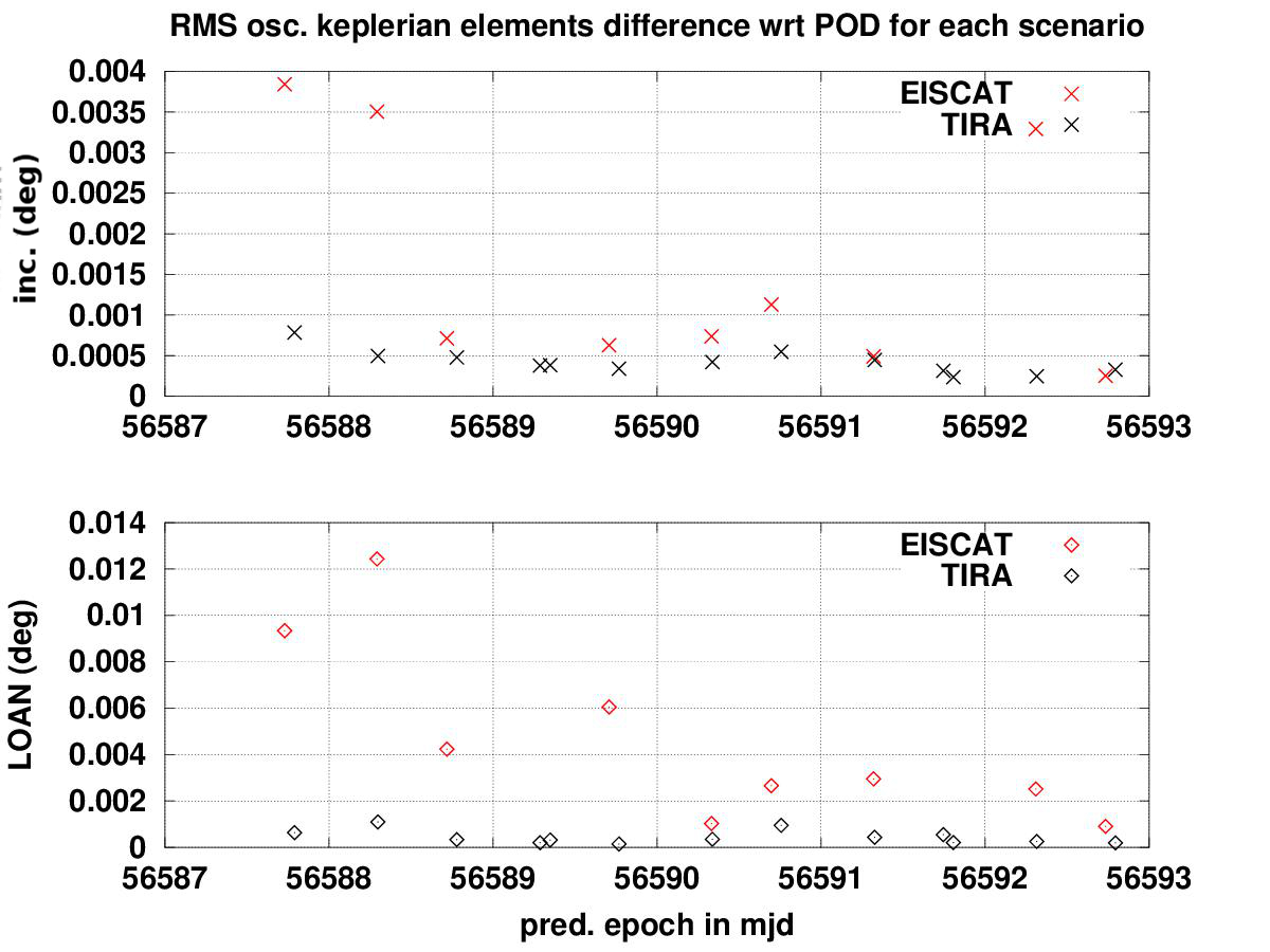
Figure 15: RMS of osculating keplerian elements differences w.r.t. POD for each TIRA and EISCAT-based prediction scenario (left: $a$,$e$,$\omega+M$, right: $i$,$\Omega$).

4.2.3 Variation of re-entry time

We want to set up a simplified computation that gives us a quantification of the variation of the computed re-entry time in function of the initial conditions errors, in Keplerian elements. For this test, we fix the epoch of prediction on Oct-25 (MJD 56590, Table 9), and we let the initial orbital elements to vary inside an interval. With the nominal initial conditions and a $C_{d}A=3.4$m², the nominal re-entry epoch is on Nov-11 at 7:49:48UTC. The size of the variations for each elements are taken from Figures 8, 12 for the corresponding five elements $a$, $e$, $i$, $\Omega$, $\omega+M$, and increased by a conservative factor. Then, for each initial condition a re-entry time is computed, and the final variation can be evaluated.

Table 9: TLE GOCE osculating keplerian elements on 2013-10-25 at 10:54:45 UTC, in GCRS.

$a$	$e$	$i$	$\Omega$	$\omega$	$M$
$6587.553$km	$1.3871\times 10^{-3}$	$96.5163^{\circ}$	$327.5510^{\circ}$	$334.0914^{\circ}$	$134.4271^{\circ}$

Table 10: Simplified test to check the variation of the re-entry epoch prediction w.r.t. the initial conditions variations.

Initial element	Variation interval	Corresponding variation of residual lifetime
		(percentual relative error)
$a$	$\pm 300$m	$<1.0\%$
$e$	$\pm 3\times 10^{-4}$	$<0.5\%$
$\omega+M$	$\pm 0.1^{\circ}$	$<0.5\%$
$i$	$\pm 0.01^{\circ}$	$<0.01\%$
$\Omega$	$\pm 0.05^{\circ}$	$<0.01\%$

What we can see from the results of Table 10 is that both TIRA and EISCAT radar-based orbit determination solutions provide errors that do not change significantly the predicted re-entry epoch. Similar results hold also for a prediction epoch closer to re-entry (e.g. on MJD 56605).

4.2.4 Choice of the calibration time span

As regards the ballistic coefficient estimation, we can apply a similar analysis from the results shown in Figures 9 and 13. In a RMS sense, the variations of the ballistic coefficient estimation are of the order of 1-2% with respect to the nominal value given by the average of the POD-based 30min PWC coefficient. Analogous computations show that the variation of the ballistic coefficient affects the corresponding variation in the predicted re-entry lifetime approximately by the same percentual value, thus implying that the errors in the re-entry predictions shown in Figures 9 and 13, which are of the order of 10%, are not mainly due to OD inefficiencies, but they are dominated by the average mis-modelings occurring in the time span from the prediction epoch to the actual re-entry. For example, they can be due to unpredicted significant attitude changes and unmodeled atmospheric density variations. Strictly speaking, we can say that these re-entry predictions are quite precise but not very accurate (low trueness).

We can see from Figures 6 and 10 (and similars in the next Sections 5 and 6) that the choice of the observation time span is crucial to reconstruct the main variations of the ballistic coefficient. As a matter of fact, for a fixed prediction epoch, different calibration time spans can lead to different ballistic coefficients (they capture the average over a different time span) and thus to different re-entry predictions. At this point, the problem is not to understand if one calibration gives a better prediction than the other, because we know that the correctness of the prediction mostly depend on what happens after the prediction epoch. The main problem is to understand, from what we know from the calibrations up to the current one, what is the general attitude behaviour of the object (e.g. stable, tumbling) and try, if possible, to predict if major changes can occur afterwards. The same applies to the prediction of significant space weather events, and the atmospheric environment variations. However, this can be quite difficult.

The results for the cases analysed in this study indicate that, during the last weeks of decay, intervals of $\sim$36-48h are good enough to reconstruct the average behavior of the ballistic coefficient variations. In general, it is recommended to perform ballistic coefficient calibrations over different time spans, when this is possible, provided that we have enough data avaliable.

In the next Section 5 we will perform the same kind of OD and ballistic coefficient calibration analysis by using TLE data only.

4.3 Critical cases

We have pointed out many times that there are some critical cases for which the standard OD and ballistic calibration does not work properly. First of all, if we have less than four very short tracks from EISCAT, of range and range-rate, the solutions are in general bad determined (or even ill-posed). Second, if we are performing OD close to re-entry, even if we have enough observational data to compute a full solution and good initial conditions, in some cases the dynamical systematic errors are particularly strong to introduce instabilities in the differential corrections and even divergence. This problem can occur for TIRA data processing as well, for instance when we try to fit all the last five TIRA passes together (time span $\sim$48h). We discuss in the following some techniques that can help when dealing with these cases.

1. Only two EISCAT passes. When only two EISCAT passes are available, such as for example the last two tracks shown in Figure 4, a good option would be to ask for the additional availability of a TIRA tracking pass, for example the last one. The significant amount of information contained in the TIRA pass, combined with the two EISCAT pass and a good initial condition (e.g. TLE-based), will lead to a more stable problem and possibly to a good OD and ballistic coefficient estimation. If an additional TIRA pass is not available, but at least the initial condition has a reliable error estimation, then imposing an apriori constraint on the initial position and velocity will lead to a more stable problem and possibly to a good OD and ballistic coefficient estimation. For example, in the cases considered in our tests, if the initial condition is a TLE at an epoch close to the observations times, an empirically derived $\sim$1km constraint in position and $\sim$1m/s in velocity turned out to be a reasonable and effective option.

2. Only three EISCAT passes. The case with three EISCAT passes is quite similar to the previous one, and it can be treated in the same way. However, so far we have considered only range and range-rate short tracks, without assuming any information available for the azimuth and elevation angles of the tracked object. If confirmed, a quite low accuracy information could be deduced from the radar pointing direction, for example to the $1-2^{\circ}$ level. Adding this information on the direction of the tracked object would help in stabilizing the problem and possibly lead to a good OD and ballistic coefficient estimation.

3. Unstable differential corrections. We have always pointed out that, when we approach the re-entry, the altitude decreases and the mis-modelings in the non gravitational perturbations grow in magnitude causing large errors in the estimated orbits. In general we have seen that, given a proper observational scenario, it is possible to find a good solution for re-entry predictions anyway, at the cost of obtaining large residuals with respect to observational noise.

In some cases, even if we have enough observational data, and good initial conditions, it is difficult to compute a full OD and ballistic coefficient estimation because the problem shows instabilities, and the differential corrections diverge. This is the analogous of “over-shooting” effects in the framework of Newton’s method for finding the roots of a generic non linear function. We believe that this problem is mainly due to a combined effect of intrinsic, even small, weaknesses in the OD covariance matrix, and particularly large systematic dynamical errors that affect the residuals. In other words, an analogous observational scenario in presence of lower systematic errors would firmly converge to a good solution. A typical example is the data processing of the last five TIRA observational passes, or the last four EISCAT tracks, which cover $\sim$48h from 2013-Nov-9 to 2013-Nov-10.

We have tried at least three experimental strategies that could help in leading the problem to converge, or at least to approach to a good solution:

• damped differential corrections (under-relaxation),

• differential corrections with pseudoinversion (descoping),

• use of a-priori constraints on initial conditions with deweighed observations.

The first one is recommended when we believe that the observations are enough to have a well-posed OD problem, while the other two are more useful when we have more intrinsic weaknesses in the OD problem. We now briefly describe how these strategies can be applied, to give an idea on what are the main formulas involved. However, this description is not intended to be a guarantee of success in finding always a good solution, and may need a more rigorous treatise to be generalized.

If we generically indicate with $\mathbf{x}$ the 7-dimensional vector of solve for parameters (6-dim state vector + 1 ballistic coefficient), with $B_{x}$ the partial derivatives of the measurements residuals $\mathbf{\xi}$ with respect to $\mathbf{x}$, and with W the weight matrix of the observations, then the normal equations to be solved during the batch least squares differential corrections at iteration $k$ are: $C\Delta\mathbf{x}=\mathbf{D}$, where $\Delta\mathbf{x}=\mathbf{x}_{k}-\mathbf{x}_{k-1}$, $C=B_{x}^{T}WB_{x}$ is the normal matrix, and $\mathbf{D}=-B_{x}^{T}W\xi$. The solution is found by inverting the normal matrix $\Gamma=C^{-1}$, and computing $\Delta\mathbf{x}=\Gamma\mathbf{D}$. More specifically, the inverse matrix can be found by the diaginalization of $C$ with a orthonormal base of eigenvectors: $C=U^{T}EU$, $\Gamma=UE^{-1}U^{T}$, where $U$ is an orthonormal matrix having the eigenvectors of $C$ as columns, and $E$ is a diagonal matrix having the eigenvalues of $C$ as elements. According to (Milani & Gronchi, 2010, Chap.6), given a proper choice of the units of measure, if the confidence ellipsoid defined by $C$ is very much elongated along a particular direction, this direction is given by the eigenvector corresponding to the smallest eigenvalue and is called weak direction. Since, during the differential correction steps, the component of $\Delta\mathbf{x}$ along each eigenvector is multiplied by the inverse of the corresponding eigenvalue, it may happen that the correction along the weak direction is so large to keep the state $\mathbf{x}$ far from the convergence basin.

The main idea here is to force the process to avoid large differential corrections, and check if this succeeds in finding a minimum of the least squares target function. Then such a solution is compared with the reference orbit as usual, to see if it is good enough for a re-entry prediction.

3.1 Damped differential corrections. In this case the idea is to apply a damping factor to the entire correction vector: $\Delta\mathbf{x}=\Gamma\mathbf{D}/\alpha$, where $\alpha=MAX(1,n-k+1)$, $k$ is the current iteration, and $n$ is the number of damped corrections. This process can be iterated, i.e. after $n$ damped corrections we can restart from the current state and compute $n$ new damped corrections. This technique is a type of under-relaxation method for the differential corrections iterative process, with $1/\alpha$ is the under-relaxation factor.

3.2 Differential corrections with pseudoinversion. If $\lambda_{j}$ are the eigenvalues of $C$, in increasing order of magnitude, and $\mathbf{v}_{j}$ are the corresponding eigenvectors, then the differential correction can be also written as $\Delta\mathbf{x}=\sum_{j}\lambda_{j}^{-1}(\mathbf{v}_{j}\cdot\mathbf{D})\mathbf{v}_{j}$. In order to avoid large corrections along the weak direction $\mathbf{v}_{1}$, the pseudoinverse technique consists in relpacing $\lambda_{1}^{-1}=0$ in the $E^{-1}$ matrix, thus $\Delta\mathbf{x}=\sum_{j>1}\lambda_{j}^{-1}(\mathbf{v}_{j}\cdot\mathbf{D})\mathbf{v}_{j}$, and the correction is performed in the hyperplane orthogonal to $\mathbf{v}_{1}$ (see also (Milani & Gronchi, 2010, Chap.10)). The same strategy can be applied on more eigenvalues/eigenvectors, restricting the corrections to lower dimensional hyperplanes.

3.3 A priori constraints on initial conditions with deweighed observations. Another differential correction strategy which could help in finding a good solution in a critical case consists in exploiting an apriori contraint on the initial conditions, such as the one introduced for the cases of only two or three EISCAT tracks. However, what happens here is that the formal covariance matrix $\Gamma$ has already small diagonal terms, because the problem is due to the systematic dynamical errors. To let the apriori constraint help in finding a solution, it is possible to try a uniform deweigh of the observations, i.e. $W\rightarrow W/\beta^{2}$, where $\beta$ is a suitable tuning parameter. One possibility is to choose $\beta$ in order to have the diagonal terms of $\Gamma$ at the same order of magnitude of the a priori constraint variances.

5 TLE-based ballistic coefficient calibration

Exploiting TLE information to calibrate re-entry predictions is a common approach. Adopting the same stretegy described in the previous Section 4, we could use all the TLE available during the three weeks of the GOCE re-entry to perform a piece-wise ballistic coefficient calibration to be compared with the POD-based one.

The procedure simply consists in taking all the TLE available over time intervals of 1-2 days, and perform a full OD and ballistic coefficient estimation by using the TLEs as state observations (i.e. TLE-fitting). The weights to be applied to each TLE’s position and velocity in the fit would need a general knowledge of the accuracy/covariance of its corresponding estimation. Such information is not officially available, and in these experiments we have applied a general data weighing of 1km in position and 1m/s in velocity. The results are shown in Figure 16. As described in Figures 6, 9 for the TIRA calibrations, and Figures 10, 13 for the EISCAT calibrations, also in the TLE-based case the average value of the 30min PWC ballistic coefficient is reconstructed quite well, consistently below the 3% level (computed over each calibration time span).

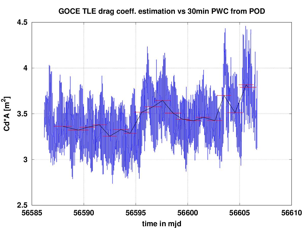
Figure 16: GOCE TLE-based ballistic coefficient estimation over intervals of  36 hours (in red), compared with 30min PWC coefficient from POD (in blue).

2012-006K AVUM R/B

The same experiment can be performed for the 2012-006K AVUM rocket body, and it can be compared with the results computed with the real data given in Section 3. The results are shown in Figures 17 and 18.

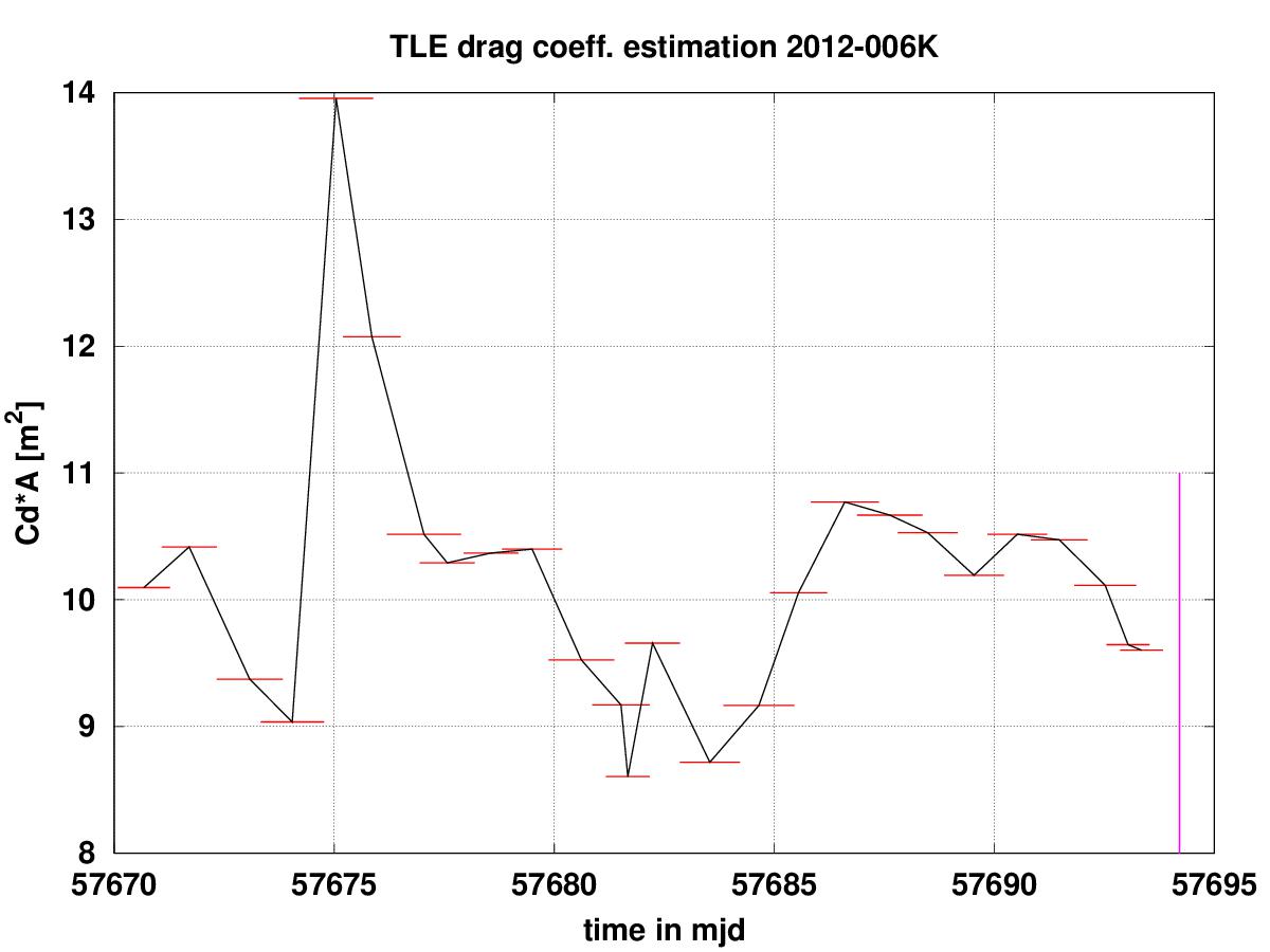
Figure 17: 2012-006K TLE-based ballistic coefficient estimation (in red), over intervals of $\sim$36h. In magenta the nominal re-entry epoch.

As we can recognize in Figure 18, the TIRA/EISCAT-based calibration are in good agreement with the general behavior of the ballistic coefficient variations around their epoch of prediction.

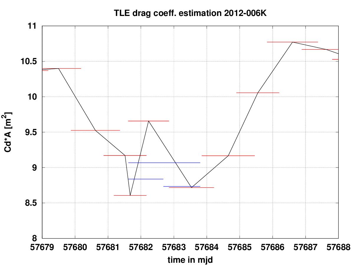
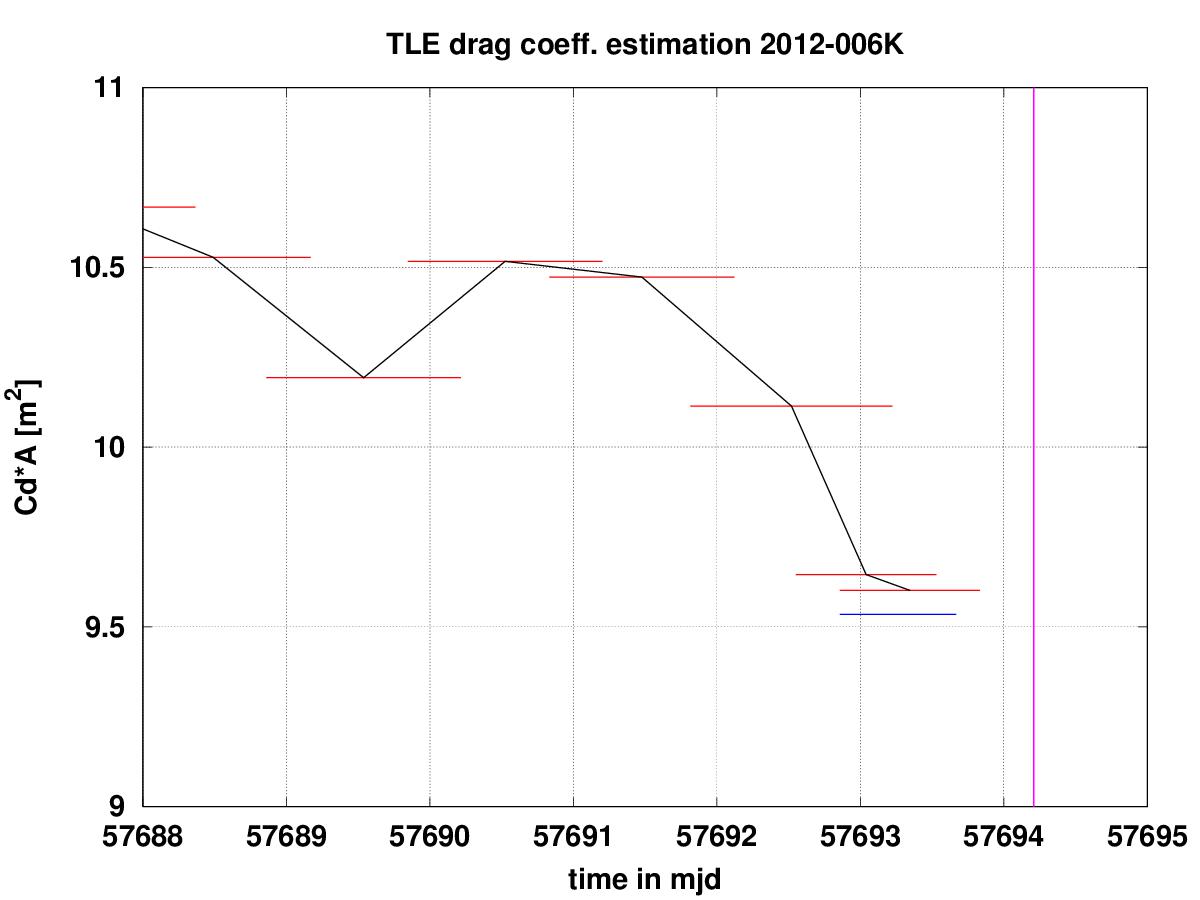
Figure 18: 2012-006K TLE-based ballistic coefficient estimation (in red), over intervals of $\sim$36h. Left: In blue, the radar-based calibrations described in Table 4. Right: In blue, the radar-based calibration described in Table 6.

6 Additional simulations with different types of objects

In order to do a first step in the generalization of the previous analysis, we want to perform EISCAT-based ballistic coefficient calibration also for the simulated objects discussed in Cicalò et al. (2017), which are a spherical and a cylindrical object.

6.1 Sphere

The first object we consider is one with a constant ballistic coefficient. We generated the orbital motion of a sphere-like object that stays close to GOCE quite enough, in order to obtain the same visibility conditions (as in Figure 4). This simulated object has a re-entry at 90km on NOV-11$\sim$00:45 UTC. The useful aspect of the spherical object is that we do not have uncertainties in its cross sectional area or attitude motion, hence we can test the effects due to different atmospheric models. To this purpose, we simulated the reference orbit with a Jacchia-Bowman 2008 density model, and to test the behaviour of a 30min PWC drag coefficient estimation with the NRLMSISE00 density model. As regards the OD tests, also in this case we have considered sets of four subsequent EISCAT tracks. We already stressed that the radar-based orbit determination always tries to capture the average of this function, and this is confirmed also in this case, see Figure 19. Due to the lack of attitude variations, in this simplified test the average value of the ballistic coefficient is very stable, even if large short-term oscillations due to simulated atmospheric density errors are present.

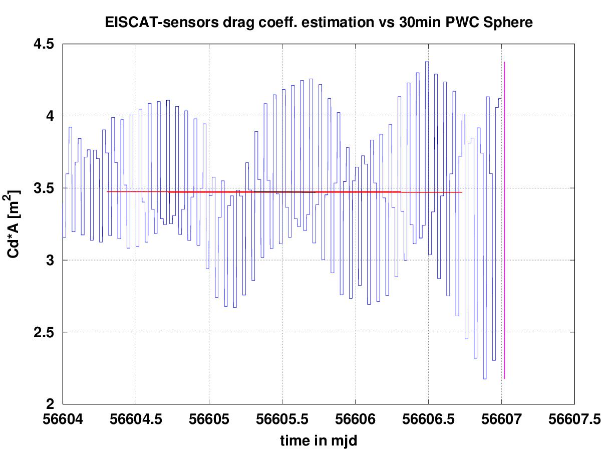
Figure 19: EISCAT-based ballistic coefficient calibration of a sphere-like object (in red), compared with 30min PWC coefficient based on reference orbit (in blue).

6.2 Tumbling cylinder

The tumbling cylinder object is an essentially unoriented cylinder, it has a small centre of gravity offset of $-0.03$m in order to establish tumbling motion within the re-entry period, whose orbit was generated by Belstead Research Ltd. 6DOF propagator (see also Cicalò et al. (2017)). It has the same size of GOCE, and it is propagated from the same initial conditions of GOCE on OCT-22. It has a re-entry at 90km on OCT-27$\sim$23:52UTC. The atmospheric density model used in the simulator for the orbit generation is a dynamic Jacchia-Roberts. In this case, the tumbling increases the average cross-section of the object exposed to drag, thus the absolute magnitude of the ballistic coefficient increases. However, the overall tumbling motion turned out to have a quite stable average value, and we can see in Figure 20 that this is well captured by the radar-based calibrations.

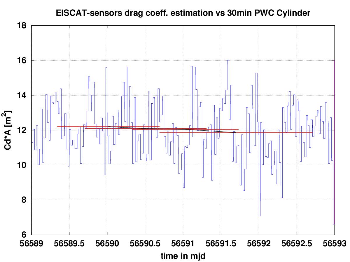
Figure 20: EISCAT-based ballistic coefficient calibration of a tumbling cylinder object (in red), compared with 30min PWC coefficient based on reference orbit (in blue).

6.3 Tumbling cylinder with final stabilization

Finally, the third object that we analyse is an oriented-unstable cylinder, it is a cylinder with a forward centre of gravity of $+0.32$m, which will give it a favoured orientation, but starting from an initial unstable, backward orientation. The result is a vehicle which tumbles, but aligns in the final two days. It is propagated from the same initial conditions of GOCE on OCT-22. The tumbling motion significantly raises the average drag leading to a shorter trajectory, and it has indeed a re-entry at 90km on OCT-28$\sim$1:50UTC.

Since the object tends to align in the final two days, a significant descrease in the long-term average value is expected in the last part of decay. This can be noted in Figure 21, where the EISCAT-based calibrations are effective for the most part of the decay. However, if we are forced to use only four EISCAT pass per calibration, unfortunately in this case we are not able to detect the last $\sim$48h decrease in the ballistic coefficient average value. As discussed before, the addition of just one TIRA pass, if available, during the last day of decay can allow for a shorter-term calibration.

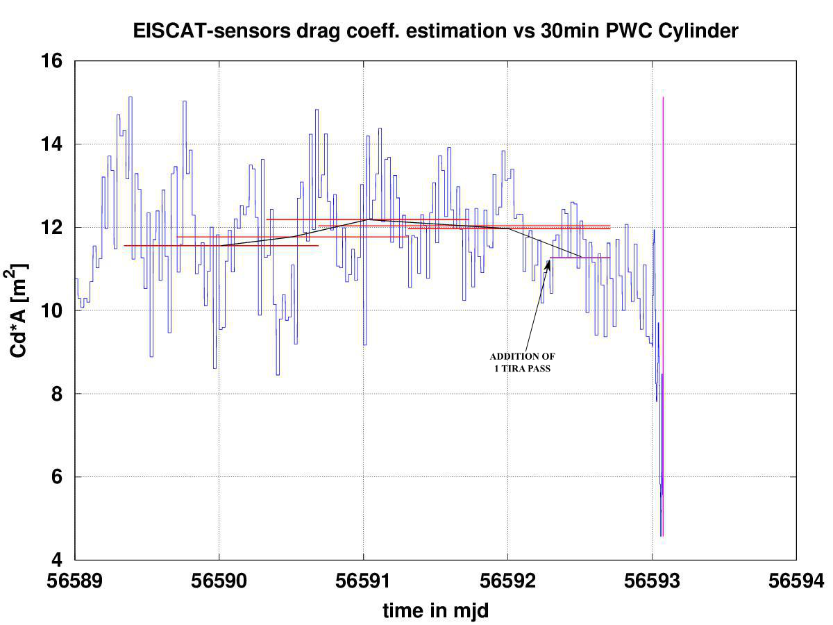
Figure 21: EISCAT-based ballistic coefficient calibration of a tumbling cylinder object with final attitude stabilization (in red), compared with 30min PWC coefficient based on reference orbit (in blue). In the last day of decay an additional TIRA pass is used for a short-time calibration.

7 Conclusions

During this work we have carried out additional analysis on radar-based re-entry prediction calibrations for GOCE, and for other similar decaying objects on circular and highly inclinated orbits. After the analysis described in Cicalò et al. (2017), where the main focus was on the german TIRA radar, we focused here on the northern european sensor EISCAT UHF radar, located in Tromsø, Norway. This sensor, originally conceived for atmospheric studies of the ionosphere, has been recently considered for space debris applications, and in particular for tracking of specific targets, and to support re-entry predictions. The limited tracking capabilities of this sensor posed the problem of establishing to which extent it would be useful to support orbit determination and re-entry predictions, in comparison to what we know about TIRA-like standard prediction calibrations.

By exploiting the large amount of information coming from the re-entry of GOCE, for instance the GPS-based POD and a refined piecewise constant estimation of its ballistic coefficient variations, during the three weeks of uncontrolled decay, we have set up a realistic simulation scenario for a re-entry campaign. Radar-based re-entry predictions and ballistic coefficient calibrations were performed and compared in the cases of TIRA-only, EISCAT-only, and both radar availability situations. The results were compared in terms of differences in the orbital states over the total observation time span, differences in the ballistic coefficient estimation, and in the corresponding re-entry epoch. The main conclusion is that, provided a minimum amount of necessary observational information, EISCAT-based re-entry predictions are of comparable accuracy to TIRA-based (but also to GPS-based, and TLE-based if TLE errors are properly accounted) corresponding ones. Even if the worse tracking capabilities of the EISCAT sensor are not able to determine an orbit at the same level of accuracy of the TIRA radar, it turned out that the estimated orbits are anyway equivalent in terms of re-entry predictions, if we consider the relevant parameters involved and their effects on the re-entry time. What happens to be very important is the difficulty in predicting both atmospheric and attitude significant variations in between the current epoch of observation and the actual re-entry. For completeness, a corresponding GOCE ballistic coefficient estimation based on TLE only was presented, and it turned out to be very effective as well. Some critical cases which consist in a minimum amount of observational information, or in difficulties in obtaining OD convergence, were presented, and a list of possible countermeasures was proposed.

An experiment with real EISCAT (and TIRA) measurements was also presented, for the case of 2012-006K AVUM R/B, which re-entered on 2016-Nov-2. A corresponding TLE-based ballistic coefficient calibration was performed for comparison. The results turned out to be reliable and compatible with each other. Finally, some numerical experiments with simulated trajectories were presented, for the cases of a spherical object, and a cylindrical tumbling object. In both cases we have confirmed the same kind of conclusions obtained for the GOCE case, with an effective estimation of the average behaviour of the ballistic coefficient during the decay phase, with EISCAT data only and EISCAT plus TIRA data available.

In conclusion, from an orbit determination point of view, provided a suitable and reasonable minimum amount of observational data, and of corresponding accuracy information, it is possible to compute reliable and quite precise re-entry predictions. On the contrary, from a more general point of view, the absolute accuracy of each prediction is very much affected by the difficulties in predicting future atmospheric enviroment variations, and significant attitude changes. For this reason, it is not easy to keep the actual accuracy of the predictions much lower than 10% of the residual lifetime, apart from particular cases with constant area to mass ratio, and low atmospheric environment variations with respect to current models.

Future activities on this topic could include at least analogous analysis for objects in more eccentric orbits, and/or with different shapes and attitude behaviours.

References

References

- Bastida Virgili et al. (2014) Bastida Virgili, B., Flohrer, T., Lemmens, S., et al., GOCE Re-entry Campaign, Proceedings of the 5th international GOCE user workshop, ESA Publications Division, European Space Agency, Noordwijk, The Netherlands, 2014.
- Cicalò et al. (2017) Cicalò, S., Beck, J., Minisci, E., et al., GOCE radar-based Orbit Determination for Re-Entry Predictions and comparison with GPS-based POD, proceedings from 7th European Conference on Space Debris, 18-21 April 2017, Darmstadt, Germany.
- Gini et al. (2014) Gini, F., Otten, M., Springer, T., et al., Precise Orbit Determination for the GOCE Re-Entry Phase, Proceedings of the fifth international GOCE user workshop, ESA Publications Division, European Space Agency, Noordwijk, The Netherlands, 2014.
- Lemmens et al. (2014) Lemmens, S., Bastida Virgili, B., Flohrer, T., et al., Calibration of Radar Based Re-entry Predictions, Proceedings of the fifth international GOCE user workshop, ESA Publications Division, European Space Agency, Noordwijk, The Netherlands, 2014.
- Markkanen et al. (2013) Markkanen, J., Nygrén, T., Markkanen, M., Voiculescu, M., and Aikio, A., High-precision measurement of satellite range and velocity using the EISCAT radar, Ann.Geophys., 31, 859-870, 2013.
- Milani & Gronchi (2010) Milani A., Gronchi G.F., Theory of orbit determination, Cambridge University Press, 2010.
- Montenbruck & Gill (2005) Montenbruck, O., Gill, E., Satellite Orbits, Springer-Verlag Berlin Heidelberg, 2005.
- Nygrén et al. (2012) Nygrén, T., Markkanen, J., Aikio, A., and Voiculescu, M., High-precision measurement of satellite velocity using the EISCAT radar, Ann.Geophys., 30, 1555-1565, 2012.
- Pardini et al. (2004) Pardini, C., Tobiska, W.K., Anselmo L., Analysis of the orbital decay of spherical satellites using different solar flux proxies and atmospheric density models, Adv. in Sp.R. 37, 392-400, 2006.
- Vierinen & Krag (2017) Vierinen, J., and Krag, H., Acquisition of radar observations in support for the SST end-to-end validation and technology development, SSA P2-SST-II - SST Radar Observation Executive Summary, March 2017.