Resonances in small scatterers with impedance boundary

Abstract

With analytical (generalized Mie scattering) and numerical (integral-equation-based) considerations we show the existence of strong resonances in the scattering response of small spheres with lossless impedance boundary. With increasing size, these multipolar resonances are damped and shifted with respect to the magnitude of the surface impedance. The electric-type resonances are inductive and magnetic ones capacitive. Interestingly, these subwavelength resonances resemble plasmonic resonances in small negative-permittivity scatterers and dielectric resonances in small high-permittivity scatterers. The fundamental dipolar mode is also analyzed from the point of view of surface currents and the effect of the change of the shape into a non-spherical geometry.

Slight perturbations in a system lead usually to small changes in its response function. In electromagnetic scattering, a good example is Rayleigh scattering which means that the total scattered power of a particle small compared with the wavelength is proportional to the sixth power of its linear size, and thus vanishes predictably for tiny objects. But there are exceptions: a plasmonic subwavelength particle may have a very strong scattering response. This happens, for example, when the relative permittivity of a sphere hits the value $-2$, and the particle is capable of supporting a localized dipolar-like surface plasmon. The magnitude of the resonance is in practice attenuated by material losses and radiation damping but can in principle reach very large values for spheres with diameter much smaller than the wavelength of the incident radiation. In this letter we report on a similar phenomenon that can be found in other type of small scatterers: our analysis shows that particles with a special type of impedance boundary can have scattering and extinction efficiencies that grow without limit when their size decreases in the subwavelength domain. This phenomenon may have fundamental implications regarding the scattering by optically small objects.

In electromagnetics, a multitude of boundary condition exists that can be classified into different categories Lindell_GenDB . Among those, much-used are the PEC (perfect electric conductor) and PMC (perfect magnetic condutor) boundaries, on which the tangential electric (PEC) or tangential magnetic (PMC) field has to vanish. These conditions are special cases of the impedance boundary condition (IBC) which requires the following relation between the tangential electric $(\mathbf{E}_{t})$ and magnetic $(\mathbf{H}_{t})$ fields:

$$\mathbf{E}_{t}=Z_{s}\mathbf{n}\times\left(\eta_{0}\mathbf{H}_{t}\right)$$ (1)

on the surface with unit normal vector $\mathbf{n}$. The surface impedance is a naked number, having units of free-space impedance $\eta_{0}=\sqrt{\mu_{0}\varepsilon_{0}}$. For the impedance surface to be lossless, $Z_{s}$ has to be purely imaginary (methods, , Section 3.6). A passive (dissipative) surface has positive real part of $Z_{s}$, and correspondingly the negative real part means an active surface.

The history of the IBC concept reaches back to 1940’s Shchukin ; Leontovich when it was introduced in connection with the analysis of radio-wave propagation over ground. The scattering problem involving IBC objects has been treated in some studies in the past (Jackson, , Section 10.4), Glisson but it seems that the fundamental phenomenon of resonance modes in small particles has not received earlier attention. The understanding of such mechanisms in the scattering problem opens up possibilities to tailor structures with desired electromagnetic response. This complements other approaches that exist to engineer the scattering characteristics of material objects, such as metasurface-based manipulations ele ; bilo ; glybo and various principles to reduce visibility, like mantle cloaking Alu .

Let us first compute the interaction of an IBC sphere with incident electromagnetic plane wave in free space. The incident field will be scattered from the sphere, and the scattered field can be expanded in an infinite series of spherical harmonic functions. The expansion coefficients follow from the boundary condition at the impenetrable surface of the sphere. Following mutatis mutandis the classical Lorenz–Mie analysis, we arrive at the electric ($a_{n}$) and magnetic ($b_{n}$) scattering coefficients

$$a_{n} = \frac{x\,\mathrm{j}_{n-1}(x)-n\,\mathrm{j}_{n}(x)+\mathrm{i}Z_{s}\,x\,\mathrm{j}_{n}(x)}{x\,\mathrm{h}_{n-1}^{(1)}(x)-n\,\mathrm{h}_{n}^{(1)}(x)+\mathrm{i}Z_{s}\,x\,\mathrm{h}_{n}^{(1)}(x)}$$ (2)

$$b_{n} = \frac{x\,\mathrm{j}_{n-1}(x)-n\,\mathrm{j}_{n}(x)+(\mathrm{i}/Z_{s})\,x\,\mathrm{j}_{n}(x)}{x\,\mathrm{h}_{n-1}^{(1)}(x)-n\,\mathrm{h}_{n}^{(1)}(x)+(\mathrm{i}/Z_{s})\,x\,\mathrm{h}_{n}^{(1)}(x)}$$ (3)

Here $x=2\pi a/\lambda$ is the size parameter of the sphere with radius $a$, and $\mathrm{j}_{n}$ and $\mathrm{h}_{n}^{(1)}$ are the spherical Bessel and Hankel (of the first kind) functions of order $n$. The convention $\exp(-\mathrm{i}\omega t)$ is applied to map the sinusoidal time-dependence into complex numbers. From these coefficients, the scattering (sca), extinction (ext), and absorption (abs) efficiencies can computed according to the same principle as with classical efficiencies of penetrable spheres (Bohren_Huffman, , Section 4.4):

$$Q_{\mathrm{sca}} = \frac{2}{x^{2}}\sum_{n=1}^{\infty}(2n+1)\left(|a_{n}|^{2}+|b_{n}|^{2}\right)$$ (4)

$$Q_{\mathrm{ext}} = \frac{2}{x^{2}}\sum_{n=1}^{\infty}(2n+1)\mathrm{Re}\left\{a_{n}+b_{n}\right\}$$ (5)

$$Q_{\mathrm{abs}} = Q_{\mathrm{ext}}-Q_{\mathrm{sca}}$$ (6)

The efficiency is a dimensionless figure of merit, e.g., the scattering efficiency is the scattering cross section divided by the geometrical cross section of the particle. The series (4) and (5) converge. The larger the sphere in terms of wavelength, the more terms are needed. We use the Wiscombe criterion for the necessary number of terms ($N_{\mathrm{max}}=x+4\sqrt[3]{x}+2$) to truncate the series Wiscombe .

With this mathematical equipment, we can calculate the scattering and extinction behavior of spheres with arbitrary surface impedance and size. For lossy scatterers ($Z_{s}$ has a non-zero real part), all three efficiencies are different while in the lossless case ($Z_{s}$ is purely imaginary), the absorption efficiency vanishes and $Q_{\mathrm{sca}}=Q_{\mathrm{ext}}$. Following the notation of circuit theory, we write the surface impedance as

$$Z_{s}=R_{s}-\mathrm{i}X_{s}$$ (7)

into the surface resistance $R_{s}$ and surface reactance $X_{s}$. The reactance $X_{s}$ is positive for inductive surfaces, and negative for capacitive. The particularly interesting finding from our studies concerns lossless scatterers for which the surface impedance is $Z_{s}=-\mathrm{i}X_{s}$. We plot the scattering efficiencies of IBC spheres as functions of size parameter $x$ for different values of the surface impedance in Figure 1. Due to the lossless character of the sphere, the scattering efficiency equals the extinction efficiency.

 

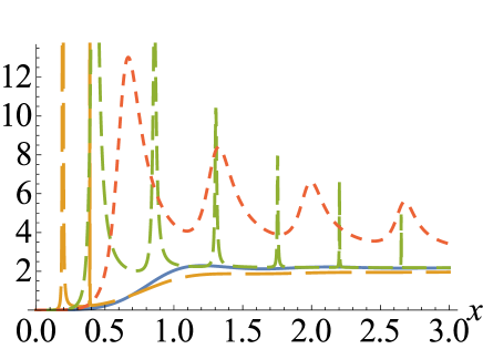
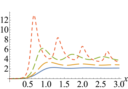
Figure 1: Scattering (extinction) efficiency of lossless impedance spheres as functions of size parameter $x$, for certain values of $X_{s}$ which is the (negative of the) normalized surface reactance: (left) solid blue: $X_{s}=0$ (PEC), long-dashed orange: $X_{s}=-0.2$, short-dashed green: $X_{s}=-0.5$, dotted red: $X_{s}=-1$; (right): solid blue: $X_{s}=\pm\infty$ (PMC), long-dashed orange: $X_{s}=-5$, short-dashed green: $X_{s}=-2$, dotted red: $X_{s}=-1$.

As to their scattering efficiency, the PEC ($Z_{s}=0$) and PMC ($1/Z_{s}=0$) spheres behave identically (the two blue curves in Figure 1). However, the functional form of the responses is far from trivial for intermediate surface impedance values. As the value of the reactance $X_{s}$ decreases from the PMC limit, a gradual increase in scattering amplitude takes place over all the range. The evolution leads to oscillations, and once the surface reactance reaches small (negative) values, the whole curve is dominated by the resonances. In the PEC limit ($X_{s}$ is close to zero), the resonances, riding on top of the gently rolling PEC curve, become vanishingly narrow.

The broadest (dipolar) resonance for very small spheres appears at $-X_{s}\approx x$, and the higher-order modes follow with $-X_{s}\approx x/n$ for integers $n$. Figure 2 shows a closer view the resonances, showing the positions of quadrupolar and octopolar modes for size parameters $x=0.5$ and $x=0.2$. The amplitude of the resonances is $\mathrm{max}\{Q_{\mathrm{sca}}\}\approx 2(2n+1)x^{-2}$, being $24,40,64$ for the three lowest modes in case of $x=0.5$ and $150,250,350$ for $x=0.2$.

 

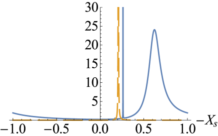
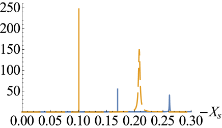
Figure 2: Scattering (extinction) efficiency of lossless impedance spheres as functions of the surface reactance parameter $X_{s}$. The size parameter is $x=0.5$ (solid blue) and $x=0.2$ (long-dashed orange). Due to the broad range of $X_{s}$ in the left-hand side figure, very high-order resonances cannot be distinguished.

Figure 3 illustrates the scattering characteristics as a function of the size parameter and the surface impedance. The effect of increasing sphere size is to soften the resonances and shift their position towards larger values of the imaginary part of the surface impedance. Two clusters of resonance modes exist, one for positive and one for negative $X_{s}$. The resonances at $\mathrm{Im}\{Z_{s}\}>0$ are due to the maxima of the $b_{n}$ Mie coefficients (3), and hence are magnetic type resonances, while the resonances for negative $\mathrm{Im}\{Z_{s}\}$ arise from $a_{n}$ (2), being of electric type. Despite the different visual appearance of the two clusters, they follow the symmetry

$$Q_{\mathrm{sca}}(x,X_{s})=Q_{\mathrm{sca}}(x,-1/X_{s})$$ (8)

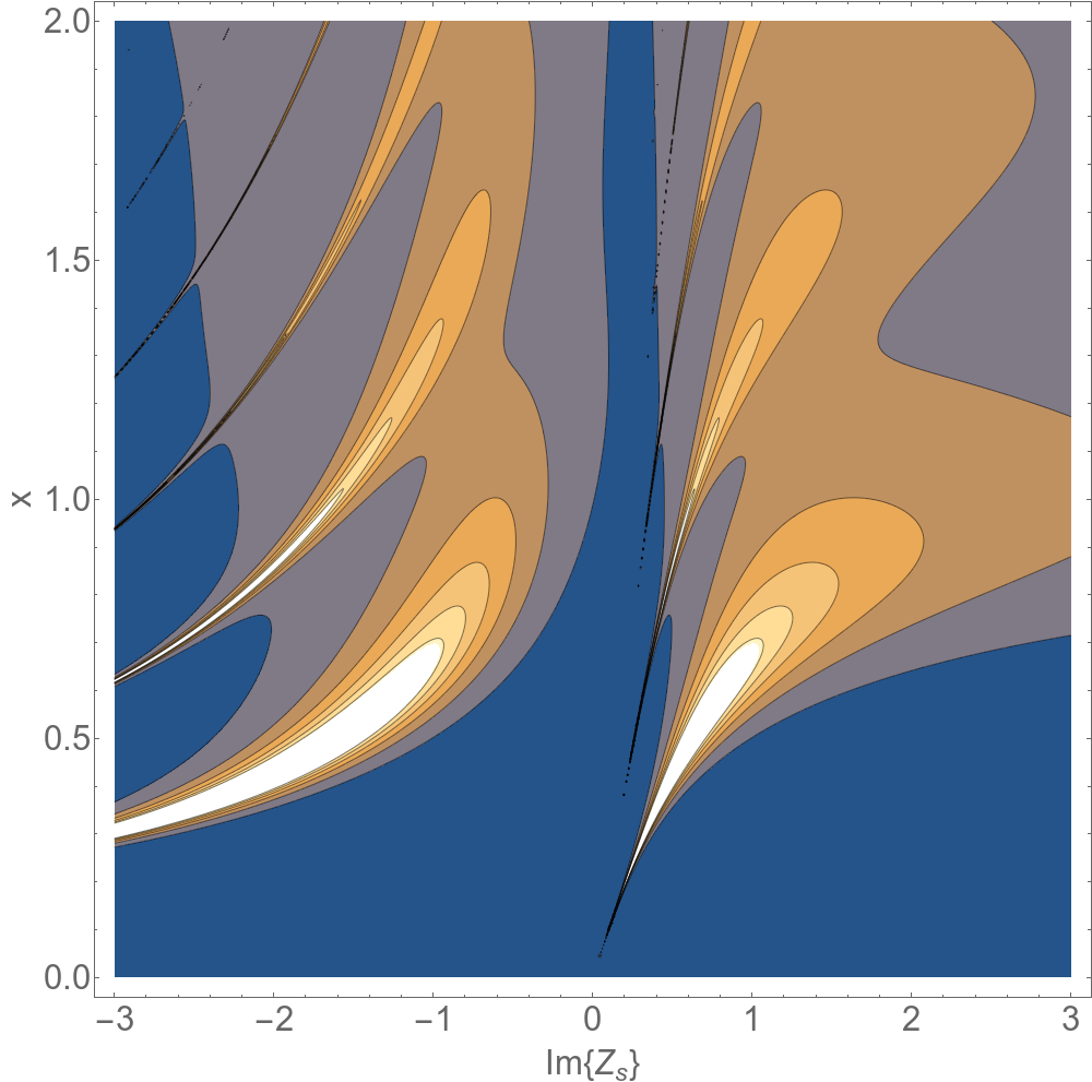
Figure 3: A contour plot of the scattering efficiency of an impedance sphere as function of its surface reactance and the size parameter $x$.

To gain understanding of the mode pattern of the lowest resonance, Figure 4 displays the induced electric $\mathbf{J}_{s}$ and magnetic $\mathbf{M}_{s}$ surface currents on the sphere for the case $x=0.1$ and $Z_{s}=\mathrm{i}\,0.101$, with a plane wave excitation. The surface currents are connected to the tangential fields as $\mathbf{J}_{s}=\mathbf{n}\times\mathbf{H}$ and $\mathbf{M}_{s}=-\mathbf{n}\times\mathbf{E}$. The current distributions show clearly a magnetic dipole type of structure (circulating electric current). Due to the boundary condition (1) where the surface impedance is imaginary, the currents have to be in $90^{\circ}$ phase shifted, and also rotated by $90^{\circ}$ on the sphere surface. The tenfold magnitude of the electric current compared with the magnetic follows from amplitude of the surface reactance. (The figures display only the imaginary(real) part of $\mathbf{J}_{s}$ $(\mathbf{M}_{s})$; the out-of-phase components are around 3000 times smaller.)

 

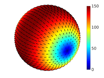
Figure 4: The imaginary part of the electric surface current (left) and the real part of the magnetic surface current (right) for an IBC sphere with size parameter $x=0.1$ and homogeneous scalar surface impedance $Z_{s}=\mathrm{i}\,0.101$. The incident wave is propagating upwards from the bottom.

When the surface impedance $Z_{s}$ has a real part, the surface is no longer lossless. Hence also the three efficiencies in (4)–(6) are different. For passive surfaces (real part of $Z_{s}$ is positive), there is absorption $(Q_{\mathrm{abs}}>0)$, and in case of active surfaces, absorption is negative. The interplay between scattering, absorption, and extinction for lossy impedance spheres is depicted in Figure 5 for two cases: $Z_{s}$ has real and positive values $1$ and $10$.

 

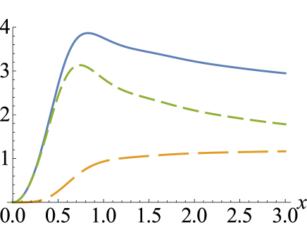
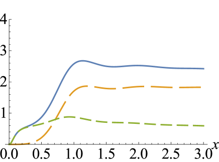
Figure 5: Extinction (solid blue), scattering (long-dashed orange), and absorption (short-dashed green) efficiencies for spheres with lossy surface impedance as a function of the size parameter: $Z_{s}=1$ (left), $Z_{s}=10$ (right).

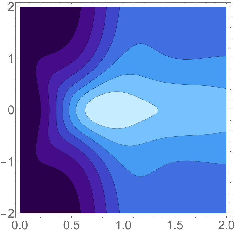
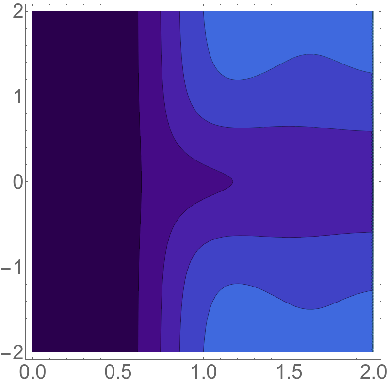
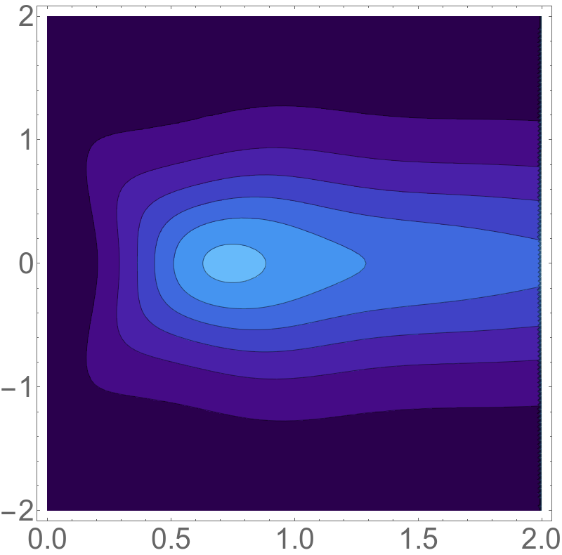
Figure 6: Extinction (left), scattering (center), and absorption (right) efficiencies of a lossy IBC sphere as functions of the size parameter (horizontal axis $x$) and the (logarithmic) surface impedance (vertical axis $a$ with $Z_{s}=10^{a}$).

The dominance of absorption over scattering is conspicuous for small spheres in Figure 5: the extinction is mainly due to absorption when $x$ is small. This phenomenon is also seen in the Taylor expansions of the scattering efficiencies (4) and (5). The ordinary Rayleigh scattering dependence $Q_{\mathrm{sca}}\approx(16/3)x^{4}$ holds for scattering, while the absorption efficiency has a square dependence on the size parameter:

$$Q_{\mathrm{abs}}\approx 6(Z_{s}+1/Z_{s})x^{2}$$ (9)

This square dependence of absorption efficiency on size parameter of IBC spheres differs from the corresponding behavior of the absorption of lossy penetrable dielectric spheres in which the dependence is linear in the small-particle limit rs . For small spheres with fixed $x$, the maximum absorption takes place for increasing $Z_{s}$ or $1/Z_{s}$, but as the size parameter is larger than $0.4$, the maximum is strongest for the “matched-impedance” case $Z_{s}=1$ (for which the scattering achieves its minimum). Such a sphere is an example of a zero-backscattering object ZBO .

The efficiencies are invariant with respect to the change $Z_{s}\rightarrow 1/Z_{s}$. Therefore (8) can be written for general complex IBC spheres as $Q(x,Z_{s})=Q(x,1/Z_{s})$, valid for all three efficiency quantities and $Z_{s}=R_{s}-\mathrm{i}X_{s}$.

Figure 6 shows contour plots of the three efficiencies as functions of the size parameter and the (real-valued) surface impedance. In agreement with the extinction paradox ((Bohren_Huffman, , Section 4.4.3), Brillouin ), the extinction efficiency approaches the value $2$ for large spheres, independent of the surface impedance. The convergence can be slow if $|Z_{s}|\approx 1$: to be within one percent of this limiting value, $x$ needs to be around one thousand.

Sphere is an extravagantly symmetric shape. It is fair to raise the question whether the IBC resonances remain if the spherical symmetry is broken. As an answer we compute the scattering behavior in the vicinity of the resonance of the magnetic dipole for an IBC superspherical object, using numerical surface-integral-equation method based on the electric field integral equation formulation for IBC scatterers eibert ; pasi . The surface of such an object is defined by

$$|x|^{p}+|y|^{p}+|z|^{p}=a^{p}$$ (10)

The value $p=2$ reproduces a sphere with radius $a$, $p=1$ an octahedron, and for increasing $p$, the shape approaches a cube Dimi_josa . Figure 7 shows how the scattering response, in particular how the position of the main resonance shifts with the shape of the object. Not surprisingly, the spherical geometry gives an extremum.

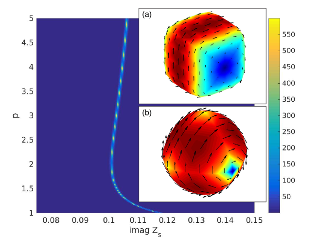
Figure 7: The magnitude of the scattering efficiency of a small lossless IBC quasispherical particle in the plane of the surface impedance and the supersphere parameter $p$. Throughout the $p$ scale, the volume of the particle is the same as the volume of a sphere with $p=2$ for which $x=0.1$. The insets show the electric surface current distributions for cases (a) $p=5$ and (b) $p=1.2$.

The question about material realization of these scatterers remains. In engineering electromagnetics, the boundary condition has been used as an approximation to interfaces between materially strongly contrasting media, often with success, like in the response of metal surfaces in the microwave region. However, interfaces over which the material parameters only change moderately cannot be accurately described by a boundary condition due to the fact that the relation between the tangential electric and magnetic fields depends on the incidence angle and polarization of the incident wave. A remedy to the synthesis problem is the so-called wave-guiding material Lindell06a which is an anisotropic medium that has large components in the permittivity and permeability dyadics in one direction. Cut perpendicular to this direction, the material surface behaves like an impedance surface since the large values of the normally directed material parameter components force the longitudinal fields to vanish, and the fields in the material remain transversal. Adding a parallel metallic plate at a certain depth, the waves are reflected and travel like in a waveguide, and the field relation can be manipulated by varying the transversal permittivity and permeability components of the medium. Another approach to materialize a structure mimicking the surface reactance is to make use of use of frequency-selective-surface (FSS) principles Munk and carve a regular subwavelength pattern of holes on a conducting metallic surface, thus manipulating the ratio between the averaged electric and magnetic fields to produce the desired surface impedance.

References

- (1) I. V. Lindell, A. Sihvola, IEEE Transactions on Antennas and Propagation 65, 4656 (September 2017)
- (2) I. V. Lindell, Methods for Electromagnetic Field Analysis (Oxford University Press and IEEE Press, Oxford, 1992, 1995)
- (3) A. N. Shchukin, Propagation of radio waves (Svyazizdat, Moscow, 1940)
- (4) M. A. Leontovich, Bulletin of Academy of Sciences USSR, Phys. Ser. 8, 16 (1944)
- (5) J. D. Jackson, Classical Electronynamics (John Wiley & Sons, Inc., New York, 1999)
- (6) A. W. Glisson, Radio Science 27, 935 (November–December 1992)
- (7) M. Selvanayagam and G. V. Eleftheriades, Physical Review X 3, 041011 (November 2013)
- (8) S. Vellucci, A. Monti, A. Toscano and F. Bilotti, Physical Review Applied 7, 034032 (March 2017)
- (9) S. B. Glybovski, S. A. Tretyakov, P. A. Belov, Y. S. Kivshar and C. R. Simovski, Physics Reports 634, 1 (2016)
- (10) A. Alù, Physical Review B 80, 241115 (December 2009)
- (11) C. F. Bohren and D. R. Huffman, Absorption and Scattering of Light by Small Particles (John Wiley & Sons, Inc., New York, 1983)
- (12) W. J. Wiscombe, Applied Optics 19, 1505 (May 1980)
- (13) L. Brillouin, Journal of Applied Physics 20, 1110 (November 1949)
- (14) H. Wallén, H. Kettunen and A. Sihvola, Radio Science 50, 18 (January 2015)
- (15) I. V. Lindell A. H. Sihvola, P. Ylä-Oijala and H. Wallén, IEEE Transactions on Antennas and Propagation 57, 2725 (September 2009)
- (16) Ismatullah and T. F. Eibert, IEEE Transactions on Antennas and Propagation 57, 2084 (July 2009)
- (17) P. Ylä-Oijala, J. Lappalainen and S. Järvenpää, IEEE Transactions on Antennas and Propagation 66, 487 (January 2018)
- (18) D. C. Tzarouchis, P. Ylä-Oijala, T. Ala-Nissila and A. Sihvola, Journal of the Optical Society of America B 33, 2626 (December 2016)
- (19) I. V. Lindell and A. H. Sihvola, IEEE Transactions on Antennas and Propagation 54, 3669 (December 2006)
- (20) B. A. Munk, Frequency Selective Surfaces: Theory and Design (John Wiley & Sons, Inc., New York, 2000)