Dynamically integrated transport approach for heavy-ion collisions at high baryon density

Abstract

We develop a new dynamical model for high-energy heavy-ion collisions in the beam energy region of the highest net-baryon densities on the basis of nonequilibrium microscopic transport model JAM and macroscopic (3+1)-dimensional hydrodynamics by utilizing a dynamical initialization method. In this model, dynamical fluidization of a system is controlled by the source terms of the hydrodynamic fields. In addition, time dependent core-corona separation of hot regions is implemented. We show that our new model describes multiplicities and mean transverse mass in heavy-ion collisions within a beam energy region of $3<\sqrt{s_{NN}}<30$ GeV. Good agreement of the beam energy dependence of the $K^{+}/\pi^{+}$ ratio is obtained, which is explained by the fact that a part of the system is not thermalized in our core-corona approach.

I Introduction

The study of the structure of the QCD phase diagram is one of the most important subjects in high-energy heavy-ion physics. Ongoing experiments such as the Relativistic Heavy-Ion Collider (RHIC) Beam Energy Scan (BES) program Adamczyk:2017iwn ; Aggarwal:2010cw ; Kumar:2013cqa and the NA61/SHINE experiment at the Super Proton Synchrotron (SPS) NA61SHINE enable us to explore the high baryon density domain by creating compressed baryonic matter (CBM) in laboratory experiments cbmbook . Future experiments currently planned such as, BES II of STAR at RHIC BESII , the CBM experiment at FAIR FAIR , MPD at NICA, JINR NICA , and a heavy-ion program at J-PARC (J-PARC-HI) HSakoNPA2016 will offer opportunities at the most favorable beam energies to explore the highest baryon density matter. These studies on the high-baryon density matter may also have implications for understanding neutron stars and their mergers through astronomical observations Baym:2017whm . For example, the binary neutron-star mergers TheLIGOScientific:2017qsa are expected to discriminate dense baryonic matter equation of state (EoS) at the densities five to ten times higher than the normal nuclear matter density $\rho\sim(5-10)\rho_{0}$ ($\varepsilon=(0.75-1.5)~{}\mathrm{GeV}/\mathrm{fm}^{3}$) via the gravitational wave spectrum Sekiguchi:2011zd . In heavy-ion collisions, the search for a first-order phase transition and the QCD critical point predicted by some theoretical models DHRischke2004 is one of the most exciting topics.

To extract information from experiments, we need dynamical models for understanding the collision dynamics of heavy-ion collisions. At RHIC and the LHC, the hydrodynamical description of heavy-ion collisions has been successful in explaining a vast body of data, in which hydrodynamical evolution starts at a fixed proper time of about $\tau\sim 1$ fm/$c$ with initial conditions provided by some other theoretical models Heinz:2013th ; Gale:2013da ; Huovinen:2013wma ; Hirano:2012kj ; Jeon:2015dfa ; Jaiswal:2016hex ; Romatschke:2017ejr . Systematic analyses of RHIC and LHC data have been done based on Bayesian statistics using state-of-the-art hybrid simulation codes to extract the quark gluon plasma (QGP) properties  Pratt:2015zsa ; Bernhard:2016tnd . However, this picture breaks down at lower beam energies $\sqrt{s_{NN}}<30$ GeV for the description of heavy-ion collisions since the passing time of two nuclei exceeds 1 fm/$c$ and secondary interactions become important before two nuclei pass through each other. Thus one needs a nonequilibrium transport model to follow dynamics before hydrodynamical evolution starts. We note, however, that as an alternative approach to heavy-ion collisions at baryon stopping region, three fluid dynamics (3FD) has been used extensively to analyze the collision dynamics Brachmann:1997bq ; Ivanov:2005yw ; Ivanov:2013yla ; Batyuk:2016qmb ; Ivanov:2018vpw .

The UrQMD hybrid model has been developed for simulations of heavy-ion collisions at high baryon density Steinheimer:2007iy ; Petersen:2008dd . In this approach, the initial nonequilibrium dynamics of the collision is treated by the UrQMD model, and one assumes that the system thermalizes just after two nuclei pass through each other, then dynamics of the system is followed by hydrodynamics. Finally, after the system becomes dilute, one switches back to UrQMD to follow the time evolution of a dilute hadron gas. It was pointed out that the separation of the high density (core) and the peripheral (corona) part is significant at the top SPS and RHIC energies for the description of centrality dependence of the nuclear collisions Werner:2007bf . As core-corona separation should be also significant at lower beam energies, it has been implemented into a UrQMD hybrid model, which improves the description of the experimental data Steinheimer:2011mp . This approach has been extended by incorporating viscous hydrodynamics Karpenko:2015xea ; Auvinen:2017fjw .

Recently, a dynamical initialization approach has been proposed on the basis of the hydrodynamics with source terms which enable a unified description of energy loss of jets by the bulk hydrodynamic environment at RHIC and LHC energies Okai:2017ofp . A similar idea was applied to develop a new dynamical initialization approach based on string degrees of freedom for the description of heavy-ion collisions at RHIC-BES energies Shen:2017bsr . In this approach, instead of assuming a single thermalization time, hydrodynamical evolution starts at different times locally, so one can simulate a collision of finite extensions of colliding nuclei.

In this paper, we present a new dynamically integrated transport model by combining the JAM transport model and hydrodynamics. We utilize the same idea as Ref. Okai:2017ofp ; Shen:2017bsr for the dynamical initialization of the fluids. At the same time, our approach takes into account the core-corona separation picture both in space and time; hydrodynamical evolution starts at different spacetime points where energy density is sufficiently high. Another distinct feature of our approach from the previous models Okai:2017ofp ; Shen:2017bsr is that spacetime evolution of nonequilibrium part of the system is simultaneously solved by the microscopic transport model together with hydrodynamical evolution.

Most of the hadronic transport models lack multiparticle interactions in the dense phase. Hybrid approaches can overcome this type of defect. An immediate consequence of the improvement is the enhancement of the strange particle yields relative to the predictions by a standard hadronic transport approach, as pointed out in Ref. Petersen:2008dd .

Statistical model predicts the nontrivial structure Gazdzicki:1998vd called “horn” in the excitation function of the $K^{+}/\pi^{+}$ ratio, which was observed in the experiments Afanasiev:2002mx ; Alt:2007aa . The existence of this sharp structure has been explained by several statistical models  Andronic:2005yp ; Andronic:2008gu ; Satarov:2009zx ; Becattini:2003wp ; Becattini:2005xt . On the other hand, hadronic cascade models failed to describe such structures in the ratios Afanasiev:2002mx ; Alt:2007aa even though some models include collective effects such as string fusion to color ropes . However, recently, the parton-hadron-string dynamics (PHSD) transport model reproduced horn structure by the interplay between the effects of chiral symmetry restoration and deconfinement into quark-gluon degrees of freedom Cassing:2015owa . This is the first explanation of the horn from a dynamical approach. In this paper, we shall show that our dynamical approach also describes well the excitation function of the $K^{+}/\pi^{+}$ ratio by taking into account an incomplete thermalization of the system.

This paper is organized as follows: Section II describes our transport approach. Section III presents the results for the excitation function of the mean transverse mass, multiplicities, and particles ratios. The conclusions are given in Sec. IV.

II Dynamical model

We use the JAM transport model JAMorg for the description of nonequilibrium dynamics, which is based on the particle degrees of freedom: hadrons and strings. JAM describes the time evolution of the phase space of $N$ particles by the so-called cascade method. Particle production in JAM is modeled by the excitation and decay of resonances and strings as employed by other transport models RQMD1995 ; UrQMD1 ; UrQMD2 . We use the same string excitation scheme as the HIJING model HIJING , and the Lund model for string fragmentations in PYTHIA6 pythia6 . Secondary products from decays of resonances or strings can interact with each other via binary collisions. A detailed description of the hadronic cross sections and cascade method implemented in the JAM model can be found in Ref. JAMorg ; Hirano:2012yy . In this work, we include neither hadronic mean-field nor modified scattering style in two-body collisions Isse ; Nara:2016phs ; Nara:2016hbg ; Nara:2017qcg , thus particle trajectories in the JAM cascade are straight lines until particles scatter with each other or decay.

We consider a dynamical coupling of the microscopic transport model and macroscopic hydrodynamics. Specifically, the JAM model is coupled with hydrodynamics by source terms $J^{\mu}$ and $\rho$:

$$\partial_{\mu}T_{f}^{\mu\nu}=J^{\nu},~{}~{}\partial_{\mu}N_{f}^{\mu}=\rho,$$ (1)

where $T_{f}^{\mu\nu}$ is the energy-momentum tensor of the fluids. We assume the ideal fluid $T_{f}^{\mu\nu}=(e+p)u^{\mu}u^{\nu}-pg^{\mu\nu}$, where $u^{\mu}$ is the four-fluid velocity, $e$ and $p$ are the local energy density and pressure. Here $N_{f}^{\mu}=nu^{\mu}$ is the baryon current.

In our practical implementation of the source term $J^{\mu}$ and $\rho$, particles are converted into fluid elements when they decay from strings or hadronic resonances and if the local energy density (the sum of the contributions from particles and fluids) at the point of decay exceeds the fluidization energy density $e_{\text{f}}$ in order to ensure the core-corona separation. We use $e_{\text{f}}=0.5$ GeV/fm³ as a default value, which is the same as the particlization energy density $e_{\text{p}}$ introduced later.

One expects that the fluidization energy density $e_{\text{f}}$ must be the same as the particlization energy density $e_{\text{f}}$ in the static equilibrium state. However, $e_{\text{f}}$ may be different from $e_{\text{p}}$ at a highly nonequilibrium state such as occur in the initial stages of heavy-ion collisions. Note that the fluidization condition also depends on the baryon density. The transition energy density to QGP at high baryon densities would be higher than the largest value of 0.5 GeV/fm³ that is obtained by the lattice QCD calculations at vanishing chemical potentials Bazavov:2014pvz . Thus we do not exclude possibilities of higher values of $e_{\text{f}}=0.8$ and 1.0 GeV/fm³.

In the case of string decay, decay products are absorbed into fluids after their formation times with the same criterion as above. Leading particles, which have original constituent quarks from string decay, are not converted into fluids, in order to keep the same baryon stopping power as in the JAM cascade model. Thus, our source terms in which particles are entirely absorbed into fluid elements within a time step $\Delta t$ take the form

$$J^{\mu}(\bm{r}) =\frac{1}{\Delta t}\sum_{i}p^{\mu}_{i}(t)G(\bm{r}-\bm{r}_{i}(t)),$$ (2)

$$\rho(\bm{r}) =\frac{1}{\Delta t}\sum_{i}B_{i}G(\bm{r}-\bm{r}_{i}(t)),$$ (3)

where $B_{i}$ is the baryon number of $i$-th particle, and the sum runs over the particles to be absorbed into fluid elements at the time interval between $t$ and $t+\Delta t$. The Gaussian smearing profile is given by

$$G(\bm{r})=\frac{\gamma}{(2\pi\sigma^{2})^{3/2}}\exp\left(-\frac{\bm{r}^{2}+(\bm{r}\cdot\bm{u})^{2}}{2\sigma^{2}}\right),$$ (4)

where $\bm{u}=\bm{p}/m$ is the velocity of the particle, and $\gamma=p^{0}/m$ Oliinychenko:2015lva , in which the profile is Lorentz contracted to ensure the Lorentz invariance in the combination of $G(\bm{r})d^{3}r$. In this work, we use $\sigma=0.5$ fm.

As we force the thermalization of the system by hand in our approach neglecting viscous effects, there is no way to match all the quantities between particles and fluids. Therefore, we simply assume that the local energy density of the particles is obtained from $T_{p}^{\mu\nu}$ in the Eckart frame defined by $N_{p}^{\mu}$, where the particle currents are calculated as

$$T_{p}^{\mu\nu}(\bm{r}) =\sum_{i}\frac{p_{i}^{\mu}(t)p_{i}^{\nu}(t)}{p^{0}_{i}(t)}G(\bm{r}-\bm{r}_{i}(t)),$$ (5)

$$N_{p}^{\mu}(\bm{r}) =\sum_{i}\frac{p_{i}^{\mu}(t)}{p^{0}_{i}(t)}G(\bm{r}-\bm{r}_{i}(t)),$$ (6)

where the summation runs over all particles, and $p_{i}^{\nu}(t)$ and $\bm{x}_{i}(t)$ are the four-momenta and the coordinates of the $i$-th particle, respectively. We have checked that our final results are unaffected when we instead reconstruct the local energy density from the computational-frame particle energy and momentum using the EoS.

Hydrodynamical equations are solved numerically by employing the Harten–Lax–van Leer–Einfeldt (HLLE) algorithm Schneider:1993gd ; Rischke1 ; Karpenko:2013wva in three spatial dimensions with operator splitting method. There are some modifications from the original implementations Schneider:1993gd ; Rischke1 ; Karpenko:2013wva . First, cell interface values $Q_{\pm}=(\bm{v}_{\pm},e_{\pm},p_{\pm},n_{\pm})$ for the local variables of fluid velocity $\bm{v}$, energy density $e$ and baryon density $n$ are obtained via the monotonized central-difference (MC) limiter VanLeer ; Okamoto:2017ukz instead of using minmod slope limiter. In addition, we take space averages of the linear interpolation function for the cell interface values at each cell boundary. Then, we construct cell interface values for the conserved quantities

$$T^{00}_{\pm} =(e_{\pm}+p_{\pm})\gamma^{2}_{\pm}-p_{\pm},$$ (7)

$$T^{0i}_{\pm} =(e_{\pm}+p_{\pm})\gamma^{2}_{\pm}v^{i}_{\pm},~{}(i=x,y,z)$$ (8)

$$N^{0}_{\pm} =\gamma_{\pm}n_{\pm},$$ (9)

from which we compute numerical flux by using the HLLE algorithm. The cell size of $\Delta x=\Delta y=\Delta z=0.3$ fm, and the time-step size of $\Delta t=0.15$ fm/$c$ are used in the present study.

EoS which covers all baryon chemical potentials $\mu_{B}$ in the QCD phase diagram has not yet been available from lattice QCD calculations. In lattice QCD, EoS at finite baryon densities is usually obtained by the Taylor expansion of the pressure in $\mu_{B}/T$ around $\mu_{B}=0$, and it is extended up to $\mu_{B}\approx 300-400$ MeV Bazavov:2017dus . Since it does not cover all the baryon chemical potential needed for our beam energy regions, we take EoS from phenomenological model calculations in this work. We employ an equation of state, EOS-Q EOSQ , which exhibits a first-order phase transition between massless quark-gluon phase with bag constant $B^{1/4}=235$ MeV and hadronic gas with resonances up to 2 GeV. In the hadronic phase, we include a baryon density dependent single-particle repulsive potential $V(\rho_{B})=K\rho_{B}$ with $K=0.45$ GeVfm³ for baryons. In the present work, all results are obtained by using EOS-Q. We will report EoS dependence on the particle productions in detail elsewhere.

Fluid elements are converted into particles by using the positive part of the Cooper-Frye formula Cooper:1974mv

$$\Delta N_{i}=\frac{g_{i}}{(2\pi)^{3}}\int\frac{d^{3}p}{E}\frac{[\Delta\sigma\cdot p]_{+}}{\exp[(p\cdot u-\mu_{i})/T]\pm 1},$$ (10)

where $[\cdots]_{+}=\theta(\cdots)|\cdots|$, $\Delta\sigma_{\mu}$ is the hypersurface element, and $g_{i}$ and $\mu_{i}$ are the spin degeneracy factor and the chemical potential for $i$th hadron species, respectively. CORNELIUS 1.4 is used to compute freeze-out hypersurface Huovinen:2012is . We use a method similar to that of Ref. Pratt:2014vja for the Monte-Carlo sampling of particles. When potentials are included in the EoS, we use the effective baryon chemical potential in the Cooper-Frye formula

$$\mu^{\text{eff}}_{B}=\mu_{B}-V(\rho_{B})=\mu_{B}-K\rho_{B}$$ (11)

to ensure the smooth transition from fluids to particles. We assume that particlization occurs at the energy density of $e_{\text{p}}=0.5$ GeV/fm³ in the present work.

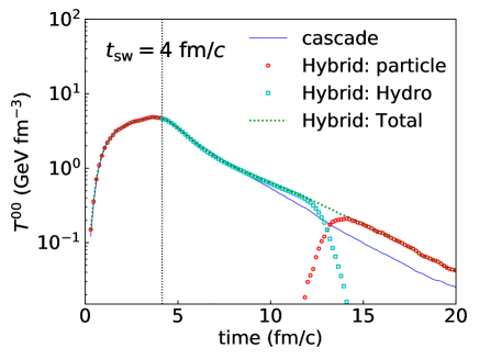
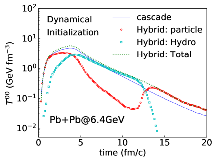
Figure 1: Time evolution of the energy density at the coordinate origin $(x,y,z)=(0,0,0)$ from JAM hybrid simulations with $e_{\text{f}}=e_{\text{p}}=0.5$ GeV/fm³ in central Pb + Pb collisions at $\sqrt{s_{{\scriptscriptstyle NN}}}=6.4$ GeV ($E_{\text{lab}}=20A$ GeV). Upper panel shows the results from calculations by the fixed switching time at $t_{\text{sw}}=4$ fm/$c$. The result from a dynamical initialization is shown in the lower panel. The circles show the contribution from particles, and the squares show the fluid contribution to the energy density.

Let us first examine the time evolutions of the system. In Fig. 1, the time evolutions of the energy density $T^{00}$ at the coordinate origin of central Pb + Pb collisions ($b<3.4$ fm) at $\sqrt{s_{{\scriptscriptstyle NN}}}=6.4$ GeV ($E_{\text{lab}}=20A$ GeV) are shown. The average is taken over about 1000 events. In the upper panel of Fig. 1, the results from the hybrid simulations with a fixed switching time of $t_{\text{sw}}=4$ fm/$c$ are displayed, where the switching time $t_{\text{sw}}=2R/(\gamma v)$ is assumed by the condition that hydrodynamical evolution starts immediately after the two nuclei have passed through each other, where $R$ and $v$ are the radius and the incident velocity of the colliding nuclei, respectively, and $\gamma$ is the Lorentz factor. The circles depict the energy density evolution from particles in JAM, while the squares correspond to the energy density of hydrodynamics. The dotted line is the sum of two contributions. The energy density of the particle contribution is computed by using the Gaussian smearing profile Eq. (5) at the coordinate origin $(x,y,z)=(0,0,0)$, and the energy density of the fluids corresponds to the value of the cell at the origin $T^{00}(0,0,0)$. Until the switching time $t_{\text{sw}}=4$ fm/$c$, time evolution of the energy density is identical to the cascade simulation (solid line) as it should be. After switching to fluids, the expansion of the system becomes slower than that in the cascade simulation. We have found that it is important to include the effects of potential in the Cooper-Frye formula by using e.g., the effective baryon chemical potential Eq. (11) in order to ensure the smooth transition from fluids to particles at the particlization, in case mean-field potential is included in the EoS.

The lower panel of Fig. 1 shows the time evolution of energy density in the case of dynamical initialization. The energy density of particles reaches the maximum value at $t=2.5$ fm/$c$, and the energy density of the fluids gradually increases up to 3 GeV/fm³ at 5 fm/$c$. It is also important to observe that hydrodynamical evolution already starts before two nuclei pass through each other. The sum of energy densities from particles and fluid elements is shown by the dotted line and is larger than the cascade result. The dynamical initialization leads to a very different dynamical evolution of the system compared wiht the simulation with a fixed switching time.

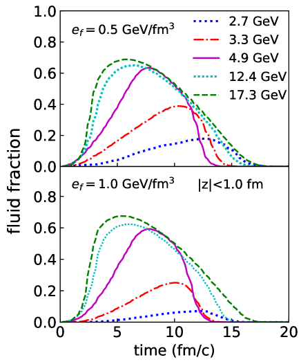
Figure 2: Time evolution of the fractions of the fluid energy for $e_{\text{f}}=0.5$ GeV/fm³ (upper panel) and $e_{\text{f}}=1.0$ GeV/fm³ (lower panel) at the central region $|z|<1.0$ fm from JAM hybrid simulations in central Au + Au at $\sqrt{s_{{\scriptscriptstyle NN}}}=2.7,3.3$, and 4.9 GeV, and Pb + Pb collisions at $\sqrt{s_{{\scriptscriptstyle NN}}}=12.4$ and 17.3 GeV.

Figure 2 shows the time evolution of the fraction of the fluid energy in the central region of $|z|<1$ fm, in which the energy density of the fluid elements is greater than 0.5 GeV/fm³ for central Au + Au and Pb + Pb collisions at $\sqrt{s_{{\scriptscriptstyle NN}}}=2.7,3.3,4.9,12.4$, and 17.3 GeV. The results for the fluidization energy densities $e_{\text{f}}=0.5$ GeV/fm³ and 1.0 GeV/fm³ are shown in the upper panel and the lower panel of Fig. 2, respectively. The fluid fraction increases slowly with time at lower beam energies. As beam energy becomes higher, the fluid fraction increases rapidly, and particle-fluid conversion process becomes close to that in the single thermalization time simulations. The fluid fraction is insensitive to the $e_{\text{f}}$ value for high beam energies, while it is sensitive at lower energies. The fluid fraction at $\sqrt{s_{{\scriptscriptstyle NN}}}=17.3$ GeV reaches about 70% at $t=6$ fm/$c$, which is smaller than the UrQMD hybrid core-corona model Steinheimer:2011mp , in which almost the entire system enters the hydrodynamics at the highest SPS energies in central Pb + Pb collisions. One of the main reasons is that, in our approach, preformed hadrons (hadrons within their formation times) and leading hadrons are not converted into fluids, while in the UrQMD hybrid model, they are included in the hydrodynamical evolution at the switching time, which is necessary for the total energy-momentum conservation. Additionally, in this work, we assume that preformed hadrons are converted into fluids after their formation time, which implies that the formation time of hadrons equals the local thermalization time of the system at dense region. Nevertheless, it would be interesting to investigate the influence of shorter thermalization times on the dynamics in our approach.

III Results

We compare our results from JAM+hydro hybrid model with the results from JAM cascade model and the experimental data in central Au+Au/Pb + Pb collisions. We perform calculations with the impact parameter range $b<4.0$ fm for 7% central Pb + Pb at $\sqrt{s_{{\scriptscriptstyle NN}}}=$6.4–12.4 ($E_{\text{lab}}=20$–$80A$ GeV), and $b<3.4$ fm for 5% central collision for the other collisions.

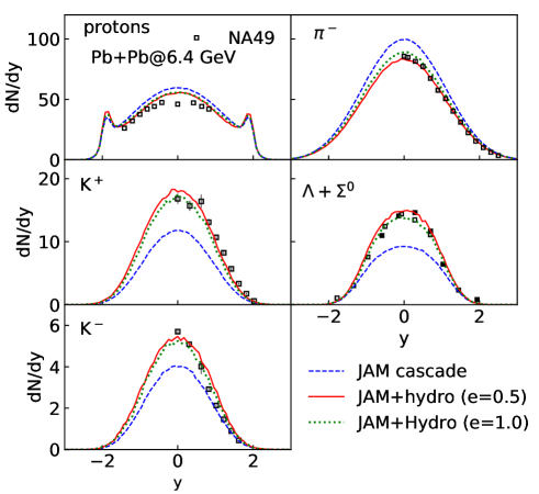
Figure 3: Rapidity distributions of protons, negatively charged pions, negatively and positively charged kaons, and $\Lambda$s in the central Pb + Pb collisions at $\sqrt{s_{{\scriptscriptstyle NN}}}=6.4$ GeV. The results from JAM cascade (dashed lines) and JAM + hydro calculations with $e_{\text{f}}=0.5$ (dotted lines) and 1.0 GeV/fm³ (solid lines) are compared with the experimental data Alt:2007aa ; Alt:2008qm ; Blume:2007kw .

First we compare the results of our approach in central Pb + Pb collisions at $\sqrt{s_{{\scriptscriptstyle NN}}}=6.4$ GeV for the rapidity (Fig. 3) with the NA49 data  Alt:2007aa ; Alt:2008qm ; Blume:2007kw to see the effects of hydrodynamical evolution. We also compare the results from different values of the fluidization energy densities $e_{\text{f}}=0.5$ and 1.0 GeV/fm³. In the hybrid simulations, the rapidity distribution of protons is slightly lower than those in the cascade simulations, and stopping power of two nuclei is similar between hybrid and cascade simulations for both $e_{\text{f}}=0.5$ and 1.0 GeV/fm³. This is the consequence of our implementation of the model, in which leading hadrons from string fragmentation are not converted into fluid elements. However, there are big differences in the yields of pions, kaons, and $\Lambda$s. Pion yields are suppressed by the hydrodynamical evolution, while strange hadrons are enhanced compared with the cascade simulation results. When one uses a larger value of the fluidization energy density $e_{\text{f}}=1.0$ GeV/fm³, there are a slight increase of pion yields, and slight decreases of kaon and $\Lambda$ yields, thus the sensitivity of the value of the fluidization energy density is small. We also note that a lower particlization energy density $e_{\text{p}}=0.3$ GeV/fm³ yields almost the same results as compared with our default value $e_{\text{p}}=0.5$ GeV/fm³.

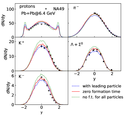
Figure 4: Same as Fig. 3, but the results from JAM + hydro simulations in which leading particles are also converted into fluid after their formation times (dashed lines), the results from the calculations without formation times but leading particles are not converted into fluid (solid lines), and the results from the calculations without formation times for all particles including leading particles.

In our default implementation, leading particles are not converted into fluid, and the other particles are converted into fluid after their formation times. To see the effects of our model assumptions, we have performed several calculations with different implementations. In Fig. 4, the results of the simulations in which the leading particles are also incorporated in the fluid after their formation times are shown. It is seen that baryon stopping power becomes less, and particle yields are also somewhat less than the default calculations. This may be because we have less initial hard collisions which are responsible to the particle productions and rapidity loss of leading hadrons. To see the effects of the formation time, we plot the results of calculations in which newly produced particles are converted into fluid with zero formation time in Fig. 4. The results show that there are no strong sensitivities of the particle productions to the formation times.

However, as depicted by the dotted lines in Fig. 4, when all particles are converted into fluid without formation times, we see the overprediction of strange particles and stronger proton stopping, since this implementation has similar effects as the one-fluid simulations. In any cases, particle production is not strongly affected by the details of implementations.

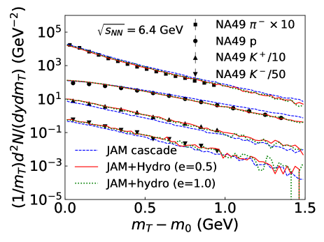
Figure 5: Transverse mass distributions of protons, negative pions, positive and negative kaons in central Pb + Pb collisions at $\sqrt{s_{{\scriptscriptstyle NN}}}=6.4$ GeV. The results from JAM cascade (dashed lines) and JAM + hydro calculations with $e_{\text{f}}=0.5$ (solid lines) and 1.0 GeV/fm³ (dotted lines) are compared with experimental data Alt:2007aa ; Alt:2006dk .

In Fig. 5, the transverse mass distributions of identified particles are depicted. The hybrid simulation exhibits similar slopes for the transverse mass distributions of pions and kaons to cascade simulations, and they are in good agreement with the data. It is also observed that the differences with respect to the parameter of the fluidization energy density are practically invisible. The harder proton slopes than the experimental data predicted by nonequilibrium transport approach in the JAM cascade model is improved by the hybrid model calculations.

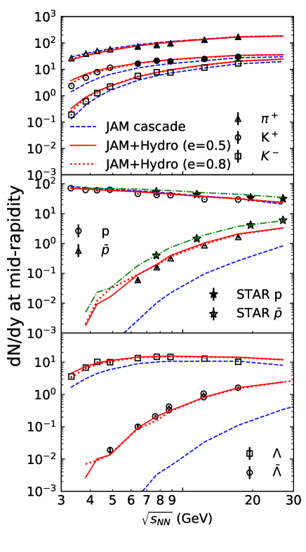
Figure 6: Beam energy dependence of particle multiplicities at midrapidity in central Au + Au and Pb + Pb collisions. The experimental data are taken from Ref. Ahle:1999uy ; NA49compilation ; Blume:2011sb ; Ahle:1998jc ; Klay:2001tf . JAM+hydro results for (anti-)protons with weak-decay contributions (dashed-dotted lines) are compared with the STAR data which contain the weak-decay feed-down contributions to (anti)-proton yield.

Figure 6 shows the beam-energy dependence of the particle yields $dN/dy$ at midrapidity $|y|<0.5$ for positively charged pions and kaons, negatively charged kaons, protons, antiprotons, $\Lambda$s, and anti-$\Lambda$s from the cascade and the hybrid simulations. JAM cascade model slightly overestimates pion yields at $\sqrt{s_{{\scriptscriptstyle NN}}}<10$ GeV, and underestimates strange particles. It is known that most of the standard microscopic transport models overestimate pion yields Weber:2002pk ; Wagner:2004ee ; Konchakovski:2014gda . Here the JAM+hydro hybrid approach improves this situation: hybrid calculations suppress pion yields and enhance strange particles, and good agreement with the data is obtained. It should be emphasized that the antibaryon productions such as antiprotons and anti-$\Lambda$s are also significantly improved, and good agreement with the data is obtained by the hybrid model. We have checked the dependence of the fluidization energy density $e_{\text{f}}$ on the multiplicities. The results from a larger value of $e_{\text{f}}=0.8$ GeV/fm³ relative to the value of $e_{\text{f}}=0.5$ GeV/fm³ yield less strange particles at lower beam energies, but its influence on the strange particle yields is very small at higher beam energies.

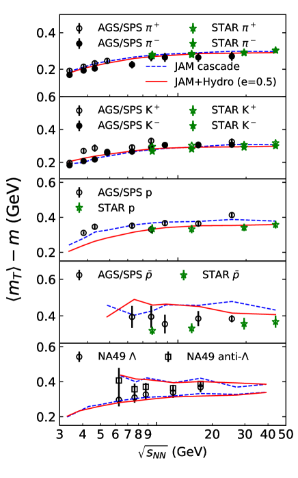
Figure 7: Beam-energy dependence of mean transverse mass for pions, kaons, protons, antiprotons, $\Lambda$s, and anti-$\Lambda$s at midrapidity in central Au + Au/Pb + Pb collisions. The experimental data are taken from Ref. Adamczyk:2017iwn ; Abelev:2009bw ; Alt:2008qm ; Alt:2006dk .

Figure 7 depicts the beam-energy dependence of the mean transverse mass for pions, kaons, protons, antiprotons, $\Lambda$s, and $\bar{\Lambda}$s compared with the experimental data Adamczyk:2017iwn ; Abelev:2009bw ; Alt:2008qm ; Alt:2006dk . We observe that the mean transverse mass in cascade is essentially unaffected by the hydrodynamics except protons, and models reproduce the experimental data of pions and kaons very well. The JAM cascade approach describes the proton slopes better at lower beam energies $\sqrt{s_{{\scriptscriptstyle NN}}}\leq 5$ GeV compared with the hybrid approach, while the hybrid approach describes proton slopes better at higher energies. We do not show the results with $e_{\text{f}}=1.0$ GeV/fm³, because the dependence of the mean transverse mass spectra on the fluidization energy densities is very small.

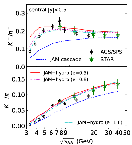
Figure 8: Beam-energy dependence of $K/\pi$ ratios at midrapidity in central Au + Au and Pb + Pb collisions. The experimental data are taken from Ref. Adamczyk:2017iwn ; Afanasiev:2002mx ; Alt:2007aa .

Let us turn now to the discussion of strange particle to pion ratios. Beam energy dependence of the $K/\pi$ ratios is shown in Fig. 8. Our hybrid approach significantly improves the description of the data over the predictions from JAM cascade. To see the dependence on the fluidization energy density $e_{\text{f}}$, we tested three different values of $e_{\text{f}}=0.5,0.8$, and 1.0 GeV/fm³. Larger values of $e_{\text{f}}$ improve the description of $K/\pi$ ratios at AGS energies, while it does not affect the higher beam energies much. This suggests that the value of $e_{\text{f}}=0.5$ GeV/fm³ may overestimate the thermal part of the system at lower beam energies. In the 3FD model, the strange particle productions at low beam energies are overestimated Ivanov:2013yla ; Batyuk:2016qmb . They introduced a beam energy dependent phenomenological strangeness suppression factor $\gamma_{s}$ at $\sqrt{s_{{\scriptscriptstyle NN}}}\leq 5$ GeV to suppress the yield of strange hadrons. It was found in the UrQMD hybrid approach that implementation of the core-corona separation of the system reduces the ratios involving strange particles Steinheimer:2011mp . The statistical models can reproduce the structure of the $K^{+}/\pi^{+}$ ratio by taking into account canonical suppression of the strangeness Andronic:2005yp ; Andronic:2008gu or introducing the strangeness suppression factor for the deviation from chemical equilibrium Becattini:2003wp ; Becattini:2005xt . In our approach, good agreement of the $K/\pi$ ratio with the data is achieved by the partial thermalization in both space and time. Note that in hybrid approaches, the nonthermal part of the system, which is described by the JAM transport model, is in general neither chemically nor kinetically equilibrated. Inclusion of the effects of thermal part is essential for a good description of the $K/\pi$ ratio within a dynamical model based on hydrodynamics.

We note that the PHSD transport model reproduces the $K/\pi$ ratio by the strange particle enhancement due to chiral symmetry restoration at high baryon densities without assuming any thermalization Cassing:2015owa . As a future work, incorporation of the dynamical treatment of a first-order chiral phase transition in a nonequilibrium real-time dynamics Paech:2003fe ; Herold:2013qda into our framework may improve significantly the description of collision dynamics and may show some signal of a QGP phase transition as well as the chiral symmetry restoration for some observables.

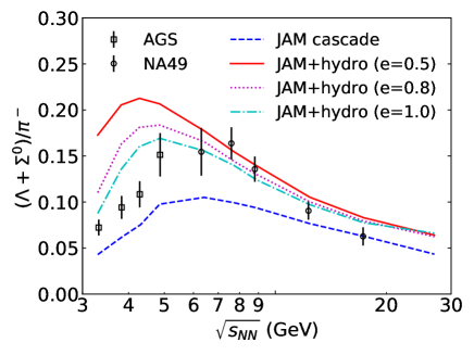
Figure 9: Beam energy dependence of $(\Lambda+\Sigma^{0})/\pi^{-}$ ratio at midrapidity in central Au + Au and Pb + Pb collisions. The experimental data are taken from Ref. Anticic:2003ux ; Aggarwal:2010ig .

Finally, the beam-energy dependence of $(\Lambda+\Sigma^{0})/\pi^{-}$ ratio is shown in Fig. 9 obtained by different values of fluidization energy densities. Good description of the data is obtained at high beam energies above $\sqrt{s_{{\scriptscriptstyle NN}}}=5$ GeV, but there is an overestimation at lower energies by the hybrid model, which may suggest that the conditions of the fluidization depend on beam energy or additional suppression of the strangeness due to nonchemical equilibration in the fluid part.

IV Conclusion

We have developed a dynamically integrated transport model for heavy-ion collisions at high baryon densities, in which nonequilibrium dynamics is solved by the hadronic transport model, and a dense part of the system is simultaneously described by hydrodynamical evolution. In this approach, dynamical coupling is implemented through the source terms of the fluid equations. For the fluidization of particles, we take into account core-corona separation, where only the high-density part of the system (core) follows the hydrodynamical evolution. We demonstrate that our integrated dynamical approach describes well the experimental data on the particle yields, transverse mass distributions, and particle ratios for a wide range of beam energies $3<\sqrt{s_{{\scriptscriptstyle NN}}}<30$ GeV for central Au + Au and Pb + Pb collisions. We found that partial thermalization of the system is very important to explain strange particle-to-pion ratios, $K^{\pm}/\pi^{\pm}$ and $(\Lambda+\Sigma^{0})/\pi^{-}$.

As future studies, we plan to perform systematic studies of the centrality dependence of various observables including multistrange particles and antibaryons. The EoS dependence on the particle productions as well as viscous effects in the hydrodynamical evolution should be investigated. In this work, we do not consider possible fluid-particle interactions; particles that go through dense region are likely to deposit their energies to the fluid or be absorbed by the fluid. These effects may become important for the quantitative description of some observables. It is also interesting to look at anisotropic flows such as directed and elliptic flows within our approach, which are expected to be very sensitive to the collision dynamics.

- (1) M. M. Aggarwal et al. [STAR Collaboration], arXiv:1007.2613 [nucl-ex].
- (2) L. Kumar, Mod. Phys. Lett. A 28, 1330033 (2013).
- (3) L. Adamczyk et al. [STAR Collaboration], Phys. Rev. C 96, no. 4, 044904 (2017).
- (4) L. Turko [NA61/SHINE Collaboration], Universe, 4, 52 (2018).
- (5) B. Friman, C. Hohne, J. Knoll, S. Leupold, J. Randrup, R. Rapp, and P. Senger, Lect. Notes Phys. 814, pp.1 (2011).
- (6) G. Odyniec, EPJ Web Conf. 95, 03027 (2015).
- (7) T. Ablyazimov et al. [CBM Collaboration], Eur. Phys. J. A 53, no. 3, 60 (2017).
- (8) V. Kekelidze, A. Kovalenko, R. Lednicky, V. Matveev, I. Meshkov, A. Sorin, and G. Trubnikov, Nucl. Phys. A 956, 846 (2016).
- (9) H. Sako et al., [J-PARC Heavy-Ion Collaboration], Nucl. Phys. A 931 1158 (2014); Nucl. Phys. A 956, 850 (2016).
- (10) G. Baym, T. Hatsuda, T. Kojo, P. D. Powell, Y. Song, and T. Takatsuka, Rept. Prog. Phys. 81, no. 5, 056902 (2018).
- (11) B. P. Abbott et al. [LIGO Scientific and Virgo Collaborations], Phys. Rev. Lett. 119, no. 16, 161101 (2017).
- (12) Y. Sekiguchi, K. Kiuchi, K. Kyutoku, and M. Shibata, Phys. Rev. Lett. 107, 051102 (2011).
- (13) M. Asakawa and K. Yazaki, Nucl. Phys. A 504, 668 (1989); D. H. Rischke, Prog. Part. Nucl. Phys. 52, 197(2004); M. A. Stephanov, Prog. Theor. Phys. Suppl. 153, 139(2004) [Int. J. Mod. Phys.A 20, 4387(2005)]; K. Fukushima and C. Sasaki, Prog. Part. Nucl. Phys. 72, 99(2013).
- (14) U. Heinz and R. Snellings, Ann. Rev. Nucl. Part. Sci. 63, 123 (2013).
- (15) C. Gale, S. Jeon, and B. Schenke, Int. J. Mod. Phys. A 28, 1340011 (2013).
- (16) P. Huovinen, Int. J. Mod. Phys. E 22, 1330029 (2013).
- (17) T. Hirano, P. Huovinen, K. Murase, and Y. Nara, Prog. Part. Nucl. Phys. 70, 108 (2013).
- (18) S. Jeon and U. Heinz, Int. J. Mod. Phys. E 24, no. 10, 1530010 (2015).
- (19) A. Jaiswal and V. Roy, Adv. High Energy Phys. 2016, 9623034 (2016).
- (20) P. Romatschke and U. Romatschke, arXiv:1712.05815 [nucl-th].
- (21) S. Pratt, E. Sangaline, P. Sorensen and H. Wang, Phys. Rev. Lett. 114, 202301 (2015).
- (22) J. E. Bernhard, J. S. Moreland, S. A. Bass, J. Liu and U. Heinz, Phys. Rev. C 94, no. 2, 024907 (2016).
- (23) J. Brachmann, A. Dumitru, J. A. Maruhn, H. Stoecker, W. Greiner, and D. H. Rischke, Nucl. Phys. A 619, 391 (1997).
- (24) Y. B. Ivanov, V. N. Russkikh, and V. D. Toneev, Phys. Rev. C 73, 044904 (2006).
- (25) Y. B. Ivanov, Phys. Rev. C 89, no. 2, 024903 (2014); Phys. Rev. C 87, no. 6, 064905 (2013); Phys. Rev. C 87, no. 6, 064904 (2013).
- (26) P. Batyuk et al., Phys. Rev. C 94, 044917 (2016).
- (27) Y. B. Ivanov and A. A. Soldatov, Phys. Rev. C 97, no. 2, 024908 (2018).
- (28) J. Steinheimer, M. Bleicher, H. Petersen, S. Schramm, H. Stocker, and D. Zschiesche, Phys. Rev. C 77, 034901 (2008).
- (29) H. Petersen, J. Steinheimer, G. Burau, M. Bleicher, and H. Stocker, Phys. Rev. C 78, 044901 (2008).
- (30) K. Werner, Phys. Rev. Lett. 98, 152301 (2007).
- (31) J. Steinheimer and M. Bleicher, Phys. Rev. C 84, 024905 (2011).
- (32) I. A. Karpenko, P. Huovinen, H. Petersen and M. Bleicher, Phys. Rev. C 91, no. 6, 064901 (2015).
- (33) J. Auvinen, J. E. Bernhard, S. A. Bass and I. Karpenko, Phys. Rev. C 97, no. 4, 044905 (2018).
- (34) M. Okai, K. Kawaguchi, Y. Tachibana, and T. Hirano, Phys. Rev. C 95, no. 5, 054914 (2017).
- (35) C. Shen and B. Schenke, Phys. Rev. C 97, no. 2, 024907 (2018).
- (36) M. Gazdzicki and M. I. Gorenstein, Acta Phys. Polon. B 30, 2705 (1999).
- (37) S. V. Afanasiev et al. [NA49 Collaboration], Phys. Rev. C 66, 054902 (2002).
- (38) C. Alt et al. [NA49 Collaboration], Phys. Rev. C 77, 024903 (2008).
- (39) A. Andronic, P. Braun-Munzinger, and J. Stachel, Nucl. Phys. A 772, 167 (2006).
- (40) A. Andronic, P. Braun-Munzinger, and J. Stachel, Phys. Lett. B 673, 142 (2009) Erratum: [Phys. Lett. B 678, 516 (2009)].
- (41) L. M. Satarov, M. N. Dmitriev, and I. N. Mishustin, Phys. Atom. Nucl. 72, 1390 (2009).
- (42) F. Becattini, M. Gazdzicki, A. Keranen, J. Manninen, and R. Stock, Phys. Rev. C 69, 024905 (2004).
- (43) F. Becattini, J. Manninen, and M. Gazdzicki, Phys. Rev. C 73, 044905 (2006).
- (44) W. Cassing, A. Palmese, P. Moreau, and E. L. Bratkovskaya, Phys. Rev. C 93, 014902 (2016); A. Palmese, W. Cassing, E. Seifert, T. Steinert, P. Moreau, and E. L. Bratkovskaya, Phys. Rev. C 94, no. 4, 044912 (2016).
- (45) Y. Nara, N. Otuka, A. Ohnishi, K. Niita, and S. Chiba, Phys. Rev. C 61, 024901 (2000).
- (46) H. Sorge, Phys. Rev. C 52, 3291 (1995).
- (47) S. A. Bass et al., Prog. Part. Nucl. Phys. 41, 255 (1998).
- (48) M. Bleicher et al., J. Phys. G 25, 1859 (1999).
- (49) M. Gyulassy and X. N. Wang, Comput. Phys. Commun. 83, 307 (1994).
- (50) T. Sjostrand, S. Mrenna, and P. Z. Skands, JHEP 0605 (2006), 026.
- (51) T. Hirano and Y. Nara, PTEP 2012, 01A203 (2012).
- (52) M. Isse, A. Ohnishi, N. Otuka, P. K. Sahu, and Y. Nara, Phys. Rev. C 72, 064908 (2005).
- (53) Y. Nara, H. Niemi, A. Ohnishi, and H. Stoecker, Phys. Rev. C 94, no. 3, 034906 (2016).
- (54) Y. Nara, H. Niemi, J. Steinheimer, and H. Stoecker, Phys. Lett. B 769, 543 (2017).
- (55) Y. Nara, H. Niemi, A. Ohnishi, J. Steinheimer, X. Luo, and H. Stoecker, Eur. Phys. J. A 54, no. 2, 18 (2018).
- (56) A. Bazavov et al. [HotQCD Collaboration], Phys. Rev. D 90, 094503 (2014).
- (57) D. Oliinychenko and H. Petersen, Phys. Rev. C 93, no. 3, 034905 (2016).
- (58) V. Schneider, U. Katscher, D. H. Rischke, B. Waldhauser, J. A. Maruhn, and C. D. Munz, J. Comput. Phys. 105, 92 (1993).
- (59) D. H. Rischke, S. Bernard, J.A.Maruhn, Nucl. Phys. A595 (1995) 346.
- (60) I. Karpenko, P. Huovinen, and M. Bleicher, Comput. Phys. Commun. 185, 3016 (2014).
- (61) B. Van Leer, J. Comput. Phys. 32, 101 (1979).
- (62) K. Okamoto and C. Nonaka, Eur. Phys. J. C 77, no. 6, 383 (2017).
- (63) A. Bazavov et al., Phys. Rev. D 95, no. 5, 054504 (2017).
- (64) J. Sollfrank, P. Huovinen, M. Kataja, P. V. Ruuskanen, M. Prakash, and R. Venugopalan, Phys. Rev. C 55, 392 (1997); P. F. Kolb, J. Sollfrank, and U. W. Heinz, Phys. Lett. B 459, 667 (1999); P. F. Kolb, J. Sollfrank, and U. W. Heinz, Phys. Rev. C 62, 054909 (2000).
- (65) F. Cooper and G. Frye, Phys. Rev. D 10, 186 (1974).
- (66) P. Huovinen and H. Petersen, Eur. Phys. J. A 48, 171 (2012).
- (67) S. Pratt, Phys. Rev. C 89, no. 2, 024910 (2014).
- (68) C. Alt et al. [NA49 Collaboration], Phys. Rev. C 78, 034918 (2008) doi:10.1103/PhysRevC.78.034918 [arXiv:0804.3770 [nucl-ex]].
- (69) C. Blume [Na49 Collaboration], J. Phys. G 34, S951 (2007).
- (70) C. Alt et al. [NA49 Collaboration], Phys. Rev. C 73, 044910 (2006).
- (71) L. Ahle et al. [E866 and E917 Collaborations], Phys. Lett. B 476, 1 (2000).
- (72) C. Blume, M. Gazdzicki, B. Lungwitz, M. Mitrovski, P. Seyboth, and H. Stroebele, NA49 Compilation, https://edms.cern.ch/document/1075059.
- (73) C. Blume and C. Markert, Prog. Part. Nucl. Phys. 66, 834 (2011).
- (74) L. Ahle et al. [E-802 Collaboration], Phys. Rev. C 57, no. 2, R466 (1998).
- (75) J. L. Klay et al. [E895 Collaboration], Phys. Rev. Lett. 88, 102301 (2002).
- (76) H. Weber, E. L. Bratkovskaya, W. Cassing, and H. Stoecker, Phys. Rev. C 67, 014904 (2003).
- (77) M. Wagner, A. B. Larionov, and U. Mosel, Phys. Rev. C 71, 034910 (2005).
- (78) V. P. Konchakovski, W. Cassing, Y. B. Ivanov, and V. D. Toneev, Phys. Rev. C 90, no. 1, 014903 (2014).
- (79) B. I. Abelev et al. [STAR Collaboration], Phys. Rev. C 81, 024911 (2010).
- (80) C. Alt et al. [NA49 Collaboration], Phys. Rev. C 78, 034918 (2008).
- (81) T. Anticic et al. [NA49 Collaboration], Phys. Rev. Lett. 93, 022302 (2004).
- (82) M. M. Aggarwal et al. [STAR Collaboration], Phys. Rev. C 83, 024901 (2011).
- (83) K. Paech, H. Stoecker and A. Dumitru, Phys. Rev. C 68, 044907 (2003).
- (84) C. Herold, M. Nahrgang, I. Mishustin and M. Bleicher, Nucl. Phys. A 925, 14 (2014).