Bilingual Sentiment Embeddings:
Joint Projection of Sentiment Across Languages

Abstract

Sentiment analysis in low-resource languages suffers from a lack of annotated corpora to estimate high-performing models. Machine translation and bilingual word embeddings provide some relief through cross-lingual sentiment approaches. However, they either require large amounts of parallel data or do not sufficiently capture sentiment information. We introduce Bilingual Sentiment Embeddings (Blse), which jointly represent sentiment information in a source and target language. This model only requires a small bilingual lexicon, a source-language corpus annotated for sentiment, and monolingual word embeddings for each language. We perform experiments on three language combinations (Spanish, Catalan, Basque) for sentence-level cross-lingual sentiment classification and find that our model significantly outperforms state-of-the-art methods on four out of six experimental setups, as well as capturing complementary information to machine translation. Our analysis of the resulting embedding space provides evidence that it represents sentiment information in the resource-poor target language without any annotated data in that language.

1 Introduction

Cross-lingual approaches to sentiment analysis are motivated by the lack of training data in the vast majority of languages. Even languages spoken by several million people, such as Catalan, often have few resources available to perform sentiment analysis in specific domains. We therefore aim to harness the knowledge previously collected in resource-rich languages.

Previous approaches for cross-lingual sentiment analysis typically exploit machine translation based methods or multilingual models. Machine translation (Mt) can provide a way to transfer sentiment information from a resource-rich to resource-poor languages Mihalcea et al. (2007); Balahur and Turchi (2014). However, Mt-based methods require large parallel corpora to train the translation system, which are often not available for under-resourced languages.

Examples of multilingual methods that have been applied to cross-lingual sentiment analysis include domain adaptation methods Prettenhofer and Stein (2011), delexicalization Almeida et al. (2015), and bilingual word embeddings Mikolov et al. (2013); Hermann and Blunsom (2014); Artetxe et al. (2016). These approaches however do not incorporate enough sentiment information to perform well cross-lingually, as we will show later.

We propose a novel approach to incorporate sentiment information in a model, which does not have these disadvantages. Bilingual Sentiment Embeddings (Blse) are embeddings that are jointly optimized to represent both (a) semantic information in the source and target languages, which are bound to each other through a small bilingual dictionary, and (b) sentiment information, which is annotated on the source language only. We only need three resources: (i) a comparably small bilingual lexicon, (ii) an annotated sentiment corpus in the resource-rich language, and (iii) monolingual word embeddings for the two involved languages.

We show that our model outperforms previous state-of-the-art models in nearly all experimental settings across six benchmarks. In addition, we offer an in-depth analysis and demonstrate that our model is aware of sentiment. Finally, we provide a qualitative analysis of the joint bilingual sentiment space. Our implementation is publicly available at https://github.com/jbarnesspain/blse.

2 Related Work

Machine Translation: Early work in cross-lingual sentiment analysis found that machine translation (Mt) had reached a point of maturity that enabled the transfer of sentiment across languages. Researchers translated sentiment lexicons Mihalcea et al. (2007); Meng et al. (2012) or annotated corpora and used word alignments to project sentiment annotation and create target-language annotated corpora Banea et al. (2008); Duh et al. (2011); Demirtas and Pechenizkiy (2013); Balahur and Turchi (2014).

Several approaches included a multi-view representation of the data Banea et al. (2010); Xiao and Guo (2012) or co-training Wan (2009); Demirtas and Pechenizkiy (2013) to improve over a naive implementation of machine translation, where only the translated data is used. There are also approaches which only require parallel data Meng et al. (2012); Zhou et al. (2016); Rasooli et al. (2017), instead of machine translation.

All of these approaches, however, require large amounts of parallel data or an existing high quality translation tool, which are not always available. A notable exception is the approach proposed by Chen et al. (2016), an adversarial deep averaging network, which trains a joint feature extractor for two languages. They minimize the difference between these features across languages by learning to fool a language discriminator, which requires no parallel data. It does, however, require large amounts of unlabeled data.

Bilingual Embedding Methods:

Recently proposed bilingual embedding methods Hermann and Blunsom (2014); Chandar et al. (2014); Gouws et al. (2015) offer a natural way to bridge the language gap. These particular approaches to bilingual embeddings, however, require large parallel corpora in order to build the bilingual space, which are not available for all language combinations.

An approach to create bilingual embeddings that has a less prohibitive data requirement is to create monolingual vector spaces and then learn a projection from one to the other. Mikolov et al. (2013) find that vector spaces in different languages have similar arrangements. Therefore, they propose a linear projection which consists of learning a rotation and scaling matrix. Artetxe et al. (2016, 2017) improve upon this approach by requiring the projection to be orthogonal, thereby preserving the monolingual quality of the original word vectors.

Given source embeddings $S$, target embeddings $T$, and a bilingual lexicon $L$, Artetxe et al. (2016) learn a projection matrix $W$ by minimizing the square of Euclidean distances

$$\operatorname*{arg\,min}_{W}\sum_{i}||S^{\prime}W-T^{\prime}||_{F}^{2}\,,$$ (1)

where $S^{\prime}\in S$ and $T^{\prime}\in T$ are the word embedding matrices for the tokens in the bilingual lexicon $L$. This is solved using the Moore-Penrose pseudoinverse $S^{\prime+}=(S^{\prime T}S^{\prime})^{-1}S^{\prime T}$ as $W=S^{\prime+}T^{\prime}$, which can be computed using SVD. We refer to this approach as Artetxe.

Gouws and Søgaard (2015) propose a method to create a pseudo-bilingual corpus with a small task-specific bilingual lexicon, which can then be used to train bilingual embeddings (Barista). This approach requires a monolingual corpus in both the source and target languages and a set of translation pairs. The source and target corpora are concatenated and then every word is randomly kept or replaced by its translation with a probability of 0.5. Any kind of word embedding algorithm can be trained with this pseudo-bilingual corpus to create bilingual word embeddings.

These last techniques have the advantage of requiring relatively little parallel training data while taking advantage of larger amounts of monolingual data. However, they are not optimized for sentiment.
Sentiment Embeddings: Maas et al. (2011) first explored the idea of incorporating sentiment information into semantic word vectors. They proposed a topic modeling approach similar to latent Dirichlet allocation in order to collect the semantic information in their word vectors. To incorporate the sentiment information, they included a second objective whereby they maximize the probability of the sentiment label for each word in a labeled document.

Tang et al. (2014) exploit distantly annotated tweets to create Twitter sentiment embeddings. To incorporate distributional information about tokens, they use a hinge loss and maximize the likelihood of a true $n$-gram over a corrupted $n$-gram. They include a second objective where they classify the polarity of the tweet given the true $n$-gram. While these techniques have proven useful, they are not easily transferred to a cross-lingual setting.

Zhou et al. (2015) create bilingual sentiment embeddings by translating all source data to the target language and vice versa. This requires the existence of a machine translation system, which is a prohibitive assumption for many under-resourced languages, especially if it must be open and freely accessible. This motivates approaches which can use smaller amounts of parallel data to achieve similar results.

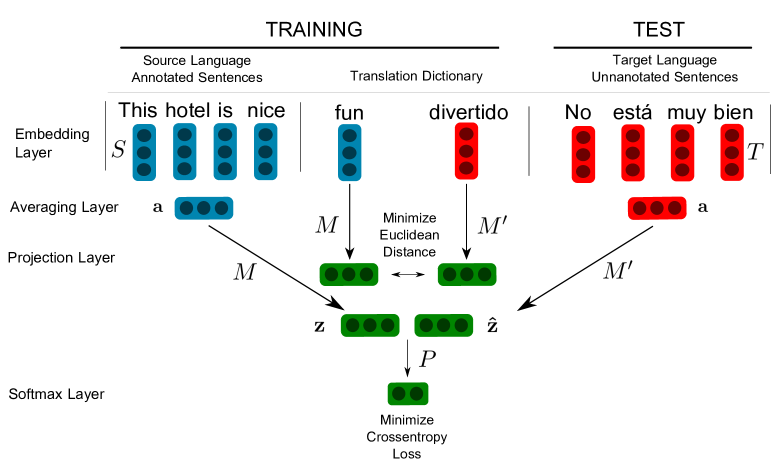
Figure 1: Bilingual Sentiment Embedding Model (Blse)

3 Model

In order to project not only semantic similarity and relatedness but also sentiment information to our target language, we propose a new model, namely Bilingual Sentiment Embeddings (BLSE), which jointly learns to predict sentiment and to minimize the distance between translation pairs in vector space. We detail the projection objective in Section 3.1, the sentiment objective in Section 3.2, and the full objective in Section 3.3. A sketch of the model is depicted in Figure 1.

3.1 Cross-lingual Projection

We assume that we have two precomputed vector spaces $S=\mathbb{R}^{v\times d}$ and $T=\mathbb{R}^{v^{\prime}\times d^{\prime}}$ for our source and target languages, where $v$ ($v^{\prime}$) is the length of the source vocabulary (target vocabulary) and $d$ ($d^{\prime}$) is the dimensionality of the embeddings. We also assume that we have a bilingual lexicon $L$ of length $n$ which consists of word-to-word translation pairs $L$ = $\{(s_{1},t_{1}),(s_{2},t_{2}),\ldots,(s_{n},t_{n})\}$ which map from source to target.

In order to create a mapping from both original vector spaces $S$ and $T$ to shared sentiment-informed bilingual spaces $\mathbf{z}$ and $\mathbf{\hat{z}}$, we employ two linear projection matrices, $M$ and $M^{\prime}$. During training, for each translation pair in $L$, we first look up their associated vectors, project them through their associated projection matrix and finally minimize the mean squared error of the two projected vectors. This is very similar to the approach taken by Mikolov et al. (2013), but includes an additional target projection matrix.

The intuition for including this second matrix is that a single projection matrix does not support the transfer of sentiment information from the source language to the target language. Without $M^{\prime}$, any signal coming from the sentiment classifier (see Section 3.2) would have no affect on the target embedding space $T$, and optimizing $M$ to predict sentiment and projection would only be detrimental to classification of the target language. We analyze this further in Section 6.3. Note that in this configuration, we do not need to update the original vector spaces, which would be problematic with such small training data.

The projection quality is ensured by minimizing the mean squared error

$$\textrm{MSE}=\dfrac{1}{n}\sum_{i=1}^{n}(\mathbf{z_{i}}-\mathbf{\hat{z}_{i}})^{2}\,,$$ (2)

where $\mathbf{z_{i}}=S_{s_{i}}\cdot M$ is the dot product of the embedding for source word $s_{i}$ and the source projection matrix and $\mathbf{\hat{z}_{i}}=T_{t_{i}}\cdot M^{\prime}$ is the same for the target word $t_{i}$.

3.2 Sentiment Classification

We add a second training objective to optimize the projected source vectors to predict the sentiment of source phrases. This inevitably changes the projection characteristics of the matrix $M$, and consequently $M^{\prime}$ and encourages $M^{\prime}$ to learn to predict sentiment without any training examples in the target language.

To train $M$ to predict sentiment, we require a source-language corpus $C_{\textrm{source}}=\{(x_{1},y_{1}),(x_{2},y_{2}),\ldots,(x_{i},y_{i})\}$ where each sentence $x_{i}$ is associated with a label $y_{i}$.

For classification, we use a two-layer feed-forward averaging network, loosely following Iyyer et al. (2015). For a sentence $x_{i}$ we take the word embeddings from the source embedding $S$ and average them to $\mathbf{a}_{i}\in\mathbb{R}^{d}$. We then project this vector to the joint bilingual space $\mathbf{z}_{i}=\mathbf{a}_{i}\cdot M$. Finally, we pass $\mathbf{z}_{i}$ through a softmax layer $P$ to get our prediction $\hat{y}_{i}=\textrm{softmax}(\mathbf{z}_{i}\cdot P)$.

To train our model to predict sentiment, we minimize the cross-entropy error of our predictions

$$H=-\sum_{i=1}^{n}y_{i}\log\hat{y_{i}}-(1-y_{i})\log(1-\hat{y_{i}})\,.$$ (3)

3.3 Joint Learning

In order to jointly train both the projection component and the sentiment component, we combine the two loss functions to optimize the parameter matrices $M$, $M^{\prime}$, and $P$ by

$$J=\kern-14.22636pt\sum_{(x,y)\in C_{\textrm{source}}}\kern-2.84526pt\sum_{(s,t)\in L}\kern-2.84526pt\alpha H(x,y)+(1-\alpha)\cdot\textrm{MSE}(s,t)\,,$$ (4)

where $\alpha$ is a hyperparameter that weights sentiment loss vs. projection loss.

		EN	ES	CA	EU
Binary	$+$	1258	1216	718	956
	$-$	473	256	467	173
	Total	1731	1472	1185	1129
4-class	$++$	379	370	256	384
	$+$	879	846	462	572
	$-$	399	218	409	153
	$--$	74	38	58	20
	Total	1731	1472	1185	1129

Table 1: Statistics for the OpeNER English (EN) and Spanish (ES) as well as the MultiBooked Catalan (CA) and Basque (EU) datasets.

3.4 Target-language Classification

For inference, we classify sentences from a target-language corpus $C_{\textrm{target}}$. As in the training procedure, for each sentence, we take the word embeddings from the target embeddings $T$ and average them to $\mathbf{a}_{i}\in\mathbb{R}^{d}$. We then project this vector to the joint bilingual space $\mathbf{\hat{z}}_{i}=\mathbf{a}_{i}\cdot M^{\prime}$. Finally, we pass $\mathbf{\hat{z}}_{i}$ through a softmax layer $P$ to get our prediction $\hat{y}_{i}=\textrm{softmax}(\mathbf{\hat{z}}_{i}\cdot P)$.

4 Datasets and Resources

4.1 OpeNER and MultiBooked

To evaluate our proposed model, we conduct experiments using four benchmark datasets and three bilingual combinations. We use the OpeNER English and Spanish datasets Agerri et al. (2013) and the MultiBooked Catalan and Basque datasets Barnes et al. (2018). All datasets contain hotel reviews which are annotated for aspect-level sentiment analysis. The labels include Strong Negative ($--$), Negative ($-$), Positive ($+$), and Strong Positive ($++$). We map the aspect-level annotations to sentence level by taking the most common label and remove instances of mixed polarity. We also create a binary setup by combining the strong and weak classes. This gives us a total of six experiments. The details of the sentence-level datasets are summarized in Table 1.

	Spanish	Catalan	Basque
Sentences	23 M	9.6 M	0.7 M
Tokens	610 M	183 M	25 M
Embeddings	0.83 M	0.4 M	0.14 M

Table 2: Statistics for the Wikipedia corpora and monolingual vector spaces.

For each of the experiments, we take 70 percent of the data for training, 20 percent for testing and the remaining 10 percent are used as development data for tuning.

4.2 Monolingual Word Embeddings

For Blse, Artetxe, and Mt, we require monolingual vector spaces for each of our languages. For English, we use the publicly available GoogleNews vectors. For Spanish, Catalan, and Basque, we train skip-gram embeddings using the Word2Vec toolkit with 300 dimensions, subsampling of $10^{-4}$, window of 5, negative sampling of 15 based on a 2016 Wikipedia corpus (sentence-split, tokenized with IXA pipes Agerri et al. (2014) and lowercased). The statistics of the Wikipedia corpora are given in Table 2.

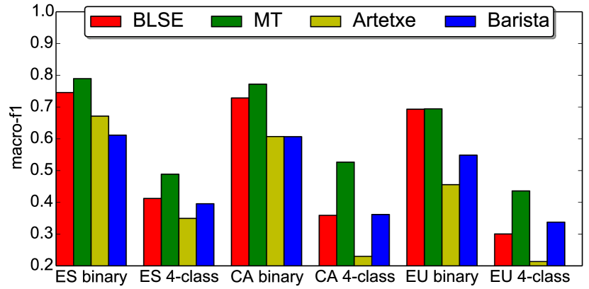
Figure 2: Binary and four class macro $\text{F}_{1}$ on Spanish (ES), Catalan (CA), and Basque (EU).

4.3 Bilingual Lexicon

For Blse, Artetxe, and Barista, we also require a bilingual lexicon. We use the sentiment lexicon from Hu and Liu (2004) (to which we refer in the following as Bing Liu) and its translation into each target language. We translate the lexicon using Google Translate and exclude multi-word expressions. This leaves a dictionary of 5700 translations in Spanish, 5271 in Catalan, and 4577 in Basque. We set aside ten percent of the translation pairs as a development set in order to check that the distances between translation pairs not seen during training are also minimized during training.

5 Experiments

5.1 Setting

We compare Blse (Sections 3.1–3.3) to Artetxe (Section 2) and Barista (Section 2) as baselines, which have similar data requirements and to machine translation (Mt) and monolingual (Mono) upper bounds which request more resources. For all models (Mono, Mt, Artetxe, Barista), we take the average of the word embeddings in the source-language training examples and train a linear SVM. We report this instead of using the same feed-forward network as in Blse as it is the stronger upper bound. We choose the parameter $c$ on the target language development set and evaluate on the target language test set.

			Binary			4-class
			ES	CA	EU	ES	CA	EU
Upper Bounds	Mono	P	75.0	79.0	74.0	55.2	50.0	48.3
		R	72.3	79.6	67.4	42.8	50.9	46.5
		$\text{F}_{1}$	73.5	79.2	69.8	45.5	49.9	47.1
	Mt	P	82.3	78.0	75.6	51.8	58.9	43.6
		R	76.6	76.8	66.5	48.5	50.5	45.2
		$\text{F}_{1}$	79.0	77.2	69.4	48.8	52.7	43.6
	BLSE	P	72.1	**72.8	**67.5	**60.0	38.1	*42.5
		R	**80.1	**73.0	**72.7	*43.4	38.1	37.4
		$\text{F}_{1}$	**74.6	**72.9	**69.3	*41.2	35.9	30.0
Baselines	Artetxe	P	75.0	60.1	42.2	40.1	21.6	30.0
		R	64.3	61.2	49.5	36.9	29.8	35.7
		$\text{F}_{1}$	67.1	60.7	45.6	34.9	23.0	21.3
	Barista	P	64.7	65.3	55.5	44.1	36.4	34.1
		R	59.8	61.2	54.5	37.9	38.5	34.3
		$\text{F}_{1}$	61.2	60.1	54.8	39.5	36.2	33.8
Ensemble	Artetxe	P	65.3	63.1	70.4	43.5	46.5	50.1
		R	61.3	63.3	64.3	44.1	48.7	50.7
		$\text{F}_{1}$	62.6	63.2	66.4	43.8	47.6	49.9
	Barista	P	60.1	63.4	50.7	48.3	52.8	50.8
		R	55.5	62.3	50.4	46.6	53.7	49.8
		$\text{F}_{1}$	56.0	62.5	49.8	47.1	53.0	47.8
	BLSE	P	79.5	84.7	80.9	49.5	54.1	50.3
		R	78.7	85.5	69.9	51.2	53.9	51.4
		$\text{F}_{1}$	80.3	85.0	73.5	50.3	53.9	50.5

Table 3: Precision (P), Recall (R), and macro $\text{F}_{1}$ of four models trained on English and tested on Spanish (ES), Catalan (CA), and Basque (EU). The bold numbers show the best results for each metric per column and the highlighted numbers show where Blse is better than the other projection methods, Artetxe and Barista (** p $<$ 0.01, * p $<$ 0.05).

Upper Bound Mono. We set an empirical upper bound by training and testing a linear SVM on the target language data. As mentioned in Section 5.1, we train the model on the averaged embeddings from target language training data, tuning the $c$ parameter on the development data. We test on the target language test data.

Upper Bound Mt. To test the effectiveness of machine translation, we translate all of the sentiment corpora from the target language to English using the Google Translate API. Note that this approach is not considered a baseline, as we assume not to have access to high-quality machine translation for low-resource languages of interest.

Baseline Artetxe. We compare with the approach proposed by Artetxe et al. (2016) which has shown promise on other tasks, such as word similarity. In order to learn the projection matrix $W$, we need translation pairs. We use the same word-to-word bilingual lexicon mentioned in Section 3.1. We then map the source vector space $S$ to the bilingual space $\hat{S}=SW$ and use these embeddings.

Baseline Barista. We also compare with the approach proposed by Gouws and Søgaard (2015). The bilingual lexicon used to create the pseudo-bilingual corpus is the same word-to-word bilingual lexicon mentioned in Section 3.1. We follow the authors’ setup to create the pseudo-bilingual corpus. We create bilingual embeddings by training skip-gram embeddings using the Word2Vec toolkit on the pseudo-bilingual corpus using the same parameters from Section 4.2.

Our method: BLSE. We implement our model Blse in Pytorch Paszke et al. (2016) and initialize the word embeddings with the pretrained word embeddings $S$ and $T$ mentioned in Section 4.2. We use the word-to-word bilingual lexicon from Section 4.3, tune the hyperparameters $\alpha$, training epochs, and batch size on the target development set and use the best hyperparameters achieved on the development set for testing. ADAM Kingma and Ba (2014) is used in order to minimize the average loss of the training batches.

Ensembles We create an ensemble of Mt and each projection method (Blse, Artetxe, Barista) by training a random forest classifier on the predictions from Mt and each of these approaches. This allows us to evaluate to what extent each projection model adds complementary information to the machine translation approach.

Model		voc	mod	neg	know	other	total
Mt	bi	49	26	19	14	5	113
	4	147	94	19	21	12	293
Artetxe	bi	80	44	27	14	7	172
	4	182	141	19	24	19	385
Barista	bi	89	41	27	20	7	184
	4	191	109	24	31	15	370
Blse	bi	67	45	21	15	8	156
	4	146	125	29	22	19	341

Table 4: Error analysis for different phenomena. See text for explanation of error classes.

5.2 Results

In Figure 2, we report the results of all four methods. Our method outperforms the other projection methods (the baselines Artetxe and Barista) on four of the six experiments substantially. It performs only slightly worse than the more resource-costly upper bounds (Mt and Mono). This is especially noticeable for the binary classification task, where Blse performs nearly as well as machine translation and significantly better than the other methods. We perform approximate randomization tests Yeh (2000) with 10,000 runs and highlight the results that are statistically significant (**p $<$ 0.01, *p $<$ 0.05) in Table 3.

In more detail, we see that Mt generally performs better than the projection methods (79–69 $\text{F}_{1}$ on binary, 52–44 on 4-class). Blse (75–69 on binary, 41–30 on 4-class) has the best performance of the projection methods and is comparable with Mt on the binary setup, with no significant difference on binary Basque. Artetxe (67–46 on binary, 35–21 on 4-class) and Barista (61–55 on binary, 40–34 on 4-class) are significantly worse than Blse on all experiments except Catalan and Basque 4-class. On the binary experiment, Artetxe outperforms Barista on Spanish (67.1 vs. 61.2) and Catalan (60.7 vs. 60.1) but suffers more than the other methods on the four-class experiments, with a maximum $\text{F}_{1}$ of 34.9. Barista is relatively stable across languages.

Ensemble performs the best, which shows that Blse adds complementary information to Mt. Finally, we note that all systems perform successively worse on Catalan and Basque. This is presumably due to the quality of the word embeddings, as well as the increased morphological complexity of Basque.

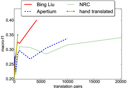
Figure 3: Macro $\text{F}_{1}$ for translation pairs in the Spanish 4-class setup.

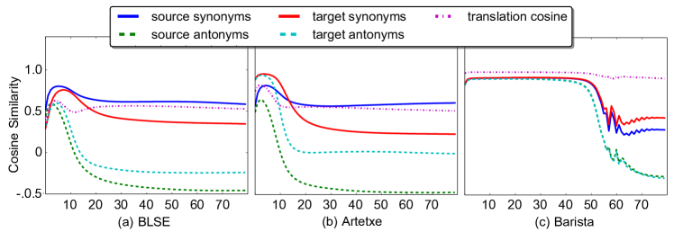
Figure 4: Average cosine similarity between a subsample of translation pairs of same polarity (“sentiment synonyms”) and of opposing polarity (“sentiment antonyms”) in both target and source languages in each model. The x-axis shows training epochs. We see that Blse is able to learn that sentiment synonyms should be close to one another in vector space and sentiment antonyms should not.

6 Model and Error Analysis

We analyze three aspects of our model in further detail: (i) where most mistakes originate, (ii) the effect of the bilingual lexicon, and (iii) the effect and necessity of the target-language projection matrix $M^{\prime}$.

6.1 Phenomena

In order to analyze where each model struggles, we categorize the mistakes and annotate all of the test phrases with one of the following error classes: vocabulary (voc), adverbial modifiers (mod), negation (neg), external knowledge (know) or other. Table 4 shows the results.

Vocabulary: The most common way to express sentiment in hotel reviews is through the use of polar adjectives (as in “the room was great) or the mention of certain nouns that are desirable (“it had a pool”). Although this phenomenon has the largest total number of mistakes (an average of 71 per model on binary and 167 on 4-class), it is mainly due to its prevalence. Mt performed the best on the test examples which according to the annotation require a correct understanding of the vocabulary (81 $\text{F}_{1}$ on binary /54 $\text{F}_{1}$ on 4-class), with Blse (79/48) slightly worse. Artetxe (70/35) and Barista (67/41) perform significantly worse. This suggests that Blse is better Artetxe and Barista at transferring sentiment of the most important sentiment bearing words.

Negation: Negation is a well-studied phenomenon in sentiment analysis Pang et al. (2002); Wiegand et al. (2010); Zhu et al. (2014); Reitan et al. (2015). Therefore, we are interested in how these four models perform on phrases that include the negation of a key element, for example “In general, this hotel isn’t bad”. We would like our models to recognize that the combination of two negative elements “isn’t” and “bad” lead to a Positive label.

Given the simple classification strategy, all models perform relatively well on phrases with negation (all reach nearly 60 $\text{F}_{1}$ in the binary setting). However, while Blse performs the best on negation in the binary setting (82.9 $\text{F}_{1}$), it has more problems with negation in the 4-class setting (36.9 $\text{F}_{1}$).

Adverbial Modifiers: Phrases that are modified by an adverb, e. g., the food was incredibly good, are important for the four-class setup, as they often differentiate between the base and Strong labels. In the binary case, all models reach more than 55 $\text{F}_{1}$. In the 4-class setup, Blse only achieves 27.2 $\text{F}_{1}$ compared to 46.6 or 31.3 of Mt and Barista, respectively. Therefore, presumably, our model does currently not capture the semantics of the target adverbs well. This is likely due to the fact that it assigns too much sentiment to functional words (see Figure 6).

External Knowledge Required: These errors are difficult for any of the models to get correct. Many of these include numbers which imply positive or negative sentiment (350 meters from the beach is Positive while 3 kilometers from the beach is Negative). Blse performs the best (63.5 $\text{F}_{1}$) while Mt performs comparably well (62.5). Barista performs the worst (43.6).

Binary vs. 4-class: All of the models suffer when moving from the binary to 4-class setting; an average of 26.8 in macro $\text{F}_{1}$ for Mt, 31.4 for Artetxe, 22.2 for Barista, and for 36.6 Blse. The two vector projection methods (Artetxe and Blse) suffer the most, suggesting that they are currently more apt for the binary setting.

6.2 Effect of Bilingual Lexicon

We analyze how the number of translation pairs affects our model. We train on the 4-class Spanish setup using the best hyper-parameters from the previous experiment.

Research into projection techniques for bilingual word embeddings Mikolov et al. (2013); Lazaridou et al. (2015); Artetxe et al. (2016) often uses a lexicon of the most frequent 8–10 thousand words in English and their translations as training data. We test this approach by taking the 10,000 word-to-word translations from the Apertium English-to-Spanish dictionary. We also use the Google Translate API to translate the NRC hashtag sentiment lexicon Mohammad et al. (2013) and keep the 22,984 word-to-word translations. We perform the same experiment as above and vary the amount of training data from 0, 100, 300, 600, 1000, 3000, 6000, 10,000 up to 20,000 training pairs. Finally, we compile a small hand translated dictionary of 200 pairs, which we then expand using target language morphological information, finally giving us 657 translation pairs. The macro $\text{F}_{1}$ score for the Bing Liu dictionary climbs constantly with the increasing translation pairs. Both the Apertium and NRC dictionaries perform worse than the translated lexicon by Bing Liu, while the expanded hand translated dictionary is competitive, as shown in Figure 3.

While for some tasks, e. g., bilingual lexicon induction, using the most frequent words as translation pairs is an effective approach, for sentiment analysis, this does not seem to help. Using a translated sentiment lexicon, even if it is small, gives better results.

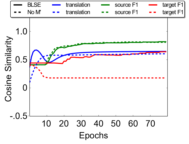
Figure 5: Blse model (solid lines) compared to a variant without target language projection matrix $M^{\prime}$ (dashed lines). “Translation” lines show the average cosine similarity between translation pairs. The remaining lines show $\text{F}_{1}$ scores for the source and target language with both varints of Blse. The modified model cannot learn to predict sentiment in the target language (red lines). This illustrates the need for the second projection matrix $M^{\prime}$.

6.3 Analysis of $M^{\prime}$

The main motivation for using two projection matrices $M$ and $M^{\prime}$ is to allow the original embeddings to remain stable, while the projection matrices have the flexibility to align translations and separate these into distinct sentiment subspaces. To justify this design decision empirically, we perform an experiment to evaluate the actual need for the target language projection matrix $M^{\prime}$: We create a simplified version of our model without $M^{\prime}$, using $M$ to project from the source to target and then $P$ to classify sentiment.

The results of this model are shown in Figure 5. The modified model does learn to predict in the source language, but not in the target language. This confirms that $M^{\prime}$ is necessary to transfer sentiment in our model.

7 Qualitative Analyses of Joint Bilingual Sentiment Space

In order to understand how well our model transfers sentiment information to the target language, we perform two qualitative analyses. First, we collect two sets of 100 positive sentiment words and one set of 100 negative sentiment words. An effective cross-lingual sentiment classifier using embeddings should learn that two positive words should be closer in the shared bilingual space than a positive word and a negative word. We test if Blse is able to do this by training our model and after every epoch observing the mean cosine similarity between the sentiment synonyms and sentiment antonyms after projecting to the joint space.

We compare Blse with Artetxe and Barista by replacing the Linear SVM classifiers with the same multi-layer classifier used in Blse and observing the distances in the hidden layer. Figure 4 shows this similarity in both source and target language, along with the mean cosine similarity between a held-out set of translation pairs and the macro $\text{F}_{1}$ scores on the development set for both source and target languages for Blse, Barista, and Artetxe. From this plot, it is clear that Blse is able to learn that sentiment synonyms should be close to one another in vector space and antonyms should have a negative cosine similarity. While the other models also learn this to some degree, jointly optimizing both sentiment and projection gives better results.

Secondly, we would like to know how well the projected vectors compare to the original space. Our hypothesis is that some relatedness and similarity information is lost during projection. Therefore, we visualize six categories of words in t-SNE Van der Maaten and Hinton (2008): positive sentiment words, negative sentiment words, functional words, verbs, animals, and transport.

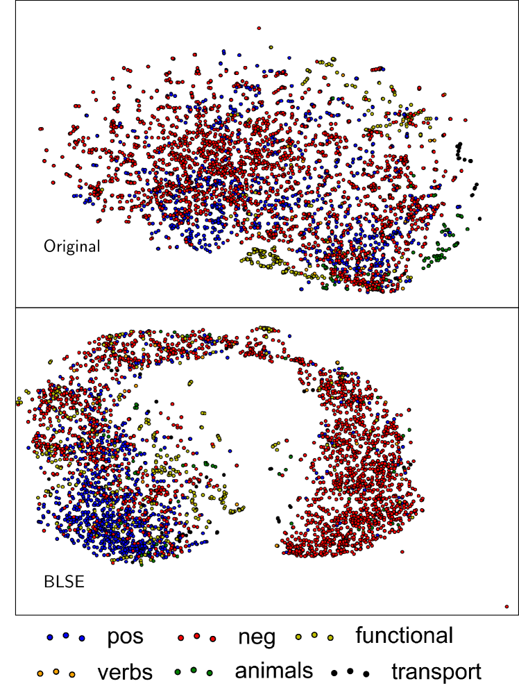
Figure 6: t-SNE-based visualization of the Spanish vector space before and after projection with Blse. There is a clear separation of positive and negative words after projection, despite the fact that we have used no labeled data in Spanish.

The t-SNE plots in Figure 6 show that the positive and negative sentiment words are rather clearly separated after projection in Blse. This indicates that we are able to incorporate sentiment information into our target language without any labeled data in the target language. However, the downside of this is that functional words and transportation words are highly correlated with positive sentiment.

8 Conclusion

We have presented a new model, Blse, which is able to leverage sentiment information from a resource-rich language to perform sentiment analysis on a resource-poor target language. This model requires less parallel data than Mt and performs better than other state-of-the-art methods with similar data requirements, an average of 14 percentage points in $\text{F}_{1}$ on binary and 4 pp on 4-class cross-lingual sentiment analysis. We have also performed a phenomena-driven error analysis which showed that Blse is better than Artetxe and Barista at transferring sentiment, but assigns too much sentiment to functional words. In the future, we will extend our model so that it can project multi-word phrases, as well as single words, which could help with negations and modifiers.

References

- Agerri et al. (2014) Rodrigo Agerri, Josu Bermudez, and German Rigau. 2014. Ixa pipeline: Efficient and ready to use multilingual nlp tools. In Proceedings of the Ninth International Conference on Language Resources and Evaluation (LREC’14). pages 3823–3828.
- Agerri et al. (2013) Rodrigo Agerri, Montse Cuadros, Sean Gaines, and German Rigau. 2013. OpeNER: Open polarity enhanced named entity recognition. Sociedad Española para el Procesamiento del Lenguaje Natural 51(Septiembre):215–218.
- Almeida et al. (2015) Mariana S. C. Almeida, Claudia Pinto, Helena Figueira, Pedro Mendes, and André F. T. Martins. 2015. Aligning opinions: Cross-lingual opinion mining with dependencies. In Proceedings of the 53rd Annual Meeting of the Association for Computational Linguistics and the 7th International Joint Conference on Natural Language Processing (Volume 1: Long Papers). pages 408–418.
- Artetxe et al. (2016) Mikel Artetxe, Gorka Labaka, and Eneko Agirre. 2016. Learning principled bilingual mappings of word embeddings while preserving monolingual invariance. In Proceedings of the 2016 Conference on Empirical Methods in Natural Language Processing. pages 2289–2294.
- Artetxe et al. (2017) Mikel Artetxe, Gorka Labaka, and Eneko Agirre. 2017. Learning bilingual word embeddings with (almost) no bilingual data. In Proceedings of the 55th Annual Meeting of the Association for Computational Linguistics (Volume 1: Long Papers). pages 451–462.
- Balahur and Turchi (2014) Alexandra Balahur and Marco Turchi. 2014. Comparative experiments using supervised learning and machine translation for multilingual sentiment analysis. Computer Speech & Language 28(1):56–75.
- Banea et al. (2010) Carmen Banea, Rada Mihalcea, and Janyce Wiebe. 2010. Multilingual subjectivity: Are more languages better? In Proceedings of the 23rd International Conference on Computational Linguistics (Coling 2010). pages 28–36.
- Banea et al. (2008) Carmen Banea, Rada Mihalcea, Janyce Wiebe, and Samer Hassan. 2008. Multilingual subjectivity analysis using machine translation. In Proceedings of the 2008 Conference on Empirical Methods in Natural Language Processing. pages 127–135.
- Barnes et al. (2018) Jeremy Barnes, Patrik Lambert, and Toni Badia. 2018. Multibooked: A corpus of basque and catalan hotel reviews annotated for aspect-level sentiment classification. In Proceedings of 11th Language Resources and Evaluation Conference (LREC’18).
- Chandar et al. (2014) Sarath Chandar, Stanislas Lauly, Hugo Larochelle, Mitesh Khapra, Balaraman Ravindran, Vikas C Raykar, and Amrita Saha. 2014. An autoencoder approach to learning bilingual word representations. In Z. Ghahramani, M. Welling, C. Cortes, N. D. Lawrence, and K. Q. Weinberger, editors, Advances in Neural Information Processing Systems 27, Curran Associates, Inc., pages 1853–1861.
- Chen et al. (2016) Xilun Chen, Ben Athiwaratkun, Yu Sun, Kilian Q. Weinberger, and Claire Cardie. 2016. Adversarial deep averaging networks for cross-lingual sentiment classification. CoRR abs/1606.01614. http://arxiv.org/abs/1606.01614.
- Demirtas and Pechenizkiy (2013) Erkin Demirtas and Mykola Pechenizkiy. 2013. Cross-lingual polarity detection with machine translation. Proceedings of the International Workshop on Issues of Sentiment Discovery and Opinion Mining - WISDOM ’13 pages 9:1–9:8.
- Duh et al. (2011) Kevin Duh, Akinori Fujino, and Masaaki Nagata. 2011. Is machine translation ripe for cross-lingual sentiment classification? Proceedings of the 49th Annual Meeting of the Association for Computational Linguistics: Human Language Technologies: short papers 2:429–433.
- Gouws et al. (2015) Stephan Gouws, Yoshua Bengio, and Greg Corrado. 2015. BilBOWA: Fast bilingual distributed representations without word alignments. Proceedings of The 32nd International Conference on Machine Learning pages 748–756.
- Gouws and Søgaard (2015) Stephan Gouws and Anders Søgaard. 2015. Simple task-specific bilingual word embeddings. In Proceedings of the 2015 Conference of the North American Chapter of the Association for Computational Linguistics: Human Language Technologies. pages 1386–1390.
- Hermann and Blunsom (2014) Karl Moritz Hermann and Phil Blunsom. 2014. Multilingual models for compositional distributed semantics. In Proceedings of the 52nd Annual Meeting of the Association for Computational Linguistics (Volume 1: Long Papers). Association for Computational Linguistics, Baltimore, Maryland, pages 58–68.
- Hu and Liu (2004) Minqing Hu and Bing Liu. 2004. Mining opinion features in customer reviews. In Proceedings of the 10th ACM SIGKDD International Conference on Knowledge Discovery and Data Mining (KDD 2004). pages 168–177.
- Iyyer et al. (2015) Mohit Iyyer, Varun Manjunatha, Jordan Boyd-Graber, and Hal Daume III. 2015. Deep unordered composition rivals syntactic methods for text classification. In Proceedings of the 53rd Annual Meeting of the Association for Computational Linguistics and the 7th International Joint Conference on Natural Language Processing (Volume 1: Long Papers). Beijing, China, pages 1681–1691.
- Kingma and Ba (2014) Diederik Kingma and Jimmy Ba. 2014. Adam: A method for stochastic optimization. Proceedings of the 3rd International Conference on Learning Representations (ICLR) .
- Lazaridou et al. (2015) Angeliki Lazaridou, Georgiana Dinu, and Marco Baroni. 2015. Hubness and pollution: delving into cross-space mapping for zero-shot learning. Proceedings of the 53rd Annual Meeting of the Association for Computational Linguistics and the 7th International Joint Conference on Natural Language Processing pages 270–280.
- Maas et al. (2011) Andrew L. Maas, Raymond E. Daly, Peter T. Pham, Dan Huang, Andrew Y. Ng, and Christopher Potts. 2011. Learning word vectors for sentiment analysis. In Proceedings of the 49th Annual Meeting of the Association for Computational Linguistics: Human Language Technologies. pages 142–150.
- Meng et al. (2012) Xinfan Meng, Furu Wei, Xiaohua Liu, Ming Zhou, Ge Xu, and Houfeng Wang. 2012. Cross-lingual mixture model for sentiment classification. In Proceedings of the 50th Annual Meeting of the Association for Computational Linguistics (Volume 1: Long Papers). Association for Computational Linguistics, Jeju Island, Korea, pages 572–581. http://www.aclweb.org/anthology/P12-1060.
- Mihalcea et al. (2007) Rada Mihalcea, Carmen Banea, and Janyce Wiebe. 2007. Learning multilingual subjective language via cross-lingual projections. In Proceedings of the 45th Annual Meeting of the Association of Computational Linguistics. pages 976–983.
- Mikolov et al. (2013) Tomas Mikolov, Quoc V. Le, and Ilya Sutskever. 2013. Exploiting similarities among languages for machine translation. CoRR abs/1309.4168. http://arxiv.org/abs/1309.4168.
- Mohammad et al. (2013) Saif M. Mohammad, Svetlana Kiritchenko, and Xiaodan Zhu. 2013. Nrc-canada: Building the state-of-the-art in sentiment analysis of tweets. In Proceedings of the seventh international workshop on Semantic Evaluation Exercises (SemEval-2013).
- Pang et al. (2002) Bo Pang, Lillian Lee, and Shivakumar Vaithyanathan. 2002. Thumbs up? sentiment classification using machine learning techniques. In Proceedings of the ACL-02 Conference on Empirical methods in natural language processing-Volume 10. Association for Computational Linguistics, pages 79–86.
- Paszke et al. (2016) Adam Paszke, Sam Gross, Soumith Chintala, and Gregory Chanan. 2016. Pytorch deeplearning framework. http://pytorch.org. Accessed: 2017-08-10.
- Prettenhofer and Stein (2011) Peter Prettenhofer and Benno Stein. 2011. Cross-lingual adaptation using structural correspondence learning. ACM Transactions on Intelligent Systems and Technology 3(1):1–22.
- Rasooli et al. (2017) Mohammad Sadegh Rasooli, Noura Farra, Axinia Radeva, Tao Yu, and Kathleen McKeown. 2017. Cross-lingual sentiment transfer with limited resources. Machine Translation .
- Reitan et al. (2015) Johan Reitan, Jørgen Faret, Björn Gambäck, and Lars Bungum. 2015. Negation scope detection for twitter sentiment analysis. In Proceedings of the 6th Workshop on Computational Approaches to Subjectivity, Sentiment and Social Media Analysis. pages 99–108.
- Tang et al. (2014) Duyu Tang, Furu Wei, Nan Yang, Ming Zhou, Ting Liu, and Bing Qin. 2014. Learning sentiment-specific word embedding for twitter sentiment classification. In Proceedings of the 52nd Annual Meeting of the Association for Computational Linguistics (Volume 1: Long Papers). pages 1555–1565.
- Van der Maaten and Hinton (2008) Laurens Van der Maaten and Geoffrey Hinton. 2008. Visualizing data using t-sne. Journal of Machine Learning Research 9:2579–2605.
- Wan (2009) Xiaojun Wan. 2009. Co-training for cross-lingual sentiment classification. In Proceedings of the Joint Conference of the 47th Annual Meeting of the ACL and the 4th International Joint Conference on Natural Language Processing of the AFNLP. pages 235–243.
- Wiegand et al. (2010) Michael Wiegand, Alexandra Balahur, Benjamin Roth, Dietrich Klakow, and Andrés Montoyo. 2010. A survey on the role of negation in sentiment analysis. In Proceedings of the Workshop on Negation and Speculation in Natural Language Processing. pages 60–68.
- Xiao and Guo (2012) Min Xiao and Yuhong Guo. 2012. Multi-view adaboost for multilingual subjectivity analysis. In Proceedings of COLING 2012. pages 2851–2866.
- Yeh (2000) Alexander Yeh. 2000. More accurate tests for the statistical significance of result differences. In Proceedings of the 18th Conference on Computational linguistics (COLING). pages 947–953.
- Zhou et al. (2016) Guangyou Zhou, Zhiyuan Zhu, Tingting He, and Xiaohua Tony Hu. 2016. Cross-lingual sentiment classification with stacked autoencoders. Knowledge and Information Systems 47(1):27–44.
- Zhou et al. (2015) HuiWei Zhou, Long Chen, Fulin Shi, and Degen Huang. 2015. Learning bilingual sentiment word embeddings for cross-language sentiment classification. In Proceedings of the 53rd Annual Meeting of the Association for Computational Linguistics and the 7th International Joint Conference on Natural Language Processing (Volume 1: Long Papers). pages 430–440.
- Zhu et al. (2014) Xiaodan Zhu, Hongyu Guo, Saif Mohammad, and Svetlana Kiritchenko. 2014. An empirical study on the effect of negation words on sentiment. In Proceedings of the 52nd Annual Meeting of the Association for Computational Linguistics (Volume 1: Long Papers). pages 304–313.