Propriety of the reference posterior distribution in Gaussian Process modeling

Abstract

In a seminal article, Berger, De Oliveira and Sansó (2001) compare several objective prior distributions for the parameters of Gaussian Process models with isotropic correlation kernel. The reference prior distribution stands out among them insofar as it always leads to a proper posterior. They prove this result for rough correlation kernels - Spherical, Exponential with power $\rho<2$, Matérn with smoothness $\nu<1$. This paper provides a proof for smooth correlation kernels - Exponential with power $\rho=2$, Matérn with smoothness $\nu\geqslant 1$, Rational Quadratic - along with tail rates of the reference prior for these kernels.

arXiv:1805.08992

1 Introduction

Gaussian processes are often used to emulate unknown functions from some space $\mathbb{R}^{r}$ ($r\geqslant 1$) to $\mathbb{R}$ (Rasmussen and Williams, 2006). Interpreted in Bayesian terms, this analysis sets the distribution of a Gaussian process as the prior distribution of the unknown function. The posterior is still Gaussian, but conditioned on the values of the function observed at specific points of $\mathbb{R}^{r}$. In order to show the performance of such models, upper bounds for posterior rates have been obtained by van der Vaart and van Zanten (2008) and lower bounds by Castillo (2008).

The Gaussian prior distribution is usually parametric, with the parameters typically set to the maximum likelihood estimator. Another approach is hierarchical Bayesian modeling, where a prior on the parameters of the prior Gaussian process distribution is defined. This approach is extensively discussed in Chapter 6 of Banerjee, Carlin and Gelfand (2004).

Given prior knowledge about the parameters of the Gaussian prior is often lacking, there is value in objective elicitation of their prior distribution.

However, De Oliveira, Kedem and Short (1997) and Stein (1999) noted that commonly used noninformative priors sometimes failed to yield proper posteriors. Berger, De Oliveira and Sansó (2001) were the first to thoroughly investigate the issue. Among several prior distributions – truncated priors, vague priors, Jeffreys-rule and independence Jeffreys prior – they showed that the reference prior (Bernardo, 2005) is the most satisfying choice for a default prior distribution. This is due to the fact that, for all isotropic correlation kernels studied by Berger, De Oliveira and Sansó (2001), the reference prior yields a proper posterior distribution. In the following, whenever we mention a “prior”, it is the prior on the parameters of the Gaussian process distribution, not the Gaussian process distribution itself.

Posterior propriety is necessary to Bayesian procedures aiming to quantify parameter uncertainty: it would make no sense to express parameter uncertainty through a posterior distribution that does not integrate to a finite mass. Moreover, in spatial models, one may want to take parameter uncertainty into account when performing prediction. Prediction can be averaged over a proper posterior distribution on parameters, not an improper one.

In this article, we complete the proof by Berger, De Oliveira and Sansó (2001) that the reference posterior is proper. Because of the difficulty involved in obtaining a satisfying default prior distribution which consistently yields a proper posterior, it is important to ascertain that the reference prior actually does. Indeed, a vast literature builds upon this result.

Provided some additional conditions on the design set and the mean function are verified, Paulo (2005) states that the reference posterior is also proper with anisotropic product correlation kernels that have specific properties. As Paulo (2005) notes, these properties are also necessary to make the proof from Berger, De Oliveira and Sansó (2001) work.

He then warns the reader that the Squared Exponential kernel (Power Exponential with power $\rho=2$) does not satisfy one of them.

Ren, Sun and He (2012) investigate the propriety of reference posteriors for isotropic correlation kernels with an additional noise term (nugget effect). They show that the reference prior is not the same for different parameter orders, but that all reference priors lead to a proper posterior. However, the correlation kernel must have the same properties as those required by Berger, De Oliveira and Sansó (2001).

Kazianka and Pilz (2012) consider the same setting and focus on the reference prior with a particular parameter order. They provide an application to the analysis of zinc concentrations in the French river Meuse.

Ren, Sun and Sahu (2013) return to the setting explored by Paulo (2005) – anisotropic product correlation kernels – but relax his conditions on the mean function.

Gu, Wang and Berger (2018) go further still and also relax his conditions on the design set. Moreover, they establish reference posterior propriety with anisotropic product covariance kernels and an additional noise term (nugget effect). Their work thus generalizes and combines results from Paulo (2005) and Ren, Sun and Sahu (2013) on one side, Ren, Sun and He (2012) and Kazianka and Pilz (2012) on the other.

However, all these papers prove reference posterior propriety under similar assumptions as those made by Berger, De Oliveira and Sansó (2001). They rely on properties that only rough correlation kernels possess.

The main result of this work is Theorem 4.4, which ensures that the reference prior leads to a proper posterior distribution for a large class of smooth isotropic kernels. Secondary results include bounds on the reference prior density and on the function obtained after integrating several parameters out of the likelihood.

The paper is organized as follows. Section 2 describes the Gaussian Process models considered by Berger, De Oliveira and Sansó (2001). Section 3 shows that the proof of the propriety of the reference posterior provided by Berger, De Oliveira and Sansó (2001) only applies to Gaussian Process models with rough correlation kernels – Spherical, Exponential with power $\rho<2$, Matérn with smoothness $\nu<1$. Section 4 provides bounds on reference prior and integrated likelihood which are then used to prove that the reference posterior is also proper for models with smoother correlation kernels, including Exponential kernels with power $\rho=2$, Matérn kernels with smoothness $\nu\geqslant 1$ and Rational Quadratic kernels. While Section 4 provides bounds applying to all cases, tighter bounds applying to specific cases only are obtained in Appendix B.

2 Setting

Berger, De Oliveira and Sansó (2001) consider Gaussian Process models (also known as Universal Kriging models) with isotropic kernels. This article is set in their framework and borrows most of its notations from them. Define $\|\cdot\|$ as the usual Euclidean norm if applied to a vector and as the Frobenius norm if applied to a matrix. We denote integer intervals by $[\![\cdot,\cdot]\!]$: $[\![1,4]\!]$ for instance is the set $\{1,2,3,4\}$.

In Universal Kriging, an unknown function from a domain $\mathcal{D}\subset\mathbb{R}^{r}$ ($r\in\mathbb{Z}_{+}$) to $\mathbb{R}$ is assumed to be a realization of a Gaussian process $Y$. The mean function $f$ of the Gaussian process is assumed to belong to some known vector space $\mathcal{F}_{p}$ of dimension $p\in\mathbb{N}$. If $p$ is non-zero, once a basis $(f_{j})_{j\in[\![1,p]\!]}$ of $\mathcal{F}_{p}$ has been set, $f$ can be parametrized by $\boldsymbol{\beta}=(\beta_{1},...,\beta_{p})^{\top}\in\mathbb{R}^{p}$ such that $f=\sum_{j=1}^{p}\beta_{j}f_{j}$.

$Y-f$ is assumed to be a stationary Gaussian process based on an isotropic correlation kernel. An isotropic correlation kernel is a function $K:[0,+\infty)\rightarrow[-1,1]$ such that for any positive integer $n$ and any collection of $n$ distinct points $(\boldsymbol{x}^{(i)})_{i\in[\![1,n]\!]}$ within $\mathcal{D}$, the symmetric $n\times n$ matrix $\boldsymbol{\Sigma}$ with $(i,i^{\prime})$-th element $K(\|\boldsymbol{x}^{(i)}-\boldsymbol{x}^{(i^{\prime})}\|)$ is a positive definite correlation matrix. Necessarily, $K(0)=1$.

The covariance function of the Gaussian process $Y$ is $\sigma^{2}K_{\theta}$, where $K_{\theta}$ is the correlation kernel parametrized by $\theta\in(0,+\infty)$ and defined by $K_{\theta}(\cdot)=K(\cdot/\theta)$, making $\sigma^{2}\in(0,+\infty)$ the variance of $Y(\boldsymbol{x})$ for every $\boldsymbol{x}\in\mathcal{D}$.

Fix $n\in\mathbb{Z}_{+}$ and fix a collection of $n$ distinct points $(\boldsymbol{x}^{(i)})_{i\in[\![1,n]\!]}$.

Let this collection be the design set, i.e. the set of points where $Y$ is observed. $\left(Y(\boldsymbol{x}^{(1)}),...,Y(\boldsymbol{x}^{(n)})\right)^{\top}$ is a Gaussian vector. $\left(f(\boldsymbol{x}^{(1)}),...,f(\boldsymbol{x}^{(n)})\right)^{\top}$ is its mean vector and $\sigma^{2}\boldsymbol{\Sigma}_{\theta}$ its covariance matrix, with $\boldsymbol{\Sigma}_{\theta}$ being the $n\times n$ matrix with $(i,i^{\prime})$-th element $K_{\theta}(\|\boldsymbol{x}^{(i)}-\boldsymbol{x}^{(i^{\prime})}\|)$. Table 1 provides the definition of several correlation kernels.

Kernel	$K_{\theta}(t)$ (with $t\in(0,+\infty)$)	parameter range
Spherical	$\left(1-\frac{3}{2}\left(\frac{t}{\theta}\right)+\frac{1}{2}\left(\frac{t}{\theta}\right)^{3}\right)\boldsymbol{1}_{\{t\leqslant\theta\}}$	$\emptyset$
Power Exponential	$\exp\left\{-\left(\frac{t}{\theta}\right)^{\rho}\right\}$	$\rho\in(0,2]$
Rational Quadratic	$\left(1+\left(\frac{t}{\theta}\right)^{2}\right)^{-\nu}$	$\nu\in(0,+\infty)$
Matérn	$\Gamma(\nu)^{-1}2^{1-\nu}\left(2\sqrt{\nu}\frac{t}{\theta}\right)^{\nu}\mathcal{K}_{\nu}\left(2\sqrt{\nu}\frac{t}{\theta}\right)$	$\nu\in(0,+\infty)$

Table 1: Formulas for several correlation kernel families. The Spherical kernel can only be used if the design space is of dimension 1, 2 or 3, because it is not positive definite for greater dimensions (Stein, 1999). $\mathcal{K}_{\nu}$ is the modified Bessel function of second kind with parameter $\nu$ (Abramowitz and Stegun, 1964, section 9.6). This parametrization of the Matérn family is recommended by Handcock and Wallis (1994). To recover the one used by Berger, De Oliveira and Sansó (2001), simply replace $2\sqrt{\nu}t$ by $t$.

If $p$ is non-zero, let $\boldsymbol{H}$ denote the $n\times p$ matrix with $(i,j)$-th element $f_{j}(\boldsymbol{x}^{(i)})$. Then $\left(f(\boldsymbol{x}^{(1)}),...,f(\boldsymbol{x}^{(n)})\right)^{\top}=\boldsymbol{H}\boldsymbol{\beta}$. If $p=0$, then we adopt the convention that any term involving $\boldsymbol{H}$ can be ignored. Let us denote the observed value of the random vector $\left(Y(\boldsymbol{x}^{(1)}),...,Y(\boldsymbol{x}^{(n)})\right)^{\top}$ by $\boldsymbol{y}=(y_{1},...,y_{n})^{\top}$. The likelihood function of the parameter triplet $(\boldsymbol{\beta},\sigma^{2},\theta)^{\top}$ has the following expression:

$$L(\boldsymbol{y}\;|\;\boldsymbol{\beta},\sigma^{2},\boldsymbol{\theta})=\left(\frac{1}{2\pi\sigma^{2}}\right)^{\frac{n}{2}}|\boldsymbol{\Sigma}_{\theta}|^{-\frac{1}{2}}\exp\left\{-\frac{1}{2\sigma^{2}}(\boldsymbol{y}-\boldsymbol{H}\boldsymbol{\beta})^{\top}\boldsymbol{\Sigma}_{\theta}^{-1}(\boldsymbol{y}-\boldsymbol{H}\boldsymbol{\beta})\right\}.$$ (2.1)

In order for the model to be identifiable, assume that $p<n$ and that $\boldsymbol{H}$ has rank $p$.

Let us recall the general definition of the reference prior and how it is derived in this setting.

For smooth one-dimensional parametric families, the reference prior coincides with the Jeffreys-rule prior (Clarke and Barron, 1994). For smooth finite-dimensional parametric families, the reference prior algorithm requires the user to define groups of dimensions of the parameter and rank them. The reference prior is then defined iteratively (Bernardo, 2005):

1. Compute the Jeffreys-rule prior on the lowest-ranking group of dimensions conditionally on all others.

2. Average the likelihood function over this prior.

3. Compute the Jeffreys-rule prior (based on the integrated likelihood function) on the second-lowest-ranking group of dimensions conditionally on all higher-ranking dimensions.

4. Average the integrated likelihood function over this second prior.

5. Continue the process until the Jeffreys-rule prior on the highest-ranking group of dimensions has been computed.

6. The reference prior is defined as the product of all successively computed priors.

Berger, De Oliveira and Sansó (2001) treat $\boldsymbol{\beta}$ as the lowest-ranking (possibly multidimensional) parameter and view $(\sigma^{2},\theta)$ as a group of 2 equal-ranking parameters when they apply the reference prior algorithm. We denote this ordering by $\boldsymbol{\beta}\prec(\sigma^{2},\theta)$. This choice is not arbitrary: if $\sigma^{2}$ and $\theta$ were known, then the covariance matrix $\sigma^{2}\boldsymbol{\Sigma}_{\theta}$ would be known. Since the model is Gaussian, we would then know which linear transformation to apply to the observations to make them mutually independent. In the case of Simple Kriging, $\boldsymbol{\beta}$ is not used and their reference prior is simply the Jeffreys-rule prior. Note that $\theta$ is one-dimensional because all correlation kernels considered by Berger, De Oliveira and Sansó (2001) - which are also those covered in the present article - are isotropic.

Ren, Sun and He (2012) show that if we split the parameters further, with $\boldsymbol{\beta}$ remaining the lowest-ranking parameter, $\sigma^{2}$ being of middle rank and $\theta$ being the highest-ranking parameter, the reference prior algorithm yields the same reference prior. In other words, the reference prior for the ordering $\boldsymbol{\beta}\prec\sigma^{2}\prec\theta$ is the same as the reference prior for the ordering $\boldsymbol{\beta}\prec(\sigma^{2},\theta)$. It is this prior we consider in the present article.

To express it conveniently, denote $\boldsymbol{Q}_{\theta}:=\boldsymbol{I}_{n}-\boldsymbol{H}\left(\boldsymbol{H}^{\top}\boldsymbol{\Sigma}_{\theta}^{-1}\boldsymbol{H}\right)^{-1}\boldsymbol{H}^{\top}\boldsymbol{\Sigma}_{\theta}^{-1}$.

If $p=0$, $\boldsymbol{Q}_{\theta}:=\boldsymbol{I}_{n}$. Also fix $\boldsymbol{W}$, an $n\times(n-p)$ matrix such that $\boldsymbol{W}^{\top}\boldsymbol{W}=\boldsymbol{I}_{n-p}$ and $\boldsymbol{H}^{\top}\boldsymbol{W}$ is the $p\times(n-p)$ null matrix. The columns of $\boldsymbol{W}$ form an orthonormal basis of the orthogonal complement of the subspace of $\mathbb{R}^{n}$ spanned by the columns of $\boldsymbol{H}$. If $p=0$, fix $\boldsymbol{W}$ as an orthogonal matrix, for example $\boldsymbol{I}_{n}$.

If $p>0$, the matrix $\boldsymbol{W}$ can for instance be constructed by computing a Singular Value Decomposition (SVD) of $\boldsymbol{H}$. Let us write this decomposition $\boldsymbol{H}=\boldsymbol{U}\boldsymbol{S}\boldsymbol{V}^{\top}$. $\boldsymbol{U}$ and $\boldsymbol{V}$ are orthogonal matrices of size $n\times n$ and $p\times p$ respectively, and $\boldsymbol{S}$ is an $n\times p$ matrix whose only non-null entries are on the main diagonal. Therefore the last $n-p$ rows of $\boldsymbol{S}$ are filled with zeros. The matrix $\boldsymbol{W}$ can then be defined as the $n\times(n-p)$ matrix formed by the last $n-p$ columns of $\boldsymbol{U}$.

The next two propositions give formulas for the reference prior density and for the integrated likelihood. The latter is obtained by integrating the likelihood against the reference prior on $\boldsymbol{\beta}$ conditionally on $\sigma^{2}$ and $\theta$ and against the reference prior on $\sigma^{2}$ conditionally on $\theta$.

Proposition 2.1.

The reference prior with ordering $\boldsymbol{\beta}\prec(\sigma^{2},\theta)$ or $\boldsymbol{\beta}\prec\sigma^{2}\prec\theta$ is $\pi(\boldsymbol{\beta},\sigma^{2},\theta)\propto\left(\sigma^{2}\right)^{-1}\pi(\theta)$, where

$$\pi(\theta)\propto\sqrt{\operatorname{Tr}\left[\left\{\left(\frac{d}{d\theta}\boldsymbol{\Sigma}_{\theta}\right)\boldsymbol{\Sigma}_{\theta}^{-1}\boldsymbol{Q}_{\theta}\right\}^{2}\right]-\frac{1}{n-p}\left[\operatorname{Tr}\left\{\left(\frac{d}{d\theta}\boldsymbol{\Sigma}_{\theta}\right)\boldsymbol{\Sigma}_{\theta}^{-1}\boldsymbol{Q}_{\theta}\right\}\right]^{2}}.$$ (2.2)

Denoting $\boldsymbol{W}^{\top}\boldsymbol{\Sigma}_{\theta}\boldsymbol{W}$ by $\boldsymbol{\Sigma}_{\theta}^{\boldsymbol{W}}$, $\pi(\theta)$ can also be written as:

$$\pi(\theta)\propto\sqrt{\operatorname{Tr}\left[\left\{\left(\frac{d}{d\theta}\boldsymbol{\Sigma}_{\theta}^{\boldsymbol{W}}\right)\left(\boldsymbol{\Sigma}_{\theta}^{\boldsymbol{W}}\right)^{-1}\right\}^{2}\right]-\frac{1}{n-p}\left[\operatorname{Tr}\left\{\left(\frac{d}{d\theta}\boldsymbol{\Sigma}_{\theta}^{\boldsymbol{W}}\right)\left(\boldsymbol{\Sigma}_{\theta}^{\boldsymbol{W}}\right)^{-1}\right\}\right]^{2}}.$$ (2.3)

The fact that (2.2) is an expression of the reference prior fitting the ordering $\boldsymbol{\beta}\prec(\sigma^{2},\theta)$ was first shown in Berger, De Oliveira and Sansó (2001). Ren, Sun and He (2012) then showed that the reference prior fitting the ordering $\boldsymbol{\beta}\prec\sigma^{2}\prec\theta$ is the same. The proof that (2.3) is an expression of the same reference prior can be found in Appendix A.1.

Proposition 2.1 shows that $\pi(\theta)$ is the only untractable factor in the expression of the reference prior $\pi(\boldsymbol{\beta},\sigma^{2},\theta)$. The parameters $\boldsymbol{\beta}$ and $\sigma^{2}$ can be marginalized out of $L(\boldsymbol{y}|\boldsymbol{\beta},\sigma^{2},\theta)$.

Proposition 2.2.

If $p\geqslant 1$, after marginalizing $\boldsymbol{\beta}$ and $\sigma^{2}$ out, we have

$$L_{\boldsymbol{y}}(\theta) :=\iint L_{\boldsymbol{y}}(\boldsymbol{\beta},\sigma^{2},\theta)/\sigma^{2}d\boldsymbol{\beta}d\sigma^{2}$$

$$=\left(\frac{2\pi^{\frac{n-p}{2}}}{\Gamma\left(\frac{n-p}{2}\right)}\right)^{-1}\left|\boldsymbol{\Sigma}_{\theta}^{-1}\right|^{\frac{1}{2}}|\left|\boldsymbol{H}^{\top}\boldsymbol{\Sigma}_{\theta}^{-1}\boldsymbol{H}\right|^{-\frac{1}{2}}\left(\boldsymbol{y}^{\top}\boldsymbol{\Sigma}_{\theta}^{-1}\boldsymbol{Q}_{\theta}\boldsymbol{y}\right)^{-\frac{n-p}{2}}.$$ (2.4)

Alternatively, the integrated likelihood with $p\geqslant 1$ can also be written

$$L_{\boldsymbol{y}}(\theta)=\left(\frac{2\pi^{\frac{n-p}{2}}}{\Gamma\left(\frac{n-p}{2}\right)}\right)^{-1}\left|\boldsymbol{H}^{\top}\boldsymbol{H}\right|^{-\frac{1}{2}}\left|\boldsymbol{W}^{\top}\boldsymbol{\Sigma}_{\theta}\boldsymbol{W}\right|^{-\frac{1}{2}}\left(\boldsymbol{y}^{\top}\boldsymbol{W}\left(\boldsymbol{W}^{\top}\boldsymbol{\Sigma}_{\theta}\boldsymbol{W}\right)^{-1}\boldsymbol{W}^{\top}\boldsymbol{y}\right)^{-\frac{n-p}{2}}.$$ (2.5)

If $p=0$, the integrated likelihood is simply

$$L_{\boldsymbol{y}}(\theta)=\int L_{\boldsymbol{y}}(\sigma^{2},\theta)/\sigma^{2}d\sigma^{2}=\left(\frac{2\pi^{\frac{n}{2}}}{\Gamma\left(\frac{n}{2}\right)}\right)^{-1}\left|\boldsymbol{\Sigma}_{\theta}^{-1}\right|^{\frac{1}{2}}\left(\boldsymbol{y}^{\top}\boldsymbol{\Sigma}_{\theta}^{-1}\boldsymbol{y}\right)^{-\frac{n}{2}}.$$ (2.6)

The proof of this Proposition can be found in Appendix A.2.

Proving that the reference posterior is proper amounts to finding appropriate upper bounds on the tail rates of $L_{\boldsymbol{y}}(\theta)\pi(\theta)$ as $\theta\to 0$ and as $\theta\to+\infty$.

3 Scope of the original proof

In Berger, De Oliveira and Sansó (2001), Lemmas 1 and 2 require that the correlation kernel and design set should be such that $\boldsymbol{\Sigma}_{\theta}=\boldsymbol{1}\boldsymbol{1}^{\top}+g_{0}(\theta)\boldsymbol{D}+\boldsymbol{R}_{0}(\theta)$, where $\boldsymbol{1}$ is the vector with $n$ entries all equal to 1, $g_{0}(\theta)$ is a real-valued function such that $\lim_{\theta\to+\infty}g_{0}(\theta)=0$, $\boldsymbol{D}$ is a fixed nonsingular matrix and $\boldsymbol{R}_{0}$ is a function from $(0,+\infty)$ to the set of $n\times n$ real matrices $\mathcal{M}_{n}$ such that $\lim_{\theta\to+\infty}\|\frac{1}{g_{0}(\theta)}\boldsymbol{R}_{0}(\theta)\|=0$. Berger, De Oliveira and Sansó (2001) use this form to derive an asymptotic expansion of $\boldsymbol{\Sigma}_{\theta}^{-1}$ which involves $\boldsymbol{D}^{-1}$ (see Equations (B.4) and (B.5) of the paper: they are part of the proof of their Lemma 1, which is then used to prove their Theorem 4 which states that the reference posterior is proper).

Remark 1.

In fact, Lemma 2 of Berger, De Oliveira and Sansó (2001) has additional hypotheses. The original statement specifies, among other things, that $\boldsymbol{\Sigma}_{\theta}=\boldsymbol{1}\boldsymbol{1}^{\top}+v(\theta)\boldsymbol{D}+w(\theta)\boldsymbol{D}^{\star}+\boldsymbol{R}(\theta)$, where $\boldsymbol{D}$ (nonsingular) and $\boldsymbol{D}^{\star}$ are fixed matrices, $\boldsymbol{R}(\theta)$ is a matrix that depends on $\theta$, and as $\theta\to+\infty$, $w(\theta)/v(\theta)\to 0$ and $\|\boldsymbol{R}(\theta)\|/w(\theta)\to 0$. Additional assumptions on the derivatives of $v$ and $w$ are also made. Informally, the goal of all these assumptions is to make sure that when $\theta\to+\infty$, for the purposes of their proof, $(\boldsymbol{1}\boldsymbol{1}^{\top}+v(\theta)\boldsymbol{D})^{-1}$ is close enough to $\boldsymbol{\Sigma}_{\theta}^{-1}$ and $v^{\prime}(\theta)\boldsymbol{D}+w^{\prime}(\theta)\boldsymbol{D}^{\star}$ is close enough to $\frac{d}{d\theta}\boldsymbol{\Sigma}_{\theta}$. The framework of the present article does not make the assumption that $\boldsymbol{D}$ is nonsingular, which means that an asymptotic expansion of $\boldsymbol{\Sigma}_{\theta}$ at higher orders is required and that neither $\boldsymbol{D}$ nor $\boldsymbol{D}^{\star}$ plays any particular role.

The following results make it clear that $\boldsymbol{D}$ is singular in practically relevant situations.

Proposition 3.1.

For Spherical, Power Exponential, Rational Quadratic and Matérn correlation kernels, the correlation matrix $\boldsymbol{\Sigma}_{\theta}$ can be expressed as

$$\boldsymbol{\Sigma}_{\theta}=\boldsymbol{1}\boldsymbol{1}^{\top}+g_{0}(\theta)\boldsymbol{D}^{(q)}+\boldsymbol{R}_{0}(\theta),$$ (3.1)

where:

• $\boldsymbol{D}^{(q)}$ is the matrix with $(i,i^{\prime})$-th element $\left\|\boldsymbol{x}^{(i)}-\boldsymbol{x}^{(i^{\prime})}\right\|^{2q}$, with $q$ given in Table 2;

• $g_{0}$ is a real-valued function given in Table 2;

• $\boldsymbol{R}_{0}$ is a function from $(0,+\infty)$ to the set of $n\times n$ real matrices $\mathcal{M}_{n}$ such that $\lim_{\theta\to+\infty}\|\frac{1}{g_{0}(\theta)}\boldsymbol{R}_{0}(\theta)\|=0$.

The proof of this Proposition can be found in Appendix A.3.

Kernel	$g_{0}(\theta)$	$q$
Spherical	$-(3/2)\theta^{-1}$	$1/2$
Power Exponential ($\rho\in(0,2]$)	$-\theta^{-\rho}$	$\rho/2$
Rational Quadratic	$-\nu\theta^{-2}$	$1$
Matérn ($\nu<1$)	$\Gamma(-\nu)\nu^{\nu}\Gamma(\nu)^{-1}\theta^{-2\nu}$	$\nu$
Matérn ($\nu=1$)	$-2\theta^{-2}\log(\theta)$	$1$
Matérn ($\nu>1$)	$-\nu(\nu-1)^{-1}\theta^{-2}$	$1$

Table 2: Details of the second order expansion of $\boldsymbol{\Sigma}_{\theta}$ for various correlation kernels. For Spherical, Power Exponential and Rational Quadratic kernels, deriving this from Table 1 is straigntforward. For Matérn kernels, they follow from lemmas in supplementary material: Lemma C.15 if $\nu$ is not an integer and Lemma C.17 if it is.

Theorem 4 from Schoenberg (1937) has the following corollary:

Proposition 3.2.

For $q\in(0,1)$, the matrix $\boldsymbol{D}^{(q)}$ defined in Proposition 3.1 is nonsingular.

The picture is dramatically different when the correlation kernel $K$ is smooth enough to have $q=1$. This happens as soon as $K$ is twice continuously differentiable. Theorem 6 from Gower (1985) implies the following result:

Proposition 3.3.

For $q=1$, the matrix $\boldsymbol{D}^{(q)}=\boldsymbol{D}^{(1)}$ defined in Proposition 3.1 has rank lower or equal to $r+2$.

If $n\leqslant r+2$, then Proposition 3.3 becomes trivial. For all practical purposes however, $n$ is much greater than $r$ and $\boldsymbol{D}^{(1)}$ is singular.

Thanks to Propositions 3.2 and 3.3, Proposition 3.1 yields this result:

Proposition 3.4.

In the decomposition of $\boldsymbol{\Sigma}_{\theta}$ given in Proposition 3.1:

• if the correlation kernel is Spherical, Power Exponential with $\rho<2$ or Matérn with $\nu<1$, then $q<1$ and $\boldsymbol{D}^{(q)}$ is nonsingular;

• if the correlation kernel is Squared Exponential (i.e. Power Exponential with $\rho=2$), Rational Quadratic or Matérn with $\nu\geqslant 1$, then $q=1$;

• if $n>r+2$ and the correlation kernel is Squared Exponential, Rational Quadratic or Matérn with $\nu\geqslant 1$, then $\boldsymbol{D}^{(q)}=\boldsymbol{D}^{(1)}$ is singular.

Proposition 3.4 justifies the claim in the abstract that the Squared Exponential kernel, Matérn kernels with smoothness $\nu\geqslant 1$ and Rational Quadratic kernels require a proof of the reference posterior’s propriety.

4 Propriety of the reference posterior distribution

As shown by Berger, De Oliveira and Sansó (2001), the reference posterior distribution of $\boldsymbol{\beta}$ and $\sigma^{2}$ conditionally on $\theta$ is proper.

In this section, we prove that the joint reference posterior distribution is proper for Matérn kernels with smoothness $\nu\geqslant 1$, Rational Quadratic kernels and the Squared Exponential kernel.

Proposition 4.1.

For Matérn kernels with smoothness $\nu\geqslant 1$, for Rational Quadratic kernels with parameter $\nu>0$ and for the Squared Exponential kernel, the “marginal” reference prior distribution $\pi(\theta)$ defined by Proposition 2.1 has the following behavior.

1. When $\theta\to 0$,

   $$\pi(\theta)=\left\{\begin{array}[]{lr}o(1)&\text{for Matérn and Squared Exponential kernels;}\\ O(\theta^{2\nu-1})&\text{for Rational Quadratic kernels.}\end{array}\right.$$ (4.1)

2. When $\theta\to+\infty$,

   $$\pi(\theta)=O(\theta^{-1}).$$ (4.2)

Remark 2.

The second assertion of Proposition 4.1 is not strong enough to make the reference prior proper because $\int_{1}^{+\infty}\theta^{-1}d\theta=+\infty$. The first assertion, however, implies that if we truncated the reference prior at some value $T>0$, only taking $(0,T)$ as its support, the resulting prior would be proper. The choice of $T$ would be very informative, though.

The proof of Proposition 4.1 can be found in Appendix A.4.

Figure 1 shows the tail rate of the reference prior for Matérn kernels with smoothness $\nu=1.5$ and $2.5$ for the following Kriging models:

• Simple Kriging: the mean function is assumed to be null;

• Ordinary Kriging: the mean function is assumed to be an unknown constant: $\boldsymbol{H}$ is $\boldsymbol{1}$, the vector of $\mathbb{R}^{n}$ filled with ones;

• Affine Kriging: the mean function is assumed to be an unknown affine function: $\boldsymbol{H}$ is the $n\times(r+1)$ matrix whose first column is $\boldsymbol{1}$ and whose last $r$ columns contain the coordinates of the points in the design set.

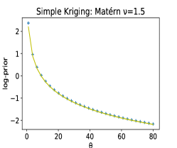
(a) Line: $-\log(\theta)+2.2$

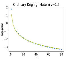
(b) Line: $-\log(\theta)+1.1$

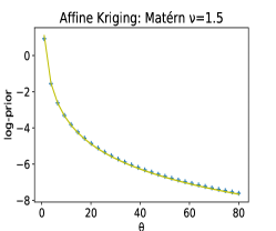
(c) Line: $-2\log(\theta)+1.1$

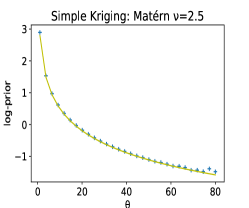
(d) Line: $-\log(\theta)+2.8$

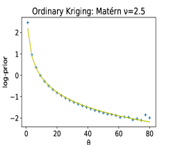
(e) Line: $-\log(\theta)+2.2$

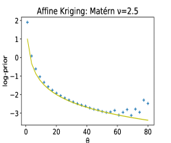
(f) Line: $-\log(\theta)+1.0$

Figure 1: Logarithm of the reference prior density for large values of $\theta$ for varying Kriging models and correlation kernels. In each case, the design space is one-dimensional ($r=1$) and the design set is the 10-point regular grid on $[0,1]$.

Figure 1 is consistent with the bound for tail rates given in Proposition 4.1.

For rough kernels (Spherical, Power Exponential with $\rho<2$, Matérn with $\nu<1$), Berger, De Oliveira and Sansó (2001) prove that if $\boldsymbol{1}$ belongs to the vector space spanned by the columns of $\boldsymbol{H}$ (as happens in Ordinary and Affine Kriging), then the reference prior is proper.

The upper bound provided by Proposition 4.1, $O(\theta^{-1})$, can be tightened in some cases. For example, in the case of Affine Kriging with a Matérn kernel with smoothness $\nu=1.5$ (figure 1c), the prior is bounded by $O(\theta^{-2})$. See Proposition B.1 in Appendix B for a proof.

The following lemma deals with the asymptotic behavior of the integrated likelihood when $\theta\to+\infty$.

Let $v_{1}(\theta)\geqslant...\geqslant v_{n-p}(\theta)>0$ be the ordered eigenvalues of $\boldsymbol{W}^{\top}\boldsymbol{\Sigma}_{\theta}\boldsymbol{W}$.

Lemma 4.2.

For Rational Quadratic and Squared Exponential kernels and for Matérn kernels with smoothness $\nu\geqslant 1$, there exists a hyperplane $\mathcal{H}_{n}$ of $\mathbb{R}^{n}$ such that for every $\boldsymbol{y}\in\mathbb{R}^{n}\setminus\mathcal{H}_{n}$, when $\theta\to+\infty$:

$$\left(\boldsymbol{y}^{\top}\boldsymbol{W}\left(\boldsymbol{W}^{\top}\boldsymbol{\Sigma}_{\theta}\boldsymbol{W}\right)^{-1}\boldsymbol{W}^{\top}\boldsymbol{y}\right)^{-1}=O(v_{n-p}(\theta)).$$ (4.3)

In particular, in the case of Simple Kriging, $\boldsymbol{W}$ is the identity matrix and $p=0$:

$$\left(\boldsymbol{y}^{\top}\boldsymbol{\Sigma}_{\theta}^{-1}\boldsymbol{y}\right)^{-1}=O(v_{n}(\theta)).$$ (4.4)

The proof of this lemma can be found in Appendix A.5.

For $\boldsymbol{y}\notin\mathcal{H}_{n}$, Lemma 4.2 shows that the smallest eigenvalue $v_{n-p}(\theta)$ of $\boldsymbol{W}^{\top}\boldsymbol{\Sigma}_{\theta}\boldsymbol{W}$ is an asymptotic upper bound for one of the factors of the squared integrated likelihood $L_{\boldsymbol{y}}(\theta)^{2}$ when $\theta\to+\infty$.

We need to take the other factors into account in order to obtain an asymptotic upper bound of the squared integrated likelihood. Combined with Proposition 2.2, Lemma 4.2 implies the following result.

Proposition 4.3.

If the observation vector $\boldsymbol{y}$ belongs to $\mathbb{R}^{n}\setminus\mathcal{H}_{n}$ ($\mathcal{H}_{n}$ is defined in Lemma 4.2), then

$$L_{\boldsymbol{y}}(\theta)^{2}=\prod_{i=1}^{n-p}\frac{O(v_{n-p}(\theta))}{v_{i}(\theta)}\quad\mathit{when}\;\theta\to+\infty.$$ (4.5)

Notice that all factors in the product (4.5) are $O(1)$ when $\theta\to+\infty$. For $\boldsymbol{y}\notin\mathcal{H}_{n}$, Proposition 4.3 thus implies the existence of a constant asymptotic upper bound for the likelihood $L_{\boldsymbol{y}}(\theta)$. It does not provide any tighter explicit upper bound, and this bound can only guarantee posterior propriety if the prior is itself proper (cf. Remark 2). However, it provides an implicit upper bound that will be used in proofs of posterior propriety.

For $\boldsymbol{y}\notin\mathcal{H}_{n}$, when $\theta\to+\infty$, any upper bound of the ratio $\frac{v_{n-p}(\theta)}{v_{1}(\theta)}$ is an upper bound of the squared likelihood $L_{\boldsymbol{y}}(\theta)^{2}$.

Figure 2 in Appendix B gives an idea of the explicit tail rates of the marginal log-likelihood in several situations.

Theorem 4.4.

For Rational Quadratic kernels and Squared Exponential kernels and for any Matérn kernel with smoothness $\nu\geqslant 1$, there exists a hyperplane $\mathcal{H}_{n}$ of $\mathbb{R}^{n}$ such that if $\boldsymbol{y}$ belongs to $\mathbb{R}^{n}\setminus\mathcal{H}_{n}$, then the reference posterior distribution $\pi(\theta|\boldsymbol{y})$ is proper.

Remark 3.

The requirement that $\boldsymbol{y}$ should belong to $\mathbb{R}^{n}\setminus\mathcal{H}_{n}$ is not substantially restrictive. If $\boldsymbol{y}$ is actually sampled from a nondegenerate Gaussian process, it almost surely does not belong to the hyperplane $\mathcal{H}_{n}$. Therefore, if $\boldsymbol{y}$ actually does belong to $\mathcal{H}_{n}$, it might be better explained by a degenerate Gaussian model. The most compelling example is that of a constant observation vector, for which the Kriging model would be grossly inappropriate. In case there is some doubt about whether a given $\boldsymbol{y}$ belongs to $\mathbb{R}^{n}\setminus\mathcal{H}_{n}$, Appendix A.7 provides explicit sufficient conditions instead.

The proof of the Theorem can be found in Appendix A.6.

Depending on the matrix $\boldsymbol{H}$ (or its absence in the case of Simple Kriging), the bounds of the likelihood function may differ. In some cases, it is even possible to derive a tighter bound for the prior than the general one given in Proposition 4.1. Examples are given in Appendix B: Affine Kriging with a Matérn kernel with smoothness $\nu\in[1,2)$ (Propositions B.1 and B.2) and Ordinary Kriging with a Matérn kernel with smoothness $\nu=1$ (Proposition B.3).

5 Conclusion

In this work, we proved that for a large class of smooth kernels, the reference prior leads to a proper posterior distribution. This class contains the Squared Exponential correlation kernel as well as the important Matérn family (Stein, 1999) with smoothness parameter $\nu\geqslant 1$. The seldom used Rational Quadratic kernels are also included within this class.

Berger, De Oliveira and Sansó (2001) proved this result for a class of rough correlation kernels. This class includes the complementary set of the Matérn family – kernels with smoothness parameter $\nu<1$ – as well as all other Power Exponential kernels. Spherical kernels, which are mostly used in the field of geostatistics also belong to this class.

The results from Berger, De Oliveira and Sansó (2001), together with Theorem 4.4, show how polyvalent the reference prior is, insofar as it is able to adapt to very different correlation kernels and always leads to a proper posterior. The key to this flexibility is the way the tail rate of the reference prior adapts to the tail rate of the integrated likelihood, which depends on the correlation matrix $\boldsymbol{\Sigma}_{\theta}$ and the trend matrix $\boldsymbol{H}$. For rough correlation kernels, Berger, De Oliveira and Sansó (2001) were able to express likelihood tail rates as an explicit function of $\theta$. More research is needed to do the same for smoother correlation kernels, even though Appendix B provides explicit tail rates in a few specific cases.

The reference prior’s flexilibility means no ad-hoc technique is required to derive useable inference. This makes the approach appealing from a Bayesian point of view when no explicit prior information is available. Even when explicit prior information is available, following Druilhet and Marin (2007), the reference prior can be used to derive maximum a posteriori (MAP) estimates or High Probability Density (HPD) sets that are invariant under reparametrization.

In Section 3, we recalled that the original proof from Berger, De Oliveira and Sansó (2001) relies on the matrix $\boldsymbol{D}^{(q)}$ from the Taylor expansion of the correlation matrix being nonsingular (cf. Proposition 3.1). Provided there are enough observation points, this implies that $q<1$. Stein (1999) shows that the correlation kernel cannot then be twice continously differentiable at 0 (p. 28, section “Principal irregular term”).

Since they make the same assumption, this restriction to rough correlation kernels also applies to all works generalizing the original result from Berger, De Oliveira and Sansó (2001). Gu, Wang and Berger (2018) provide the largest generalization to date: their setting admits anisotropic kernels defined as products of one-dimensional kernels and a possible additional noise term (nugget effect). It does not admit anisotropic geometric kernels, however (see Table 3 for a definition). They prove that one of the reference priors leads to a proper posterior: the prior derived from the reference prior algorithm where $\boldsymbol{\beta}$ is the lower-ranking parameter and $\sigma^{2}$, $\boldsymbol{\theta}=(\theta_{1},...,\theta_{r})$ and possibly the parameter controlling the nugget effect are collectively the higher-ranking group of parameters. Like Berger, De Oliveira and Sansó (2001), they assume that the matrix $\boldsymbol{D}^{(q)}$ from Proposition 3.1 is nonsingular regardless of $q$, so their proof applies to products of rough correlation kernels (Spherical, Power Exponential with $\rho<2$ and Matérn with $\nu<1$). Unfortunately, the proof used in the present article to deal with smoother kernels (Rational Quadratic, Squared Exponential and Matérn with $\nu\geqslant 1$) cannot easily be adjusted to their setting. The corresponding reference prior is indeed much more complex as it is proportional to the square root of the Fisher information matrix of either $r+1$ parameters ($\sigma^{2},\theta_{1},...,\theta_{r}$) or $r+2$ parameters if there is a nugget effect.

Correlation lengths	Product	Anisotropic geometric
$\boldsymbol{\theta}=(\theta_{1},...,\theta_{r})$	$\prod_{i=1}^{r}K_{\theta_{i}}(t_{i})$	$K_{1}\left(\left(\sum_{i=1}^{r}\frac{t_{i}^{2}}{\theta_{i}^{2}}\right)^{1/2}\right)$

Table 3: Anisotropic correlation kernels. $K_{\theta}$ is a 1-dimensional kernel with correlation length $\theta$.

Whenever the reference posterior is known to be proper – whether in the case of isotropic correlation kernels as shown in the present article or in the case of a product of rough correlation kernels as shown in Gu, Wang and Berger (2018) – it is theoretically possible to propagate parameter uncertainty to the predictions of the Gaussian process model. This can be done through Markov Chain Monte-Carlo (MCMC) sampling of the marginal reference posterior distribution on $\boldsymbol{\theta}$. The spread of the predictions obtained using the different values of $\boldsymbol{\theta}$ account for parameter uncertainty: not only the uncertainty on $\boldsymbol{\theta}$, but also on $\boldsymbol{\beta}$ and $\sigma^{2}$ since the latter can be marginalized out of the model (cf. Proposition 2.2). In practice though, Gu, Wang and Berger (2018) do not advocate this method because of the computational cost of MCMC in this setting. They use the maximum a posteriori (MAP) estimate for $\boldsymbol{\theta}$ instead. This effectively means that the density of the reference posterior distribution acts as a penalization factor on the likelihood. An alternative proposal is to sample the $\theta_{i}$ ($1\leqslant i\leqslant r$) from one-dimensional reference posterior distributions in order to make MCMC tractable (Muré, 2019).

Appendix A Proofs

The proofs presented in this Appendix rely on auxiliary facts from Appendix C. Appendix C can be found in supplementary material.

A.1 Proof of Proposition 2.1

Proof.

Both assertions follow from results proved by Ren, Sun and He (2012). The first follows from their Proposition 5 (a) (taken in the particular case with no nugget effect). The second is a consequence of Lemma C.1, which restates their Lemma 6: it implies that

$$\boldsymbol{W}\left(\boldsymbol{W}^{\top}\boldsymbol{\Sigma}_{\theta}\boldsymbol{W}\right)^{-1}\boldsymbol{W}^{\top}=\boldsymbol{\Sigma}_{\theta}^{-1}\left(\boldsymbol{I}_{n}-\boldsymbol{H}\left(\boldsymbol{H}^{\top}\boldsymbol{\Sigma}_{\theta}^{-1}\boldsymbol{H}\right)^{-1}\boldsymbol{H}^{\top}\boldsymbol{\Sigma}_{\theta}^{-1}\right).$$ (A.1)

∎

A.2 Proof of Proposition 2.2

Proof.

The result for $p=0$ and the first result for $p\geqslant 1$ are from Berger, De Oliveira and Sansó (2001).

From (A.1), all that remains to be proved is the determinant equality $\left|\boldsymbol{\Sigma}_{\theta}\right|=\left|\boldsymbol{W}^{\top}\boldsymbol{\Sigma}_{\theta}\boldsymbol{W}\right|\left|\boldsymbol{H}^{\top}\boldsymbol{H}\right|\left|\boldsymbol{H}^{\top}\boldsymbol{\Sigma}_{\theta}^{-1}\boldsymbol{H}\right|^{-1}$. Choose an $n\times p$ matrix $\boldsymbol{P}$ with columns forming an orthonormal basis of the $p$-dimensional subspace of $\mathbb{R}^{n}$ spanned by the columns of $\boldsymbol{H}$. Let $(\boldsymbol{W}\boldsymbol{P})$ denote the matrix whose left $n\times(n-p)$ block is $\boldsymbol{W}$ and whose right $n\times p$ block is $\boldsymbol{P}$. $(\boldsymbol{W}\boldsymbol{P})$ is an $n\times n$ orthogonal matrix, so we have $\left|\boldsymbol{\Sigma}_{\theta}\right|=\left|(\boldsymbol{W}\boldsymbol{P})^{\top}\boldsymbol{\Sigma}_{\theta}(\boldsymbol{W}\boldsymbol{P})\right|$. Using Schur’s complement (see for example Serre (2002) p. 139),

$$\left|\boldsymbol{\Sigma}_{\theta}\right|=\left|\boldsymbol{W}^{\top}\boldsymbol{\Sigma}_{\theta}\boldsymbol{W}\right|\left|\boldsymbol{P}^{\top}\boldsymbol{\Sigma}_{\theta}\left(\boldsymbol{I}_{n}-\boldsymbol{W}\left(\boldsymbol{W}^{\top}\boldsymbol{\Sigma}_{\theta}\boldsymbol{W}\right)^{-1}\boldsymbol{W}^{\top}\boldsymbol{\Sigma}_{\theta}\right)\boldsymbol{P}\right|.$$ (A.2)

Equation (A.1) is equivalent to:

$$\boldsymbol{\Sigma}_{\theta}\left(\boldsymbol{I}_{n}-\boldsymbol{W}\left(\boldsymbol{W}^{\top}\boldsymbol{\Sigma}_{\theta}\boldsymbol{W}\right)^{-1}\boldsymbol{W}^{\top}\boldsymbol{\Sigma}_{\theta}\right)=\boldsymbol{H}\left(\boldsymbol{H}^{\top}\boldsymbol{\Sigma}_{\theta}^{-1}\boldsymbol{H}\right)^{-1}\boldsymbol{H}^{\top}.$$ (A.3)

Plugging this in Equation (A.2), we obtain:

$$\left|\boldsymbol{\Sigma}_{\theta}\right| =\left|\boldsymbol{W}^{\top}\boldsymbol{\Sigma}_{\theta}\boldsymbol{W}\right|\left|\boldsymbol{P}^{\top}\boldsymbol{H}\right|^{2}\left|\boldsymbol{H}^{\top}\boldsymbol{\Sigma}_{\theta}^{-1}\boldsymbol{H}\right|$$

$$=\left|\boldsymbol{W}^{\top}\boldsymbol{\Sigma}_{\theta}\boldsymbol{W}\right|\left|\boldsymbol{H}^{\top}\underbrace{\boldsymbol{P}\boldsymbol{P}^{\top}}_{\boldsymbol{I}_{p}}\boldsymbol{H}\right|\left|\boldsymbol{H}^{\top}\boldsymbol{\Sigma}_{\theta}^{-1}\boldsymbol{H}\right|.$$ (A.4)

∎

A.3 Proof of Proposition 3.1

Proof.

Let us consider the $(i,i^{\prime})$-th element of the matrix $\boldsymbol{\Sigma}_{\theta}$. Letting $K_{\theta}$ denote the correlation kernel, it is given by $K_{\theta}\left(\boldsymbol{x}^{(i)}-\boldsymbol{x}^{(i^{\prime})}\right)$.

1. With a spherical kernel,

$$K_{\theta}\left(\boldsymbol{x}^{(i)}-\boldsymbol{x}^{(i^{\prime})}\right):=1-\frac{3}{2}\frac{\left\|\boldsymbol{x}^{(i)}-\boldsymbol{x}^{(i^{\prime})}\right\|}{\theta}+\frac{1}{2}\frac{\left\|\boldsymbol{x}^{(i)}-\boldsymbol{x}^{(i^{\prime})}\right\|^{3}}{\theta^{3}}.$$ (A.5)

We can identify $g_{0}(\theta)$ as $-(3/2)\theta^{-1}$, $q$ as $1/2$ and $\boldsymbol{R}_{0}(\theta)$ as the matrix whose $(i,j)$-th element is $\frac{1}{2}\frac{\left\|\boldsymbol{x}^{(i)}-\boldsymbol{x}^{(i^{\prime})}\right\|^{3}}{\theta^{3}}$.

2. With a Power Exponential kernel,

$$K_{\theta}\left(\boldsymbol{x}^{(i)}-\boldsymbol{x}^{(i^{\prime})}\right):=\exp\left(-\frac{\left\|\boldsymbol{x}^{(i)}-\boldsymbol{x}^{(i^{\prime})}\right\|^{\rho}}{\theta^{\rho}}\right).$$ (A.6)

When $\theta\to+\infty$,

$$K_{\theta}\left(\boldsymbol{x}^{(i)}-\boldsymbol{x}^{(i^{\prime})}\right)=1-\frac{\left\|\boldsymbol{x}^{(i)}-\boldsymbol{x}^{(i^{\prime})}\right\|^{\rho}}{\theta^{\rho}}+O\left(\theta^{-2\rho}\right).$$ (A.7)

We can identify $g_{0}(\theta)$ as $-\theta^{-\rho}$ and $q$ as $\rho/2$. Then $\left\|\boldsymbol{R}_{0}(\theta)\right\|=O(\theta^{-2\rho})$ when $\theta\to\infty$.

3. With a Rational Quadratic kernel,

$$K_{\theta}\left(\boldsymbol{x}^{(i)}-\boldsymbol{x}^{(i^{\prime})}\right):=\left(1+\frac{\left\|\boldsymbol{x}^{(i)}-\boldsymbol{x}^{(i^{\prime})}\right\|^{2}}{\theta^{2}}\right)^{-\nu}.$$ (A.8)

When $\theta\to+\infty$,

$$K_{\theta}\left(\boldsymbol{x}^{(i)}-\boldsymbol{x}^{(i^{\prime})}\right)=1-\nu\frac{\left\|\boldsymbol{x}^{(i)}-\boldsymbol{x}^{(i^{\prime})}\right\|^{2}}{\theta^{2}}+O(\theta^{-4}).$$ (A.9)

We can identify $g_{0}(\theta)$ as $-\nu\theta^{-2}$ and $q$ as $1$. Then $\left\|\boldsymbol{R}_{0}(\theta)\right\|=O(\theta^{-4})$ when $\theta\to\infty$.

4. With a Matérn kernel, we only need to refer to the appropriate decomposition of $\boldsymbol{\Sigma}_{\theta}$ in Appendix C.4 (Lemma C.15 if $\nu$ is no integer and Lemma C.17 if $\nu$ is an integer) to identify $g_{0}(\theta)$, $\boldsymbol{D}^{(q)}$ and obtain the relevant properties for $\boldsymbol{R}_{0}(\theta)=\boldsymbol{\Sigma}_{\theta}-\boldsymbol{11}^{\top}-g_{0}(\theta)\boldsymbol{D}^{(q)}$.

• If $\nu<1$:

  • $g_{0}(\theta)=\Gamma(-\nu)\nu^{\nu}/(\Gamma(\nu)\theta^{2\nu})$;

  • $q=\nu$;

  • $\|\boldsymbol{R}(\theta)\|=O(\theta^{-2})=o(g_{0}(\theta))$ when $\theta\to\infty$.

• If $\nu=1$:

  • $g_{0}(\theta)=-2\log(\theta)/\theta^{2}$;

  • $q=1$;

  • $\|\boldsymbol{R}(\theta)\|=O(\theta^{-2})=o(g_{0}(\theta))$ when $\theta\to\infty$.

• If $\nu>1$:

  • $g_{0}(\theta)=-\nu(\nu-1)^{-1}/\theta^{2}$;

  • $q=1$;

  • $\|\boldsymbol{R}(\theta)\|=O(\theta^{-2\min(2,\nu)})=o(g_{0}(\theta))$ when $\theta\to\infty$.

∎

A.4 Proof of Proposition 4.1

Proof.

When $\theta\to 0$, $\boldsymbol{\Sigma}_{\theta}$ converges to $\boldsymbol{I}_{n}$, so its inverse does too. Therefore, in order to prove the first assertion, it is enough to prove that $\left\|\frac{d}{d\theta}\boldsymbol{\Sigma}_{\theta}\right\|=o(1)$ for Matérn ($\nu\geqslant 1$) and Squared Exponential kernels and that $\left\|\frac{d}{d\theta}\boldsymbol{\Sigma}_{\theta}\right\|=O(\theta^{2\nu-1})$ for Rational Quadratic kernels. To do this, we prove that these bounds hold for every element of the matrix $\frac{d}{d\theta}\boldsymbol{\Sigma}_{\theta}$.

Letting $K_{\theta}$ be one of the considered kernels, the $(i,i^{\prime})$-th element of $\frac{d}{d\theta}\boldsymbol{\Sigma}_{\theta}$ is given by $\frac{d}{d\theta}K_{\theta}\left(\left\|\boldsymbol{x}^{(i)}-\boldsymbol{x}^{(i^{\prime})}\right\|\right)$.

If $K_{\theta}$ is Squared Exponential, $\lim_{\theta\to 0}\frac{d}{d\theta}K_{\theta}\left(\left\|\boldsymbol{x}^{(i)}-\boldsymbol{x}^{(i^{\prime})}\right\|\right)=0$. This also holds if $K_{\theta}$ is a Matérn kernel with smoothness $\nu\geqslant 1$ (see Abramowitz and Stegun (1964) 9.6.28. and 9.7.2.).

If $K_{\theta}$ is a Rational Quadratic kernel with parameter $\nu>0$, then when $\theta\to 0$, $\frac{d}{d\theta}K_{\theta}\left(\left\|\boldsymbol{x}^{(i)}-\boldsymbol{x}^{(i^{\prime})}\right\|\right)/\theta^{2\nu-1}$ admits a finite limit.

Let us prove the second assertion.

Lemma C.20 shows that for Matérn kernels with smoothness $\nu$, for all $\theta>0$ and all $\boldsymbol{\xi}\in\mathbb{R}^{n}$:

$$0\leqslant\boldsymbol{\xi}^{\top}\left(r\theta^{-1}\boldsymbol{\Sigma}_{\theta}-\frac{d}{d\theta}\boldsymbol{\Sigma}_{\theta}\right)\boldsymbol{\xi}\leqslant(2\nu+r)\theta^{-1}\boldsymbol{\xi}^{\top}\boldsymbol{\Sigma}_{\theta}\boldsymbol{\xi}.$$ (A.10)

Because of this, Lemma C.3 yields an upper bound on the reference prior density:

$$\begin{split}&\sqrt{\operatorname{Tr}\left[\left\{\left(\frac{d}{d\theta}\boldsymbol{\Sigma}_{\theta}\right)\boldsymbol{\Sigma}_{\theta}^{-1}\boldsymbol{Q}_{\theta}\right\}^{2}\right]-\frac{1}{n-p}\left[\operatorname{Tr}\left\{\left(\frac{d}{d\theta}\boldsymbol{\Sigma}_{\theta}\right)\boldsymbol{\Sigma}_{\theta}^{-1}\boldsymbol{Q}_{\theta}\right\}\right]^{2}}\\ \leqslant&(n-p)(2\nu+r)\theta^{-1}.\end{split}$$ (A.11)

For Squared Exponential and Rational Quadratic kernels, a similar proof is possible. Lemma C.19 implies that there exists a positive constant $C$ such that for large enough $\theta$, for all $\boldsymbol{\xi}\in\mathbb{R}^{n}$,

$$0\leqslant\boldsymbol{\xi}^{\top}\left(\theta^{-1}\boldsymbol{\Sigma}_{\theta}-\frac{d}{d\theta}\boldsymbol{\Sigma}_{\theta}\right)\boldsymbol{\xi}\leqslant C\theta^{-1}\boldsymbol{\xi}^{\top}\boldsymbol{\Sigma}_{\theta}\boldsymbol{\xi}.$$ (A.12)

Like in the Matérn case, Lemma C.3 shows that this implies an upper bound on the reference prior density:

$$\begin{split}&\sqrt{\operatorname{Tr}\left[\left\{\left(\frac{d}{d\theta}\boldsymbol{\Sigma}_{\theta}\right)\boldsymbol{\Sigma}_{\theta}^{-1}\boldsymbol{Q}_{\theta}\right\}^{2}\right]-\frac{1}{n-p}\left[\operatorname{Tr}\left\{\left(\frac{d}{d\theta}\boldsymbol{\Sigma}_{\theta}\right)\boldsymbol{\Sigma}_{\theta}^{-1}\boldsymbol{Q}_{\theta}\right\}\right]^{2}}\\ \leqslant&(n-p)C\theta^{-1}.\end{split}$$ (A.13)

∎

A.5 Proof of Lemma 4.2

Proof.

The kernel of a matrix $\boldsymbol{M}$ is denoted by $\operatorname{Ker}(\boldsymbol{M})$.

For Rational Quadratic and Squared Exponential kernels, Lemma C.13 provides an asymptotic expansion of $\boldsymbol{\Sigma}_{\theta}$. When $\theta$ is large enough,

$$\boldsymbol{\Sigma}_{\theta}=\sum_{k=0}^{\infty}\frac{a_{k}}{\theta^{2k}}\boldsymbol{D}^{(k)}.$$ (A.14)

In Equation (A.14), for every $k$, $\boldsymbol{D}^{(k)}$ is the $n\times n$ matrix with $(i,i^{\prime})$-th element $\|\boldsymbol{x}^{(i)}-\boldsymbol{x}^{(i^{\prime})}\|^{2k}$ and $a_{k}$ is a non-null real number that depends on the kernel.

Because $\boldsymbol{\Sigma}_{\theta}$ is nonsingular, the intersection $\cap_{k=0}^{\infty}\operatorname{Ker}\boldsymbol{D}^{(k)}$ is the trivial vector space, i.e. the vector space containing only the null vector. This means there must exist (cf. Lemma C.4) a nonnegative integer $k^{\prime}$ such that the vector space $\cap_{k=0}^{k^{\prime}}\operatorname{Ker}\left(\boldsymbol{W}^{\top}\boldsymbol{D}^{(k)}\boldsymbol{W}\right)$ is trivial and such that the vector space $\cap_{0\leqslant k<k^{\prime}}\operatorname{Ker}\left(\boldsymbol{W}^{\top}\boldsymbol{D}^{(k)}\boldsymbol{W}\right)$ is non-trivial (if $k^{\prime}=0$, the intersection is done over an empty index set, so we take it to be $\mathbb{R}^{n-p}$ by convention).

This implies (cf. Lemma C.6) that for any $\boldsymbol{y}^{\prime}\in\mathbb{R}^{n-p}$ that does not belong to the vector subspace $\mathcal{A}_{k^{\prime}-1}$ spanned by the columns of the matrices $\boldsymbol{W}^{\top}\boldsymbol{D}^{(k)}\boldsymbol{W}$ ($0\leqslant k\leqslant k^{\prime}-1$), there exists $c_{\boldsymbol{y}^{\prime}}>0$ such that for large enough $\theta$,

$$\left(\boldsymbol{y}^{\prime}\right)^{\top}\left(\boldsymbol{W}^{\top}\boldsymbol{\Sigma}_{\theta}\boldsymbol{W}\right)^{-1}\boldsymbol{y}^{\prime}\geqslant c_{\boldsymbol{y}^{\prime}}\left\|\left(\boldsymbol{W}^{\top}\boldsymbol{\Sigma}_{\theta}\boldsymbol{W}\right)^{-1}\right\|.$$ (A.15)

As a consequence, for every $\boldsymbol{y}\in\mathbb{R}^{n}$ such that $\boldsymbol{W}^{\top}\boldsymbol{y}\notin\mathcal{A}_{k^{\prime}-1}$, there exists $c_{\boldsymbol{y}}>0$ such that for large enough $\theta$,

$$\boldsymbol{y}^{\top}\boldsymbol{W}\left(\boldsymbol{W}^{\top}\boldsymbol{\Sigma}_{\theta}\boldsymbol{W}\right)^{-1}\boldsymbol{W}^{\top}\boldsymbol{y}\geqslant c_{\boldsymbol{y}}\left\|\left(\boldsymbol{W}^{\top}\boldsymbol{\Sigma}_{\theta}\boldsymbol{W}\right)^{-1}\right\|.$$ (A.16)

Let $\boldsymbol{W}\mathcal{A}_{k^{\prime}-1}$ denote the vector subspace of $\mathbb{R}^{n}$ of all vectors $\boldsymbol{v}\in\mathbb{R}^{n}$ such that $\boldsymbol{W}^{\top}\boldsymbol{v}$ does belong to $\mathcal{A}_{k^{\prime}-1}$. Because the matrix $\boldsymbol{W}^{\top}$ has full row rank, $\boldsymbol{W}\mathcal{A}_{k^{\prime}-1}$ is included within a hyperspace $\mathcal{H}_{n}$ of $\mathbb{R}^{n}$. Therefore, for every $\boldsymbol{y}\in\mathbb{R}^{n}\setminus\mathcal{H}_{n}$, there exists $c_{\boldsymbol{y}}>0$ such that for large $\theta$ the equation above holds.

For Matérn kernels with noninteger smoothness $\nu>0$ (resp. with integer smoothness $\nu>0$), Lemma C.15 (resp. Lemma C.17) allows a similar argument.

$$\boldsymbol{\Sigma}_{\theta} =\sum_{k=0}^{\left\lfloor\nu\right\rfloor}\frac{a_{k}}{\theta^{2k}}\boldsymbol{D}^{(k)}+\frac{a_{\nu}}{\theta^{2\nu}}\boldsymbol{D}^{(\nu)}+\boldsymbol{R}_{\nu}(\theta) \textrm{if }\nu\textrm{ is noninteger.}$$ (A.17)

$$\boldsymbol{\Sigma}_{\theta} =\sum_{k=0}^{\nu-1}\frac{a_{k}}{\theta^{2k}}\boldsymbol{D}^{(k)}+\tilde{a}_{\nu}\left(\frac{\log(\theta)}{\theta^{2\nu}}\boldsymbol{D}^{(\nu)}+\frac{1}{\theta^{2\nu}}\boldsymbol{\tilde{D}}^{(\nu)}\right)+\boldsymbol{\tilde{R}}_{\nu}(\theta) \textrm{if }\nu\textrm{ is an integer.}$$ (A.18)

In these expressions the $a_{k}$, $a_{\nu}$ and $\tilde{a}_{\nu}$ are non-null real numbers, for every $k$, $\boldsymbol{D}^{(k)}$ is the $n\times n$ matrix with $(i,i^{\prime})$-th element $\|\boldsymbol{x}^{(i)}-\boldsymbol{x}^{(i^{\prime})}\|^{2k}$, $\boldsymbol{D}^{(\nu)}$ is the $n\times n$ matrix with $(i,i^{\prime})$-th element $\|\boldsymbol{x}^{(i)}-\boldsymbol{x}^{(i^{\prime})}\|^{2\nu}$, $\boldsymbol{\tilde{D}}^{(\nu)}$ is another non-null symmetric $n\times n$ matrix, and $\boldsymbol{R}_{\nu}$ (resp.$\boldsymbol{\tilde{R}}_{\nu}$) is a function from $(0,+\infty)$ to the space of $n\times n$ matrices such that $\left\|\boldsymbol{R}(\nu)\right\|=o(\theta^{2\nu})$ (resp. $\left\|\boldsymbol{\tilde{R}}(\nu)\right\|=o(\theta^{2\nu})$) when $\theta\to+\infty$.

With Matérn kernels, when $\theta\to+\infty$, $\left\|\boldsymbol{\Sigma}_{\theta}^{-1}\right\|=O(\theta^{2\nu})$ (cf. Lemma C.11), so in the decomposition of $\boldsymbol{\Sigma}_{\theta}$ given by Equation (A.17) (resp. Equation (A.18)), the intersection $\cap_{k=0}^{\left\lfloor\nu\right\rfloor}\operatorname{Ker}\left(\boldsymbol{W}^{\top}\boldsymbol{D}^{(k)}\boldsymbol{W}\right)\cap\operatorname{Ker}\left(\boldsymbol{W}^{\top}\boldsymbol{D}^{(\nu)}\boldsymbol{W}\right)$ (resp. the intersection $\cap_{k=0}^{\nu}\operatorname{Ker}\left(\boldsymbol{W}^{\top}\boldsymbol{D}^{(k)}\boldsymbol{W}\right)\cap\operatorname{Ker}\left(\boldsymbol{W}^{\top}\boldsymbol{\tilde{D}}^{(\nu)}\boldsymbol{W}\right)$) is necessarily the trivial vector space.

The rest of the proof is the same as in the case of Rational Quadratic and Squared Exponential kernels.

∎

A.6 Proof of Theorem 4.4

Proof.

The first assertion of Proposition 4.1 implies the reference prior $\pi(\theta)$ is integrable in the neighborhood of 0. Furthermore, when $\theta\to 0$, $\boldsymbol{\Sigma}_{\theta}\to\boldsymbol{I}_{n}$ so the reference posterior $\pi(\theta|\boldsymbol{y})\propto L(\boldsymbol{y}|\theta)\pi(\theta)$ is integrable in the neighborhood of 0 as well.

All that remains to be proved is therefore that the reference posterior is integrable in the neighborhood of $+\infty$. In the following $\theta\to+\infty$, so we rely on the asymptotic expansion of $\boldsymbol{\Sigma}_{\theta}$ which is detailed in Appendix C.4.

Let $\mathcal{H}_{n}$ be the hyperplane of $\mathbb{R}^{n}$ defined by Lemma 4.2. Let us fix the observation vector $\boldsymbol{y}\in\mathbb{R}^{n}\setminus\mathcal{H}_{n}$.

The proof is somewhat trickier for Matérn kernels with integer smoothness, so we tackle this case at the end. Until further notice, assume the kernel is Rational Quadratic, Squared Exponential or Matérn with noninteger smoothness $\nu>1$.

A.6.1 Rational Quadratic, Squared Exponential and Matérn kernels with noninteger smoothness $\nu>1$

For Rational Quadratic and Squared Exponential (resp. Matérn with noninteger smoothness parameter $\nu>1$) kernels, Lemma C.14 (resp. Lemma C.16) shows how $\boldsymbol{W}^{\top}\boldsymbol{\Sigma}_{\theta}\boldsymbol{W}$ can be decomposed as

$$\boldsymbol{W}^{\top}\boldsymbol{\Sigma}_{\theta}\boldsymbol{W}=g(\theta)\left(\boldsymbol{W}^{\top}\boldsymbol{Z}\boldsymbol{W}+g^{\star}(\theta)\boldsymbol{W}^{\top}\boldsymbol{Z}^{\star}\boldsymbol{W}+\boldsymbol{R}_{g}(\theta)\right),$$ (A.19)

where:

• $g$ is a positive differentiable function on $(0,+\infty)$;

• $g^{\star}(\theta)=\theta^{-2l}$ with $l\in(0,+\infty)$ (actually, if the kernel is Rational Quadratic or Squared Exponential, $l\in\mathbb{Z}_{+}$);

• $\boldsymbol{R}_{g}$ is a differentiable function from $(0,+\infty)$ to $\mathcal{M}_{n}$ such that $\|\boldsymbol{R}_{g}(\theta)\|=o(g^{\star}(\theta))$ and $\|\frac{d}{d\theta}\boldsymbol{R}_{g}(\theta)\|=o(g^{\star\prime}(\theta))$;

• $\boldsymbol{Z}$ and $\boldsymbol{Z}^{\star}$ are both fixed symmetric matrices;

• $\boldsymbol{W}^{\top}\boldsymbol{Z}\boldsymbol{W}$ is non-null.

Remark 4.

Readers familiar with Berger, De Oliveira and Sansó (2001) may recognize similarities with the assumptions in Lemma 2 of the paper. This is not coincidental. The matrices $\boldsymbol{Z}$ and $\boldsymbol{Z}^{\star}$ essentially play the roles of the matrices $\boldsymbol{D}$ and $\boldsymbol{D}^{\star}$ respectively. However, $\boldsymbol{Z}$ (resp. $\boldsymbol{Z}^{\star}$) is not necessarily equal to $\boldsymbol{D}$ (resp. $\boldsymbol{D}^{\star}$). In fact, in the Simple Kriging case where $\boldsymbol{W}$ is the identity matrix, $\boldsymbol{Z}=\boldsymbol{1}\boldsymbol{1}^{\top}$.

Let us differentiate $\boldsymbol{W}^{\top}\boldsymbol{\Sigma}_{\theta}\boldsymbol{W}$:

$$\frac{d}{d\theta}\boldsymbol{W}^{\top}\boldsymbol{\Sigma}_{\theta}\boldsymbol{W}=\frac{g^{\prime}(\theta)}{g(\theta)}\boldsymbol{W}^{\top}\boldsymbol{\Sigma}_{\theta}\boldsymbol{W}+g(\theta)\left(g^{\star\prime}(\theta)\boldsymbol{W}^{\top}\boldsymbol{Z}^{\star}\boldsymbol{W}+\frac{d}{d\theta}\boldsymbol{R}_{g}(\theta)\right).$$ (A.20)

This decomposition of the matrix $\frac{d}{d\theta}\boldsymbol{W}^{\top}\boldsymbol{\Sigma}_{\theta}\boldsymbol{W}$ implies (cf. Lemma C.2) that it can be replaced in Equation (2.3) by $g(\theta)\left(g^{\star\prime}(\theta)\boldsymbol{W}^{\top}\boldsymbol{Z}^{\star}\boldsymbol{W}+\frac{d}{d\theta}\boldsymbol{R}_{g}(\theta)\right)$:

$$\begin{split}&\operatorname{Tr}\left[\left\{\left(\frac{g^{\prime}(\theta)}{g(\theta)}\boldsymbol{W}^{\top}\boldsymbol{\Sigma}_{\theta}\boldsymbol{W}+g(\theta)\left(g^{\star\prime}(\theta)\boldsymbol{W}^{\top}\boldsymbol{Z}^{\star}\boldsymbol{W}+\frac{d}{d\theta}\boldsymbol{R}_{g}(\theta)\right)\right)\left(\boldsymbol{W}^{\top}\boldsymbol{\Sigma}_{\theta}\boldsymbol{W}\right)^{-1}\right\}^{2}\right]\\ &-\frac{1}{n-p}\left[\operatorname{Tr}\left\{\left(\frac{g^{\prime}(\theta)}{g(\theta)}\boldsymbol{W}^{\top}\boldsymbol{\Sigma}_{\theta}\boldsymbol{W}+g(\theta)\left(g^{\star\prime}(\theta)\boldsymbol{W}^{\top}\boldsymbol{Z}^{\star}\boldsymbol{W}+\frac{d}{d\theta}\boldsymbol{R}_{g}(\theta)\right)\right)\left(\boldsymbol{W}^{\top}\boldsymbol{\Sigma}_{\theta}\boldsymbol{W}\right)^{-1}\right\}\right]^{2}\\ =&\operatorname{Tr}\left[\left\{g(\theta)\left(g^{\star\prime}(\theta)\boldsymbol{W}^{\top}\boldsymbol{Z}^{\star}\boldsymbol{W}+\frac{d}{d\theta}\boldsymbol{R}_{g}(\theta)\right)\left(\boldsymbol{W}^{\top}\boldsymbol{\Sigma}_{\theta}\boldsymbol{W}\right)^{-1}\right\}^{2}\right]\\ &-\frac{1}{n-p}\left[\operatorname{Tr}\left\{g(\theta)\left(g^{\star\prime}(\theta)\boldsymbol{W}^{\top}\boldsymbol{Z}^{\star}\boldsymbol{W}+\frac{d}{d\theta}\boldsymbol{R}_{g}(\theta)\right)\left(\boldsymbol{W}^{\top}\boldsymbol{\Sigma}_{\theta}\boldsymbol{W}\right)^{-1}\right\}\right]^{2}\\ \end{split}$$ (A.21)

So $\pi(\theta)\propto w(\theta)$, where

$$\begin{split}w(\theta)^{2}:=&\operatorname{Tr}\left[\left\{g(\theta)\left(g^{\star\prime}(\theta)\boldsymbol{W}^{\top}\boldsymbol{Z}^{\star}\boldsymbol{W}+\frac{d}{d\theta}\boldsymbol{R}_{g}(\theta)\right)\left(\boldsymbol{W}^{\top}\boldsymbol{\Sigma}_{\theta}\boldsymbol{W}\right)^{-1}\right\}^{2}\right]\\ &\quad-\frac{1}{n-p}\left[\operatorname{Tr}\left\{g(\theta)\left(g^{\star\prime}(\theta)\boldsymbol{W}^{\top}\boldsymbol{Z}^{\star}\boldsymbol{W}+\frac{d}{d\theta}\boldsymbol{R}_{g}(\theta)\right)\left(\boldsymbol{W}^{\top}\boldsymbol{\Sigma}_{\theta}\boldsymbol{W}\right)^{-1}\right\}\right]^{2}.\end{split}$$ (A.22)

We have $w(\theta)\leqslant\tilde{w}(\theta)$, where

$$\tilde{w}(\theta):=\sqrt{\operatorname{Tr}\left[\left\{g(\theta)\left(g^{\star\prime}(\theta)\boldsymbol{W}^{\top}\boldsymbol{Z}^{\star}\boldsymbol{W}+\frac{d}{d\theta}\boldsymbol{R}_{g}(\theta)\right)\left(\boldsymbol{W}^{\top}\boldsymbol{\Sigma}_{\theta}\boldsymbol{W}\right)^{-1}\right\}^{2}\right]}.$$ (A.23)

If $\boldsymbol{W}^{\top}\boldsymbol{Z}\boldsymbol{W}$ is nonsingular, then $\tilde{w}(\theta)=O(g^{\star\prime}(\theta))$. This implies $\pi(\theta)=O(g^{\star\prime}(\theta))=O(\theta^{-2l-1})$, so the reference prior is proper. The likelihood function is bounded due to Proposition 4.3, so the reference posterior is proper.

Remark 5.

Recall the decomposition of $\boldsymbol{\Sigma}_{\theta}$ from either Proposition 3.1 or Appendix A.5. If the vector $\boldsymbol{1}$ is one of the columns of $\boldsymbol{H}$, then we have $\boldsymbol{W}^{\top}\boldsymbol{D}^{(0)}\boldsymbol{W}=\boldsymbol{W}^{\top}\boldsymbol{11}^{\top}\boldsymbol{W}=\boldsymbol{0}$. Berger, De Oliveira and Sansó (2001) assume that the matrix $\boldsymbol{D}^{(1)}$ is necessarily nonsingular, which implies that $\boldsymbol{W}^{\top}\boldsymbol{D}^{(1)}\boldsymbol{W}$ is non-null (and thus equal to $\boldsymbol{W}^{\top}\boldsymbol{Z}\boldsymbol{W}$) and even nonsingular, so the paragraph above is applicable. This is why they reach the conclusion that the reference prior is proper as soon as $\boldsymbol{1}$ is one of the columns of $\boldsymbol{H}$ (denoted by $X$ in their article). Because the underlying assumption that $\boldsymbol{D}^{(1)}$ is nonsingular does not generally hold (cf. Proposition 3.4), there is reason to doubt the conclusion. Indeed, Figures 1b, 1e and 1f do not seem to support the claim.

If $\boldsymbol{W}^{\top}\boldsymbol{Z}\boldsymbol{W}$ is singular, Proposition 4.1 still ensures that $\pi(\theta)=O(\theta^{-1})$. Moreover, for any non-null vector $\boldsymbol{\xi}\in\mathbb{R}^{n-p}$ that belongs to the kernel of $\boldsymbol{W}^{\top}\boldsymbol{Z}\boldsymbol{W}$, $\boldsymbol{\xi}^{\top}\boldsymbol{W}^{\top}\boldsymbol{\Sigma}_{\theta}\boldsymbol{W}\boldsymbol{\xi}=O(g(\theta)g^{\star}(\theta))$. A fortiori, $v_{n-p}(\theta)=O(g(\theta)g^{\star}(\theta))$. As the rank of $\boldsymbol{W}^{\top}\boldsymbol{Z}\boldsymbol{W}$ is at least one, $v_{1}(\theta)^{-1}=O(g(\theta)^{-1})$. Gathering this, $v_{n-p}(\theta)/v_{1}(\theta)=O(g^{\star}(\theta))$. Proposition 4.3 implies that $L_{\boldsymbol{y}}(\theta)=O(g^{\star}(\theta))^{1/2})=O(\theta^{-l})$. The reference posterior is proportional to $L_{\boldsymbol{y}}(\theta)\pi(\theta)=O(\theta^{-l-1})$ and is proper.

A.6.2 Matérn kernels with integer smoothness $\nu$

We now address the case where the correlation kernel is Matérn with integer smoothness $\nu$. The proof strategy remains the same as for the other kernels, but the execution is a little trickier.

$\boldsymbol{D}^{(\nu)}$ is the $n\times n$ matrix with $(i,i^{\prime})$-th element $\|\boldsymbol{x}^{(i)}-\boldsymbol{x}^{(i^{\prime})}\|^{2\nu}$. Let $\boldsymbol{\tilde{D}}^{(\nu)}$ denote the $n\times n$ matrix with null diagonal and $(i,i^{\prime})$-th element ($i\neq i^{\prime}$) given by

$$\|\boldsymbol{x}^{(i)}-\boldsymbol{x}^{(i^{\prime})}\|^{2\nu}\left\{-\log\left(\|\boldsymbol{x}^{(i)}-\boldsymbol{x}^{(i^{\prime})}\|\right)-\frac{\log(\nu)}{2}-\gamma+\sum_{l=1}^{\nu}\frac{1}{2l}\right\},$$

where $\gamma$ is Euler’s constant.

Both $\boldsymbol{D}^{(\nu)}$ and $\boldsymbol{\tilde{D}}^{(\nu)}$ can appear in the decomposition of $\boldsymbol{W}^{\top}\boldsymbol{\Sigma}_{\theta}\boldsymbol{W}$ provided by Lemma C.18:

$$\boldsymbol{W}^{\top}\boldsymbol{\Sigma}_{\theta}\boldsymbol{W}=g(\theta)\left(\boldsymbol{W}^{\top}\boldsymbol{Z}\boldsymbol{W}+g^{\star}(\theta)\boldsymbol{W}^{\top}\boldsymbol{Z}^{\star}\boldsymbol{W}+\boldsymbol{R}_{g}(\theta)\right),$$ (A.24)

where:

• $g$ is a positive differentiable function on $(1,+\infty)$;

• $\boldsymbol{Z}$ and $\boldsymbol{Z}^{\star}$ are both fixed symmetric matrices;

• $\boldsymbol{W}^{\top}\boldsymbol{Z}\boldsymbol{W}$ is non-null;

• $g^{\star}(\theta)=\log(\theta)^{-1}$ if there exist non-null real numbers $\lambda,\lambda^{\star}$ such that $\boldsymbol{Z}=\lambda\boldsymbol{D}^{(\nu)}$ and $\boldsymbol{Z}^{\star}=\lambda^{\star}\boldsymbol{\tilde{D}}^{(\nu)}$;

• $g^{\star}(\theta)=\theta^{-2l}$ or $g^{\star}(\theta)=\log(\theta)\theta^{-2l}$ with $l\in(0,+\infty)$ otherwise;

• $\boldsymbol{R}_{g}$ is a differentiable function from $(0,+\infty)$ to $\mathcal{M}_{n}$ such that $\|\boldsymbol{R}_{g}(\theta)\|=o(g^{\star}(\theta))$ and $\|\frac{d}{d\theta}\boldsymbol{R}_{g}(\theta)\|=o(g^{\star\prime}(\theta))$ when $\theta\to+\infty$.

First, assume either that for all $\lambda\neq 0$, $\boldsymbol{Z}\neq\lambda\boldsymbol{D}^{(\nu)}$ or that for all $\lambda^{\star}\neq 0$, $\boldsymbol{Z}^{\star}\neq\lambda^{\star}\tilde{\boldsymbol{D}}^{(\nu)}$.

In Equation (A.19), according to Lemma C.18, $g^{\star}(\theta)$ may be $\theta^{-2l}\log(\theta)$ instead of $\theta^{-2l}$. If $g^{\star}(\theta)=\theta^{-2l}$ for some $l\in(0,+\infty)$, then the proof is the same as for Rational Quadratic, Squared Exponential and Matérn kernels with noninteger $\nu$. Assume therefore that $g^{\star}(\theta)=\theta^{-2l}\log(\theta)$ for some $l\in(0,+\infty)$. Then its derivative is $g^{\star\prime}(\theta)=\theta^{-2l-1}(1-2l\log(\theta))$.

If $\boldsymbol{W}^{\top}\boldsymbol{Z}\boldsymbol{W}$ is nonsingular, then the reference prior distribution is proper since $\pi(\theta)=O(g^{\star\prime}(\theta))=O(\theta^{-2l-1}\log(\theta))$. Proposition 4.3 guarantees that the likelihood function is bounded and therefore that the reference posterior is proper.

If $\boldsymbol{W}^{\top}\boldsymbol{Z}\boldsymbol{W}$ is singular, Proposition 4.1 still ensures that the reference prior is $O(\theta^{-1})$. Given the rank of $\boldsymbol{W}^{\top}\boldsymbol{Z}\boldsymbol{W}$ is at least one, $v_{n-p}(\theta)/v_{1}(\theta)=O(g^{\star}(\theta))$. Proposition 4.3 implies that $L_{\boldsymbol{y}}(\theta)=O(g^{\star}(\theta)^{1/2})=O(\theta^{-l}\log(\theta)^{1/2})$, so the reference posterior is proportional to $L_{\boldsymbol{y}}(\theta)\pi(\theta)=O(\theta^{-l-1}\log(\theta)^{1/2})$ and thus proper.

Now, assume there exist non-null real numbers $\lambda,\lambda^{\star}$ such that $\boldsymbol{Z}=\lambda\boldsymbol{D}^{(\nu)}$ and $\boldsymbol{Z}^{\star}=\lambda^{\star}\tilde{\boldsymbol{D}}^{(\nu)}$.

In that case, according to Lemma C.18, $g^{\star}(\theta)=\log(\theta)^{-1}$. Its derivative is $g^{\star\prime}(\theta)=-\theta^{-1}\log(\theta)^{-2}$.

If $\boldsymbol{W}^{\top}\boldsymbol{Z}\boldsymbol{W}$ is nonsingular, the reference prior is proper since $\pi(\theta)=O(g^{\star\prime}(\theta))=O(\theta^{-1}\log(\theta)^{-2})$. Proposition 4.3 implies that the likelihood function is bounded and therefore that the reference posterior is proper.

If $\boldsymbol{W}^{\top}\boldsymbol{Z}\boldsymbol{W}$ is singular, it nevertheless turns out that for large enough $\theta$, $\boldsymbol{W}^{\top}\boldsymbol{Z}\boldsymbol{W}+g^{\star}(\theta)\boldsymbol{W}^{\top}\boldsymbol{Z}^{\star}\boldsymbol{W}$ is nonsingular. This is due to Lemma C.11, which asserts that $\left\|\boldsymbol{\Sigma}_{\theta}^{-1}\right\|=O(\theta^{2\nu})$. The reference prior is then $O(g^{\star\prime}(\theta)g^{\star}(\theta)^{-1})=O(\theta^{-1}\log(\theta)^{-1})$. Besides, as the rank of $\boldsymbol{W}^{\top}\boldsymbol{Z}\boldsymbol{W}$ is at least one, $1/v_{1}(\theta)=O(g(\theta)^{-1})$ and therefore $v_{n-p}(\theta)/v_{1}(\theta)=O(g^{\star}(\theta))$. Proposition 4.3 implies that $L_{\boldsymbol{y}}(\theta)=O(g^{\star}(\theta)^{1/2})=O(\log(\theta)^{-1/2})$. The reference posterior is then proportional to $L_{\boldsymbol{y}}(\theta)\pi(\theta)=O(\theta^{-1}\log(\theta)^{-3/2})$ and is proper.

∎

A.7 A more precise formulation of Lemma 4.2, Proposition 4.3 and Theorem 4.4

The proof of Lemma 4.2 actually proves a slightly stronger result, which we provide in this section. This stronger result in turn leads to slightly stronger versions of Proposition 4.3 and Theorem 4.4.

In order to be able to state this result, we must use the notations of the proof of Lemma 4.2, together with additional definitions:

Definition A.1.

For any vector $\boldsymbol{y}\in\mathbb{R}^{n}$ and for any nonnegative real number $t$, let $\mathbb{A}_{t}(\boldsymbol{y})$ be the following statement:

$\boldsymbol{W}^{\top}\boldsymbol{y}$ does not belong to the vector subspace of $\mathbb{R}^{n-p}$ spanned by the columns of the matrices $\boldsymbol{W}^{\top}\boldsymbol{D}^{(k)}\boldsymbol{W}$ with nonnegative interger $k$ strictly smaller than $t$ (resp. $\boldsymbol{W}^{\top}\boldsymbol{y}\neq\boldsymbol{0}$ if $t=0$). However, the vector subspace of $\mathbb{R}^{n-p}$ spanned by these columns and the columns of $\boldsymbol{W}^{\top}\boldsymbol{D}^{(t)}\boldsymbol{W}$ (resp. by the columns of $\boldsymbol{W}^{\top}\boldsymbol{D}^{(0)}\boldsymbol{W}$ if $t=0$) is $\mathbb{R}^{n-p}$ itself.

Definition A.2.

For any vector $\boldsymbol{y}\in\mathbb{R}^{n}$ and for any positive integer $\nu$, let $\mathbb{\tilde{A}}_{\nu}(\boldsymbol{y})$ be the following statement:

$\boldsymbol{W}^{\top}\boldsymbol{y}$ does not belong to the vector subspace of $\mathbb{R}^{n-p}$ spanned by the columns of the matrices $\boldsymbol{W}^{\top}\boldsymbol{D}^{(k)}\boldsymbol{W}$ with nonnegative interger $k$ smaller or equal to $\nu$. However, the vector subspace of $\mathbb{R}^{n-p}$ spanned by these columns and the columns of $\boldsymbol{W}^{\top}\boldsymbol{\tilde{D}}^{(\nu)}\boldsymbol{W}$ is $\mathbb{R}^{n-p}$ itself.

Remark 6.

In the case of Simple Kriging, in both definitions, $p=0$ and the matrix $\boldsymbol{W}$ is the identity $n\times n$ matrix.

The more precise version of Lemma 4.2 is:

Lemma A.3.

Depending on the correlation kernel, the following condition on $\boldsymbol{y}\in\mathbb{R}^{n}$ is sufficient for Equation (4.3) when $\theta\to+\infty$:

• Rational Quadratic and Squared Exponential kernels: there exists a nonnegative integer $k^{\prime}$ such that Assumption $\mathbb{A}_{k^{\prime}}(\boldsymbol{y})$ holds;

• Matérn kernels with noninteger smoothness $\nu>1$: either there exists a nonnegative integer $k^{\prime}<\nu$ such that Assumption $\mathbb{A}_{k^{\prime}}(\boldsymbol{y})$ holds or Assumption $\mathbb{A}_{\nu}(\boldsymbol{y})$ holds;

• Matérn kernels with integer smoothness $\nu\geqslant 1$: either there exists a nonnegative integer $k^{\prime}\leqslant\nu$ such that Assumption $\mathbb{A}_{k^{\prime}}(\boldsymbol{y})$ holds or Assumption $\mathbb{\tilde{A}}_{\nu}(\boldsymbol{y})$ holds.

Regardless of whether the kernel is Rational Quadratic, Squared Exponential, or Matérn (with integer or noninteger smoothness $\nu\geqslant 1$), the set of all $\boldsymbol{y}\in\mathbb{R}^{n}$ that do not satisfy this sufficient condition is a vector subspace of $\mathbb{R}^{n}$ of dimension smaller or equal to $n-1$.

Proof.

The proof of Lemma 4.2 also proves this result. ∎

The condition on $\boldsymbol{y}\in\mathbb{R}^{n}$ stated in Lemma A.3 replaces the condition from Lemma 4.2 about $\boldsymbol{y}$ not belonging to $\mathcal{H}_{n}$.

Proposition 4.3 can thus be replaced by the following proposition.

Proposition A.4.

The condition on $\boldsymbol{y}\in\mathbb{R}^{n}$ stated in Lemma A.3 is sufficient for Equation (4.5) to hold when $\theta\to+\infty$.

This more precise version of Proposition 4.3 leads to a more precise version of Theorem 4.4:

Theorem A.5.

The condition on $\boldsymbol{y}\in\mathbb{R}^{n}$ stated in Lemma A.3 is sufficient for the reference posterior distribution $\pi(\theta|\boldsymbol{y})$ to be proper. The set of all $\boldsymbol{y}\in\mathbb{R}^{n}$ that do not satisfy this sufficient condition is a vector subspace of $\mathbb{R}^{n}$ of dimension smaller or equal to $n-1$.

Proof.

The proof of Theorem 4.4 can be used to prove this result, provided Proposition A.4 is used instead of Proposition 4.3. ∎

Appendix B Some tail rates of likelihood and prior

The purpose of this appendix is twofold. First, to list examples that show how the tail rate of the reference prior density varies to accomodate the various tail rates of the likelihood function while making sure the reference posterior is always proper. Second, to show that adressing the various cases considered in the proof of Theorem 4.4, Appendix A.6, is not merely necessary for the sake of mathematical rigor, but because these cases do occur in practice. The proofs of the results presented in this Appendix rely on auxiliary facts from Appendix C. Appendix C can be found in supplementary material.

Figure 2 gives a sample of the wide variety of tail rates for the likelihood function depending on the Kriging model and the smoothness of the correlation kernel. Among the cases considered in Figure 2, the most remarkable is 2c. Affine Kriging with a Matérn kernel with smoothness $\nu=3/2$ leads to a likelihood function that does not vanish when $\theta\to+\infty$.

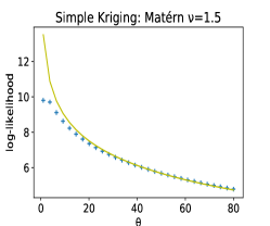
(a) Line: $-2\log(\theta)+13.5$

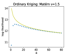
(b) Line: $-0.5\log(\theta)+14$

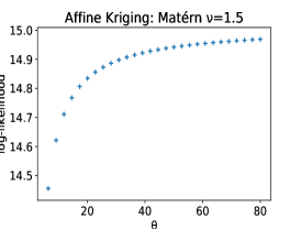
(c)

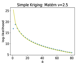
(d) Line: $-4.5\log(\theta)+25.5$

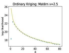
(e) Line: $-2\log(\theta)+25.7$

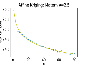
(f) Line: $-0.5\log(\theta)+25.95$

Figure 2: Logarithm of the likelihood function for large values of $\theta$ for varying Kriging models and correlation kernels. In each case, the design space is one-dimensional ($r=1$) and the design set is the 10-point regular grid on $[0,1]$. At every design point $x$, the observed value is $\sin(\pi x)$.

This behavior of the likelihood is a good reason to investigate the behavior of the tail rate of the reference prior density more closely than we did in Proposition 4.1.

All propositions in this appendix are valid under the assumption that some $n$-point design set has been fixed and that $n>p$.

Proposition B.1.

In the case of Affine Kriging, with a Matérn kernel with smoothness $\nu\in(1,2)$, the reference prior $\pi(\theta)$ is $O(\theta^{-2(2-\nu)-1})$ when $\theta\to+\infty$. It is a proper prior distribution. Furthermore, for every $\boldsymbol{y}\in\mathbb{R}^{n}$ such that $\boldsymbol{W}^{\top}\boldsymbol{y}$ is non-null, the likelihood function converges to a non-null constant when $\theta\to+\infty$.

Remark 7.

While this Proposition only provides an upper bound for the tail rate of the reference prior, the bound $O(\theta^{-2(2-\nu)-1})$ seems to be tight, judging by Figure 1c which was obtained with $\nu=3/2$.

Proof.

According to Lemma C.15, $\boldsymbol{\Sigma}_{\theta}$ can be written as:

$$\boldsymbol{\Sigma}_{\theta}=\boldsymbol{D}^{(0)}+\frac{a_{1}}{\theta^{2}}\boldsymbol{D}^{(1)}+\frac{a_{\nu}}{\theta^{2\nu}}\boldsymbol{D}^{(\nu)}+\frac{a_{2}}{\theta^{4}}\boldsymbol{D}^{(2)}+\boldsymbol{R}(\theta).$$ (B.1)

In the expression above,

• $a_{1}=-\Gamma(\nu-1)\nu/\Gamma(\nu)$,

• $a_{2}=\Gamma(\nu-2)\nu^{2}/\Gamma(\nu)$,

• $a_{\nu}=\Gamma(-\nu)\nu^{\nu}/\Gamma(\nu)$,

• $\boldsymbol{D}^{(0)}$ is the $n\times n$ matrix filled with ones,

• $\boldsymbol{D}^{(1)}$ is the $n\times n$ matrix with $(i,i^{\prime})$-th element $\left\|\boldsymbol{x}^{(i)}-\boldsymbol{x}^{(i^{\prime})}\right\|^{2}$,

• $\boldsymbol{D}^{(2)}$ is the $n\times n$ matrix with $(i,i^{\prime})$-th element $\left\|\boldsymbol{x}^{(i)}-\boldsymbol{x}^{(i^{\prime})}\right\|^{4}$,

• $\boldsymbol{D}^{(\nu)}$ is the $n\times n$ matrix with $(i,i^{\prime})$-th element $\left\|\boldsymbol{x}^{(i)}-\boldsymbol{x}^{(i^{\prime})}\right\|^{2\nu}$,

• $\boldsymbol{R}$ is a differentiable function from $(0,+\infty)$ to the space of real $n\times n$ matrices that satisfies $\|\boldsymbol{R}(\theta)\|=o(\theta^{-4})$ and $\|\frac{d}{d\theta}\boldsymbol{R}(\theta)\|=o(\theta^{-5})$ when $\theta\to+\infty$.

Under Affine Kriging, $\boldsymbol{H}$ is the $n\times(r+1)$ matrix whose first column is $\boldsymbol{1}$ (the vector of $\mathbb{R}^{n}$ filled with ones) and whose last $r$ columns contain the coordinates of the design set.

Because $\boldsymbol{W}$ is orthogonal to $\boldsymbol{H}$, Schoenberg (1937) (for example) implies that $\boldsymbol{W}^{\top}\boldsymbol{D}^{(0)}\boldsymbol{W}$ and $\boldsymbol{W}^{\top}\boldsymbol{D}^{(1)}\boldsymbol{W}$ are both null. We have therefore

$$\boldsymbol{W}^{\top}\boldsymbol{\Sigma}_{\theta}\boldsymbol{W}=\frac{a_{\nu}}{\theta^{2\nu}}\boldsymbol{W}^{\top}\boldsymbol{D}^{(\nu)}\boldsymbol{W}+\frac{a_{2}}{\theta^{4}}\boldsymbol{W}^{\top}\boldsymbol{D}^{(2)}\boldsymbol{W}+\boldsymbol{W}^{\top}\boldsymbol{R}(\theta)\boldsymbol{W}.$$ (B.2)

Using the notations from Appendix A.6, we can identify $\boldsymbol{Z}:=a_{\nu}\boldsymbol{D}^{(\nu)}$ and $\boldsymbol{Z}^{\star}:=a_{2}\boldsymbol{D}^{(2)}$. Thus $g(\theta):=\theta^{-2\nu}$ and $g(\theta)^{\star}:=\theta^{-2l}$ with $l=2-\nu$.

Besides, Lemma C.11 asserts that $\left\|\boldsymbol{\Sigma}_{\theta}^{-1}\right\|=O(\theta^{2\nu})$ when $\theta\to+\infty$. Applying Lemma C.1,

$$\boldsymbol{\Sigma}_{\theta}^{-1}=\boldsymbol{W}\left(\boldsymbol{W}^{\top}\boldsymbol{\Sigma}_{\theta}\boldsymbol{W}\right)^{-1}\boldsymbol{W}^{\top}+\boldsymbol{\Sigma}_{\theta}^{-1}\boldsymbol{H}\left(\boldsymbol{H}^{\top}\boldsymbol{\Sigma}_{\theta}^{-1}\boldsymbol{H}\right)^{-1}\boldsymbol{H}^{\top}\boldsymbol{\Sigma}_{\theta}^{-1}.$$ (B.3)

As both matrices in the right term are positive semi-definite, we have

$$\left\|\boldsymbol{W}\left(\boldsymbol{W}^{\top}\boldsymbol{\Sigma}_{\theta}\boldsymbol{W}\right)^{-1}\boldsymbol{W}^{\top}\right\|=O(\theta^{2\nu}).$$ (B.4)

And since $\boldsymbol{W}^{\top}\boldsymbol{W}=\boldsymbol{I}_{n-p}$, this implies that $\left\|\left(\boldsymbol{W}^{\top}\boldsymbol{\Sigma}_{\theta}\boldsymbol{W}\right)^{-1}\right\|=O(\theta^{2\nu})$.

Therefore $\boldsymbol{W}^{\top}\boldsymbol{D}^{(\nu)}\boldsymbol{W}$ is nonsingular. The proof of Theorem 4.4 given in Appendix A.6 yields the first assertion of this Proposition: the paragraph of Appendix A.6 below Equation (A.23) establishes in this situation that $\pi(\theta)=O(\theta^{-2l-1})=O(\theta^{-2(2-\nu)-1})$ and that the reference prior $\pi(\theta)$ is proper.

Moreover, given that $\boldsymbol{W}^{\top}\boldsymbol{D}^{(\nu)}\boldsymbol{W}$ is nonsingular, Equation (B.2) implies that, for every $\boldsymbol{y}\in\mathbb{R}^{n}$ such that $\boldsymbol{W}^{\top}\boldsymbol{y}$ is non-null,

$$\lim_{\theta\to+\infty}\left|\boldsymbol{W}^{\top}\boldsymbol{\Sigma}_{\theta}\boldsymbol{W}\right|^{-\frac{1}{2}}\left(\boldsymbol{y}^{\top}\boldsymbol{W}\right.\left(\boldsymbol{W}^{\top}\boldsymbol{\Sigma}_{\theta}\boldsymbol{W}\right)^{-1}\left.\boldsymbol{W}^{\top}\boldsymbol{y}\right)^{-\frac{n-p}{2}}$$

$$=\left|\boldsymbol{W}^{\top}\boldsymbol{D}^{(\nu)}\boldsymbol{W}\right|^{-\frac{1}{2}}\left(\boldsymbol{y}^{\top}\boldsymbol{W}\right.\left(\boldsymbol{W}^{\top}\boldsymbol{D}^{(\nu)}\boldsymbol{W}\right)^{-1}\left.\boldsymbol{W}^{\top}\boldsymbol{y}\right)^{-\frac{n-p}{2}}.$$ (B.5)

This implies that the likelihood function converges to a non-null constant. ∎

As mentioned in Appendix A.6, the case of Matérn kernels with integer smoothness is particularly tricky. Figure 3 focuses on the case where $\nu=1$. Once again, the most striking subfigure is the one showing the likelihood function under Affine Kriging: 3f. The behavior of the likelihood function and reference prior in this case is given in the following Proposition.

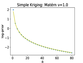
(a) $-\log(\theta)+1.8$

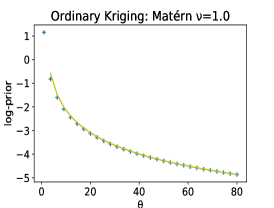
(b) $-\log(\theta)-\log(\log(\theta))+1$

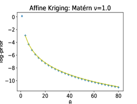
(c) $-3\log(\theta)+\log(\log(\theta))+0.7$

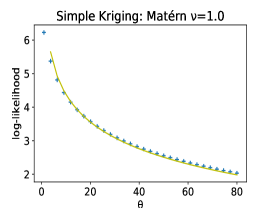
(d) $-\log(\theta)-\frac{1}{2}\log(\log(\theta))+7.1$

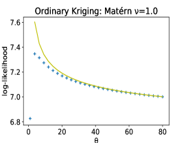
(e) $-\frac{1}{2}\log(\log(\theta))+7.74$

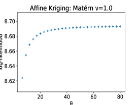
(f)

Figure 3: Logarithm of the prior (top) and likelihood function (bottom) for large values of $\theta$ for varying Kriging models using the Matérn kernel with smoothness $\nu=1$. In each case, the design space is one-dimensional ($r=1$) and the design set is the 10-point regular grid on $[0,1]$. At every design point $x$, the observed value is $\sin(\pi x)$.

Proposition B.2.

In the case of Affine Kriging, with a Matérn kernel with smoothness $\nu=1$, the reference prior $\pi(\theta)$ is $O(\theta^{-3}\log(\theta))$ when $\theta\to+\infty$. It is a proper prior distribution. Furthermore, for every $\boldsymbol{y}\in\mathbb{R}^{n}$ such that $\boldsymbol{W}^{\top}\boldsymbol{y}$ is non-null, the likelihood function converges to a non-null constant when $\theta\to+\infty$.

Remark 8.

While this Proposition is only able to provide an upper bound for the tail rate of the reference prior, the bound $O(\theta^{-3}\log(\theta))$ seems to be tight, judging by Figure 3c.

Proof.

We use Lemma C.17 to obtain:

$$\boldsymbol{\Sigma}_{\theta}=\boldsymbol{D}^{(0)}-2\left(\frac{\log(\theta)}{\theta^{2}}\boldsymbol{D}^{(1)}+\frac{1}{\theta^{2}}\boldsymbol{\tilde{D}}^{(1)}\right)+\frac{\log(\theta)}{\theta^{4}}\boldsymbol{D}^{(2)}+\boldsymbol{R}(\theta).$$ (B.6)

In the expression above,

• $\boldsymbol{D}^{(0)}$ is the $n\times n$ matrix filled with ones,

• $\boldsymbol{D}^{(1)}$ is the $n\times n$ matrix with $(i,i^{\prime})$-th element $\left\|\boldsymbol{x}^{(i)}-\boldsymbol{x}^{(i^{\prime})}\right\|^{2}$,

• $\boldsymbol{D}^{(2)}$ is the $n\times n$ matrix with $(i,i^{\prime})$-th element $\left\|\boldsymbol{x}^{(i)}-\boldsymbol{x}^{(i^{\prime})}\right\|^{4}$,

• $\boldsymbol{\tilde{D}}^{(1)}$ is the $n\times n$ matrix with null diagonal and $(i,i^{\prime})$-th element ($i\neq i^{\prime}$) given by

  $$\|\boldsymbol{x}^{(i)}-\boldsymbol{x}^{(i^{\prime})}\|^{2}\left\{-\log\left(\|\boldsymbol{x}^{(i)}-\boldsymbol{x}^{(i^{\prime})}\|\right)-\gamma+\frac{1}{2}\right\},$$

  where $\gamma$ is Euler’s constant,

• $\boldsymbol{R}$ is a differentiable function from $(0,+\infty)$ to the space of real $n\times n$ matrices that satisfies $\|\boldsymbol{R}(\theta)\|=O(\theta^{-4})$ and $\|\frac{d}{d\theta}\boldsymbol{R}(\theta)\|=O(\theta^{-5})$ when $\theta\to+\infty$.

The rest is similar to the proof of Proposition B.1. Using the notations of Appendix A.6, we have $\boldsymbol{Z}:=-2\boldsymbol{\tilde{D}}^{(1)}$, $\boldsymbol{Z}^{\star}:=\boldsymbol{D}^{(2)}$, $g(\theta):=\theta^{-2}$, $g^{\star}(\theta):=\theta^{-2l}\log(\theta)$ with $l=1$. The relevant part of Appendix A.6 is the part concerning Matérn kernels with integer smoothness: Appendix A.6.2. As $\nu=1$, we are in the case where either for all $\lambda\neq 0$, $\boldsymbol{Z}\neq\lambda\boldsymbol{D}^{(\nu)}$ or for all $\lambda^{\star}\neq 0$, $\boldsymbol{Z}^{\star}\neq\lambda^{\star}\boldsymbol{\tilde{D}}^{(\nu)}$. Here, both checks hold. Further, for the same reason as in the proof of Propostion B.1, we are in the subcase where $\boldsymbol{W}^{\top}\boldsymbol{Z}\boldsymbol{W}$ is nonsingular. In this subcase, Appendix A.6.2 states that the reference prior is $O(\theta^{-2l-1}\log(\theta))=O(\theta^{-3}\log(\theta))$ and that it is proper. Finally, $\boldsymbol{W}^{\top}\boldsymbol{Z}\boldsymbol{W}$ being nonsingular also leads to the conclusion that, for every $\boldsymbol{y}\in\mathbb{R}^{n}$ such that $\boldsymbol{W}^{\top}\boldsymbol{y}$ is non-null, the likelihood function converges to a non-null constant when $\theta$ goes to infinity. ∎

The most striking behavior of the reference prior density is given in Figure 3b (Ordinary Kriging), where the tail rate seems to be $\theta^{-1}\log(\theta)^{-1}$ multiplied by some constant factor. It decreases a little faster than the upper bound given in Proposition 4.1, $O(\theta^{-1})$, but still not fast enough to make the reference prior proper. Proposition B.3 below shows that $O(\theta^{-1}\log(\theta)^{-1})$ is indeed an upper bound for the reference prior.

Proposition B.3.

In the case of Ordinary Kriging, with a Matérn kernel with smoothness $\nu=1$, if $n>r+3$, then:

• the reference prior $\pi(\theta)$ is $O(\theta^{-1}\log(\theta)^{-1})$ when $\theta\to+\infty$;

• the matrix $\boldsymbol{W}^{\top}\boldsymbol{D}^{(1)}\boldsymbol{W}$ is singular;

• for every vector $\boldsymbol{y}\in\mathbb{R}^{n}$ such that $\boldsymbol{W}^{\top}\boldsymbol{y}$ does not belong to the vector subspace of $\mathbb{R}^{n-1}$ spanned by the columns of $\boldsymbol{W}^{\top}\boldsymbol{D}^{(1)}\boldsymbol{W}$, the reference posterior distribution $\pi(\theta|\boldsymbol{y})$ is $O(\theta^{-1}\log(\theta)^{-3/2})$ when $\theta\to+\infty$.

Remark 9.

The upper bound given for the reference posterior tail rate just barely makes it proper. Yet the tail rate suggested by Figure 3e for the likelihood function is consistent with it: $\log(\theta)^{-1/2}$ multiplied by some constant factor.

Proof.

The second assertion follows from Corollary 3.3. Only the first and third assertions need to be proved.

Let us use Lemma C.17 to obtain Equation (B.6).

With Ordinary Kriging, the matrix $\boldsymbol{H}$ is the vector $\boldsymbol{1}\in\mathbb{R}^{n}$ whose entries are all equal to 1. Therefore $\boldsymbol{W}^{\top}\boldsymbol{D}^{(0)}\boldsymbol{W}$ is the null $(n-1)\times(n-1)$ matrix and

$$\boldsymbol{W}^{\top}\boldsymbol{\Sigma}_{\theta}\boldsymbol{W}=-2\left(\frac{\log(\theta)}{\theta^{2}}\boldsymbol{W}\ ^{\top}\boldsymbol{D}^{(1)}\boldsymbol{W}+\frac{1}{\theta^{2}}\boldsymbol{W}^{\top}\boldsymbol{\tilde{D}}^{(1)}\boldsymbol{W}\right)$$ (B.7)

$$+\frac{\log(\theta)}{\theta^{4}}\boldsymbol{W}^{\top}\boldsymbol{D}^{(2)}\boldsymbol{W}+\boldsymbol{W}^{\top}\boldsymbol{R}(\theta)\boldsymbol{W}.$$

Using the notations of Appendix A.6, we have $\boldsymbol{Z}:=-2\boldsymbol{D}^{(1)}$ and $\boldsymbol{Z}^{\star}:=-2\boldsymbol{\tilde{D}}^{(1)}$, $g(\theta)=\theta^{-2}\log(\theta)$, $g^{\star}(\theta):=\log(\theta)^{-1}$.

Corollary 3.3 states that the rank of $\boldsymbol{Z}$ is lower or equal to $r+2$, so this is a fortiori true for the rank of $\boldsymbol{W}^{\top}\boldsymbol{Z}\boldsymbol{W}$. Since $r+2<n-1$, this implies that $\boldsymbol{W}^{\top}\boldsymbol{Z}\boldsymbol{W}$ is singular.

The proof of Theorem 4.4, Appendix A.6, then yields both results of this Proposition. The relevant part of Appendix A.6 is the part concerning Matérn kernels with integer smoothness: Appendix A.6.2. As $\nu=1$, we are in the case where there exists $\lambda\neq 0$ such that $\boldsymbol{Z}=\lambda\boldsymbol{D}^{(\nu)}$ ($\lambda=-2$) and there exists $\lambda^{\star}\neq 0$ such that $\boldsymbol{Z}^{\star}=\lambda^{\star}\boldsymbol{\tilde{D}}^{(\nu)}$ ($\lambda^{\star}=-2$). Further, we are in the subcase where $\boldsymbol{W}^{\top}\boldsymbol{Z}\boldsymbol{W}$ is singular. This subcase is dealt with in the last paragraph of Appendix A.6.2: it yields the first assertion.

Any vector $\boldsymbol{y}\in\mathbb{R}^{n}$ such that $\boldsymbol{W}^{\top}\boldsymbol{y}$ does not belong to the subspace of $\mathbb{R}^{n-1}$ spanned by the columns of $\boldsymbol{W}^{\top}\boldsymbol{D}^{(1)}\boldsymbol{W}$ verifies Assumption $\mathbb{\tilde{A}}_{1}(\boldsymbol{y})$ from Appendix A.7. Therefore Proposition A.4 can be applied instead of Proposition 4.3 and the last paragraph of Appendix A.6.2 yields the third assertion. ∎

Appendix C Auxiliary facts

Throughout this appendix, the following notations are used. We write $[\![\cdot,\cdot]\!]$ to denote intervals of integers. For example, $[\![1,3]\!]$ is the set $\{1,2,3\}$. We use the notation $\operatorname{Ker}$ to denote the kernel of a linear mapping or of a matrix. The “trivial vector space” is the vector space containing only the null vector.

C.1 Algebra

Lemma C.1.

Let $a$ and $b$ be positive integers and let $\boldsymbol{\Sigma}$ be a nonsingular symmetric $(a+b)\times(a+b)$ matrix. Then, for any $(a+b)\times a$ matrix $\boldsymbol{A}$ with rank $a$ and any $(a+b)\times b$ matrix $\boldsymbol{B}$ with rank $b$ such that $\boldsymbol{A}^{\top}\boldsymbol{B}$ is the null $a\times b$ matrix,

$$\boldsymbol{B}\left(\boldsymbol{B}^{\top}\boldsymbol{\Sigma}\boldsymbol{B}\right)^{-1}\boldsymbol{B}^{\top}=\boldsymbol{\Sigma}^{-1}\left(\boldsymbol{I}_{a+b}-\boldsymbol{A}\left(\boldsymbol{A}^{\top}\boldsymbol{\Sigma}^{-1}\boldsymbol{A}\right)^{-1}\boldsymbol{A}^{\top}\boldsymbol{\Sigma}^{-1}\right).$$ (C.1)

Lemma C.1 is used in the proofs of Propositions 2.1 and 2.2.

Proof.

This is a simple reformulation of Lemma 6 from Ren, Sun and He (2012). ∎

Lemma C.2.

Let $m$ be a positive integer, $\boldsymbol{\Sigma}$ be a nonsingular $m\times m$ matrix, and $\boldsymbol{A}$ and $\boldsymbol{B}$ be $m\times m$ matrices. If there exists a real number $t$ such that

$$\boldsymbol{A}=t\boldsymbol{\Sigma}+\boldsymbol{B},$$ (C.2)

then

$$\operatorname{Tr}\left[\left\{\boldsymbol{A}\boldsymbol{\Sigma}^{-1}\right\}^{2}\right]-\frac{1}{m}\left[\operatorname{Tr}\left\{\boldsymbol{A}\boldsymbol{\Sigma}^{-1}\right\}\right]^{2}=\operatorname{Tr}\left[\left\{\boldsymbol{B}\boldsymbol{\Sigma}^{-1}\right\}^{2}\right]-\frac{1}{m}\left[\operatorname{Tr}\left\{\boldsymbol{B}\boldsymbol{\Sigma}^{-1}\right\}\right]^{2}.$$ (C.3)

Lemma C.2 is used in the proof of Theorem 4.4.

Proof.

The lemma follows from a direct calculation:

$$\operatorname{Tr}\left[\boldsymbol{A}\boldsymbol{\Sigma}^{-1}\right] =\operatorname{Tr}\left[\boldsymbol{B}\boldsymbol{\Sigma}^{-1}\right]+tm.$$ (C.4)

$$\operatorname{Tr}\left[\left\{\boldsymbol{A}\boldsymbol{\Sigma}^{-1}\right\}^{2}\right] =\operatorname{Tr}\left[\left\{\boldsymbol{B}\boldsymbol{\Sigma}^{-1}\right\}^{2}\right]+2t\operatorname{Tr}\left[\boldsymbol{B}\boldsymbol{\Sigma}^{-1}\right]+t^{2}m.$$ (C.5)

∎

Lemma C.3.

Let $m>a$ be positive integers, $\boldsymbol{\Sigma}$ be an $m\times m$ symmetric positive definite matrix, $\boldsymbol{\Sigma}^{\prime}$ be an $m\times m$ symmetric matrix and $\boldsymbol{A}$ be an $m\times a$ matrix with rank $a$. Denote $\boldsymbol{Q}:=\boldsymbol{I}_{m}-\boldsymbol{A}\left(\boldsymbol{A}^{\top}\boldsymbol{\Sigma}^{-1}\boldsymbol{A}\right)^{-1}\boldsymbol{A}^{\top}\boldsymbol{\Sigma}^{-1}$. Then, if there exist $t_{1}\in\mathbb{R}$ and $t_{2}\in[0,+\infty)$ such that the matrix $\boldsymbol{F}:=t_{1}\boldsymbol{\Sigma}-\boldsymbol{\Sigma}^{\prime}$ is positive semi-definite and satisfies $\forall\boldsymbol{\xi}\in\mathbb{R}^{m}$ $\boldsymbol{\xi}^{\top}\boldsymbol{F}\boldsymbol{\xi}\leqslant t_{2}\boldsymbol{\xi}^{\top}\boldsymbol{\Sigma}\boldsymbol{\xi}$, then

$$\sqrt{\operatorname{Tr}\left[(\boldsymbol{\Sigma}^{\prime}\boldsymbol{\Sigma}^{-1}\boldsymbol{Q})^{2}\right]-\frac{1}{m-a}\left[\operatorname{Tr}\left\{\boldsymbol{\Sigma}^{\prime}\boldsymbol{\Sigma}^{-1}\boldsymbol{Q}\right\}\right]^{2}}\leqslant(m-a)t_{2}.$$ (C.6)

Moreover,

$$\sqrt{\operatorname{Tr}\left[(\boldsymbol{\Sigma}^{\prime}\boldsymbol{\Sigma}^{-1})^{2}\right]-\frac{1}{m}\left[\operatorname{Tr}\left\{\boldsymbol{\Sigma}^{\prime}\boldsymbol{\Sigma}^{-1}\right\}\right]^{2}}\leqslant mt_{2}.$$ (C.7)

Lemma C.3 is used in the proof of Proposition 4.1.

Proof.

Let $\boldsymbol{B}$ be an $m\times(m-a)$ matrix with rank $m-a$ such that $\boldsymbol{A}^{\top}\boldsymbol{B}$ is the null $a\times(m-a)$ matrix.

We only prove the first assertion. The proof of the second assertion is identical, except that $a$ must be replaced by 0 and $\boldsymbol{Q}$ and $\boldsymbol{B}$ must both be replaced by $\boldsymbol{I}_{m}$.

By applying Lemma C.1, we obtain that $\boldsymbol{\Sigma}^{-1}\boldsymbol{Q}=\boldsymbol{B}\left(\boldsymbol{B}^{\top}\boldsymbol{\Sigma}\boldsymbol{B}\right)^{-1}\boldsymbol{B}^{\top}$.

Because of the properties of the trace, this implies

$$\operatorname{Tr}\left[\boldsymbol{\Sigma}^{\prime}\boldsymbol{\Sigma}^{-1}\boldsymbol{Q}\right] =\operatorname{Tr}\left[\boldsymbol{B}^{\top}\boldsymbol{\Sigma}^{\prime}\boldsymbol{B}\left(\boldsymbol{B}^{\top}\boldsymbol{\Sigma}\boldsymbol{B}\right)^{-1}\right]$$ (C.8)

$$\operatorname{Tr}\left[(\boldsymbol{\Sigma}^{\prime}\boldsymbol{\Sigma}^{-1}\boldsymbol{Q})^{2}\right] =\operatorname{Tr}\left[\left\{\boldsymbol{B}^{\top}\boldsymbol{\Sigma}^{\prime}\boldsymbol{B}\left(\boldsymbol{B}^{\top}\boldsymbol{\Sigma}\boldsymbol{B}\right)^{-1}\right\}^{2}\right].$$ (C.9)

Similarly, we have

$$\operatorname{Tr}\left[\boldsymbol{F}\boldsymbol{\Sigma}^{-1}\boldsymbol{Q}\right] =\operatorname{Tr}\left[\boldsymbol{B}^{\top}\boldsymbol{F}\boldsymbol{B}\left(\boldsymbol{B}^{\top}\boldsymbol{\Sigma}\boldsymbol{B}\right)^{-1}\right]$$ (C.10)

$$\operatorname{Tr}\left[(\boldsymbol{F}\boldsymbol{\Sigma}^{-1}\boldsymbol{Q})^{2}\right] =\operatorname{Tr}\left[\left\{\boldsymbol{B}^{\top}\boldsymbol{F}\boldsymbol{B}\left(\boldsymbol{B}^{\top}\boldsymbol{\Sigma}\boldsymbol{B}\right)^{-1}\right\}^{2}\right].$$ (C.11)

Because $\boldsymbol{B}^{\top}\boldsymbol{F}\boldsymbol{B}=t_{1}\boldsymbol{B}^{\top}\boldsymbol{\Sigma}\boldsymbol{B}-\boldsymbol{B}^{\top}\boldsymbol{\Sigma}^{\prime}\boldsymbol{B}$, Lemma C.2 implies

$$\begin{split}&\operatorname{Tr}\left[\left\{\boldsymbol{B}^{\top}\boldsymbol{\Sigma}^{\prime}\boldsymbol{B}\left(\boldsymbol{B}^{\top}\boldsymbol{\Sigma}\boldsymbol{B}\right)^{-1}\right\}^{2}\right]-\frac{1}{m-a}\left[\operatorname{Tr}\left\{\boldsymbol{B}^{\top}\boldsymbol{\Sigma}^{\prime}\boldsymbol{B}\left(\boldsymbol{B}^{\top}\boldsymbol{\Sigma}\boldsymbol{B}\right)^{-1}\right\}\right]^{2}\\ =&\operatorname{Tr}\left[\left\{\boldsymbol{B}^{\top}\boldsymbol{F}\boldsymbol{B}\left(\boldsymbol{B}^{\top}\boldsymbol{\Sigma}\boldsymbol{B}\right)^{-1}\right\}^{2}\right]-\frac{1}{m-a}\left[\operatorname{Tr}\left\{\boldsymbol{B}^{\top}\boldsymbol{F}\boldsymbol{B}\left(\boldsymbol{B}^{\top}\boldsymbol{\Sigma}\boldsymbol{B}\right)^{-1}\right\}\right]^{2}.\end{split}$$ (C.12)

Combining the five equations above yields

$$\operatorname{Tr}\left[(\boldsymbol{\Sigma}^{\prime}\boldsymbol{\Sigma}^{-1}\boldsymbol{Q})^{2}\right]-\frac{1}{m-a}\left[\operatorname{Tr}\left\{\boldsymbol{\Sigma}^{\prime}\boldsymbol{\Sigma}^{-1}\boldsymbol{Q}\right\}\right]^{2}$$

$$= \operatorname{Tr}\left[\left(\boldsymbol{F}\boldsymbol{\Sigma}^{-1}\boldsymbol{Q}\right)^{2}\right]-\frac{1}{m-a}\left[\operatorname{Tr}\left\{\boldsymbol{F}\boldsymbol{\Sigma}^{-1}\boldsymbol{Q}\right\}\right]^{2}.$$ (C.13)

An elementary computation shows that $\boldsymbol{\Sigma}^{-1}\boldsymbol{Q}=\boldsymbol{Q}^{\top}\boldsymbol{\Sigma}^{-1}\boldsymbol{Q}$. Consider the Cholesky decomposition $\boldsymbol{\Sigma}=:\boldsymbol{L}\boldsymbol{L}^{\top}$. Then $\boldsymbol{\Sigma}^{-1}\boldsymbol{Q}=\boldsymbol{Q}^{\top}\boldsymbol{\Sigma}^{-1}\boldsymbol{Q}=\boldsymbol{Q}^{\top}\left(\boldsymbol{L}^{-1}\right)^{\top}\boldsymbol{L}^{-1}\boldsymbol{Q}$.

$$\operatorname{Tr}\left[\left(\boldsymbol{F}\boldsymbol{\Sigma}^{-1}\boldsymbol{Q}\right)^{2}\right] =\operatorname{Tr}\left[\left(\boldsymbol{F}\boldsymbol{Q}^{\top}\left(\boldsymbol{L}^{-1}\right)^{\top}\boldsymbol{L}^{-1}\boldsymbol{Q}\right)^{2}\right]=\operatorname{Tr}\left[\left(\boldsymbol{L}^{-1}\boldsymbol{Q}\boldsymbol{F}\boldsymbol{Q}^{\top}\left(\boldsymbol{L}^{-1}\right)^{\top}\right)^{2}\right]$$

$$\leqslant\left[\operatorname{Tr}\left\{\boldsymbol{L}^{-1}\boldsymbol{Q}\boldsymbol{F}\boldsymbol{Q}^{\top}\left(\boldsymbol{L}^{-1}\right)^{\top}\right\}\right]^{2}=\left[\operatorname{Tr}\left\{\boldsymbol{F}\boldsymbol{\Sigma}^{-1}\boldsymbol{Q}\right\}\right]^{2}.$$ (C.14)

The inequality holds because $\boldsymbol{L}^{-1}\boldsymbol{Q}\boldsymbol{F}\boldsymbol{Q}^{\top}\left(\boldsymbol{L}^{-1}\right)^{\top}$ is a symmetric positive semi-definite matrix.

Let $(\boldsymbol{\xi}_{i})_{1\leqslant i\leqslant m}$ be a basis of unit eigenvectors of $\boldsymbol{\Sigma}^{-1}\boldsymbol{Q}$ such that for every integer $i\in[\![1,m]\!]\setminus[\![1,m-a]\!]$, $\boldsymbol{\xi}_{i}$ belongs to the kernel of $\boldsymbol{\Sigma}^{-1}\boldsymbol{Q}$. Indeed, because $\boldsymbol{\Sigma}^{-1}\boldsymbol{Q}=\boldsymbol{B}\left(\boldsymbol{B}^{\top}\boldsymbol{\Sigma}\boldsymbol{B}\right)^{-1}\boldsymbol{B}^{\top}$, this kernel has the same dimension as the kernel of $\boldsymbol{B}^{\top}$: $a$.

Denoting by $(s_{i})_{1\leqslant i\leqslant m}$ the family of the eigenvalues corresponding to the family of eigenvectors $(\boldsymbol{\xi}_{i})_{1\leqslant i\leqslant m}$, we have for every integer $i\in[\![1,m-a]\!]$ $s_{i}\neq 0$ and

$$(\boldsymbol{\xi}_{i})^{\top}\boldsymbol{\Sigma}\boldsymbol{\xi}_{i} =s_{i}^{-2}\left\{(\boldsymbol{\xi}_{i})^{\top}\boldsymbol{Q}^{\top}\boldsymbol{\Sigma}^{-1}\right\}\boldsymbol{\Sigma}\left\{\boldsymbol{\Sigma}^{-1}\boldsymbol{Q}\boldsymbol{\xi}_{i}\right\}$$

$$=s_{i}^{-2}(\boldsymbol{\xi}_{i})^{\top}\boldsymbol{Q}^{\top}\boldsymbol{\Sigma}^{-1}\boldsymbol{Q}\boldsymbol{\xi}_{i}$$

$$=s_{i}^{-2}(\boldsymbol{\xi}_{i})^{\top}\boldsymbol{\Sigma}^{-1}\boldsymbol{Q}\boldsymbol{\xi}_{i}$$

$$=s_{i}^{-1}.$$ (C.15)

This implies the third equality below:

$$\operatorname{Tr}\left[\boldsymbol{F}\boldsymbol{\Sigma}^{-1}\boldsymbol{Q}\right] =\sum_{i=1}^{m}\left(\boldsymbol{\xi}_{i}\right)^{\top}\boldsymbol{F}\boldsymbol{\Sigma}^{-1}\boldsymbol{Q}\boldsymbol{\xi}_{i}$$

$$=\sum_{i=1}^{m-a}s_{i}\left(\boldsymbol{\xi}_{i}\right)^{\top}\boldsymbol{F}\boldsymbol{\xi}_{i}$$

$$=\sum_{i=1}^{m-a}\frac{\left(\boldsymbol{\xi}_{i}\right)^{\top}\boldsymbol{F}\boldsymbol{\xi}_{i}}{\left(\boldsymbol{\xi}_{i}\right)^{\top}\boldsymbol{\Sigma}\boldsymbol{\xi}_{i}}$$

$$\leqslant(m-a)t_{2}.$$ (C.16)

Equations (C.1) and (C.14) yield the result.

∎

Lemma C.4.

Let $(\boldsymbol{D}_{k})_{k\in\mathbb{N}}$ be a sequence of matrices of the same size. If $\sum_{k\in\mathbb{N}}\boldsymbol{D}_{k}$ exists and its kernel is the trivial vector space, then there exists a nonnegative integer $N$ such that $\cap_{k=0}^{N}\operatorname{Ker}\boldsymbol{D}_{k}$ is the trivial vector space.

Lemma C.4 is used in the proof of Lemma 4.2 and thus contributes to the proof of Theorem 4.4.

Proof.

Assume the sum $\sum_{k\in\mathbb{N}}\boldsymbol{D}_{k}$ exists and its kernel is the trivial vector space. Consider the sequence $(d(n))_{n\in\mathbb{N}}$ where for every nonnegative integer $n$, $d(n)$ is the dimension of $\cap_{k=0}^{n}\operatorname{Ker}\boldsymbol{D}^{(k)}$. $(d(n))_{n\in\mathbb{N}}$ is a nonincreasing sequence of nonegative integers, so it is convergent. If its limit is strictly greater than 0, then for every nonnegative integer $n$, there exists a unit vector $\boldsymbol{v}_{n}$ that belongs to $\cap_{k=0}^{n}\operatorname{Ker}\boldsymbol{D}^{(k)}$. Because the unit sphere is compact, there exists an increasing mapping $\phi:\mathbb{N}\to\mathbb{N}$ such that the subsequence $(\boldsymbol{v}_{\phi(n)})_{n\in\mathbb{N}}$ converges to a limit $\boldsymbol{v}$ such that $\|\boldsymbol{v}\|=1$. Besides, for every pair of nonnegative integers $n\leqslant n^{\prime}$, $\boldsymbol{v}_{\phi(n^{\prime})}\in\cap_{k=0}^{\phi(n)}\operatorname{Ker}\boldsymbol{D}^{(k)}$. Given this set is closed, the limit $\boldsymbol{v}$ also belongs to $\cap_{k=0}^{\phi(n)}\operatorname{Ker}\boldsymbol{D}^{(k)}$. So for every nonnegative integer $k$, $\boldsymbol{v}\in\operatorname{Ker}\boldsymbol{D}^{(k)}$ and therefore $\boldsymbol{v}\in\cap_{k=0}^{\infty}\operatorname{Ker}\boldsymbol{D}^{(k)}$. So $\boldsymbol{v}$ can only be the null vector, which is absurd since $\|\boldsymbol{v}\|=1$. We deduce from this contradiction that the limit of the sequence of integers $(d(n))_{n\in\mathbb{N}}$ is 0. Therefore there exists a nonnegative integer $N$ such that $d(N)=0$. ∎

C.2 Maclaurin series

The lemmas in this subsection deal with the following setting.

Let $m$ be a positive integer and let $\boldsymbol{M}$ be a continuous mapping from $\mathbb{R}$ to $\mathcal{M}_{m}$, the set of $m\times m$ matrices. Assume $\boldsymbol{M}$ admits the following Maclaurin series:

$$\boldsymbol{M}(t)=\sum_{k=0}^{N}a_{k}(t)\boldsymbol{A}_{k}+\boldsymbol{B}(t).$$ (C.17)

In the expression above, $N$ is a nonnegative integer and for every $k\in[\![0,N]\!]$:

1. $a_{k}$ is a continuous mapping $(0,+\infty)\to\mathbb{R}$ such that for all $t\in(0,+\infty)$, $a_{k}(t)\neq 0$;

2. for every nonnegative integer $l<k$, $a_{k}(t)=o(|a_{l}(t)|)$ when $t\to 0$;

3. $\boldsymbol{A}_{k}$ is a non-null symmetric $m\times m$ matrix.

$\boldsymbol{B}$ is a continuous mapping $(0,+\infty)\rightarrow\mathcal{M}_{m}$ such that for every $t\in\mathbb{R}$, $\boldsymbol{B}(t)$ is a symmetric matrix and when $t\to 0$, $\|\boldsymbol{B}(t)\|=o(|a_{N}(t)|)$.

Lemma C.5.

Consider (C.17). If $\cap_{k=0}^{N}\operatorname{Ker}\boldsymbol{A}_{k}$ is the trivial vector space and if there exists $T>0$ such that for all $t\in(0,T)$ $\boldsymbol{M}(t)$ is nonsingular, then when $t\to 0$, $\left\|\boldsymbol{M}(t)^{-1}\right\|=O\left(|a_{N}(t)|^{-1}\right)$.

Lemma C.5 and some elements of its proof below are used in the proof of Lemma C.6, which itself is used in the proof of Lemma 4.2 and thus contributes to the proof of Theorem 4.4. Lemma C.5 is also used in the proof of Lemma C.7, which is then used in the proof of Lemma C.19 and thus contributes to the proof of Proposition 4.1.

Proof.

Assume that $\cap_{k=0}^{N}\operatorname{Ker}\boldsymbol{A}_{k}$ is the trivial vector space and that there exists $T>0$ such that for all $t\in(0,T)$, $\boldsymbol{M}(t)$ is a nonsingular matrix.

If $N=0$, then $\boldsymbol{A}_{0}$ is nonsingular and the conclusion is trivial.

If $N\geqslant 1$, we may assume without loss of generality that $\cap_{k=0}^{N-1}\operatorname{Ker}\boldsymbol{A}_{k}$ is a nontrivial vector space, otherwise we could replace $N$ by $N-1$ and $\boldsymbol{B}(t)$ by $\left\{a_{N}(t)\boldsymbol{A}_{N}+\boldsymbol{B}(t)\right\}$ for all $t\in\mathbb{R}$.

Let $d_{N}$ be the dimension of the orthogonal complement of $\cap_{k=0}^{N-1}\operatorname{Ker}\boldsymbol{A}_{k}$. Let $\boldsymbol{W}_{N}$ be an $m\times(m-d_{N})$ matrix whose columns form an orthonormal basis of $\cap_{k=0}^{N-1}\operatorname{Ker}\boldsymbol{A}_{k}$, and let $\boldsymbol{P}_{N}$ be an $m\times d_{N}$ matrix whose columns form an orthonormal basis of its orthogonal complement. Then $(\boldsymbol{P}_{N},\boldsymbol{W}_{N})$ is an orthogonal matrix: it is the $m\times m$ matrix whose left $m\times d_{N}$ block is $\boldsymbol{P}_{N}$ and whose right $m\times(m-d_{N})$ block is $\boldsymbol{W}_{N}$. For all $t\in\mathbb{R}$, let us replace $\boldsymbol{M}(t)$ by $\tilde{\boldsymbol{M}}(t):=(\boldsymbol{P}_{N},\boldsymbol{W}_{N})^{\top}\boldsymbol{M}(t)(\boldsymbol{P}_{N},\boldsymbol{W}_{N})$. Because $(\boldsymbol{P}_{N},\boldsymbol{W}_{N})$ is an orthogonal matrix, the Frobenius norm of $\boldsymbol{M}(t)^{-1}$ is unchanged. Naturally, for all $k\in[\![0,N]\!]$, $\boldsymbol{A}_{k}$ is replaced by $\tilde{\boldsymbol{A}_{k}}:=(\boldsymbol{P}_{N},\boldsymbol{W}_{N})^{\top}\boldsymbol{A}_{k}(\boldsymbol{P}_{N},\boldsymbol{W}_{N})$ and for every $t\in\mathbb{R}$, $\boldsymbol{B}(t)$ is replaced by $\tilde{\boldsymbol{B}}(t):=(\boldsymbol{P}_{N},\boldsymbol{W}_{N})^{\top}\boldsymbol{B}(t)(\boldsymbol{P}_{N},\boldsymbol{W}_{N})$.

Now, for every $k\in[\![1,N]\!]$, $\tilde{\boldsymbol{A}}_{k}$ can be decomposed into blocks – a $d_{N}\times d_{N}$ block $\boldsymbol{A}_{k}^{\prime}$, an $(m-d_{N})\times(m-d_{N})$ block $\boldsymbol{A}_{k}^{\prime\prime}$ and a $d_{N}\times(m-d_{N})$ block $\boldsymbol{A}_{k}^{\prime\prime\prime}$:

$$\tilde{\boldsymbol{A}}_{k}=\begin{pmatrix}\boldsymbol{A}_{k}^{\prime}&\boldsymbol{A}_{k}^{\prime\prime\prime}\\ (\boldsymbol{A}_{k}^{\prime\prime\prime})^{\top}&\boldsymbol{A}_{k}^{\prime\prime}\end{pmatrix}.$$ (C.18)

For all $t\in(0,+\infty)$, $\boldsymbol{B}(t)$ can be decomposed in a similar manner (here the ^′ notation is used to distinguish the blocks, not to express some derivative with respect to $t$):

$$\tilde{\boldsymbol{B}}(t)=\begin{pmatrix}\boldsymbol{B}(t)^{\prime}&\boldsymbol{B}(t)^{\prime\prime\prime}\\ (\boldsymbol{B}(t)^{\prime\prime\prime})^{\top}&\boldsymbol{B}(t)^{\prime\prime}\end{pmatrix}.$$ (C.19)

Now, for any symmetric nonsingular matrix

$$\boldsymbol{C}=\begin{pmatrix}\boldsymbol{C}^{\prime}&\boldsymbol{C}^{\prime\prime\prime}\\ (\boldsymbol{C}^{\prime\prime\prime})^{\top}&\boldsymbol{C}^{\prime\prime}\end{pmatrix},$$ (C.20)

denoting by $\boldsymbol{S}:=\left\{\boldsymbol{C}^{\prime}-\boldsymbol{C}^{\prime\prime\prime}\left(\boldsymbol{C}^{\prime\prime}\right)^{-1}\left(\boldsymbol{C}^{\prime\prime\prime}\right)^{\top}\right\}$ the Schur complement of $\boldsymbol{C}^{\prime\prime}$, the inverse of $\boldsymbol{C}$ is

$$\boldsymbol{C}^{-1}=\begin{pmatrix}\boldsymbol{I}&\boldsymbol{0}\\ -\left(\boldsymbol{C}^{\prime\prime}\right)^{-1}\left(\boldsymbol{C}^{\prime\prime\prime}\right)^{\top}&\boldsymbol{I}\end{pmatrix}\begin{pmatrix}\boldsymbol{S}^{-1}&\boldsymbol{0}\\ \boldsymbol{0}&\left(\boldsymbol{C}^{\prime\prime}\right)^{-1}\end{pmatrix}\begin{pmatrix}\boldsymbol{I}&-\boldsymbol{C}^{\prime\prime\prime}\left(\boldsymbol{C}^{\prime\prime}\right)^{-1}\\ \boldsymbol{0}&\boldsymbol{I}\end{pmatrix}.$$ (C.21)

See the section about Block Factorization in Serre (2002) (p. 138-139) for explanations about how Equation (C.21) is obtained.

For every $k\in[\![0,N-1]\!]$, $\boldsymbol{A}_{k}^{\prime\prime}$ and $\boldsymbol{A}_{k}^{\prime\prime\prime}$ are null (note however that $\boldsymbol{A}_{N}^{\prime\prime}$ is nonsingular, otherwise $\cap_{k=0}^{N}\operatorname{Ker}\boldsymbol{A}_{k}$ would be nontrivial). For all $t\in(0,T)$, $\tilde{\boldsymbol{M}}(t)$ is nonsingular. Its lower $(m-d_{N})\times(m-d_{N})$ block is $\left\{a_{N}(t)\boldsymbol{A}_{N}^{\prime\prime}+\boldsymbol{B}(t)^{\prime\prime}\right\}$ and its Schur complement $\boldsymbol{S}_{N}(t)$ is

$$\begin{split}\boldsymbol{S}_{N}(t)&:=\left\{\sum_{k=0}^{N}a_{k}(t)\boldsymbol{A}_{k}^{\prime}+\boldsymbol{B}(t)^{\prime}\right\}-\\ &\left\{a_{N}(t)\boldsymbol{A}_{N}^{\prime\prime\prime}+\boldsymbol{B}(t)^{\prime\prime\prime}\right\}\left\{a_{N}(t)\boldsymbol{A}_{N}^{\prime\prime}+\boldsymbol{B}(t)^{\prime\prime}\right\}^{-1}\left\{a_{N}(t)\boldsymbol{A}_{N}^{\prime\prime\prime}+\boldsymbol{B}(t)^{\prime\prime\prime}\right\}^{\top}.\end{split}$$ (C.22)

Because we are dealing with the finite dimensional vector space of matrices of size $m\times m$, all norms are equivalent: for two norms $\|\cdot\|_{1}$ and $\|\cdot\|_{2}$, there exist positive constants $\kappa\leqslant\kappa^{\prime}$ such that for any matrix $\boldsymbol{X}$ of size $m\times m$,

$$\kappa\|\boldsymbol{X}\|_{1}\leqslant\|\boldsymbol{X}\|_{2}\leqslant\kappa^{\prime}\|\boldsymbol{X}\|_{1}.$$

In particular, the Frobenius norm is equivalent to the algebra norm

$$\boldsymbol{A}\mapsto\sup\left\{\sqrt{\boldsymbol{\xi}^{\top}\boldsymbol{A}^{\top}\boldsymbol{A}\boldsymbol{\xi}/\boldsymbol{\xi}^{\top}\boldsymbol{\xi}}\;:\;\boldsymbol{\xi}\in\mathbb{R}^{m}\setminus\{\boldsymbol{0}_{m}\}\right\}.$$

So there exists a constant $C_{m}\in(0,+\infty)$ such that for every $t\in(0,T)$,

$$\left\|\boldsymbol{M}(t)^{-1}\right\|\leqslant C_{m}\left(\|\boldsymbol{I}_{m}\|+\left\|\left\{a_{N}(t)\boldsymbol{A}_{N}^{\prime\prime\prime}+\boldsymbol{B}(t)^{\prime\prime\prime}\right\}\left\{a_{N}(t)\boldsymbol{A}_{N}^{\prime\prime}+\boldsymbol{B}(t)^{\prime\prime}\right\}^{-1}\right\|\right)^{2}$$

$$\left(\left\|\boldsymbol{S}_{N}(t)^{-1}\right\|+\left\|\left\{a_{N}(t)\boldsymbol{A}_{N}^{\prime\prime}+\boldsymbol{B}(t)^{\prime\prime}\right\}^{-1}\right\|\right).$$ (C.23)

$\boldsymbol{A}_{N}^{\prime\prime}$ is nonsingular, otherwise $\cap_{k=0}^{N}\operatorname{Ker}\boldsymbol{A}_{k}$ would be nontrivial. This means that the norm of the matrix $\left\{a_{N}(t)\boldsymbol{A}_{N}^{\prime\prime\prime}+\boldsymbol{B}(t)^{\prime\prime\prime}\right\}\left\{a_{N}(t)\boldsymbol{A}_{N}^{\prime\prime}+\boldsymbol{B}(t)^{\prime\prime}\right\}^{-1}$ is bounded when $t\to 0$. Because of Equation (C.2), this implies that there exists $T_{N}>0$ and $\lambda_{N}>0$ such that for all $t\in(0,T_{N})$,

$$\lambda_{N}\left\|\boldsymbol{M}(t)^{-1}\right\|\leqslant|a_{N}(t)|^{-1}+\left\|\boldsymbol{S}_{N}(t)^{-1}\right\|.$$ (C.24)

Our goal is to use Equation (C.24) recursively, by having $\boldsymbol{S}_{N}(t)$ play the part of $\boldsymbol{M}(t)$. To achieve this, a new expression of $\boldsymbol{S}_{N}(t)$ is required.

$$\boldsymbol{S}_{N}(t)=\sum_{k=0}^{N-1}a_{k}(t)\boldsymbol{A}_{k}^{\prime}+\boldsymbol{B}_{N}(t),$$ (C.25)

where

$$\begin{split}\boldsymbol{B}_{N}(t)&:=a_{N}(t)\boldsymbol{A}_{N}^{\prime}+\boldsymbol{B}(t)^{\prime}-\\ &\left\{a_{N}(t)\boldsymbol{A}_{N}^{\prime\prime\prime}+\boldsymbol{B}(t)^{\prime\prime\prime}\right\}\left\{a_{N}(t)\boldsymbol{A}_{N}^{\prime\prime}+\boldsymbol{B}(t)^{\prime\prime}\right\}^{-1}\left\{a_{N}(t)\boldsymbol{A}_{N}^{\prime\prime\prime}+\boldsymbol{B}(t)^{\prime\prime\prime}\right\}^{\top}.\end{split}$$ (C.26)

It turns out that when $t\to 0$, the norm of $\boldsymbol{B}_{N}(t)$ is $O(|a_{N}(t)|)$. This is due to the fact mentioned above that $\left\|\left\{a_{N}(t)\boldsymbol{A}_{N}^{\prime\prime\prime}+\boldsymbol{B}(t)^{\prime\prime\prime}\right\}\left\{a_{N}(t)\boldsymbol{A}_{N}^{\prime\prime}+\boldsymbol{B}(t)^{\prime\prime}\right\}^{-1}\right\|$ is bounded when $t\to 0$.

Furthermore, $\cap_{k=0}^{N-1}\operatorname{Ker}\boldsymbol{A}_{k}^{\prime}$ is the trivial vector space. Indeed, let $\boldsymbol{v}_{1}\in\cap_{k=0}^{N-1}\operatorname{Ker}\boldsymbol{A}_{k}^{\prime}$. Then for any vector $\boldsymbol{v}_{2}\in\mathbb{R}^{m-d_{N}}$, $(\boldsymbol{v}_{1},\boldsymbol{v}_{2})^{\top}\in\cap_{k=0}^{N-1}\operatorname{Ker}\tilde{\boldsymbol{A}}_{k}$. Independently from this, for any vector $\boldsymbol{v}_{3}\in\mathbb{R}^{d_{N}}$, $(\boldsymbol{v}_{3},\boldsymbol{0}_{m-d_{N}})^{\top}$ belongs to the orthogonal complement of $\cap_{k=0}^{N-1}\operatorname{Ker}\tilde{\boldsymbol{A}}_{k}$. So $(\boldsymbol{v}_{1},\boldsymbol{0}_{m-d_{N}})^{\top}$ belongs both to $\cap_{k=0}^{N-1}\operatorname{Ker}\tilde{\boldsymbol{A}}_{k}$ and its orthogonal complement: it is the null vector. Therefore $\boldsymbol{v}_{1}=\boldsymbol{0}_{d_{N}}$.

The two paragraphs above show that Equation (C.25) is formally similar to Equation (C.17): the role of $\boldsymbol{M}(t)$ is held by $\boldsymbol{S}_{N}(t)$, the role of $N$ by $N-1$, the role of the $\boldsymbol{A}_{k}$s by the $\boldsymbol{A}_{k}^{\prime}$s and the role of $\boldsymbol{B}(t)$ by $\boldsymbol{B}_{N}(t)$.

Therefore an equation similar to (C.24) can be derived: there exist $T_{N-1}>0$ and $\lambda_{N-1}>0$ such that for all $t\in(0,T_{N-1})$,

$$\lambda_{N-1}\left\|\boldsymbol{S}_{N}(t)^{-1}\right\|\leqslant|a_{N-1}(t)|^{-1}+\left\|\boldsymbol{S}_{N-1}(t)^{-1}\right\|.$$ (C.27)

Here, $\boldsymbol{S}_{N-1}(t)$ is defined with respect to $\boldsymbol{S}_{N}(t)$ the same way $\boldsymbol{S}_{N}(t)$ was defined with respect to $\boldsymbol{M}(t)$.

Recursive application of this reasoning until 0 is reached yields the result. ∎

Lemma C.6.

Consider (C.17). If $\cap_{k=0}^{N}\operatorname{Ker}\boldsymbol{A}_{k}$ is the trivial vector space, if the vector space $\cap_{k=0}^{N-1}\operatorname{Ker}\boldsymbol{A}_{k}$ is nontrivial, and if there exists $T>0$ such that for all $t\in(0,T)$, $\boldsymbol{M}(t)$ is positive definite, then for any vector $\boldsymbol{v}\in\mathbb{R}^{m}$ that does not belong to the vector space spanned by the columns of the matrices $\boldsymbol{A}_{k}$ ($1\leqslant k\leqslant N-1$),

$$\liminf_{t\to 0}\boldsymbol{v}\boldsymbol{M}(t)^{-1}\boldsymbol{v}/\left\|\boldsymbol{M}(t)^{-1}\right\|>0.$$ (C.28)

Lemma C.6 is used in the proof of Lemma 4.2 and thus contributes to the proof of Theorem 4.4.

Proof.

This result is trivial if $N=0$. If $N\geqslant 1$, it follows from the proof of Lemma C.5. Indeed, the requirements of this lemma are stronger than those of Lemma C.5, so all intermediate results of its proof are valid. Consider the right-hand side of Equation (C.21) while assuming $\boldsymbol{C}$ is positive definite. The matrices on the left-hand side and on the right-hand side are the transpose of one another, so the middle matrix is necessarily positive definite. In particular, both $\boldsymbol{S}^{-1}$ and $\left(\boldsymbol{C}^{\prime\prime}\right)^{-1}$ are positive definite. Any vector $\boldsymbol{v}\in\mathbb{R}^{m}$ can be decomposed as $\boldsymbol{v}=((\boldsymbol{v}^{\prime})^{\top},(\boldsymbol{v}^{\prime\prime})^{\top})^{\top}$ with $\boldsymbol{v}^{\prime}\in\mathbb{R}^{d_{N}}$ and $\boldsymbol{v}^{\prime\prime}\in\mathbb{R}^{m-d_{N}}$. This decomposition yields a lower bound: $\boldsymbol{v}^{\top}\boldsymbol{C}^{-1}\boldsymbol{v}\geqslant\left(\boldsymbol{v}^{\prime\prime}\right)^{\top}\left(\boldsymbol{C}^{\prime\prime}\right)^{-1}\boldsymbol{v}^{\prime\prime}$. Here, $\boldsymbol{C}$ is $\boldsymbol{M}(t)$, $\boldsymbol{S}$ is $\boldsymbol{S}_{N}(t)$ and $\boldsymbol{C}^{\prime\prime}$ is $a_{N}(t)\boldsymbol{A}_{N}^{\prime\prime}+\boldsymbol{B}^{\prime\prime}(t)$. Let us recall that $\boldsymbol{A}_{N}^{\prime\prime}$ is nonsingular and $\|\boldsymbol{B}^{\prime\prime}(t)\|=o(|a_{N}(t)|)$ when $t\to 0$. So as long as $\boldsymbol{v}$ is not orthogonal to $\cap_{k=0}^{N-1}\operatorname{Ker}\boldsymbol{A}_{k}$, $\boldsymbol{v}^{\prime\prime}$ is non-zero and there exists $\tilde{\lambda}_{N}(\boldsymbol{v})>0$ such that when $t$ is small enough, $\boldsymbol{v}^{\top}\boldsymbol{M}(t)^{-1}\boldsymbol{v}\geqslant\tilde{\lambda}_{N}(\boldsymbol{v})|a_{N}(t)|^{-1}$. Then Lemma C.5 yields the result.

∎

In order to be able to state the next lemmas, consider the vector spaces $V_{0},\dots,V_{N}$ recursively defined as follows:

$$V_{N}:=\cap_{k=0}^{N-1}\operatorname{Ker}\boldsymbol{A}_{k}.$$ (C.29)

For every positive integer $K$ smaller or equal to $N-1$:

$$V_{K}:=\left(\cap_{k=0}^{K-1}\operatorname{Ker}\boldsymbol{A}_{k}\right)\bigcap\left(\cap_{k=K+1}^{N}V_{k}^{\perp}\right).$$ (C.30)

Finally, define

$$V_{0}:=\cap_{k=1}^{N}V_{k}^{\perp}.$$ (C.31)

By construction, we have

$$\mathbb{R}^{m}=V_{0}\overset{\perp}{\oplus}V_{1}\overset{\perp}{\oplus}\dots\overset{\perp}{\oplus}V_{N}.$$ (C.32)

Lemma C.7.

Consider (C.17). Assume that $\cap_{k=0}^{N}\operatorname{Ker}\boldsymbol{A}_{k}$ is the trivial vector space. If there exists $T>0$ such that for all positive $t<T$, $\boldsymbol{M}(t)$ is positive definite, then for every nonnegative integer $k\leqslant N$, for all sufficiently small $t>0$, we have for every vector $\boldsymbol{\xi}_{k}\in V_{k}\setminus\{\boldsymbol{0}\}$ $a_{k}(t)\boldsymbol{\xi}_{k}^{\top}\boldsymbol{A}_{k}\boldsymbol{\xi}_{k}>0$.

Lemma C.7 gives a sufficient condition for one of the assumptions of Lemma C.8 below. Lemma C.8 is used in the proof of Lemma C.19 and thus contributes to the proof of Proposition 4.1.

Remark 10.

Note that for any nonnegative integer $k\leqslant N$, the assertion “for all sufficiently small $t>0$, we have for every vector $\boldsymbol{\xi}_{k}\in V_{k}\setminus\{\boldsymbol{0}\}$ $a_{k}(t)\boldsymbol{\xi}_{k}^{\top}\boldsymbol{A}_{k}\boldsymbol{\xi}_{k}>0$” implies that one of the following assertions is true:

• For all $\boldsymbol{\xi}_{k}\in V_{k}\setminus\{\boldsymbol{0}\}$, $\boldsymbol{\xi}_{k}^{\top}\boldsymbol{A}_{k}\boldsymbol{\xi}_{k}>0$.

• For all $\boldsymbol{\xi}_{k}\in V_{k}\setminus\{\boldsymbol{0}\}$, $\boldsymbol{\xi}_{k}^{\top}\boldsymbol{A}_{k}\boldsymbol{\xi}_{k}<0$.

Proof.

Assume that $\cap_{k=0}^{N}\operatorname{Ker}\boldsymbol{A}_{k}$ is the trivial vector space and that there exists $T>0$ such that for all positive $t<T$, $\boldsymbol{M}(t)$ is positive definite.

If the conclusion of Lemma C.7 does not hold, then there exist a nonnegative integer $K\leqslant N$, a sequence $(t_{l})_{l\in\mathbb{N}}$ of non-null real numbers converging to 0 and a sequence $(\boldsymbol{\xi}_{K,l})_{l\in\mathbb{N}}$ of vectors of $V_{K}$ satisfying $\boldsymbol{\xi}_{K,l}^{\top}\boldsymbol{\xi}_{K,l}=1$ such that $a_{K}(t_{l})\boldsymbol{\xi}_{K,l}^{\top}\boldsymbol{A}_{K}\boldsymbol{\xi}_{K,l}\leqslant 0$ for all $l\in\mathbb{N}$.

Let $\boldsymbol{W}_{K}$ be a matrix with $m$ rows and with number of columns equal to the dimension of $V_{0}+\dots+V_{K}$ such that for any vector $\boldsymbol{\xi}\in V_{0}+\dots+V_{K}$, $\boldsymbol{W}_{K}\boldsymbol{W}_{K}^{\top}\boldsymbol{\xi}=\boldsymbol{\xi}$. For any sufficiently great $l\in\mathbb{N}$, $\boldsymbol{M}(t_{l})$ is positive definite. Given that the kernel of $\boldsymbol{W}_{K}$ is the trivial vector space, $\boldsymbol{W}_{K}^{\top}\boldsymbol{M}(t_{l})\boldsymbol{W}_{K}$ is positive definite as well. Moreover, $\cap_{k=0}^{K}\operatorname{Ker}\boldsymbol{W}_{K}^{\top}\boldsymbol{A}_{k}\boldsymbol{W}_{K}$ is the trivial vector space. This means that Lemma C.5 is applicable and $\left\|\left(\boldsymbol{W}_{K}\boldsymbol{M}(t_{l})\boldsymbol{W}_{K}\right)^{-1}\right\|=O(|a_{K}(t_{l})|^{-1})$ when $l\to+\infty$.

However, for all $l\in\mathbb{N}$,

$$a_{K}(t_{l})\boldsymbol{\xi}_{K,l}^{\top}\boldsymbol{A}_{K}\boldsymbol{\xi}_{K,l}=a_{K}(t_{l})\boldsymbol{\xi}_{K,l}^{\top}\boldsymbol{W}_{K}\left(\boldsymbol{W}_{K}^{\top}\boldsymbol{A}_{K}\boldsymbol{W}_{K}\right)\boldsymbol{W}_{K}^{\top}\boldsymbol{\xi}_{K,l}\leqslant 0.$$ (C.33)

Since for every nonnegative integer $k<K$ and every nonnegative integer $l$, $\boldsymbol{\xi}_{K,l}^{\top}\boldsymbol{W}_{K}\left(\boldsymbol{W}_{K}^{\top}\boldsymbol{A}_{k}\boldsymbol{W}_{K}\right)\boldsymbol{W}_{K}^{\top}\boldsymbol{\xi}_{K,l}=0$, this implies that when $l\to+\infty$,

$$a_{K}(t_{l})\boldsymbol{\xi}_{K,l}^{\top}\boldsymbol{W}_{K}\left(\boldsymbol{W}_{K}^{\top}\boldsymbol{M}(t_{l})\boldsymbol{W}_{K}\right)\boldsymbol{W}_{K}^{\top}\boldsymbol{\xi}_{K,l}=o(|a_{K}(t_{l})|).$$ (C.34)

This contradicts the earlier result that when $l\to+\infty$,

$$\left\|\left(\boldsymbol{W}_{K}\boldsymbol{M}(t_{l})\boldsymbol{W}_{K}\right)^{-1}\right\|=O(|a_{K}(t_{l})|^{-1}).$$ (C.35)

Therefore the conclusion of Lemma C.7 must hold. ∎

Lemma C.8.

Consider (C.17). Assume that $\cap_{k=0}^{N}\operatorname{Ker}\boldsymbol{A}_{k}$ is the trivial vector space. Further assume that for any nonnegative integer $k\leqslant N$, for all sufficiently small $t>0$ and for all $\tilde{\boldsymbol{\xi}}_{k}\in V_{k}\setminus\{\boldsymbol{0}\}$, $a_{k}(t)\tilde{\boldsymbol{\xi}}_{k}^{\top}\boldsymbol{A}_{k}\tilde{\boldsymbol{\xi}}_{k}>0$. Then, for any $\epsilon>0$, there exists a real number $T>0$ such that for all $t\in(0,T)$ and for any vector $\boldsymbol{\xi}\in\mathbb{R}^{m}$, letting $\boldsymbol{\xi}=\boldsymbol{\xi}_{0}+\dots+\boldsymbol{\xi}_{N}$ be its unique decomposition according to the subspaces $V_{0},\dots,V_{N}$,

$$(1-\epsilon)\sum_{k=0}^{N}a_{k}(t)\boldsymbol{\xi}_{k}^{\top}\boldsymbol{A}_{k}\boldsymbol{\xi}_{k}\leqslant\boldsymbol{\xi}^{\top}\boldsymbol{M}(t)\boldsymbol{\xi}\leqslant(1+\epsilon)\sum_{k=0}^{N}a_{k}(t)\boldsymbol{\xi}_{k}^{\top}\boldsymbol{A}_{k}\boldsymbol{\xi}_{k}.$$ (C.36)

Lemma C.8 is used in the proof of Lemma C.19 and thus contributes to the proof of Proposition 4.1.

Proof.

For any nonnegative integers $k$, $m$ and $m^{\prime}$ that are smaller or equal to $N$, if either $m>k$ or $m^{\prime}>k$, then

$$\boldsymbol{\xi}_{m}^{\top}\boldsymbol{A}_{k}\boldsymbol{\xi}_{m^{\prime}}=0.$$ (C.37)

This means that

$$\boldsymbol{\xi}^{\top}\boldsymbol{M}(t)\boldsymbol{\xi} =\underbrace{\sum_{k=0}^{N}a_{k}(t)\boldsymbol{\xi}_{k}^{\top}\boldsymbol{A}_{k}\boldsymbol{\xi}_{k}}_{f_{1}(t)}+$$

$$\quad\underbrace{\sum_{k=0}^{N}\left(\sum_{\begin{subarray}{c}0\leqslant m,m^{\prime}\leqslant k\leqslant N\\ m\neq k\,\mathrm{or}\,m^{\prime}\neq k\end{subarray}}a_{k}(t)\boldsymbol{\xi}_{m}^{\top}\boldsymbol{A}_{k}\boldsymbol{\xi}_{m^{\prime}}\right)}_{f_{2}(t)}+\underbrace{\sum_{0\leqslant m,m^{\prime}\leqslant N}\boldsymbol{\xi}_{m}^{\top}\boldsymbol{B}(t)\boldsymbol{\xi}_{m^{\prime}}}_{f_{3}(t)}.$$ (C.38)

Let us examine every term in $f_{2}(t)$ and $f_{3}(t)$.

To do this, define

$$d_{k}^{min}:=\min\{|\boldsymbol{\xi}_{k}^{\top}\boldsymbol{A}_{k}\boldsymbol{\xi}_{k}|:\boldsymbol{\xi}_{k}\in V_{k},\boldsymbol{\xi}_{k}^{\top}\boldsymbol{\xi}_{k}=1\}.$$

And then

$$d^{min}:=\min\{d_{k}^{min}:k\in\mathbb{N},0\leqslant k\leqslant N\}.$$

Due to the assumption that for any integer $k\in[\![0,N]\!]$, for all sufficiently small $t>0$, $a_{k}(t)\boldsymbol{\xi}_{k}^{\top}\boldsymbol{A}_{k}\boldsymbol{\xi}_{k}>0$,

$$d^{min}>0.$$ (C.39)

For good measure, also define

$$d^{max}:=\max\{\|\boldsymbol{A}_{k}\|:k\in\mathbb{N},0\leqslant k\leqslant N\}.$$

Choose a real number $\epsilon>0$.

For any nonnegative intergers $m,m^{\prime}\leqslant N$,

$$|\boldsymbol{\xi}_{m}^{\top}\boldsymbol{B}(t)\boldsymbol{\xi}_{m^{\prime}}|\leqslant\|\boldsymbol{B}(t)\|\|\boldsymbol{\xi}_{m}\|\|\boldsymbol{\xi}_{m^{\prime}}\|\leqslant\|\boldsymbol{B}(t)\|(\boldsymbol{\xi}_{m}^{\top}\boldsymbol{\xi}_{m}+\boldsymbol{\xi}_{m^{\prime}}^{\top}\boldsymbol{\xi}_{m^{\prime}}).$$ (C.40)

Because $\|\boldsymbol{B}(t)\|=o(|a_{N}(t)|)$, there exists $T_{B}>0$ such that for all $t\in(0,T_{B})$ and for any nonnegative integer $K\leqslant N$:

$$\|\boldsymbol{B}(t)\|\leqslant|a_{K}(t)|d^{min}\epsilon.$$ (C.41)

It follows that for all $t\in(0,T_{B})$:

$$\|\boldsymbol{B}(t)\|(\boldsymbol{\xi}_{m}^{\top}\boldsymbol{\xi}_{m}+\boldsymbol{\xi}_{m^{\prime}}^{\top}\boldsymbol{\xi}_{m^{\prime}})\leqslant\epsilon\left(a_{m}(t)\boldsymbol{\xi}_{m}^{\top}\boldsymbol{A}_{m}\boldsymbol{\xi}_{m}+a_{m^{\prime}}(t)\boldsymbol{\xi}_{m^{\prime}}^{\top}\boldsymbol{A}_{m^{\prime}}\boldsymbol{\xi}_{m^{\prime}}\right).$$ (C.42)

Therefore, for all $t\in(0,T_{B})$:

$$|\boldsymbol{\xi}_{m}^{\top}\boldsymbol{B}(t)\boldsymbol{\xi}_{m^{\prime}}|\leqslant\epsilon\left(a_{m}(t)\boldsymbol{\xi}_{m}^{\top}\boldsymbol{A}_{m}\boldsymbol{\xi}_{m}+a_{m^{\prime}}(t)\boldsymbol{\xi}_{m^{\prime}}^{\top}\boldsymbol{A}_{m^{\prime}}\boldsymbol{\xi}_{m^{\prime}}\right).$$ (C.43)

And then, for all $t\in(0,T_{B})$:

$$|f_{3}(t)|\leqslant\epsilon\sum_{0\leqslant m,m^{\prime}\leqslant N}a_{m}(t)\boldsymbol{\xi}_{m}^{\top}\boldsymbol{A}_{m}\boldsymbol{\xi}_{m}+a_{m^{\prime}}(t)\boldsymbol{\xi}_{m^{\prime}}^{\top}\boldsymbol{A}_{m^{\prime}}\boldsymbol{\xi}_{m^{\prime}}=\epsilon 2(N+1)f_{1}(t).$$ (C.44)

For any nonegative integers $m,m^{\prime},k\leqslant N$ such that both $m\leqslant k$ and $m^{\prime}\leqslant k$:

$$|\boldsymbol{\xi}_{m}^{\top}\boldsymbol{A}_{k}\boldsymbol{\xi}_{m^{\prime}}|\leqslant\|\boldsymbol{A}_{k}\|\|\boldsymbol{\xi}_{m}\|\|\boldsymbol{\xi}_{m^{\prime}}\|\leqslant d^{max}(\boldsymbol{\xi}_{m}^{\top}\boldsymbol{\xi}_{m}+\boldsymbol{\xi}_{m^{\prime}}^{\top}\boldsymbol{\xi}_{m^{\prime}}).$$ (C.45)

Let us first consider the case where both $m<k$ and $m^{\prime}<k$. Then, since $|a_{k}(t)|=o(|a_{m}(t)|)$ and $|a_{k}(t)|=o(|a_{m^{\prime}}(t)|)$, there exists $T_{m,m^{\prime},k}>0$ such that for all $t\in(0,T_{m,m^{\prime},k})$,

$$d^{max}|a_{k}(t)|\leqslant d^{min}\min(|a_{m}(t)|,|a_{m^{\prime}}(t)|)\epsilon.$$ (C.46)

So, in the case where both $m<k$ and $m^{\prime}<k$, we have for all $t\in(0,T_{m,m^{\prime},k})$:

$$|\boldsymbol{\xi}_{m}^{\top}\boldsymbol{A}_{k}\boldsymbol{\xi}_{m^{\prime}}|\leqslant\epsilon\left(a_{m}(t)\boldsymbol{\xi}_{m}^{\top}\boldsymbol{A}_{m}\boldsymbol{\xi}_{m}+a_{m^{\prime}}(t)\boldsymbol{\xi}_{m^{\prime}}^{\top}\boldsymbol{A}_{m^{\prime}}\boldsymbol{\xi}_{m^{\prime}}\right).$$ (C.47)

Let us now consider the case where $m<k$ and $m^{\prime}=k$ (the case where $m=k$ and $m^{\prime}<k$ being equivalent since $\boldsymbol{A}_{k}$ is symmetric).

$$|\boldsymbol{\xi}_{m}^{\top}\boldsymbol{A}_{k}\boldsymbol{\xi}_{k}|\leqslant\|\boldsymbol{A}_{k}\|\|\boldsymbol{\xi}_{m}\|\|\boldsymbol{\xi}_{k}\|\leqslant d^{max}\|\boldsymbol{\xi}_{m}\|\|\boldsymbol{\xi}_{k}\|.$$ (C.48)

If $\|\boldsymbol{\xi}_{m}\|\leqslant\epsilon(d^{min}/d^{max})\|\boldsymbol{\xi}_{k}\|$, then:

$$|\boldsymbol{\xi}_{m}^{\top}\boldsymbol{A}_{k}\boldsymbol{\xi}_{k}|\leqslant d^{min}\boldsymbol{\xi}_{k}^{\top}\boldsymbol{\xi}_{k}\epsilon\leqslant\boldsymbol{\xi}_{k}^{\top}\boldsymbol{A}_{k}\boldsymbol{\xi}_{k}\epsilon.$$ (C.49)

If $\|\boldsymbol{\xi}_{m}\|>\epsilon(d^{min}/d^{max})\|\boldsymbol{\xi}_{k}\|$, then:

$$|\boldsymbol{\xi}_{m}^{\top}\boldsymbol{A}_{k}\boldsymbol{\xi}_{k}|<\frac{d^{max}}{\epsilon(d^{min}/d^{max})}\boldsymbol{\xi}_{m}^{\top}\boldsymbol{\xi}_{m}.$$ (C.50)

Since $|a_{k}(t)|=o(|a_{m}(t)|)$, there exists $T_{m,k}>0$ such that for all $t\in(0,T_{m,k})$,

$$\frac{d^{max}}{\epsilon(d^{min}/d^{max})}|a_{k}(t)|\leqslant d^{min}|a_{m}(t)|\epsilon.$$ (C.51)

Therefore, if $\|\boldsymbol{\xi}_{m}\|>\epsilon(d^{min}/d^{max})\|\boldsymbol{\xi}_{k}\|$, provided $t\in(0,T_{m,k})$,

$$|a_{k}(t)||\boldsymbol{\xi}_{m}^{\top}\boldsymbol{A}_{k}\boldsymbol{\xi}_{k}|<a_{m}(t)d^{min}\boldsymbol{\xi}_{m}^{\top}\boldsymbol{\xi}_{m}\epsilon\leqslant a_{m}(t)\boldsymbol{\xi}_{m}^{\top}\boldsymbol{A}_{m}\boldsymbol{\xi}_{m}\epsilon.$$ (C.52)

Putting together (C.49) and (C.52), we obtain that for all $\boldsymbol{\xi}\in\mathbb{R}^{m}$, for all $t\in(0,T_{m,k})$,

$$|\boldsymbol{\xi}_{m}^{\top}\boldsymbol{A}_{k}\boldsymbol{\xi}_{k}|\leqslant\epsilon\left(a_{m}(t)\boldsymbol{\xi}_{m}^{\top}\boldsymbol{A}_{m}\boldsymbol{\xi}_{m}+a_{k}(t)\boldsymbol{\xi}_{k}^{\top}\boldsymbol{A}_{k}\boldsymbol{\xi}_{k}\right).$$ (C.53)

Define

$$T_{A}:=\min( \min\{T_{m,m^{\prime},k}|m,m^{\prime},k\in\mathbb{N};0\leqslant m,m^{\prime}<k\leqslant N\},$$

$$\min\{T_{m,k}|m,k\in\mathbb{N};0\leqslant m<k\leqslant N\}).$$

For all $t\in(0,T_{A})$,

$$|f_{2}(t)| \leqslant\epsilon\sum_{k=0}^{N}\left(\sum_{\begin{subarray}{c}0\leqslant m,m^{\prime}\leqslant k\leqslant N\\ m\neq k\,\mathrm{or}\,m^{\prime}\neq k\end{subarray}}\left(a_{m}(t)\boldsymbol{\xi}_{m}^{\top}\boldsymbol{A}_{m}\boldsymbol{\xi}_{m}+a_{m^{\prime}}(t)\boldsymbol{\xi}_{m^{\prime}}^{\top}\boldsymbol{A}_{m^{\prime}}\boldsymbol{\xi}_{m^{\prime}}\right)\right)$$

$$\leqslant\epsilon(N+1)\sum_{0\leqslant m,m^{\prime}\leqslant N}\left(a_{m}(t)\boldsymbol{\xi}_{m}^{\top}\boldsymbol{A}_{m}\boldsymbol{\xi}_{m}+a_{m^{\prime}}(t)\boldsymbol{\xi}_{m^{\prime}}^{\top}\boldsymbol{A}_{m^{\prime}}\boldsymbol{\xi}_{m^{\prime}}\right)$$

$$\leqslant\epsilon 2(N+1)^{2}f_{1}(t).$$ (C.54)

Defining $T:=\min(T_{A},T_{B})$, Equations (C.44) and (C.54) yield that for all $t\in(0,T)$,

$$|f_{2}(t)|+|f_{3}(t)|\leqslant\epsilon 2(N+2)^{2}f_{1}(t).$$ (C.55)

As $\epsilon$ can be taken arbitrarily small, after redefining $\epsilon:=\epsilon/(2(N+2)^{2})$, this yields the result. ∎

C.3 Bound for $\left\|\boldsymbol{\Sigma}_{\theta}^{-1}\right\|$ with Matérn kernels

In order to derive a bound for $\left\|\boldsymbol{\Sigma}_{\theta}^{-1}\right\|$ in the case of Matérn kernels (Lemma C.11), the spectral representation of the kernels is convenient.

To use it, we need this preliminary Bochner-type result:

Lemma C.9.

Let $\mu$ be a positive measure on $\mathbb{R}^{r}$ with finite non-null total mass that is absolutely continuous with respect to the Lebesgue measure. Then the mapping $K:\mathbb{R}^{r}\rightarrow\mathbb{R}$ defined by

$$K(\boldsymbol{x})=\int_{\mathbb{R}^{r}}e^{i\langle\boldsymbol{\omega}|\boldsymbol{x}\rangle}d\mu(\boldsymbol{\omega})$$ (C.56)

is positive definite. Moreover, for any $\boldsymbol{\xi}\in\mathbb{R}^{n}\setminus\{\boldsymbol{0}_{n}\}$,

$$\sum_{k,l\in[\![1,n]\!]}\xi_{k}\xi_{l}K(\boldsymbol{x}^{(k)}-\boldsymbol{x}^{(l)})>0.$$ (C.57)

Proof.

The first part results from Bochner’s theorem. Let us show the second.

$$\sum_{k,l\in[\![1,n]\!]}\xi_{k}\xi_{l}K(\boldsymbol{x}^{(k)}-\boldsymbol{x}^{(l)}) =\sum_{k,l\in[\![1,n]\!]}\xi_{k}\xi_{l}\int_{\mathbb{R}^{r}}e^{i\langle\boldsymbol{\omega}|\boldsymbol{x}^{(k)}-\boldsymbol{x}^{(l)}\rangle}d\mu(\boldsymbol{\omega})$$

$$=\int_{\mathbb{R}^{r}}\left|\sum_{k=1}^{n}\xi_{k}e^{i\langle\boldsymbol{\omega}|\boldsymbol{x}^{(k)}\rangle}\right|^{2}d\mu(\boldsymbol{\omega}).$$ (C.58)

Given $\boldsymbol{x}^{(1)},...,\boldsymbol{x}^{(n)}$ are all distinct, for almost all unitary vectors $\boldsymbol{u}$ in the sense of the Lebesgue measure on the unit sphere $S^{r-1}$, the real numbers $\langle\boldsymbol{u}|\boldsymbol{x}^{(1)}\rangle,...,\langle\boldsymbol{u}|\boldsymbol{x}^{(n)}\rangle$ are distinct. Indeed, if two of these numbers, say $\langle\boldsymbol{u}|\boldsymbol{x}^{(1)}\rangle$ and $\langle\boldsymbol{u}|\boldsymbol{x}^{(2)}\rangle$, were equal, then $\boldsymbol{u}$ would be orthogonal to $\boldsymbol{x}^{(1)}-\boldsymbol{x}^{(2)}$. But the set of all vectors of $\mathbb{R}^{r}$ orthogonal to $\boldsymbol{x}^{(1)}-\boldsymbol{x}^{(2)}$ is a hyperplane. So there exists a finite number of hyperplanes of $\mathbb{R}^{r}$ such that, if $\boldsymbol{u}$ does not belong to any of them, the real numbers $\langle\boldsymbol{u}|\boldsymbol{x}^{(1)}\rangle,...,\langle\boldsymbol{u}|\boldsymbol{x}^{(n)}\rangle$ are distinct.

Now, notice that the mapping $\mathbb{C}\rightarrow\mathbb{C};z\mapsto\sum_{k=1}^{n}\xi_{k}e^{iz\langle\boldsymbol{u}|\boldsymbol{x}^{(k)}\rangle}$ is holomorphic. So either it is the null function or all its zeros are isolated. Given it clearly is not the null function, its zeros are isolated. So the set of all zeros that belong to $\mathbb{R}$ is countable and therefore of null Lebesgue measure.

Let $f:\mathbb{R}^{r}\rightarrow\{0,1\}$ be the measurable mapping such that $f(\boldsymbol{\omega})=1$ if $\sum_{k=1}^{n}\xi_{k}e^{i\langle\boldsymbol{\omega}|\boldsymbol{x}^{(k)}\rangle}=0$ and $f(\boldsymbol{\omega})=0$ if not.

$$\int_{\mathbb{R}^{r}}f(\boldsymbol{\omega})d\boldsymbol{\omega}=\frac{2\pi^{\frac{r}{2}}}{\Gamma\left(\frac{r}{2}\right)}\int_{S^{r-1}}\int_{(0,+\infty)}f(t\boldsymbol{u})t^{r-1}dtd\boldsymbol{u}=\frac{2\pi^{\frac{r}{2}}}{\Gamma\left(\frac{r}{2}\right)}\int_{S^{r-1}}0\,d\boldsymbol{u}=0.$$ (C.59)

Therefore the mapping $\mathbb{R}^{r}\rightarrow\mathbb{C}$; $\boldsymbol{\omega}\mapsto\sum_{k=1}^{n}\xi_{k}e^{i\langle\boldsymbol{\omega}|\boldsymbol{x}^{(k)}\rangle}$ takes null values on a Borel set that is negligible with respect to the Lebesgue measure. This set is therefore also negligible with respect to $\mu$, which yields the conclusion. ∎

Lemma C.10.

For a Matérn kernel with smoothness $\nu$, for all $\theta\in(0,+\infty)$ and for any vector $\boldsymbol{\xi}\in\mathbb{R}^{n}$,

$$\forall\boldsymbol{\xi}\in\mathbb{R}^{n},\;\boldsymbol{\xi}^{\top}\boldsymbol{\Sigma}_{\theta}\boldsymbol{\xi}=M_{r}\theta^{r}I_{\theta}(\boldsymbol{\xi}),$$ (C.60)

where

$$M_{r} =\frac{\Gamma(\nu+\frac{r}{2})(2\sqrt{\nu})^{2\nu}}{\pi^{\frac{r}{2}}\Gamma(\nu)};$$ (C.61)

$$I_{\theta}(\boldsymbol{\xi}) =\int_{\mathbb{R}^{r}}\left(4\nu+\theta^{2}\|\boldsymbol{s}\|^{2}\right)^{-\frac{r}{2}-\nu}\left|\sum_{j=1}^{n}\xi_{j}e^{i\langle\left.\boldsymbol{s}\right|\boldsymbol{x}^{(j)}\rangle}\right|^{2}d\boldsymbol{s}.$$ (C.62)

Proof.

Let us set up a few notations. First, let $K$ denote the Matérn kernel with parameter $\nu$ and $\widehat{K}_{r}$ its $r$-dimensional Fourier transform:

$$\widehat{K}_{r}(\boldsymbol{\omega})=(2\pi)^{-r}\int_{\mathbb{R}^{r}}K(\|\boldsymbol{x}\|)e^{-i\left\langle\boldsymbol{\omega}\left|\boldsymbol{x}\right.\right\rangle}d\boldsymbol{x}\quad\mathrm{and}\quad K(\|\boldsymbol{x}\|)=\int_{\mathbb{R}^{r}}\widehat{K}_{r}(\boldsymbol{\omega})e^{i\left\langle\boldsymbol{\omega}\left|\boldsymbol{x}\right.\right\rangle}d\boldsymbol{\omega}.$$ (C.63)

$\widehat{K}_{r}(\boldsymbol{\omega})$ has a straightforward expression (Rasmussen and Williams, 2006):

$$\widehat{K}_{r}(\boldsymbol{\omega})=M_{r}(4\nu+\|\boldsymbol{\omega}\|^{2})^{-\frac{r}{2}-\nu}.$$ (C.64)

For all $\theta\in(0,+\infty)$, using the correlation kernel $K_{\theta}(\cdot)=K(\cdot/\theta)$, the correlation matrix $\boldsymbol{\Sigma}_{\theta}$ is such that:

$$\forall\boldsymbol{\xi}\in\mathbb{R}^{n},\;\boldsymbol{\xi}^{\top}\boldsymbol{\Sigma}_{\theta}\boldsymbol{\xi}=\sum_{j,k=1}^{n}\xi_{j}\xi_{k}K\left(\frac{\left\|\boldsymbol{x}^{(j)}-\boldsymbol{x}^{(k)}\right\|}{\theta}\right)=\int_{\mathbb{R}^{r}}\widehat{K_{r}}(\boldsymbol{\omega})\left|\sum_{j=1}^{n}\xi_{j}e^{i\left\langle\boldsymbol{\omega}\left|\frac{\boldsymbol{x}^{(j)}}{\theta}\right.\right\rangle}\right|^{2}d\boldsymbol{\omega}.$$ (C.65)

Plugging (C.64) into this equation yields the result. ∎

We are now able to prove a fact about Matérn kernels that plays a crucial role in the proof of Proposition 4.1 and is also used in the proof of Theorem 4.4.

Lemma C.11.

For Matérn kernels, when $\theta\to+\infty$ $\left\|\boldsymbol{\Sigma}_{\theta}^{-1}\right\|=O(\theta^{2\nu})$.

Proof.

We use the notations from the proof of Lemma C.10.

For all $\theta\geqslant 2\sqrt{\nu}$ and all $\boldsymbol{s}\in\mathbb{R}^{r}$ such that $\|\boldsymbol{s}\|\geqslant 1$,

$$4\nu+\theta^{2}\|\boldsymbol{s}\|^{2}\leqslant\theta^{2}(1+\|\boldsymbol{s}\|^{2})\leqslant\theta^{2}2\|\boldsymbol{s}\|^{2}.$$ (C.66)

This yields the following lower bound on the quantity $I_{\theta}(\boldsymbol{\xi})$, which was defined in Lemma C.10.

When $\theta\geqslant 2\sqrt{\nu}$, for any $\boldsymbol{\xi}\in\mathbb{R}^{n}$,

$$I_{\theta}(\boldsymbol{\xi}) \geqslant\int_{\|\boldsymbol{s}\|\geqslant 1}\left(4\nu+\theta^{2}\|\boldsymbol{s}\|^{2}\right)^{-\frac{r}{2}-\nu}\left|\sum_{j=1}^{n}\xi_{j}e^{i\langle\left.\boldsymbol{s}\right|\boldsymbol{x}^{(j)}\rangle}\right|^{2}d\boldsymbol{s}$$

$$\geqslant 2^{-\frac{r}{2}-\nu}\theta^{-r-2\nu}\int_{\|\boldsymbol{s}\|\geqslant 1}\|\boldsymbol{s}\|^{-r-2\nu}\left|\sum_{j=1}^{n}\xi_{j}e^{i\langle\left.\boldsymbol{s}\right|\boldsymbol{x}^{(j)}\rangle}\right|^{2}d\boldsymbol{s}.$$ (C.67)

Define the mapping $K^{aux}:\mathbb{R}^{r}\rightarrow\mathbb{R}$ by

$$K^{aux}(\boldsymbol{x})=\int_{\|\boldsymbol{s}\|\geqslant 1}e^{i\langle\boldsymbol{s}|\boldsymbol{x}\rangle}\|\boldsymbol{s}\|^{-r-2\nu}\boldsymbol{1}_{\|\boldsymbol{s}\|\geqslant 1}d\boldsymbol{s}.$$ (C.68)

By Lemma C.9, the $n\times n$ matrix $\boldsymbol{M}$ with $(i,i^{\prime})$-th element $K^{aux}\left((\boldsymbol{x}^{(i)}-\boldsymbol{x}^{(i^{\prime})})\right)$ is positive definite. For any $\boldsymbol{\xi}\in\mathbb{R}^{n}$,

$$\int_{\|\boldsymbol{s}\|\geqslant 1}\|\boldsymbol{s}\|^{-r-2\nu}\left|\sum_{j=1}^{n}\xi_{j}e^{i\langle\left.\boldsymbol{s}\right|\boldsymbol{x}^{(i^{\prime})}\rangle}\right|^{2}d\boldsymbol{s}=\boldsymbol{\xi}^{\top}\boldsymbol{M}\boldsymbol{\xi}.$$ (C.69)

Let $M$ denote the smallest eigenvalue of $\boldsymbol{M}$. For any $\boldsymbol{\xi}\in\mathbb{R}^{n}$, when $\theta\geqslant 2\sqrt{\nu}$, $I_{\theta}(\boldsymbol{\xi})\geqslant 2^{-\frac{r}{2}-\nu}M\|\boldsymbol{\xi}\|^{2}\theta^{-r-2\nu}$. Lemma C.10 implies the result. ∎

The last lemma in this section concerns the derivative of the correlation matrix $\boldsymbol{\Sigma}_{\theta}$ with respect to $\theta$ for Matérn kernels. It is used in the proof of Proposition 4.1.

Lemma C.12.

Using the notations from Lemma C.10, for a Matérn kernel with smoothness $\nu$, for all $\theta\in(0,+\infty)$ and for any $\boldsymbol{\xi}\in\mathbb{R}^{n}$:

$$\begin{split}\boldsymbol{\xi}^{\top}\left(\frac{d}{d\theta}\boldsymbol{\Sigma}_{\theta}\right)\boldsymbol{\xi}&=M_{r}r\theta^{r-1}I_{\theta}(\boldsymbol{\xi})+M_{r}\theta^{r}\frac{d}{d\theta}I_{\theta}(\boldsymbol{\xi}).\end{split}$$ (C.70)

Proof.

This is a corollary of Lemma C.10. ∎

C.4 Asymptotic expansion of the correlation matrix $\boldsymbol{\Sigma}_{\theta}$

Results presented in this appendix are essential to the proof of Theorem 4.4.

The first subsection deals with Squared Exponential and Rational Quadratic kernels, the second with Matérn kernels with noninteger smoothness $\nu$ and the third with Matérn kernels with integer smoothness $\nu$.

C.4.1 Rational Quadratic and Squared Exponential kernels

Lemma C.13.

When $\theta$ is large enough, if a Rational Quadratic kernel or a Squared Exponential kernel is used,

$$\boldsymbol{\Sigma}_{\theta}=\sum_{k=0}^{\infty}\frac{a_{k}}{\theta^{2k}}\boldsymbol{D}^{(k)}.$$ (C.71)

In the expression above, for every $k\in\mathbb{N}$, $\boldsymbol{D}^{(k)}$ is the $n\times n$ matrix with $(i,i^{\prime})$-th element $\|\boldsymbol{x}^{(i)}-\boldsymbol{x}^{(i^{\prime})}\|^{2k}$ and $a_{k}$ is a non-null real number. To be precise, $a_{k}=(-1)^{k}\left(\prod_{l=0}^{{\color[rgb]{0,0,1}k-1}}(\nu+l)\right)/k!$ for Rational Quadratic kernels and $a_{k}=(-1)^{k}/k!$ for the Squared Exponential kernel.

Lemma C.13 is used to prove Lemmas 4.2 and C.14 and thus indirectly contributes to the proof of Theorem 4.4. It also plays a role in Lemma C.19, which in turn contributes to the proof of Proposition 4.1.

Proof.

For all $\nu>0$, the series expansion of the mapping $x\mapsto(1+x)^{-\nu}$ at $x=0$ has radius of convergence 1. Moreover, the series expansion of the exponential function has infinite radius of convergence. The former fact implies the result for Rational Quadratic kernels, the latter for the Squared Exponential kernel. ∎

Lemma C.14.

For Rational Quadratic and Squared Exponential kernels, $\boldsymbol{W}^{\top}\boldsymbol{\Sigma}_{\theta}\boldsymbol{W}$ can be decomposed as

$$\boldsymbol{W}^{\top}\boldsymbol{\Sigma}_{\theta}\boldsymbol{W}=g(\theta)\left(\boldsymbol{W}^{\top}\boldsymbol{Z}\boldsymbol{W}+g^{\star}(\theta)\boldsymbol{W}^{\top}\boldsymbol{Z}^{\star}\boldsymbol{W}+\boldsymbol{R}_{g}(\theta)\right),$$ (C.72)

where

• $g$ is a positive differentiable function on $(0,+\infty)$;

• $g^{\star}(\theta)=\theta^{-2l}$ with $l\in\mathbb{Z}_{+}$;

• $\boldsymbol{R}_{g}$ is a differentiable mapping from $(0,+\infty)$ to $\mathcal{M}_{n}$ such that $\|\boldsymbol{R}_{g}(\theta)\|=o(\theta^{-2l})$ and $\|\frac{d}{d\theta}\boldsymbol{R}_{g}(\theta)\|=o(\theta^{-2l-1})$;

• $\boldsymbol{Z}$ and $\boldsymbol{Z}^{\star}$ are both fixed symmetric matrices;

• $\boldsymbol{W}^{\top}\boldsymbol{Z}\boldsymbol{W}$ is non-null.

Lemma C.14 is used in the proof of Theorem 4.4.

Proof.

We use the notations of Lemma C.13. This lemma implies that

$$\boldsymbol{W}^{\top}\boldsymbol{\Sigma}_{\theta}\boldsymbol{W}=\sum_{k=0}^{\infty}\frac{a_{k}}{\theta^{2k}}\boldsymbol{W}^{\top}\boldsymbol{D}^{(k)}\boldsymbol{W}.$$ (C.73)

$\boldsymbol{\Sigma}_{\theta}$ is positive definite and the kernel of $\boldsymbol{W}$ is trivial so $\boldsymbol{W}^{\top}\boldsymbol{\Sigma}_{\theta}\boldsymbol{W}$ is positive definite. Let $k_{1}$ be the smallest nonnegative integer such that $\boldsymbol{W}^{\top}\boldsymbol{D}^{(k_{1})}\boldsymbol{W}$ is non-null. Define $\boldsymbol{Z}:=a_{k_{1}}\boldsymbol{D}^{(k_{1})}$.

If $\boldsymbol{W}^{\top}\boldsymbol{D}^{(k_{1})}\boldsymbol{W}$ is nonsingular, then define $k_{2}:=k_{1}+1$ and $\boldsymbol{Z}^{\star}:=a_{k_{2}}\boldsymbol{D}^{(k_{2})}$.

If $\boldsymbol{W}^{\top}\boldsymbol{D}^{(k_{1})}\boldsymbol{W}$ is singular, then there must exist an integer $k>k_{1}$ such that $\boldsymbol{W}^{\top}\boldsymbol{D}^{(k)}\boldsymbol{W}$ is non-null. Otherwise $\boldsymbol{W}^{\top}\boldsymbol{\Sigma}_{\theta}\boldsymbol{W}=a_{k_{1}}\theta^{-2k_{1}}\boldsymbol{W}^{\top}\boldsymbol{D}^{(k_{1})}\boldsymbol{W}$, which is absurd since $\boldsymbol{W}^{\top}\boldsymbol{\Sigma}_{\theta}\boldsymbol{W}$ is nonsingular and $\boldsymbol{W}^{\top}\boldsymbol{D}^{(k_{1})}\boldsymbol{W}$ is singular. Let $k_{2}$ be the smallest of these integers and define $\boldsymbol{Z}^{\star}:=a_{k_{2}}\boldsymbol{D}^{(k_{2})}$. Now, define the mappings $g(\theta)=\theta^{-2k_{1}}$ and $g^{\star}(\theta)=\theta^{-2l}$ with $l=k_{2}-k_{1}$. Finally, define

$$\boldsymbol{R}_{g}(\theta)=g(\theta)^{-1}\sum_{k=k_{2}+1}^{\infty}\frac{a_{k}}{\theta^{2k}}\boldsymbol{W}^{\top}\boldsymbol{D}^{(k)}\boldsymbol{W}=\sum_{k=l+1}^{\infty}\frac{a_{k_{1}+k}}{\theta^{2k}}\boldsymbol{W}^{\top}\boldsymbol{D}^{(k_{1}+k)}\boldsymbol{W}.$$ (C.74)

It turns out that $\|\boldsymbol{R}_{g}(\theta)\|=o(\theta^{-2l})$ and $\|\frac{d}{d\theta}\boldsymbol{R}_{g}(\theta)\|=o(\theta^{-2l-1})$.

∎

C.4.2 Matérn kernels with noninteger smoothness $\nu$

Lemma C.15.

If a Matérn kernel with noninteger smoothness $\nu>0$ (whether greater or smaller than 1) is used, we can write $\boldsymbol{\Sigma}_{\theta}$ as

$$\boldsymbol{\Sigma}_{\theta}=\sum_{k=0}^{\left\lfloor\nu\right\rfloor}\frac{a_{k}}{\theta^{2k}}\boldsymbol{D}^{(k)}+\frac{a_{\nu}}{\theta^{2\nu}}\boldsymbol{D}^{(\nu)}+\frac{a_{\left\lfloor\nu\right\rfloor+1}}{\theta^{2(\left\lfloor\nu\right\rfloor+1)}}\boldsymbol{D}^{(\left\lfloor\nu\right\rfloor+1)}+\boldsymbol{R}(\theta).$$ (C.75)

Here are the notations used:

• For every $k\in\mathbb{N}$, $\boldsymbol{D}^{(k)}$ is the $n\times n$ matrix with $(i,i^{\prime})$-th element $\|\boldsymbol{x}^{(i)}-\boldsymbol{x}^{(i^{\prime})}\|^{2k}$.

• For every $k\in\mathbb{N}$, $a_{k}=(-1)^{k}\Gamma(\nu-k)\nu^{k}/\left(k!\Gamma(\nu)\right)$.

• $\boldsymbol{D}^{(\nu)}$ is the $n\times n$ matrix with $(i,i^{\prime})$-th element $\|\boldsymbol{x}^{(i)}-\boldsymbol{x}^{(i^{\prime})}\|^{2\nu}$.

• $a_{\nu}=\Gamma(-\nu)\nu^{\nu}/\Gamma(\nu)$.

• $\boldsymbol{R}$ is a differentiable mapping from $(0,+\infty)$ to the space of real $n\times n$ matrices $\mathcal{M}_{n}$ that satisfies $\|\boldsymbol{R}(\theta)\|=o(\theta^{-2(\left\lfloor\nu\right\rfloor+1)})$ and $\|\frac{d}{d\theta}\boldsymbol{R}(\theta)\|=o(\theta^{-2(\left\lfloor\nu\right\rfloor+1)-1})$ when $\theta\to+\infty$.

Lemma C.15 serves to prove Lemmas 4.2 and C.16 and thus indirectly contributes to the proof of Theorem 4.4. It is also used in the proof of Proposition 3.1.

Proof.

According to Abramowitz and Stegun (1964) (Equations 9.6.2 and 9.6.10), the modified Bessel function of second kind $\mathcal{K}_{\nu}$ can be written:

$$\mathcal{K}_{\nu}(z)$$

$$:= \frac{\pi}{2\sin(\nu\pi)}\left[\left(\frac{z}{2}\right)^{-\nu}\sum_{k=0}^{\infty}\frac{\left(\frac{z^{2}}{4}\right)^{k}}{k!\Gamma(-\nu+k+1)}-\left(\frac{z}{2}\right)^{\nu}\sum_{k=0}^{\infty}\frac{\left(\frac{z^{2}}{4}\right)^{k}}{k!\Gamma(\nu+k+1)}\right]$$

$$= \frac{\pi(z/2)^{-\nu}}{2\sin(\nu\pi)}\left[\sum_{k=0}^{\infty}\frac{\left(\frac{z^{2}}{4}\right)^{k}}{k!\Gamma(-\nu+k+1)}-\left(\frac{z}{2}\right)^{2\nu}\sum_{k=0}^{\infty}\frac{\left(\frac{z^{2}}{4}\right)^{k}}{k!\Gamma(\nu+k+1)}\right].$$ (C.76)

The Matérn kernel with noninteger smoothness $\nu$ applied to $z$ is given by:

$$\Gamma(\nu)^{-1}2^{1-\nu}(2\sqrt{\nu}z)^{\nu}\mathcal{K}_{\nu}(2\sqrt{\nu}z)$$

$$:= \frac{\pi}{\Gamma(\nu)\sin(\nu\pi)}\left[\sum_{k=0}^{\infty}\frac{\nu^{k}}{k!\Gamma(-\nu+k+1)}z^{2k}-\nu^{\nu}\sum_{k=0}^{\infty}\frac{\nu^{k}}{k!\Gamma(\nu+k+1)}z^{2(k+\nu)}\right].$$ (C.77)

Now, for any nonnegative integer $k$,

$$\Gamma(\nu-k)\Gamma(-\nu+k+1)=\frac{\pi}{\sin((\nu-k)\pi)}=\frac{(-1)^{k}\pi}{\sin(\nu\pi)}.$$ (C.78)

Therefore

$$\Gamma(\nu)^{-1}2^{1-\nu}(2\sqrt{\nu}z)^{\nu}\mathcal{K}_{\nu}(2\sqrt{\nu}z)$$

$$:= \sum_{k=0}^{\infty}\frac{(-1)^{k}\Gamma(\nu-k)\nu^{k}}{\Gamma(\nu)k!}z^{2k}-\frac{\pi}{\Gamma(\nu)\sin(\nu\pi)}\nu^{\nu}\sum_{k=0}^{\infty}\frac{\nu^{k}}{k!\Gamma(\nu+k+1)}z^{2(k+\nu)}$$

Finally,

$$\Gamma(-\nu)\Gamma(\nu+1)=\frac{\pi}{\sin(-\nu\pi)}=\frac{-\pi}{\sin(\nu\pi)},$$ (C.79)

so we get

$$\Gamma(\nu)^{-1}2^{1-\nu}(2\sqrt{\nu}z)^{\nu}\mathcal{K}_{\nu}(2\sqrt{\nu}z)$$ (C.80)

$$:= \sum_{k=0}^{\left\lfloor\nu\right\rfloor}\frac{(-1)^{k}\Gamma(\nu-k)\nu^{k}}{\Gamma(\nu)k!}z^{2k}+\frac{\Gamma(-\nu)\nu^{\nu}}{\Gamma(\nu)}z^{2\nu}+$$

$$\sum_{k=\left\lfloor\nu\right\rfloor+1}^{\infty}\frac{(-1)^{k}\Gamma(\nu-k)\nu^{k}}{\Gamma(\nu)k!}z^{2k}-\frac{\pi}{\Gamma(\nu)\sin(\nu\pi)}\nu^{\nu}\sum_{k=1}^{\infty}\frac{\nu^{k}}{k!\Gamma(\nu+k+1)}z^{2(k+\nu)}.$$

The result follows after remembering that the $(i,i^{\prime})$-th element of $\boldsymbol{\Sigma}_{\theta}$ is given in formula (C.80) with $z=\left\|\boldsymbol{x}^{(i)}-\boldsymbol{x}^{(i^{\prime})}\right\|/\theta$. ∎

Lemma C.16.

For Matérn kernels with noninteger smoothness $\nu$, $\boldsymbol{W}^{\top}\boldsymbol{\Sigma}_{\theta}\boldsymbol{W}$ can be decomposed as

$$\boldsymbol{W}^{\top}\boldsymbol{\Sigma}_{\theta}\boldsymbol{W}=g(\theta)\left(\boldsymbol{W}^{\top}\boldsymbol{Z}\boldsymbol{W}+g^{\star}(\theta)\boldsymbol{W}^{\top}\boldsymbol{Z}^{\star}\boldsymbol{W}+\boldsymbol{R}_{g}(\theta)\right),$$ (C.81)

where

• $g$ is a positive differentiable function on $(0,+\infty)$;

• $g^{\star}(\theta)=\theta^{-2l}$ with $l\in(0,+\infty)$;

• $\boldsymbol{R}_{g}$ is a differentiable mapping from $(0,+\infty)$ to $\mathcal{M}_{n}$ such that $\|\boldsymbol{R}_{g}(\theta)\|=o(\theta^{-2l})$ and $\|\frac{d}{d\theta}\boldsymbol{R}_{g}(\theta)\|=o(\theta^{-2l-1})$ when $\theta\to+\infty$;

• $\boldsymbol{Z}$ and $\boldsymbol{Z}^{\star}$ are both fixed symmetric matrices;

• $\boldsymbol{W}^{\top}\boldsymbol{Z}\boldsymbol{W}$ is non-null.

Lemma C.16 is used in the proof of Theorem 4.4.

Proof.

We use the notations of Lemma C.15. This lemma implies that

$$\boldsymbol{W}^{\top}\boldsymbol{\Sigma}_{\theta}\boldsymbol{W}=\sum_{k=0}^{\left\lfloor\nu\right\rfloor}\frac{a_{k}}{\theta^{2k}}\boldsymbol{W}^{\top}\boldsymbol{D}^{(k)}\boldsymbol{W}+\frac{a_{\nu}}{\theta^{2\nu}}\boldsymbol{W}^{\top}\boldsymbol{D}^{(\nu)}\boldsymbol{W}+$$

$$\frac{a_{\left\lfloor\nu\right\rfloor+1}}{\theta^{2(\left\lfloor\nu\right\rfloor+1)}}\boldsymbol{W}^{\top}\boldsymbol{D}^{(\left\lfloor\nu\right\rfloor+1)}\boldsymbol{W}+\boldsymbol{W}^{\top}\boldsymbol{R}(\theta)\boldsymbol{W}.$$ (C.82)

Lemma C.11 implies that when $\theta$ is large enough, $\boldsymbol{\Sigma}_{\theta}-\boldsymbol{R}(\theta)-\frac{a_{\left\lfloor\nu\right\rfloor+1}}{\theta^{2(\left\lfloor\nu\right\rfloor+1)}}\boldsymbol{D}^{(\left\lfloor\nu\right\rfloor+1)}$ is positive definite.

Since the kernel of $\boldsymbol{W}$ is trivial, when $\theta$ is large enough, this implies in turn that $\boldsymbol{W}^{\top}\boldsymbol{\Sigma}_{\theta}\boldsymbol{W}-\boldsymbol{W}^{\top}\boldsymbol{R}(\theta)\boldsymbol{W}-\frac{a_{\left\lfloor\nu\right\rfloor+1}}{\theta^{2(\left\lfloor\nu\right\rfloor+1)}}\boldsymbol{W}^{\top}\boldsymbol{D}^{(\left\lfloor\nu\right\rfloor+1)}\boldsymbol{W}$ is positive definite. If it exists, let $k_{1}$ be the smallest nonnegative integer smaller than $\nu$ such that $\boldsymbol{W}^{\top}\boldsymbol{D}^{(k_{1})}\boldsymbol{W}$ is non-null and define $\boldsymbol{Z}:=a_{k_{1}}\boldsymbol{D}^{(k_{1})}$ and $g(\theta):=\theta^{-2k_{1}}$. If not, then define $\boldsymbol{Z}:=a_{\nu}\boldsymbol{D}^{(\nu)}$ and $g(\theta):=\theta^{-2\nu}$. In any case, $\boldsymbol{W}^{\top}\boldsymbol{Z}\boldsymbol{W}$ is non-null.

If $k_{1}$ exists and $\boldsymbol{W}^{\top}\boldsymbol{D}^{(k_{1})}\boldsymbol{W}$ is nonsingular, then define $k_{2}:=k_{1}+1$ if $k_{1}<\left\lfloor\nu\right\rfloor$ and $k_{2}=\nu$ if $k_{1}=\left\lfloor\nu\right\rfloor$. Then define $\boldsymbol{Z}^{\star}:=a_{k_{2}}\boldsymbol{D}^{(k_{2})}$ and $g^{\star}(\theta):=g(\theta)^{-1}\theta^{-2k_{2}}=\theta^{-2l}$ where $l=k_{2}-\nu$.

If $k_{1}$ exists and $\boldsymbol{W}^{\top}\boldsymbol{D}^{(k_{1})}\boldsymbol{W}$ is singular, then there must exist $k\in[\![k_{1}+1,\left\lfloor\nu\right\rfloor]\!]\cup\{\nu\}$ such that $\boldsymbol{W}^{\top}\boldsymbol{D}^{(k)}\boldsymbol{W}$ is non-null. Let $k_{2}$ be the smallest number among all such $k$. Define $\boldsymbol{Z}^{\star}:=a_{k_{2}}\boldsymbol{D}^{(k_{2})}$ and $g^{\star}(\theta):=g(\theta)^{-1}\theta^{-2k_{2}}=\theta^{-2l}$ where $l=k_{2}-\nu$.

If $k_{1}$ does not exist, then $\boldsymbol{W}^{\top}\boldsymbol{D}^{(\nu)}\boldsymbol{W}$ is necessarily nonsingular. Define $\boldsymbol{Z}^{\star}:=a_{\left\lfloor\nu\right\rfloor+1}\boldsymbol{D}^{(\left\lfloor\nu\right\rfloor+1)}$ and $g^{\star}(\theta)=g(\theta)^{-1}\theta^{-2(\left\lfloor\nu\right\rfloor+1)}=\theta^{-2l}$ where $l=\left\lfloor\nu\right\rfloor+1-\nu$.

Finally, define

$$\boldsymbol{R}_{g}(\theta):=g(\theta)^{-1}g^{\star}(\theta)^{-1}\left(\boldsymbol{W}^{\top}\boldsymbol{\Sigma}_{\theta}\boldsymbol{W}-g(\theta)\boldsymbol{W}^{\top}\boldsymbol{Z}\boldsymbol{W}-g(\theta)g^{\star}(\theta)\boldsymbol{W}^{\top}\boldsymbol{Z}^{\star}\boldsymbol{W}\right).$$ (C.83)

In all situations, $\|\boldsymbol{R}_{g}(\theta)\|=o(\theta^{-2l})$ and $\|\frac{d}{d\theta}\boldsymbol{R}_{g}(\theta)\|=o(\theta^{-2l-1})$.

∎

C.4.3 Matérn kernels with integer smoothness $\nu$

Lemma C.17.

If a Matérn kernel with integer smoothness $\nu$ is used, we can write $\boldsymbol{\Sigma}_{\theta}$ as

$$\boldsymbol{\Sigma}_{\theta}=\sum_{k=0}^{\nu-1}\frac{a_{k}}{\theta^{2k}}\boldsymbol{D}^{(k)}+\tilde{a}_{\nu}\left(\frac{\log(\theta)}{\theta^{2\nu}}\boldsymbol{D}^{(\nu)}+\frac{1}{\theta^{2\nu}}\boldsymbol{\tilde{D}}^{(\nu)}\right)+\tilde{a}_{\nu+1}\frac{\log(\theta)}{\theta^{2(\nu+1)}}\boldsymbol{D}^{(\nu+1)}+\boldsymbol{R}(\theta).$$ (C.84)

• $a_{k}$ and $\boldsymbol{D}^{(k)}$ $(k\in\mathbb{N})$ have the same definitions as in Lemma C.15.

• $\tilde{a}_{\nu}:=(-1)^{\nu}2\nu^{\nu}/((\nu-1)!\nu!)$.

• $\tilde{a}_{\nu+1}:=(-1)^{\nu}2\nu^{\nu+1}/((\nu-1)!(\nu+1)!)$.

• $\boldsymbol{\tilde{D}}^{(\nu)}$ is the $n\times n$ matrix with null diagonal and $(i,i^{\prime})$-th element ($i\neq i^{\prime}$) given by

  $$\|\boldsymbol{x}^{(i)}-\boldsymbol{x}^{(i^{\prime})}\|^{2\nu}\left\{-\log\left(\|\boldsymbol{x}^{(i)}-\boldsymbol{x}^{(i^{\prime})}\|\right)-\frac{\log(\nu)}{2}-\gamma+\sum_{l=1}^{\nu}\frac{1}{2l}\right\},$$

  where $\gamma$ is Euler’s constant.

• $\boldsymbol{R}$ is a differentiable mapping from $(0,+\infty)$ to the space of real $n\times n$ matrices $\mathcal{M}_{n}$ that satisfies $\|\boldsymbol{R}(\theta)\|=O(\theta^{-2(\nu+1)})$ and $\|\frac{d}{d\theta}\boldsymbol{R}(\theta)\|=O(\theta^{-2(\nu+1)-1})$ when $\theta\to+\infty$.

Lemma C.17 serves to prove Lemmas 4.2 and C.18 and thus indirectly contributes to the proof of Theorem 4.4. It is also used in the proof of Proposition 3.1.

Proof.

Let us combine Equations 9.6.10, 9.6.11 and 6.3.2 from Abramowitz and Stegun (1964). Letting $\gamma$ be Euler’s constant, we obtain:

$$\mathcal{K}_{\nu}(z)$$

$$:= \frac{1}{2}\left(\frac{z}{2}\right)^{-\nu}\sum_{k=0}^{\nu-1}\frac{(\nu-k-1)!}{k!}\left(-\frac{z^{2}}{4}\right)^{k}$$

$$+(-1)^{\nu+1}\log\left(\frac{z}{2}\right)\left(\frac{z}{2}\right)^{\nu}\sum_{k=0}^{\infty}\frac{1}{k!(\nu+k)!}\left(\frac{z^{2}}{4}\right)^{k}$$

$$+(-1)^{\nu}\frac{1}{2}\left(\frac{z}{2}\right)^{\nu}\sum_{k=0}^{\infty}\left[-2\gamma+\sum_{l=1}^{k}l^{-1}+\sum_{l=1}^{\nu+k}l^{-1}\right]\frac{1}{k!(\nu+k)!}\left(\frac{z^{2}}{4}\right)^{k}.$$ (C.85)

Let us now compute the value of the Matérn kernel with integer smoothness parameter $\nu$ at $z$:

$$\left((\nu-1)!\right)^{-1}2^{1-\nu}(2\sqrt{\nu}z)^{\nu}\mathcal{K}_{\nu}(2\sqrt{\nu}z)$$ (C.86)

$$:= \sum_{k=0}^{\nu-1}\frac{(-1)^{k}(\nu-k-1)!\nu^{k}}{(\nu-1)!k!}z^{2k}$$

$$+\sum_{k=\nu}^{\infty}\frac{(-1)^{\nu}\nu^{k}}{(\nu-1)!(k-\nu)!k!}\left[-2\log(z)-\log(\nu)-2\gamma+\sum_{l=1}^{k-\nu}l^{-1}+\sum_{l=1}^{k}l^{-1}\right]z^{2k}.$$

The $(i,i^{\prime})$-th element of the matrix $\boldsymbol{\Sigma}_{\theta}$ is given by Equation (C.86) with $z=\left\|\boldsymbol{x}^{(i)}-\boldsymbol{x}^{(i^{\prime})}\right\|/\theta$:

$$\left((\nu-1)!\right)^{-1}2^{1-\nu}\left(2\sqrt{\nu}\frac{\left\|\boldsymbol{x}^{(i)}-\boldsymbol{x}^{(i^{\prime})}\right\|}{\theta}\right)^{\nu}\mathcal{K}_{\nu}\left(2\sqrt{\nu}\frac{\left\|\boldsymbol{x}^{(i)}-\boldsymbol{x}^{(i^{\prime})}\right\|}{\theta}\right)$$ (C.87)

$$:= \sum_{k=0}^{\nu-1}\frac{(-1)^{k}(\nu-k-1)!\nu^{k}}{(\nu-1)!k!}\frac{\left\|\boldsymbol{x}^{(i)}-\boldsymbol{x}^{(i^{\prime})}\right\|^{2k}}{\theta^{2k}}$$

$$+\sum_{k=\nu}^{\infty}\frac{(-1)^{\nu}2\nu^{k}}{(\nu-1)!(k-\nu)!k!}\left[\log(\theta)-\log\left(\left\|\boldsymbol{x}^{(i)}-\boldsymbol{x}^{(i^{\prime})}\right\|\right)-\frac{\log(\nu)}{2}\right.$$

$$\qquad\qquad\left.-\gamma+\sum_{l=1}^{k-\nu}\frac{1}{2l}-\sum_{l=1}^{k}\frac{1}{2l}\right]\frac{\left\|\boldsymbol{x}^{(i)}-\boldsymbol{x}^{(i^{\prime})}\right\|^{2k}}{\theta^{2k}}.$$

The result follows. ∎

Lemma C.18.

For Matérn kernels with integer smoothness $\nu$ and for $\theta\in(1,+\infty)$, $\boldsymbol{W}^{\top}\boldsymbol{\Sigma}_{\theta}\boldsymbol{W}$ can be decomposed as

$$\boldsymbol{W}^{\top}\boldsymbol{\Sigma}_{\theta}\boldsymbol{W}=g(\theta)\left(\boldsymbol{W}^{\top}\boldsymbol{Z}\boldsymbol{W}+g^{\star}(\theta)\boldsymbol{W}^{\top}\boldsymbol{Z}^{\star}\boldsymbol{W}+\boldsymbol{R}_{g}(\theta)\right),$$ (C.88)

where

• $g$ is a positive differentiable function on $(1,+\infty)$;

• $\boldsymbol{Z}$ and $\boldsymbol{Z}^{\star}$ are both fixed symmetric matrices;

• $\boldsymbol{W}^{\top}\boldsymbol{Z}\boldsymbol{W}$ is non-null;

• $g^{\star}(\theta)=\log(\theta)^{-1}$ if there exist non-null real numbers $\lambda,\lambda^{\star}$ such that $\boldsymbol{Z}=\lambda\boldsymbol{D}^{(\nu)}$ and $\boldsymbol{Z}^{\star}=\lambda^{\star}\boldsymbol{\tilde{D}}^{(\nu)}$ ($\boldsymbol{D}^{(\nu)}$ and $\boldsymbol{\tilde{D}}^{(\nu)}$ are defined in Lemma C.17);

• $g^{\star}(\theta)=\theta^{-2l}$ or $g^{\star}(\theta)=\log(\theta)\theta^{-2l}$ with $l\in(0,+\infty)$ otherwise;

• $\boldsymbol{R}_{g}$ is a differentiable mapping from $(0,+\infty)$ to $\mathcal{M}_{n}$ such that $\|\boldsymbol{R}_{g}(\theta)\|=o(g^{\star}(\theta))$ and $\|\frac{d}{d\theta}\boldsymbol{R}_{g}(\theta)\|=o(g^{\star\prime}(\theta))$ when $\theta\to+\infty$.

Lemma C.18 is used in the proof of Theorem 4.4.

Proof.

We use the notations of Lemma C.17. This lemma implies that

$$\begin{split}\boldsymbol{W}^{\top}\boldsymbol{\Sigma}_{\theta}\boldsymbol{W}=\sum_{k=0}^{\nu-1}\frac{a_{k}}{\theta^{2k}}\boldsymbol{W}^{\top}\boldsymbol{D}^{(k)}\boldsymbol{W}+\frac{\log(\theta)}{\theta^{2\nu}}\tilde{a}_{\nu}\boldsymbol{W}^{\top}\boldsymbol{D}^{(\nu)}\boldsymbol{W}+\frac{\tilde{a}_{\nu}}{\theta^{2\nu}}\boldsymbol{W}^{\top}\boldsymbol{\tilde{D}}^{(\nu)}\boldsymbol{W}+\\ \frac{\log(\theta)}{\theta^{2(\nu+1)}}\tilde{a}_{\nu+1}\boldsymbol{W}^{\top}\boldsymbol{D}^{(\nu+1)}\boldsymbol{W}+\boldsymbol{W}^{\top}\boldsymbol{R}(\theta)\boldsymbol{W}.\end{split}$$

Lemma C.11 implies that when $\theta$ is large enough, $\boldsymbol{\Sigma}_{\theta}-\boldsymbol{R}(\theta)$ is positive definite. Since the kernel of $\boldsymbol{W}$ is trivial, this implies in turn that when $\theta$ is large enough,

$$\boldsymbol{W}^{\top}\boldsymbol{\Sigma}_{\theta}\boldsymbol{W}-\boldsymbol{W}^{\top}\boldsymbol{R}(\theta)\boldsymbol{W}-\frac{\log(\theta)}{\theta^{2(\nu+1)}}\tilde{a}_{\nu+1}\boldsymbol{W}^{\top}\boldsymbol{D}^{(\nu+1)}\boldsymbol{W}$$

is positive definite. If it exists, let $k_{1}$ be the smallest nonnegative integer smaller or equal to $\nu$ such that $\boldsymbol{W}^{\top}\boldsymbol{D}^{(k_{1})}\boldsymbol{W}$ is non-null and define $\boldsymbol{Z}:=a_{k_{1}}\boldsymbol{D}^{(k_{1})}$ and $g(\theta)=\theta^{-2k_{1}}$ ($k_{1}<\nu$) or $\boldsymbol{Z}:=\tilde{a}_{\nu}\boldsymbol{D}^{(\nu)}$ and $g(\theta):=\log(\theta)\theta^{-2\nu}$ ($k_{1}=\nu$). If not, then define $\boldsymbol{Z}:=\tilde{a}_{\nu}\boldsymbol{\tilde{D}}^{(\nu)}$ and $g(\theta):=\theta^{-2\nu}$. In any case, $\boldsymbol{W}^{\top}\boldsymbol{Z}\boldsymbol{W}$ is non-null.

If $\boldsymbol{W}^{\top}\boldsymbol{Z}\boldsymbol{W}$ is nonsingular, then

• either $k_{1}$ exists and is strictly smaller than $\nu-1$, in which case define $\boldsymbol{Z}^{\star}:=a_{k_{1}+1}\boldsymbol{D}^{(k_{1}+1)}$ and $g^{\star}(\theta):=\theta^{-2}$;

• or $k_{1}$ exists and is equal to $\nu-1$, in which case define $\boldsymbol{Z}^{\star}:=\tilde{a}_{\nu}\boldsymbol{D}^{(\nu)}$ and $g^{\star}(\theta):=\log(\theta)\theta^{-2}$;

• or $k_{1}$ exists and is equal to $\nu$, in which case define $\boldsymbol{Z}^{\star}:=\tilde{a}_{\nu}\boldsymbol{\tilde{D}}^{\nu}$ and $g^{\star}(\theta):=\log(\theta)^{-1}$;

• or $k_{1}$ does not exist, in which case define $\boldsymbol{Z}^{\star}:=\tilde{a}_{\nu+1}\boldsymbol{D}^{(\nu+1)}$ and $g^{\star}(\theta):=\log(\theta)\theta^{-2}$.

If $\boldsymbol{W}^{\top}\boldsymbol{Z}\boldsymbol{W}$ is singular, then $k_{1}$ necessarily exists:

• either $k_{1}$ is strictly smaller than $\nu$. Then there are two possibilities. The first is that there exists a smallest integer $k_{2}\in[\![k_{1}+1,\nu]\!]$ such that $\boldsymbol{W}^{\top}\boldsymbol{D}^{(k_{2})}\boldsymbol{W}$ is non-null, in which case define $\boldsymbol{Z}^{\star}:=a_{k_{2}}\boldsymbol{D}^{(k_{2})}$ and $g^{\star}(\theta):=\theta^{-2(k_{2}-k_{1})}$ ($k_{2}<\nu$) or $\boldsymbol{Z}^{\star}:=\tilde{a}_{\nu}\boldsymbol{D}^{(\nu)}$ and $g^{\star}(\theta):=\log(\theta)\theta^{-2(\nu-k_{1})}$ ($k_{2}=\nu$). The second is that no such $k_{2}$ exists, but then $\boldsymbol{W}^{\top}\boldsymbol{\tilde{D}}^{(\nu)}\boldsymbol{W}$ is necessarily non-null, so define $\boldsymbol{Z}^{\star}:=\tilde{a}_{\nu}\boldsymbol{\tilde{D}}^{(\nu)}$ and $g^{\star}(\theta):=\theta^{-2(\nu-k_{1})}$.

• or $k_{1}$ is equal to $\nu$. Then $\boldsymbol{W}^{\top}\boldsymbol{\tilde{D}}^{(\nu)}\boldsymbol{W}$ is necessarily non-null, so define $\boldsymbol{Z}^{\star}:=\tilde{a}_{\nu}\boldsymbol{\tilde{D}}^{(\nu)}$ and $g^{\star}(\theta):=\log(\theta)^{-1}$.

Finally, define

$$\boldsymbol{R}_{g}(\theta):=g(\theta)^{-1}g^{\star}(\theta)^{-1}\left(\boldsymbol{W}^{\top}\boldsymbol{\Sigma}_{\theta}\boldsymbol{W}-g(\theta)\boldsymbol{W}^{\top}\boldsymbol{Z}\boldsymbol{W}-g(\theta)g^{\star}(\theta)\boldsymbol{W}^{\top}\boldsymbol{Z}^{\star}\boldsymbol{W}\right).$$ (C.89)

In all situations, $\|\boldsymbol{R}_{g}(\theta)\|=o(g^{\star}(\theta))$ and $\|\frac{d}{d\theta}\boldsymbol{R}_{g}(\theta)\|=o(g^{\star\prime}(\theta))$.

∎

C.5 Behavior of $\frac{d}{d\theta}\boldsymbol{\Sigma}_{\theta}$

In order to prove Proposition 4.1, we need results about the asymptotic behavior of $\frac{d}{d\theta}\boldsymbol{\Sigma}_{\theta}$ whan $\theta\to+\infty$. Lemma C.19 concerns Rational Quadratic and Squared Exponential kernels, while Lemma C.20 concerns Matérn kernels.

Lemma C.19.

For Rational Quadratic and Squared Exponential isotropic correlation kernels, consider the decomposition of $\boldsymbol{\Sigma}_{\theta}$ when $\theta$ is large given in Lemma C.13. Letting $N$ be the smallest nonnegative integer such that $\cap_{k=0}^{N}\operatorname{Ker}\boldsymbol{D}^{(k)}$ is the trivial vector space, for large enough $\theta$, the matrix $\theta^{-1}\boldsymbol{\Sigma}_{\theta}-\frac{d}{d\theta}\boldsymbol{\Sigma}_{\theta}$ is positive definite and $\forall\boldsymbol{\xi}\in\mathbb{R}^{n}$, $\boldsymbol{\xi}^{\top}\left(\theta^{-1}\boldsymbol{\Sigma}_{\theta}-\frac{d}{d\theta}\boldsymbol{\Sigma}_{\theta}\right)\boldsymbol{\xi}\leqslant 2(N+1)\theta^{-1}\boldsymbol{\xi}^{\top}\boldsymbol{\Sigma}_{\theta}\boldsymbol{\xi}$.

Proof.

First, notice that as long as $\theta$ is large enough, Lemma C.7 is applicable with:

• $\boldsymbol{\Sigma}_{\theta}$ playing the role of $\boldsymbol{M}(\theta^{-1})$;

• $\boldsymbol{D}^{(k)}$ playing the role of $\boldsymbol{A}_{k}$ for every nonnegative integer $k\leqslant N$;

• $\frac{a_{k}}{\theta^{2k}}$ playing the role of $a_{k}(\theta^{-1})$ for every nonnegative integer $k\leqslant N$;

• $\sum_{k=N+1}^{\infty}\frac{a_{k}}{\theta^{2k}}\boldsymbol{D}^{(k)}$ playing the role of $\boldsymbol{B}(\theta^{-1})$.

Lemma C.7 is applicable because $\cap_{k=0}^{N}\operatorname{Ker}\boldsymbol{D}^{(k)}$ is the trivial vector space. Lemma C.7 in turn makes Lemma C.8 applicable.

Define the vector subspaces $V_{0},\dots,V_{N}$ with respect to $\boldsymbol{D}^{(0)},\dots,\boldsymbol{D}^{(N)}$ as required by Lemma C.8. For any $\epsilon>0$, as long as $\theta$ is large enough, for all $\boldsymbol{\xi}=\boldsymbol{\xi}_{0}+\dots+\boldsymbol{\xi}_{N}\in\mathbb{R}^{n}=V_{0}\overset{\perp}{\oplus}\dots\overset{\perp}{\oplus}V_{N}$,

$$\boldsymbol{\xi}^{\top}\boldsymbol{\Sigma}_{\theta}\boldsymbol{\xi}\geqslant(1-\epsilon)\sum_{k=0}^{N}\frac{a_{k}}{\theta^{2k}}\boldsymbol{\xi}_{k}\boldsymbol{D}^{(k)}\boldsymbol{\xi}_{k}.$$ (C.90)

Now let us consider the derivative $\frac{d}{d\theta}\boldsymbol{\Sigma}_{\theta}$. For large enough $\theta$:

$$\frac{d}{d\theta}\boldsymbol{\Sigma}_{\theta}=\sum_{k=1}^{\infty}-2k\frac{a_{k}}{\theta^{2k+1}}\boldsymbol{D}^{(k)}.$$ (C.91)

Therefore

$$\theta^{-1}\boldsymbol{\Sigma}_{\theta}-\frac{d}{d\theta}\boldsymbol{\Sigma}_{\theta}=\theta^{-1}\sum_{k=0}^{\infty}(1+2k)\frac{a_{k}}{\theta^{2k}}\boldsymbol{D}^{(k)}.$$ (C.92)

Once again, Lemma C.8 is applicable. For any $\epsilon>0$, as long as $\theta$ is large enough, for all $\boldsymbol{\xi}=\boldsymbol{\xi}_{0}+\dots+\boldsymbol{\xi}_{N}\in\mathbb{R}^{n}=V_{0}\overset{\perp}{\oplus}\dots\overset{\perp}{\oplus}V_{N}$,

$$\boldsymbol{\xi}^{\top}\left(\theta^{-1}\boldsymbol{\Sigma}_{\theta}-\frac{d}{d\theta}\boldsymbol{\Sigma}_{\theta}\right)\boldsymbol{\xi} \leqslant(1+\epsilon)\sum_{k=0}^{N}(1+2k)\frac{a_{k}}{\theta^{2k}}\boldsymbol{\xi}_{k}\boldsymbol{D}^{(k)}\boldsymbol{\xi}_{k}$$

$$\leqslant(1+\epsilon)(1+2N)\sum_{k=0}^{N}\frac{a_{k}}{\theta^{2k}}\boldsymbol{\xi}_{k}\boldsymbol{D}^{(k)}\boldsymbol{\xi}_{k}.$$ (C.93)

Combining Equations (C.90) and (C.93) yields that for any $\epsilon>0$, as long as $\theta$ is large enough, for all $\boldsymbol{\xi}\in\mathbb{R}^{n}$,

$$\boldsymbol{\xi}^{\top}\left(\theta^{-1}\boldsymbol{\Sigma}_{\theta}-\frac{d}{d\theta}\boldsymbol{\Sigma}_{\theta}\right)\boldsymbol{\xi}\leqslant\frac{1+\epsilon}{1-\epsilon}(1+2N)\boldsymbol{\xi}^{\top}\boldsymbol{\Sigma}_{\theta}\boldsymbol{\xi}.$$ (C.94)

If $\epsilon$ is taken small enough, $\frac{1+\epsilon}{1-\epsilon}(1+2N)\leqslant 2(N+1)$, which yields the result. ∎

Lemma C.20.

For Matérn kernels, for all $\theta\in(0,+\infty)$, the matrix $r\theta^{-1}\boldsymbol{\Sigma}_{\theta}-\frac{d}{d\theta}\boldsymbol{\Sigma}_{\theta}$ is symmetric positive definite. Furthermore, for any $\boldsymbol{\xi}\in\mathbb{R}^{n}$,

$$\boldsymbol{\xi}^{\top}\left(r\theta^{-1}\boldsymbol{\Sigma}_{\theta}-\frac{d}{d\theta}\boldsymbol{\Sigma}_{\theta}\right)\boldsymbol{\xi}\leqslant(2\nu+r)\theta^{-1}\boldsymbol{\xi}^{\top}\boldsymbol{\Sigma}_{\theta}\boldsymbol{\xi}.$$ (C.95)

Proof.

We adopt the notations of the proof of Lemma C.10.

For any $\theta\in(0,+\infty)$, for any $\boldsymbol{\xi}=(\xi_{1},...,\xi_{n})^{\top}\in\mathbb{R}^{n}$,

$$\begin{split}\frac{d}{d\theta}I_{\theta}(\boldsymbol{\xi})&=(-2)\left(\frac{r}{2}+\nu\right)\theta\int_{\mathbb{R}^{r}}\|\boldsymbol{s}\|^{2}\left(4\nu+\theta^{2}\|\boldsymbol{s}\|^{2}\right)^{-\frac{r}{2}-\nu-1}\left|\sum_{j=1}^{n}\xi_{j}e^{i\langle\left.\boldsymbol{s}\right|\boldsymbol{x}^{(j)}\rangle}\right|^{2}d\boldsymbol{s}\\ &=-(2\nu+r)\theta^{-1}\int_{\mathbb{R}^{r}}\frac{\theta^{2}\|\boldsymbol{s}\|^{2}}{4\nu+\theta^{2}\|\boldsymbol{s}\|^{2}}\left(4\nu+\theta^{2}\|\boldsymbol{s}\|^{2}\right)^{-\frac{r}{2}-\nu}\left|\sum_{j=1}^{n}\xi_{j}e^{i\langle\left.\boldsymbol{s}\right|\boldsymbol{x}^{(j)}\rangle}\right|^{2}d\boldsymbol{s}.\end{split}$$ (C.96)

Since $\theta^{2}\|\boldsymbol{s}\|^{2}\leqslant 4\nu+\theta^{2}\|\boldsymbol{s}\|^{2}$, for any $\theta\in(0,+\infty)$ and any non-null vector $\boldsymbol{\xi}\in\mathbb{R}^{n}$,

$$0<-\frac{d}{d\theta}I_{\theta}(\boldsymbol{\xi})\leqslant(2\nu+r)\theta^{-1}I_{\theta}(\boldsymbol{\xi}).$$ (C.97)

Combining Lemma C.10 and Lemma C.12 with Equation (C.97) yields the result. ∎

References

- Abramowitz and Stegun (1964) {bbook}[author] \bauthor\bsnmAbramowitz, \bfnmM.\binitsM. and \bauthor\bsnmStegun, \bfnmI. A.\binitsI. A. (\byear1964). \btitleHandbook of mathematical functions with formulas, graphs, and mathematical tables. \bseriesApplied Mathematics Series \bvolume55. \bpublisherNational Bureau of Standards. \endbibitem
- Banerjee, Carlin and Gelfand (2004) {bbook}[author] \bauthor\bsnmBanerjee, \bfnmS.\binitsS., \bauthor\bsnmCarlin, \bfnmB.\binitsB. and \bauthor\bsnmGelfand, \bfnmA.\binitsA. (\byear2004). \btitleHierarchical modeling and analysis for spatial data. \bpublisherBoca Ratou : Chapman & Hall. \endbibitem