Deep Object Tracking on Dynamic Occupancy Grid Maps Using RNNs

Abstract

The comprehensive representation and understanding of the driving environment is crucial to improve the safety and reliability of autonomous vehicles. In this paper, we present a new approach to establish an environment model containing a segmentation between static and dynamic background and parametric modeled objects with shape, position and orientation. Multiple laser scanners are fused into a dynamic occupancy grid map resulting in a $360^{\circ}$ perception of the environment. A single-stage deep convolutional neural network is combined with a recurrent neural network, which takes a time series of the occupancy grid map as input and tracks cell states and its corresponding object hypotheses. The labels for training are created unsupervised with an automatic label generation algorithm.

The proposed methods are evaluated in real-world experiments in complex inner city scenarios using the aforementioned $360^{\circ}$ laser perception. The results show a better object detection accuracy in comparison with our old approach as well as an AUC score of $0.946$ for the dynamic and static segmentation. Furthermore, we gain an improved detection for occluded objects and a more consistent size estimation due to the usage of time series as input and the memory about previous states introduced by the recurrent neural network.

I Introduction

In autonomous driving applications, one of the key challenges for almost every software module, e.g. trajectory planning, decision making or behavior planning, lies in the perception and the precise understanding of the environment [1]. Grid maps are widely used to represent the environment by dividing the space into a finite amount of equal cells, which are independent, discretized regions of the surroundings. Each cell constitutes the state of the corresponding area (e.g. free, occupied, dynamic, static) [2]. Besides grid maps that are based on an object-model-free representation, object-model-based tracking can be used to model the environment as well. For this, an object is usually described by its size and its pose, but dynamics, existence probabilities and other relevant properties can also be specified. The goal is to find and extract moving objects, usually by observing a distinguishable shape, and track the movement by associating measurements from one time step to another.

Object-model-free grid maps on the other hand, fuse raw sensor data from multiple sensors into one environment representation and neglect the detection of objects. Instead, the occupancy probability of each cell is estimated. Therefore, circumventing the association problem that arises when a decision has to be made to assign a measurement to a specific object. Furthermore, this approach allows for a $360^{\circ}$ birds eye view of the environment. One downside of the object-model-free representation is the assumption of independence of single cells for efficient computation. This causes the borders of stationary objects, e.g., walls or static cars, to have false velocity estimates. Simple clustering algorithms usually yield bad results. Convolutional neural networks (CNNs) and recurrent neural networks (RNNs) can be trained to exploit context and sequential data and essentially overcome this problem.

Based on our previous work [3], [4], we propose a neural network with a convolutional Long-Short-Term-Memory (LSTM) Cell [5] embedded in a single-stage convolutional neural network. As input, we use a Bayesian filtered, object-model-free dynamic occupancy grid map (DOGMa) [6], that contains the Dempster-Shafer masses for free and occupied cells, as well as the velocities and their associated variances. In [3] we detected objects and estimated the corresponding poses on a DOGMa. Since erroneous object hypotheses, such as missed detections or objects resulting from clutter, can lead to devastating consequences and fatal accidents, the ultimate goal is to have a comprehensive and profound understanding of the environment. Thus, we try to exploit the advantages of both the object-model-free DOGMa, which provides a complete context representation without making assumptions about semantics, and the object-based tracking. Our approach uses a Bayesian filtered perception at a first stage with a subsequent neural network and yields an extensive environment representation with segmentation of dynamic and static regions, as well as extracted, parameterized objects. Furthermore, we make use of time sequences with a LSTM, which tracks the cell states over time. Consequently, we keep all available information by avoiding early abstraction and complementing the advantages of model-free and model-based environment representations.

The remainder of this paper is structured as follows: Section II reviews related work in the area of dynamic occupancy grid maps, segmentation methods, object detection and deep learning approaches for grid maps. Our system architecture is presented in Section III. This includes the network architecture, an explanation of our RNN and its output, as well as a brief overview of our grid map. The automatic label generation algorithm, that is used for creating our training dataset is introduced in Section IV. The training of our neural network is described in Section V, including the definition of our loss function and our dataset. The results of our experiment are shown in Section VI and an evaluation is carried out to compare the results with our previous contribution. Finally, a conclusion and possible future work is given in Section VII.

II Related Work

The adequate representation of the driving environment is crucial for all automated driving systems. For this, many information sources are usually combined into a comprehensive environment model, which is a simplified abstraction of the real world. A detailed overview of different representation types can be found, e.g. in [7].

Extensive research has been conducted on grid maps, which were first introduced by Elfes [2], [8] in the 1990s. Since then, 2D and 3D representations were developed [9], [10], utilizing the advantages of model-free representations. Nuss et al. [6] proposed a Bayesian filtered, dynamic occupancy grid map, that we use in this contribution. The classification and tracking of dynamic cells can be performed probabilistically, e.g. with an unscented Kalman-Filter [11], or data driven, e.g. with a fully convolutional neural network [12], where every pixel is classified with the help of clustering algorithms. We however, obtain the same segmentation with additional object predictions determined by shape, position and orientation directly from the input DOGMa.

A common approach for object tracking is to fit boxes into raw measurements and track the shapes. However, these methods mainly use hand engineered features like L-shapes in laser [13], [14] or radar measurements [15]. L-shapes are a popular choice, because they resemble the front and side of a car, which can be seen by almost every sensor. Nevertheless, this approach suffers from simplifications regarding the sensors and the environment and relies heavily on heuristics. Scheel et al. [16] proposed a method, where the measurement model is learned, thus circumventing the manual selection of shapes. But this approach, so far, focuses on cars only.

Data driven methods for object detection have shown great success in the past. Approaches with convolutional neural networks like Faster R-CNN [17] or Mask R-CNN [18] employ a two stage object detection, where first a region of interest (ROI) is obtained and then a classification is performed on the ROI. Gan et al. [19] trained an end-to-end recurrent neural network in combination with a CNN to detect unknown objects from a video clip. In their work, the RNN outputs bounding boxes and fuses past predictions along with visual features obtained by a CNN. However, synthesized data is used for offline training. A similar approach was done by Dequaire et al. [20] with an end-to-end RNN for object tracking, where pixel states were inferred. This is in contrast to our method, where we obtain bounding boxes for dynamic objects. Furthermore, we embed a Long-Short-Term-Memory (LSTM) Cell in our CNN structure for temporal filtering of the object hypotheses. LSTM Cells were first introduced by Hochreiter and Schmidhuber [21] in 1997 and are successfully applied for object detection, e.g. in [22], where Ning et al. predict and track the location of objects.

III System Architecture

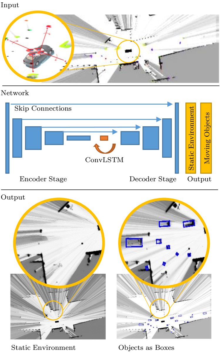
Figure 1: System Overview: The input is a dynamic occupancy grid map, shown as excerpt in the first row. The second row depicts the employed neural network, containing a down sampling stage, a ConvLSTM cell, an upsampling stage and two heads as output. The resulting environment model is shown in the third row: The static environment as grid map where dynamic cells are removed by the network and moving objects as rotated rectangles.

The proposed system aims for an environment model containing static regions in a model-free representation and objects modeled as rectangles with position, shape and orientation. An overview of the system architecture is given in Fig. 1.

The dynamic occupancy grid map (DOGMa) from [6] serves as input to a neural network. The DOGMa can be seen as a full object-model-free environment representation based on Bayesian sensor fusion. Occupancy and velocity estimates for grid cells $c$ result from a particle filter. The cell channels $\Omega=\left\{M_{\mathrm{O}},M_{\mathrm{F}},v_{\mathrm{E}},v_{\mathrm{N}},\sigma^{2}_{v_{\mathrm{E}}},\sigma^{2}_{v_{\mathrm{N}}},\sigma^{2}_{v_{\mathrm{E}},v_{\mathrm{N}}}\right\}$ denote the Dempster-Shafer [23] masses for occupancy and free space, the velocity pointing east and north, as well as the velocity variances and covariances, respectively. In our grid illustrations, dark pixels refer to high occupancy probability, calculated with $P_{\mathrm{O}}=0.5\cdot M_{\mathrm{O}}+0.5\cdot(1-M_{\mathrm{F}})$. Occupancy probability at a grid cell $c$ and sequence time step $t$ is denoted by $P_{\mathrm{O}}(\mathrm{E},\mathrm{N},t):=P_{\mathrm{O}}(c,t)$. The DOGMa has width $W$ and height $H$, providing data in $\mathbb{R}^{W\times H\times|\Omega|}$ for each time step.

A convolutional neural network transforms the object-model-free dynamic representation of the DOGMa into a model-free representation of static regions and model-based representation of moving objects. The employed neural network is based on a simple encoder-decoder structure with skip connections [24]. A ConvLSTM [5] cell is included upstream to the decoder stage with the intention to accumulate information from the input sequence. Although the DOGMa particle filter provides information about dynamics in the scene, long-term sequence information accumulation by recurrent network cells can help to compensate long-term occlusions and non-Gaussian noise which is hard to overcome with common grid fusion. In addition, the convolutional LSTM cells are able to include context in sequential processing, while DOGMa cells are assumed to be independent in the particle filter. The DOGMa side length is $\mathrm{E}=\mathrm{N}=901$ while step-wise downscaling is performed in the encoder to $301$, $101$, $51$ and $26$. A $26\times 26\times 512$ tensor is fed to the LSTM cell with kernel size $5\times 5$ and $512$ output channels. The result is upscaled using deconvolution mirroring the downscaling stages.

Parallel network heads form the output of our environment model. The first output $\hat{y}^{(\mathrm{s})}$ is the occupancy probability of static regions provided in $\mathbb{R}^{W\times H\times 1}$. The $4$ output tensors $\hat{y}^{(\mathrm{IoU})}$, $\hat{y}^{(\Delta{w})}$, $\hat{y}^{(\Delta{l})}$ and $\hat{y}^{(\Delta{\phi})}$ yield object rectangles following the concept of anchors [25]. Anchors define a set of default boxes described by triples $\left(w,l,\phi\right)$, including box width, length and orientation, respectively. $\hat{y}^{(\mathrm{IoU})}$ provides a score in terms of the expected intersection-over-union (IoU), which is the Jaccard-Index, between a detected object and anchors. Relative offsets $\Delta{w}$, $\Delta{l}$ and $\Delta{\phi}$ between detected object rectangle and default anchor box are given in the remaining output tensors. We used the optimized anchors from [3], resulting in tensors $\hat{y}^{(\mathrm{IoU})}\in\mathbb{R}^{W\times H\times 120}$, $\hat{y}^{(\Delta{w})},\hat{y}^{(\Delta{l})}\in\mathbb{R}^{W\times H\times 10}$ and $\hat{y}^{(\Delta{\phi})}\in\mathbb{R}^{W\times H\times 12}$.

IV Automatic Label Generation

Labels are generated fully automatically using offline sequence processing. While real-time applications usually don’t refine past estimates, for our goal the whole sequence can be used to generate accurate labeling data. Instead of only relying on velocity estimates in the DOGMa, occupancy movement is analyzed as illustrated in Fig. 2.

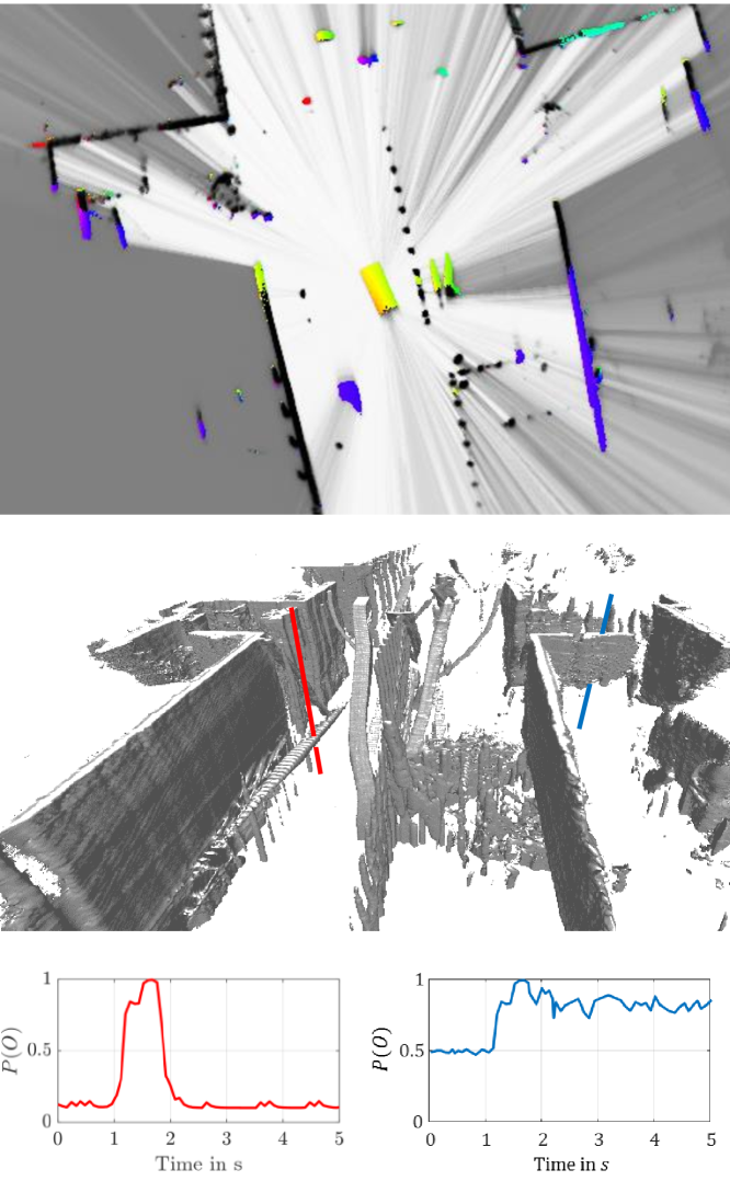
Figure 2: Offline sequence assessment: A single DOGMa time step contains false velocity estimation, as illustrated by colored pixels in the DOGMa (top row). In the 3D-graph (middle row), the grid map sequence is aligned using ego motion compensation. Occupancy probability of the two vertical lines (red and blue) is illustrated in the bottom row. The red curve illustrates $P_{\mathrm{O}}(t)$ caused by moving objects, while at the blue curve, static regions become uncovered causing false velocity estimates in the particle filter.

This enables us to overcome measurement noise and distinguish between actual moving objects and static objects with false velocity estimation. False velocity estimation in grid cells is mainly caused when static regions enter the field of view or become visible from previous occlusion. Therefore, we search for a pattern in the occupancy probability sequence of cells $P_{\mathrm{O}}(c,t)$: a raise of $P_{\mathrm{O}}$ followed by a fall. The resulting classification is directly used to train $\hat{y}^{(\mathrm{s})}$. For object labels, we first fit rectangles straight forward in dynamic regions, but refine their shape and orientation when the object was traced through the sequence. Furthermore, unreasonable trajectories are removed from the labeling data. A detailed description of offline object extraction can be found in [26].

V Training

V-A Loss Function

For the training of our deep neural network, we combine adapted versions of the loss functions from [4] and [3] to incorporate the segmentation of static and dynamic regions into the object detection process introduced in [3]. The total loss is given by

$$L=L_{s}+L_{d},$$ (1)

with static loss function $L_{s}$ and dynamic loss $L_{d}$. For the distinction between static and dynamic grid cells, the desired output is the probability of each cell being static or not. This task can be classified as a regression problem, thus we employ the basic Euclidean Loss (or L$2$-Loss) as the static loss function

$$L_{s}=\frac{\lambda_{s}}{2}\sum_{c}\left(\hat{y}_{s}(c)-y_{s}(c)\right)^{2},$$ (2)

where $\lambda_{s}$ denotes the static weighting factor. To tackle the high imbalance between dynamic and static grid cells, which is described in [4] and [3], the spatial balancing loss function

$$L_{d}=L_{d}^{(IoU)}+L_{d}^{(\Delta{w})}+L_{d}^{(\Delta{l})}+L_{d}^{(\Delta{\phi})}$$ (3)

is used [3]. Each term on the right hand side in (3) is given by

$$\begin{split}L_{d}^{(\cdot)}=\frac{\lambda_{d}^{(\cdot)}}{2}\sum_{c}\sum_{\alpha}(1+\lambda_{\mathrm{I}}\cdot\mathbf{A}(c)^{f_{d}})\\ \left(\hat{y}_{d}^{(\cdot)}(c,\alpha)-y_{d}^{(\cdot)}(c,\alpha)\right)^{2},\end{split}$$ (4)

where $y_{d}^{(\cdot)}\in\{y^{(\mathrm{IoU})}_{d},y^{(\Delta{w})}_{d},y^{(\Delta{l})}_{d},y^{(\Delta{\phi})}_{d}\}$ and $\lambda_{d}^{(\cdot)}$ denotes the weighting factor for each dynamic loss to adjust the influence of each output. To adjust the weighting of the cells, $\mathbf{A}(c)$ is used as a spatial map, where $\mathbf{A}(c)=0$ for all background cells and $0<\mathbf{A}(c)\leq 1$ for all cells that are occupied. The foreground gain $\lambda_{\mathrm{I}}$ reduces the aforementioned imbalance between background and object cells. Background cells are weighted by $1$, since $\mathbf{A}(c)=0$ and dynamic cells are weighted with a maximum of $1+\lambda_{\mathrm{I}}$. The focus parameter $f_{d}$ adjusts the weighting of the cells within the bounds of an object, e.g. $0<\mathbf{A}(c)\leq 1$. A more in-depth explanation of all parameters can be found in [3]. Furthermore, we add a regularization term with $\lambda_{R}=10^{-7}$ and dropout layers with a dropout rate of $r_{d}=0.1$ to avoid over-fitting, which was particular prevalent in the detection of small static regions as dynamic objects. For back-propagation and optimization the ADAM solver [27] was used due to its automatic learning rate update. The exponential decay rates for the ADAM algorithm are set to $\beta_{1}=0.9$ and $\beta_{2}=0.999$ and the starting learning rate is chosen to $l=0.0001$.

V-B Dataset

We collected about $2\,$\mathrm{h}$$ of data during multiple days in an urban shared space with pedestrians, other motor vehicles and bikes, while standing in the middle of the road on a parking lane. The labels were created with the automatic label generation algorithm introduced in [3]. The sequences contain a total of $78011$ images of which $68750$ were used for training, $8061$ for testing and $1200$ for the evaluation. The DOGMa, which is used as the input, has spatial dimensions of $901\times 901$ with a cell width of $0.15\,$\mathrm{m}$$.

We showed in [3], that on average, the ratio of occupied to free cells in our dataset is about $1:31$, the ratio of occupied to not occupied is about $1:65$ and the ratio of dynamic foreground cells to total occupied background cells is $1:400$. Furthermore, we also discovered an extreme imbalance between labels with $y^{(\mathrm{IoU})}=0$ and $y^{(\mathrm{IoU})}>0$ and even a high imbalance between $0<y^{(\mathrm{IoU})}<0.5$ and labels with $y^{(\mathrm{IoU})}\geq 0.5$. To reduce these imbalances, we chose the balanced loss functions and set the foreground gain to $\lambda_{\mathrm{I}}=400$, which is exactly the ratio of foreground to background cells, as described earlier. To counteract the differences within dynamic cells ($0<y^{(\mathrm{IoU})}<1$), the focus parameter is set to $f_{d}=4$. In comparison to the IoU label, the offset labels have equal values near the objects center and therefore, we conclude $f^{(\Delta{w})}_{d}=f^{(\Delta{l})}_{d}=f^{(\Delta{\phi})}_{d}=1$. Additionally, we chose the remaining weighting parameters as follows: $\lambda_{d}^{(IoU)}=1,\lambda_{d}^{(\Delta{w})}=0.01,\lambda_{d}^{(\Delta{l})}=0.05,\lambda_{d}^{(\Delta{\phi})}=0.25$ and $\lambda_{d}^{(s)}=0.5$.

The training process was stopped after about $1.5$ epochs with a total of $120000$ iterations and a batch size of $1$.

VI Results and Evaluation

Figure 3: Overview of the scene with static and dynamic segmentation of cells depicted in yellow and black. Blue bounding boxes represent detected dynamic objects, while red boxes are the ground-truth labels. The ego vehicle is the yellow rectangle in the middle of the scene facing upwards.

For the evaluation, we use a dataset that was recorded on different days in the same shared space downtown environment as the training dataset. The scene is illustrated in Fig. 3. Again, pedestrians, other motor vehicles and bikes were present during the time of the recording. Due to the rather random behavior of all road users, e.g. crossing the road at arbitrary locations or disappearing behind walls, our neural network has to deal with occlusion and predict and track the movement of objects by exploiting the sequential input data. The dataset was recorded by four Velodyne VLP-16 and one IBEO LUX laser scanner. We obtain a $360^{\circ}$ perception of the environment with our sensor setup and captured data in the range of $200\,$\mathrm{m}$$ (with opening angle of $100^{\circ}$ and four layers) with the IBEO LUX laser scanner. The Velodyne VLP-16 provide 16 layers of laser measurements with a range of $100\,$\mathrm{m}$$. We use about $2\,$\mathrm{min}$$ from two sequences for the evaluation. At the end of this section we also show the results of the same network, that was trained with only the Dempster-Shafer masses for free space $M_{\mathrm{F}}$ and occupancy $M_{\mathrm{O}}$. Our current input is generated by Bayesian sensor fusion and provides not only the masses but also the velocities and the corresponding variances for each cell.

To asses the performance of our classifier for the decision between dynamic and static cells, the receiver operator characteristic (ROC) curve is plotted in Fig. 4 by varying the threshold for the IoU between $0.01$ and $1$ and examining the true positive rate and the false positive rate. The area under curve (AUC) score for the classifier is $0.9463$, with values between $0.9$ and $1$ usually denoting an excellent classification result. However, this segmentation is an easy task for most artificial neural networks and many cells have an occupancy probability of $P_{\mathrm{O}}=0.5$, which means that their state is unknown. Nevertheless, the classifier yields satisfactory results in significant regions, which can be seen in Figure 3, where yellow cells show the static regions, black cells represent free space and red cells are dynamic objects.

Figure 4: Receiver operating characteristic curve (ROC) for segmentation between static and dynamic cells. The gray dashed line is the line of no-discrimination, which is equal to random guessing. The greater the distance between this line and the ROC curve, the better the classifier.

TABLE I: Bounding box error (RMSE) and average precision (AP)

	width	length	position	orientation	AP
old	$0.20\,$\mathrm{m}$$	$0.70\,$\mathrm{m}$$	$0.48\,$\mathrm{m}$$	$8.9^{\circ}$	$0.75$
new	$0.18\,$\mathrm{m}$$	$0.57\,$\mathrm{m}$$	$0.43\,$\mathrm{m}$$	$9.1^{\circ}$	$0.78$

To evaluate our results against our previous approach, the precision recall curve for the network with only a CNN and the new network combining a CNN and RNN is depicted in Fig. 5. The curve shows the object detection performance and was created by varying the threshold for the IoU between $0.01$ and $1$ and calculating the precision and the true positive rate (recall). We gain a slight but consistent improvement with our proposed network structure compared to our old approach for every IoU threshold with an average precision of $0.78$ in contrast to $0.75$. Furthermore, the root mean square errors for the position, width, length and orientation of the bounding boxes of our old and our new network are listed in Table I. The position, width and length estimates are improved due to the temporal filtering of the LSTM cell. To demonstrate these effects, two exemplary scenes are illustrated in Fig. 6 and 7, that correspond to the regions $1$ and $2$ in Fig. 3 respectively. Fig. 6 shows the results for an object that gets occluded by another one. The top row depicts the previous approach, while the bottom row shows the result of our new proposed approach. With our recurrent neural network, the green and red objects are detected in all four time steps, even when the object in the front covers the one in the back. With only the CNN (top row), the network fails to detect the rear object when it gets occluded in time step $2$, even though it detected both objects in the first frame. This misbehavior may be traced back to not having a memory of previous time steps, where our new approach remembers a detected object and tracks it over time. Another advantage of the memory is the consistency of the size estimates of the bounding boxes. When our old network loses a detection in the second frame and detects it again in the third frame, it has no knowledge about its past state and both the dimension and orientation estimates get worse. Again, the old approach fails to detect the green object in time step $4$. This behavior can lead to accidents in the real world, when dynamic obstacles like cars or pedestrians get overlooked by the object detection algorithm. Additionally, the varying size estimation can also be observed in the second scene in Fig. 7, where a far distant perception is depicted. The RNN tracks the moving object and keeps its size consistent over time, while the network without memory loses the detection in the second frame. Furthermore, the network underestimates the dimensions before getting the correct size again in the last time step. A wrong size estimation is particular hazardous for, e.g., behavior or trajectory planning and prediction, when the system assumes free space but in reality the object dimensions were wrongfully estimated.

Figure 5: Comparison of object detection precision recall curves between our previous approach and the new contribution with a CNN and a RNN.

In addition to our proposed method, we also conducted a preliminary experiment without the velocity channels obtained from the particle filter as input. Only the masses for occupancy $(M_{\mathrm{O}})$ and free space $(M_{\mathrm{F}})$ were used to train the network. Note that for the calculation of the masses the velocities were used, however, they are not fed explicitly to the network anymore. An exemplary scene from this experiment is depicted in Fig. 8. The results confirm that relevant features can be extracted from the Dempster-Shafer masses alone, so that objects are detected and parameterized. The object hypotheses are promising and show satisfactory and consistent bounding boxes in comparison to the ground-truth labels. However, one limitation so far, is the misclassification of dynamic and static cells without information about the dynamics of the scene.

Figure 6: Excerpt of the grid map in front of the ego-vehicle. The top sequence shows the result of our old approach, while the bottom sequence was created with our new approach. The green and red objects, that are detected in the first frame in both approaches, are of interest. In time step $2$ of our old method, the green object is occluded by the red object and is not detected, which is visualized by the green circle and the red lightning bold symbol. In time step $3$ the green object is detected again with a different size and orientation estimate. Furthermore, the red detection is lost, which is again visualized by the red circle and the lightning bold symbol. In the last frame (time step $4$), the green object is occluded and misdetected again. With our new approach, both the green and red objects are continuously detected in the bottom sequence in all frames and have a more consistent size estimate.

Figure 7: Far distant perception of the environment (about $50\,$\mathrm{m}$$ behind the ego-vehicle). The top sequence shows our old approach and the bottom sequence depicts the results of our new method. The green object, that is detected with both approaches in the first time step is of interest. With our old network, the detection is lost in time step $2$ due to very few measurements and is picked up again in time step $3$ with an obvious wrong size estimation. This is visualized by the red lightning bold symbol. Again, with our new approach, we get a continuous detection of the green object during the whole sequence shown in the bottom row. Additionally, the consistency of the size estimate is improved significantly.

Figure 8: Excerpt of the results without velocities at input. Objects detected by the network are depicted as blue bounding boxes and ground-truth labels are shown as black rectangles. The results show satisfactory and unvarying object hypotheses, that are consistent with the ground-truth labels. The estimation of static and dynamic cells fails. Most of the cells are estimated as dynamic (red regions), which obviously is a false classification.

VII Conclusion

In this paper, we presented a new deep learning approach to obtain the size, position and orientation of dynamic objects, represented as bounding boxes, as well as a pixel-wise segmentation of dynamic and static cells. We build on our previous network structure and extended it with a convolutional LSTM cell. This way, we are able to use memory to track objects states over time and overcome the problem of short occlusions and gain an enhanced object detection performance. Furthermore, the LSTM cell improves the consistency of size and position estimates, because previous knowledge about the object states is used for sequential filtering. Besides the LSTM cell, we included the classification of static and dynamic cells into our environment model, thus increasing the information value of our representation.

In the future, we wish to use raw measurements as input instead of a dynamic occupancy grid map constructed through Bayesian sensor fusion, thus employing an end-to-end learning approach. Our experiment using only the masses for free and occupied space without the velocities showed promising object detection results, that we wish to improve upon. Furthermore, for future work, parametric free space should be learned by the network, which is currently not possible with the proposed network structure. Finally, the extension of our work to use data from a moving vehicle can be considered.

References

- [1] F. Kunz, et al., “Autonomous driving at ulm university: A modular, robust, and sensor-independent fusion approach,” in IEEE Intelligent Vehicles Symposium, June 2015, pp. 666–673.
- [2] A. Elfes, “Occupancy grids: A stochastic spatial representation for active robot perception,” in Proceedings of the Sixth Conference on Uncertainty in AI, vol. 2929, 1990, p. 6.
- [3] S. Hoermann, et al., “Object Detection on Dynamic Occupancy Grid Maps Using Deep Learning and Automatic Label Generation,” ArXiv e-prints, Jan. 2018.
- [4] S. Hoermann, M. Bach, and K. Dietmayer, “Dynamic occupancy grid prediction for urban autonomous driving: A deep learning approach with fully automatic labeling,” CoRR, vol. abs/1705.08781, 2017. [Online]. Available: http://arxiv.org/abs/1705.08781
- [5] X. Shi, et al., “Convolutional LSTM network: A machine learning approach for precipitation nowcasting,” CoRR, vol. abs/1506.04214, 2015. [Online]. Available: http://arxiv.org/abs/1506.04214
- [6] D. Nuss, et al., “A random finite set approach for dynamic occupancy grid maps with real-time application,” arXiv preprint arXiv:1605.02406, 2016.
- [7] M. Schreier, V. Willert, and J. Adamy, “Compact representation of dynamic driving environments for adas by parametric free space and dynamic object maps,” IEEE Transactions on Intelligent Transportation Systems, vol. 17, no. 2, pp. 367–384, 2016.
- [8] A. Elfes, “Using occupancy grids for mobile robot perception and navigation,” Computer, vol. 22, no. 6, pp. 46–57, 6 1989.
- [9] K. M. Wurm, et al., “Octomap: A probabilistic, flexible, and compact 3d map representation for robotic systems,” in Proc. of the ICRA 2010 workshop on best practice in 3D perception and modeling for mobile manipulation, vol. 2, 2010.
- [10] P. Fankhauser and M. Hutter, “A Universal Grid Map Library: Implementation and Use Case for Rough Terrain Navigation,” in Robot Operating System (ROS) – The Complete Reference (Volume 1), A. Koubaa, Ed. Springer, 2016, ch. 5. [Online]. Available: http://www.springer.com/de/book/9783319260525
- [11] M. Schreier, V. Willert, and J. Adamy, “Grid mapping in dynamic road environments: Classification of dynamic cell hypothesis via tracking,” in Robotics and Automation (ICRA), 2014 IEEE International Conference on. IEEE, 2014, pp. 3995–4002.
- [12] F. Piewak, et al., “Fully convolutional neural networks for dynamic object detection in grid maps,” in 2017 IEEE Intelligent Vehicles Symposium (IV), June 2017, pp. 392–398.
- [13] D. Kim, et al., “L-shape model switching-based precise motion tracking of moving vehicles using laser scanners,” IEEE Transactions on Intelligent Transportation Systems, vol. 19, no. 2, pp. 598–612, 2018.
- [14] M. Munz, K. Dietmayer, and M. Mahlisch, “A sensor independent probabilistic fusion system for driver assistance systems,” in 2009 12th International IEEE Conference on Intelligent Transportation Systems, Oct 2009, pp. 1–6.
- [15] F. Roos, et al., “Reliable orientation estimation of vehicles in high-resolution radar images,” IEEE Transactions on Microwave Theory and Techniques, vol. 64, no. 9, pp. 2986–2993, Sept 2016.
- [16] A. Scheel and K. Dietmayer, “Tracking Multiple Vehicles Using a Variational Radar Model,” ArXiv e-prints, Nov. 2017.
- [17] S. Ren, et al., “Faster r-cnn: Towards real-time object detection with region proposal networks,” in Advances in Neural Information Processing Systems 28, 2015, pp. 91–99.
- [18] K. He, et al., “Mask r-cnn,” in 2017 IEEE International Conference on Computer Vision (ICCV), Oct 2017, pp. 2980–2988.
- [19] Q. Gan, et al., “First step toward model-free, anonymous object tracking with recurrent neural networks,” arXiv preprint arXiv:1511.06425, 2015.
- [20] J. Dequaire, et al., “Deep tracking in the wild: End-to-end tracking using recurrent neural networks,” The International Journal of Robotics Research, 2017.
- [21] S. Hochreiter and J. Schmidhuber, “Long short-term memory,” Neural computation, vol. 9, no. 8, pp. 1735–1780, 1997.
- [22] G. Ning, et al., “Spatially supervised recurrent convolutional neural networks for visual object tracking,” in Circuits and Systems (ISCAS), 2017 IEEE International Symposium on. IEEE, 2017, pp. 1–4.
- [23] A. P. Dempster, “A generalization of bayesian inference,” in Classic works of the dempster-shafer theory of belief functions. Springer, 2008, pp. 73–104.
- [24] O. Ronneberger, P. Fischer, and T. Brox, “U-net: Convolutional networks for biomedical image segmentation,” in International Conference on Medical image computing and computer-assisted intervention. Springer, 2015, pp. 234–241.
- [25] W. Liu, et al., “Ssd: Single shot multibox detector,” in Computer Vision – ECCV 2016, 2016, pp. 21–37.
- [26] D. Stumper, et al., “Offline Object Extraction from Dynamic Occupancy Grid Map Sequences,” CoRR, vol. abs/1804.03933, 20178. [Online]. Available: https://arxiv.org/abs/1804.03933
- [27] D. P. Kingma and J. Ba, “Adam: A method for stochastic optimization,” CoRR, vol. abs/1412.6980, 2014. [Online]. Available: http://arxiv.org/abs/1412.6980