Dynamics of Kuramoto oscillators with time-delayed postitive and negative couplings

Abstract

Many real-world examples of distributed oscillators involve not only time delays but also attractive (positive) and repulsive (negative) influences in their network interactions. Here, considering such examples, we generalize the Kuramoto model of globally coupled oscillators with time-delayed positive and negative couplings to explore the effects of such couplings in collective phase synchronization. We analytically derive the exact solutions for stable incoherent and coherent states in terms of the system parameters allowing us to precisely understand the interplay of time delays and couplings in collective synchronization. Dependent on these parameters, fully coherent, incoherent states and mixed states are possible. Time-delays especially in the negative coupling seem to facilitate collective synchronization. In case of a stronger negative coupling than positive one, a stable synchronized state cannot be achieved without time delays. We discuss the implications of the model and the results for natural systems, particularly neuronal network systems in the brain.

Introduction. The Kuramoto model Kuramoto:1975 , originally formulated to simplify the Winfree’s biological oscillator model for the circadian rhythms of living systems Winfree:1967 , represents an analytically tractable model to study collective synchronization in large systems of coupled nonlinear oscillators. Since its conception, the Kuramoto model has been generalized to explain collective dynamical behaviors in many natural and technological systems of coupled nonlinear oscillators often with various coupling scenarios  Pikovsky:2001 ; Strogatz:2003 ; Rodrigues:2016 ; Boccaletti:2016 . As the nature is replete with beautiful complexities such as self-organized critical phenomena Bak:1996 arising from opposing forces, the interplay of positive-negative time-delayed interactions in the Kuramoto model of oscillators can also be expected to show rich dynamical behaviors yet to be investigated.

The generalizations of the Kuramoto model previously analyzed include coupling scenarios with separate time-delayed interactions, and positive as well as negative coupling. In an outstanding analytical work, Yeung and Strogatz Yeung:1999 considered time delay in a mean-field sinusoidal coupling of Kuramoto model and derived exact formulas for the stability boundaries of the incoherent and synchronized states as a functional of the delay in a special case where the oscillators were identical. Later, Earl and Strogatz Earl:2003 extended the analysis to a variety of coupling topologies (regular, small-world and random network graphs) to find that the same stability criterion held true as for the mean-field case. In another more recent study, Hong and Strogatz Hong:2011 ; Hong:2011b studied the Kuramoto model with positive and negative coupling parameters (without time-delay) and reported a variety of dynamical behaviors including fully synchronized, partially synchronized, desynchronized and traveling states. Qui and colleagues Qui:2016 recently discovered a new non-stationary state (named Bellerophone) along with a synchronized state in the model with positive and negative coupling. However, the dynamics of the Kuramoto model with combined time-delayed interactions and positive-negative (attractive-replusive or excitatory-inhibitory) couplings have largely remained unexplored despite their relevance to many natural systems, such as biological, physical, chemical and social networks.

Interaction time-delays and excitation-inhibition (E-I) are usually characteristics of spatially distributed, self-organized systems, such as neurons in the brain in which the E-I balance is required to maintain normal temporal and spatial functional organization in healthy cognitive functions and behaviors WilsonCowen:1972 ; Wang:1996 ; Brunel:2003 ; Buzsaki:2006 ; Mann:2010 . Networks of coupled excitatory and inhibitory neurons can exhibit a complex dynamical behaviors including synchronization, multiclustered solutions, oscillator death Stefan:2008 . E-I couplings in Belousov-Zhabotinsky can lead to a large number of spatiotemporal patterns, simple to complex behaviors Vanag:2011 . In social networks of conformists (dynamical units with positive coupling) and contrarians (those with negative coupling) also, various collective behaviors are possible Galam:2004 ; Lama:2005 ; Hong:2011b . Interactions in spatially distributed oscillator network systems are not generally instantaneous. On the contrary, finite speed of signal transmission over a distance gives rise to a finite time delay. For example, signal transmission time delays are inherent in networks of neurons in the brain. While the chemical synaptic time delays are small ($\sim$2 ms), the axonal conduction delays, which depend on the distance between neurons in the brain, can reach upto tens of milliseconds Izhikevich:2006 . Time delays comparable to time-scales of neuronal oscillations are known to have significant effects in the collective (ensemble) activity of neurons Dhamala:2004 ; Izhikevich:2006 ; Adhikari:2011 . Time delays in networks of coupled inhibitory neurons can induce a variety of phase-coherent dynamic behaviors Liang:2009 . Time delays in networks with E-I can be expected to induce a variety of collective dynamical behaviors.

In this work, we analyze a generalized Kuramoto model of nonlinear oscillators with time-delayed positive and negative couplings for stability of coherent states and incoherent states and derive the exact analytical solutions to define the parameter boundaries for these states. As general results, we come to show that fully coherent, incoherent states and mixed states are possible, and time delays facilitate synchronized states in case of a stronger combined negative coupling than positive one.

Methods and results. We start with the following generalized Kuramoto model of $N$ oscillators globally connected with time-delayed positive and negative couplings:

$$\dot{\theta_{i}}(t)=w_{0}+\frac{k_{1}}{N_{1}}\sum_{j=1}^{N_{1}}f(\theta_{j}(t-\tau_{1})-\theta_{i}(t))$$

$$+\frac{k_{2}}{N_{2}}\sum_{j=N_{1}+1}^{N}f(\theta_{j}(t-\tau_{2})-\theta_{i}(t))$$ (1)

Here, the coupled system consists of $N_{1}$ and $N_{2}$ numbers of positively and negatively coupled oscillators. The total number is $N=N_{1}+N_{2}$, and $k_{1}+k_{2}=(1-c)k:=K$. $k$ is the coupling strength, $k_{1}$ is a positive coupling strength, $k_{2}$ is a negative coupling strength, and $c=k_{2}/k$ is the coupling ratio. $\theta_{i}(t)$ is the phase of the ith oscillator, $\dot{\theta_{i}}(t)$ its derivative and each oscillator has the same natural frequency $w_{0}$. $f$ is a general coupling function, which we replace with a sinusoidal function in our examples below. $\tau_{1}$ is the time delay associated with positive coupling and $\tau_{2}$ is the time delay with negative coupling. Below, we explore the interplay of the parameters ($k$, $c$, $\tau_{1}$ and $\tau_{2}$) in the emergence of stable coherent states.

The rest of the paper is organized as follows: (a) we analyzed the stability of a completely coherent state and derive the boundary curves for the coherent state, (b) we analyzed the stability of a completely incoherent state and derive the boundary curves for the in coherent state. In each case, we consider the following scenarios of delays (i)$\tau_{1}=\tau_{2}=\tau$, and (ii)$\tau_{1}=\tau>0$ and $\tau_{2}=0$. For the first case (a), we analyzed the time-evolution of a perturbation to a synchronized state. For the second case (b), we linearize the continuity equation around the incoherent state ($\rho(\theta,\omega,t)=1/2\pi$) describing the time-evolution of instantaneous phase distribution $\rho(\theta,\omega,t)$ on a unit circle, analyzed the effect of a perturbation on the incoherent state.

(a) Stability Analysis of coherent (synchronized) state. We assume the system reaches a complete synchronized state described by the following equation:

$$\theta_{i}(t)= \Omega t$$ (2)

The collective frequency $\Omega$ is given by

$$\Omega = w_{0}+k_{1}f(-\Omega\tau_{1})+k_{2}f(-\Omega\tau_{2})$$ (3)

Now, we add a small perturbation term on (2):

$$\theta_{i}(t)= \Omega t+\epsilon\phi_{i}(t),$$ (4)

where $0<\epsilon\ll 1$. Now, if we define $\Delta_{i}(t):=\phi_{i}(t)-\phi_{1}(t)$:

$$\dot{\Delta}_{i}(t) = -\frac{k_{1}}{N_{1}}f^{\prime}(-\Omega\tau_{1})\sum_{j=1}^{N_{1}}\Delta_{i}(t)-\frac{k_{2}}{N_{2}}f^{\prime}(-\Omega\tau_{2})\sum_{j=N_{1}+1}^{N}\Delta_{i}(t)$$ (5)

$$= -[k_{1}f^{\prime}(-\Omega\tau_{1})+k_{2}f^{\prime}(-\Omega\tau_{2})]\Delta_{i}(t)$$

The stability requirement for synchronization is that $\Delta_{i}(t)$ be decaying to zero instead of diverging to infinity. Hence,

$$k_{1}f^{\prime}(-\Omega\tau_{1})+k_{2}f^{\prime}(-\Omega\tau_{2})>0$$ (6)

When (6) is satisfied for $\forall i=1,2,3,...N$, $\phi_{i}(t)$ exponentially converges to the same function $\phi(t)$. Thus, $\phi(t)$ satisfies the following time delay equation:

$$\dot{\phi}(t)=\frac{k_{1}}{N_{1}}f^{\prime}(-\Omega\tau_{1})\sum_{j=1}^{N_{1}}[\phi(t-\tau_{1})-\phi(t)]$$

$$+\frac{k_{2}}{N_{2}}f^{\prime}(-\Omega\tau_{2})\sum_{j=N_{1}+1}^{N}[\phi(t-\tau_{2})-\phi(t)]$$ (7)

If we let $\tau_{1}=\tau_{2}=\tau$ for a synchronization state, we have

$$(1-c)f^{\prime}(-\Omega\tau)>0$$ (8)

$$\dot{\phi}(t)=(1-c)kf^{\prime}(-\Omega\tau)[\phi(t-\tau)-\phi(t)]$$

With $\phi(t)=e^{\lambda t}$ to find the characteristic function, we have

$$\lambda=(1-c)kf^{\prime}(-\Omega\tau)(e^{-\lambda\tau}-1)$$ (9)

A brief analysis shows that when (8) is satisfed, for this type of characteristic function and $\lambda\neq 0$, all eigenvalues have negative real parts, i. e. $Re(\lambda)<0$ (stable state).

If we let $\tau_{1}=\tau>0$, $\tau_{2}=0$, (6) becomes

$$f^{\prime}(-\Omega\tau)-cf^{\prime}(0)>0$$ (10)

We now let the general coupling function to be a sinusoidal, $f(\theta)=\sin(\theta)$, for $\tau_{1}=\tau_{2}=\tau$ and we arrive at the following two cases: (i) if $1-c>0$, then $\cos(\Omega\tau)>0$, and (ii) if $1-c<0$, then $\cos(\Omega\tau)<0$.

We let $T=\frac{2\pi}{\omega_{0}}$, $y=\frac{k}{\omega_{0}}$ and arrive at the solutions for the boundary curves of the unstable coherent states in two cases: (i) when $1-c>0$, we have

$$\frac{4n+1}{4(1-(1-c)y)}<\frac{\tau}{T}<\frac{4n+3}{4(1+(1-c)y)}$$ (11)

and $0<y<\frac{1}{2(1-c)(2n+1)}$.

and (ii) when $1-c<0$, we have

$$\frac{4n-1}{4(1+(1-c)y)}<\frac{\tau}{T}<\frac{4n+1}{4(1-(1-c)y)}$$ (12)

and $0<y<\frac{1}{4n(c-1)}$. We use $(\ref{eq:20})$ and $(\ref{eq:21})$ to draw the boundary curves and areas for unstable synchronized states, as shown in black shades of Fig. 1(a).

We now consider $f(\theta)=\sin(\theta)$, $\tau_{1}=\tau>0$, $\tau_{2}=0$. According to $(\ref{eq:12})$,

$$\cos(\Omega\tau)-c>0$$ (13)

is required to have a stable solution. This solution $(\ref{eq:12})$ implies that a time delay is needed for a stable synchronization in case of a stronger negative coupling ($c>1$). When $\cos(\Omega\tau)-c>0$, $\forall i=1,2,...N$: $\phi_{i}(t)$ exponentially converges to the same $\phi(t)$, $\phi(t)$ then satisfies the following equation:

$$\dot{\phi}(t)=k\cos(\Omega\tau)[\phi(t-\tau)-\phi(t)]$$

Then, the characteristic function satisfies:

$$\lambda=k\cos(\Omega\tau)(e^{-\lambda\tau}-1)$$ (14)

It is easy to show that for any $k>0$ and $\cos(\Omega\tau)>c$, for all $\lambda\neq 0$, $Re(\lambda)<0$. Therefore, the synchronization state is always linearly stable. Whenever $c\geq 1$, we do not have a stable coherent state. Taking $y=\frac{k}{\omega_{0}}$, $T=\frac{2\pi}{\omega_{0}}$, when $0<c<1$, there is no stable synchronization state if and only if $\tau$ satisfies following inequality:

$$\frac{2n\pi+arc\cos c}{2\pi(1-\sqrt{1-c^{2}}y)}<\frac{\tau}{T}<\frac{2(n+1)\pi-arc\cos c}{2\pi(1+\sqrt{1-c^{2}}y)}$$ (15)

and

$$0<y<\frac{\pi-arc\cos c}{(2n+1)\pi\sqrt{1-c^{2}}}$$ (16)

We use $(\ref{eq:24})$ and $(\ref{eq:26})$ to draw the boundary curves and areas for this unstable coherent state, as shown with black shade in Fig. 1(b).

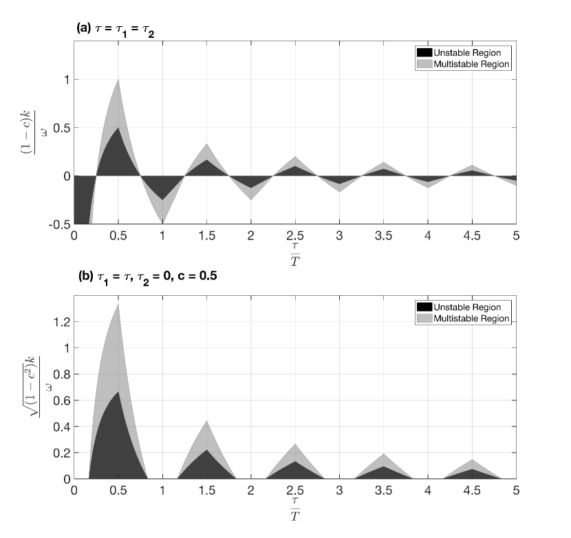
Figure 1: Regions of unstable coherent and stable incoherent states (dark shade), stable coherent and incoherent states (gray), and stable coherent state (unshaded or white) as a function of coupling strength and time delay. These boundaries of stability obtained by the analytical solutions were also numerically verified.

(b) Stability analysis of incoherent state.

We now approach the stability of incoherent state, from equation (Dynamics of Kuramoto oscillators with time-delayed postitive and negative couplings), by considering the mean field of positive oscillators and the mean field of negative oscillators:

$$r_{1}e^{i\phi_{1}} = \frac{1}{N_{1}}\sum_{j=1}^{N_{1}}e^{i\theta_{j}}$$

$$r_{2}e^{i\phi_{2}} = \frac{1}{N_{2}}\sum_{j=N_{1}+1}^{N_{1}+N_{2}=N}e^{i\theta_{j}}$$ (17)

The conditional probability density function $\rho(\theta,\omega,t)$ satisfies

$$\int_{0}^{2\pi}\rho(\theta,\omega,t)d\theta=1$$ (18)

For complete incoherent state:

$$\rho(\theta,\omega,t)=\frac{1}{2\pi}$$ (19)

For $\forall$ $i=1,2,3,...N$,

$$r_{1}e^{i(\phi_{1}(t-\tau_{1})-\theta_{i}(t))}=\frac{1}{N_{1}}\sum_{j=1}^{N_{1}}e^{i(\theta_{j}(t-\tau_{1})-\theta_{i}(t))}$$ (20)

Similarly,

$$r_{2}e^{i(\phi_{2}(t-\tau_{2})-\theta_{i}(t))}=\frac{1}{N_{2}}\sum_{j=N_{1}+1}^{N}e^{i(\theta_{j}(t-\tau_{2})-\theta_{i}(t))}$$ (21)

Considering the imaginary part of (20) and (21), we can transfer the dynamical equation in the mean field form as:

$$\dot{\theta_{i}}(t)=\omega_{i}+k_{1}r_{1}\sin(\theta_{j}(t-\tau_{1})-\theta_{i}(t))$$

$$+k_{2}r_{2}\sin(\theta_{j}(t-\tau_{2})-\theta_{i}(t))$$ (22)

The equation with a perturbation to the incoherent state is then:

$$\rho(\theta,\omega,t)=\frac{1}{2\pi}+\epsilon\eta(\theta,\omega,t)$$ (23)

with $\epsilon\ll 1$.

Here $\eta(\theta,\omega,\tau)$ can be expanded into following Fourier series:

$$\eta(\theta,\omega,t)=c(\omega,t)e^{i\theta}+c^{*}(\omega,t)e^{-i\theta}+\eta^{\perp}(\theta,\omega,t)$$ (24)

Here, $\eta^{\perp}$ are higher Fourier Harmonics. We now look for a type of solution of the form:

$$c(\omega,t)=b(\omega)e^{\lambda t}$$ (25)

$$\lambda b(\omega)=-i\omega b(\omega)+\frac{k_{1}e^{-\lambda\tau_{1}}}{2}\int_{-\infty}^{\infty}b(v)g(v)dv$$

$$+\frac{k_{2}e^{-\lambda\tau_{2}}}{2}\int_{-\infty}^{\infty}b(v)g(v)dv$$ (26)

For identical frequencies, $\omega_{i}=\omega_{0}$, $\forall i=1,2,...N$, $g(\omega)=\delta(\omega-\omega_{0})$, $\delta$ is the dirac delta function.

The eigenvalue $\lambda$ satisfies the following equation:

$$\lambda+i\omega_{0}=\frac{1}{2}(k_{1}e^{-\lambda\tau_{1}}+k_{2}e^{-\lambda\tau_{2}})$$ (27)

When $\tau_{1}=\tau_{2}=\tau$, $k_{1}=k>0$, $k_{2}=-ck<0$, $c>0$ is a constant,

$$(1-c)k=2(\lambda+i\omega_{0})e^{\lambda\tau}$$ (28)

At a critical (bifurcation) point $K_{c}$, the eigenvalue $\lambda$ passes through the imaginary axis $\lambda=Ri$, $R$ is real number.

From the equation above, $2(\lambda+i\omega_{0})e^{\lambda\tau}=2i(R+\omega_{0})(\cos(R\tau)+i\sin(R\tau))$ has to be a real value. Hence, $\cos(R\tau)=0$. If we take $R\tau=(-m+\frac{1}{2})\pi$, $m\in Z$.

$$(1-c)k=2(-1)^{m-1}(R+\omega_{0})$$ (29)

$$2\omega_{0}\tau+(-1)^{m}(1-c)k\tau=-2R\tau$$

$$=2(m-\frac{1}{2})\pi=(2m-1)\pi$$ (30)

Taking $m=2n+1$ odd positive integers, we get one boundary for $\tau$:

$$\tau_{c1}=\frac{(4n+1)\pi}{2\omega_{0}-(1-c)k}$$ (31)

If we take $m=2n$ or $m=2(n+1)$ even positive integers, we get other boundaries for $\tau$:

$$\tau_{c2}=\frac{(4n-1)\pi}{2\omega_{0}+(1-c)k}$$ (32)

$$\tau_{c3}=\frac{(4n+3)\pi}{2\omega_{0}+(1-c)k}$$ (33)

Letting $T=\frac{2\pi}{\omega_{0}}$, $y=\frac{k}{w_{0}}$, for $(1-c)k=K>0$ and $\tau_{c1}<\tau<\tau_{c3}$, we have the stable incoherent state within:

$$\frac{4n+1}{4(1-\frac{(1-c)y}{2})}<\frac{\tau}{T}<\frac{4n+3}{4(1+\frac{(1-c)y}{2})}$$ (34)

For $(1-c)k=K<0$, $\tau_{c2}<\tau<\tau_{c1}$, we have the stable incoherent state within:

$$\frac{4n-1}{4(1+\frac{(1-c)y}{2})}<\frac{\tau}{T}<\frac{4n+1}{4(1-\frac{(1-c)y}{2})}$$ (35)

We use $(\ref{eq:56-01})$ and $(\ref{eq:56-02})$ to draw the boundary curves and areas for this unstable incoherent state, as shown with grey shade in Fig. 1(a).

For $\tau_{1}=\tau>0$, $\tau_{2}=0$, the eigenvalue $\lambda$ has to satisfy the following equation:

$$\lambda+i\omega_{0}=\frac{1}{2}(k_{1}e^{-\lambda\tau}+k_{2})$$ (36)

If $c\geq 1$, let $\lambda=\alpha+iR$, $\alpha,R$ are real.

$$k(e^{-\alpha\tau}\cos(R\tau)-c)=2\alpha$$ (37)

It is easy to see that when $c>1$, $(\ref{eq:59})$ requires $\alpha<0$, while $c=1$ and $\alpha\geq 0$, then the only possibility to satisfy $(\ref{eq:59})$ is $\alpha=R=0$. So, the incoherent state is always neutrally stable whenever $c\geq 1$. An unstable incoherent state only possibly exist for $0<c<1$.

At a bifurcation point, $\lambda=Ri$, R is real. Substituting it to $(\ref{eq:57})$:

$$2(R+\omega_{0})i=k(\cos(\tau R)-i\sin(\tau R))-ck$$ (38)

$$(2R+2\omega_{0}+k\sin(\tau R))i=k(\cos(\tau R)-c)$$ (39)

The above equation is satified if and only if $\cos(\tau R)=c$ and

$$k\sin(\tau R)=-2(R+\omega_{0})$$ (40)

$\tau R=-2m\pi\pm arc\cos c$, $m$ are integers. $\sin(\tau R)=\pm\sqrt{1-c^{2}}$.

$$k=\mp\frac{2(R+\omega_{0})}{\sqrt{1-c^{2}}}$$ (41)

If we take $m=n$ and $\tau R=-2n\pi-arc\cos c$, we get the left boundary for $\omega_{0}\tau$ as:

$$\omega_{0}\tau_{lc}=2n\pi+arc\cos c+\frac{1}{2}k\tau\sqrt{1-c^{2}}$$ (42)

Similarly, if take $m=n+1$ and $\tau R=-2n\pi+arc\cos c$, we get the right boundary for $\omega_{0}\tau$ as:

$$\omega_{0}\tau_{rc}=2(n+1)\pi-arc\cos c-\frac{1}{2}k\tau\sqrt{1-c^{2}}$$ (43)

The incoherent state is stable if and only if $\omega_{0}\tau_{lc}<\omega_{0}\tau<\omega_{0}\tau_{rc}$. If make $y=\frac{k}{\omega_{0}}$, we have

$$\frac{2n\pi+arc\cos c}{2\pi(1-\frac{\sqrt{1-c^{2}}y}{2})}<\frac{\tau}{T}<\frac{2(n+1)\pi-arc\cos c}{2\pi(1+\frac{\sqrt{1-c^{2}}y}{2})}$$ (44)

We use $(\ref{eq:65})$ and $(\ref{eq:67})$ to draw the boundary curves and areas for this unstable incoherent state, as shown with grey shade in Fig. 1(b).

Finally, we have also numerically verified all these analytical results of Fig.1(a,b).

Conclusions and discussion. Here, we generalize the Kuramoto model of globally coupled phase oscillators with time-delayed positive-negative coupling. We have analytically and numerically studied the stability of synchronized and incoherent states in this generalized Kuramoto model. We derive the exact solutions for the critical coupling strengths at different time delays for stable incoherent and coherent states. These derivations proivde new insights into how the interplay of time delays can affect collective synchronization. We find that fully coherent, incoherent and mixed states are possible dependent on the parameters in this generalized model. Time delayed interactions are helpful for achieving synchronization in the case of dominant negative network coupling. We expect that our theoretical work will be useulf for further research in trying to understand the role of excitation-inhibition in self-organized systems of distributed oscillators like the neuronal systems in the brain.

References

- (1) Y. Kuramoto, in Proceedings of the International Symposium on Mathematical Problems in Theoretical Physics, edited by H. Araki, Lecture Notes in Physics Vol. 39 (Springer, Berlin, 1975); Chemical Oscillations, Waves, and Turbulence (Springer, Berlin, 1984).
- (2) A. T. Winfree, J. Theor. Biol. 16, 15 (1967).
- (3) A. Pikovsky, M. Rosenblum, J. Kurths, in Synchronization: a Universal Concept in Nonlinear Sciences, Cambridge University Press, Cambridge, England, 2001).
- (4) S. Strogatz, Sync: The emerging science of spontaneous order (Hyperion, New York, 2003).
- (5) F. A. Rodrigues, T. K. DM. Peron, P. Ji, and J. Kurths, Phys. Rep. 610, 1 (2016).
- (6) S. Boccaletti, J. A. Almendral, S. Guan, I. Leyva, Z. Liu, I. Sendina-Nadal, Z. Wang, and Y. Zou, Phys. Rep. 660, 1 (2016).
- (7) P. Bak, How nature works: the science of self-organized criticality (Springer-Verlag, New York, 1996).
- (8) M. K. Stephen Yeung, S. H. Strogatz, Phys. Rev. Lett. 82, 648 (1999).
- (9) M. G. Earl, S. H. Strogatz, Phys. Rev. E 67, 036204-1 (2003).
- (10) H. Hong, S. H. Strogatz, Phys. Rev. Lett. 106, 054102 (2011).
- (11) H. Hong, S. H. Strogatz, Phys. Rev. E 84, 046202 (2011).
- (12) T. Qui, S. Boccaletti, I. Bonamassa, Y. Zou, J. Zhou, Z. Liu, S. Guan, Sci. Rep. 6, 36713 (2016).
- (13) H. R. Wilson, J. D. Cowan, Biophys. J. 12, 1 (1972).
- (14) X. J. Wang, G. Buzsáki, J. Neurosci. 16, 6402 (1996).
- (15) N. Brunel, X. J. Wang, J. Neurophysiol. 90, 415–430 (2003).
- (16) G. Buzsaki, in Rhythms of the Brain, (Oxford University Press, Cambridge, England, 2006).
- (17) E. O. Mann, I. Mody, Nat. Neurosci. 13, 205 (2010).
- (18) V. K. Vanag, I. R. Epstein, Phys. Rev. E 84 066209 (2011).
- (19) R. A. Stefanaescu, V. K. Jirsa, PLOS Comp. Biol. 4, e1000219 (2008).
- (20) S. Galam, Physica A 333, 453 (2004).
- (21) M. S. Lama, J. M. Lopez, H. S. Wio, Europhys. Lett. 72, 851 (2005).
- (22) E. M. Izhikevich, Neural Comput 18, 245-282 (2006).
- (23) B. M. Adhikari, A. Prasad, M. Dhamala, Chaos 21, 023116 (2011).
- (24) M. Dhamala, V. K. Jirsa, M. Ding, Phys Rev Lett 92, 074104 (2004).
- (25) X. Liang, M. Tang, M. Dhamala, and Z. Liu, Phys. Rev. E 80, 066202 (2009).