Control the model sign problem via path optimization method:
Monte-Carlo approach to QCD effective model with Polyakov loop

Abstract

We apply the path optimization method to a QCD effective model with the Polyakov loop at finite density to circumvent the model sign problem. The Polyakov-loop extended Nambu–Jona-Lasinio model is employed as the typical QCD effective model and then the hybrid Monte-Carlo method is used to perform the path integration. To control the sign problem, the path optimization method is used with complexification of temporal gluon fields to modify the integral path in the complex space. We show that the average phase factor is well improved on the modified integral-path compared with that on the original one. This indicates that the complexification of temporal gluon fields may be enough to control the sign problem of QCD in the path optimization method.

I Introduction

Investigation of the phase structure of Quantum Chromodynamics (QCD) is one of the important subjects in the study of the hot and dense QCD matter. If we directly obtain the phase diagram at finite temperature ($T$) and density from the first-principles calculation such as the lattice QCD simulation, there are no fog in the exploration. Lattice QCD, however, has the sign problem at finite real chemical potential ($\mu$) and then we cannot obtain the reliable results at finite density. To circumvent the sign problem, several methods have been proposed such as the Taylor expansion method Miyamura et al. (2002); Allton et al. (2005); Gavai and Gupta (2008), the reweighting method Fodor and Katz (2002a); *Fodor:2001pe; *Fodor:2004nz; Fodor et al. (2003), the analytic continuation method de Forcrand and Philipsen (2002); *deForcrand:2003hx; D’Elia and Lombardo (2003); *D'Elia:2004at; Chen and Luo (2005), the canonical approach Hasenfratz and Toussaint (1992); Alexandru et al. (2005); Kratochvila and de Forcrand (2006); de Forcrand and Kratochvila (2006); Li et al. (2010) and so on. However, we cannot go beyond the $\mu/T\sim 1$ line by using those methods; for example, see Ref. de Forcrand (2009).

Recently, new ideas have been applied to attack the sign problem such as the complex Langevin method Parisi and Wu (1981); Parisi (1983) and the Lefschetz-thimble method Witten (2011); Cristoforetti et al. (2012); Fujii et al. (2013). Both methods are based on the complexification of dynamical variables. The complex Langevin method is based on the stochastic quantization and thus it does not have the sign problem, in principle. In the Lefschetz-thimble method, one should solve flow equations to construct the new integral path which is corresponding to the steepest descent trajectory; this trajectory is so called the Lefschetz thimble. Unfortunately, these methods have some serious problems and thus it is difficult to apply it to QCD at high density: In the complex Langevin method, there is the possibility that it is converged to wrong results due to the excursion and singular problems Aarts et al. (2010); Tanizaki et al. (2015). In comparison, the Lefschetz-thimble method has the global sign problem when multi Lefschetz-thimbles contribute to the path integral and then there is the serious cancellation between them; for example, see Ref. Fujii et al. (2013). In addition, we should evaluate the Jacobian induced by the modification of the integral path and it leads the serious increase of the numerical cost. Furthermore, the Jacobian induces the residual sign problem because the oscillation of the Boltzmann weight arises. Also, we may face the problem to draw thimbles when the classical or the effective action has singular points Mori et al. (2017a).

In Ref. Mori et al. (2017b), we have proposed the new method which we call the path optimization method (POM) motivated by the Lefschetz-thimble method. The path optimization method is strongly improved in Ref. Mori et al. (2018) by introducing the feedforward neural network to optimize the modified integral path. In this method, we first complexify the variables of integration as in the Lefschetz-thimble method. Then, the modified integral path is constructed to minimize the cost function which reflects the seriousness of the sign problem. Therefore, we can treat the sign problem as the optimization problem. The sign problem in the simple one-dimensional integration Mori et al. (2017b); Ohnishi et al. (2017) and the complex $\lambda\phi^{4}$ theory Mori et al. (2018) are found to be under controlled. Unfortunately, the numerical cost of the path optimization method is still heavy and thus we cannot apply it to QCD yet, but this method has large extensibility compared with the Lefschetz-thimble method and thus we can still dream to apply it to QCD in the future.

Because of several difficulties in QCD as mentioned above, QCD effective models have been widely used to investigate the QCD phase structure because such effective model is much easier than original QCD. The Polyakov-loop extended Nambu–Jona-Lasinio (PNJL) model Meisinger et al. (2002); Fukushima (2004); Ratti et al. (2006) is one of the famous and powerful effective models. Unfortunately, the PNJL model has the model sign problem Fukushima and Hidaka (2007); Tanizaki et al. (2015) even in the mean-field approximation because one particular global minimum perfectly dominate the path integration and then the thermodynamic potential can be complex. It should be noted that this complex nature of the thermodynamic potential is not related with instabilities; the correct thermodynamic potential should be real.

In this study, we consider the PNJL model and the path optimization method to circumvent the model sign problem. This article is organized as follows. In Sec. II and III, we explain the formulation of the PNJL model and the path optimization method, respectively. The numerical results are shown in Sec. IV. Section V is devoted to summary.

II Formulation

In this work, we employ the PNJL model as the QCD effective model. The PNJL model can describe the chiral symmetry breaking/restoration and the approximate confinement-deconfinement transition. Also, it can well reproduce QCD properties at finite imaginary chemical potential which is a big advantage from the viewpoint of the topologically determined confinement-deconfinement transition Kashiwa and Ohnishi (2015, 2016, 2017). The following formulation and the computation of the Monte-Carlo PNJL model is based on Ref. Cristoforetti et al. (2010).

II.1 Polyakov-loop extended Nambu–Jona-Lasinio model

The Euclidean action of the PNJL model is

$$\Gamma_{\mathrm{PNJL}} =\int d^{4}x_{\mathrm{E}}\Bigl{[}{\bar{q}}(-i{\ooalign{\hfil/\hfil\crcr$D$}}+m_{0}-\mu\gamma_{0})q$$ (3)

$$-G\Bigl{\{}({\bar{q}}q)^{2}+({\bar{q}}i{\vec{\tau}}\gamma_{5}q)^{2}\Bigr{\}}\Bigr{]}-\beta V{\cal V}_{\Phi}(\Phi,{\bar{\Phi}}),$$ (4)

where $\beta=1/T$, $V$ is the three-dimensional spatial volume, $q$ denotes the two-flavor quark-fields, $m_{0}$ does the current quark mass, $D_{\nu}=\partial_{\nu}-iA_{\nu}\delta_{\nu 4}$, $G$ is the coupling constant of the four-fermi interaction, $\Phi$ (${\bar{\Phi}}$) means the Polyakov loop (its conjugate) and ${\cal V}_{\Phi}$ expresses the gluonic contribution.

With the homogeneous auxiliary-field ansatz after the Hubbard-Stratonovich transformation, the effective action is simplified as $\Gamma=\beta V{\cal V}$. Then, the effective potential is expressed as

$${\cal V} ={\cal V}_{\mathrm{NJL}}+{\cal V}_{\Phi},$$ (5)

where ${\cal V}_{\mathrm{NJL}}$ is the contributions of the NJL part. In the actual calculation, we employ the Polyakov gauge, $\partial_{4}A_{4}=0$.

The actual form of ${\cal V}_{\mathrm{NJL}}$ becomes

$${\cal V}_{\mathrm{NJL}} =-2N_{\mathrm{f}}\int_{\Lambda}\frac{d^{3}p}{(2\pi)^{3}}\Bigl{[}N_{\mathrm{c}}E_{\bf p}-N_{\mathrm{c}}\sqrt{{\bf p}^{2}+m_{0}^{2}}$$

$$+T\ln\Bigl{(}f^{-}f^{+}\Bigr{)}\Bigr{]}+G(\sigma^{2}+{\vec{\pi}}^{2}),$$ (6)

where $N_{\mathrm{f}}$ ($N_{\mathrm{c}}=3$) is the number of flavor (color), $\Lambda$ is the three-dimensional momentum cutoff and

$$f^{-} =1+3(\Phi+{\bar{\Phi}}e^{-\beta E_{\bf p}^{-}})e^{-\beta E_{\bf p}^{-}}+e^{-3\beta E_{\bf p}^{-}},$$

$$f^{+} =1+3({\bar{\Phi}}+\Phi e^{-\beta E_{\bf p}^{+}})e^{-\beta E_{\bf p}^{+}}+e^{-3\beta E_{\bf p}^{+}},$$ (7)

with $E_{\bf p}^{\mp}=E_{\bf p}\mp\mu=\sqrt{\varepsilon_{\bf p}^{2}+2N^{+}N^{-}}\mp\mu$ and $\varepsilon_{\bf p}=\sqrt{{\bf p}^{2}+M^{2}+N^{2}}$. The auxiliary fields are redefined as

$$M=m_{0}-2G\sigma,~{}~{}~{}N=-2G\pi^{0},~{}~{}~{}N^{\pm}=-2G\pi^{\pm}.$$ (8)

with $\pi^{0}=\pi_{3}$ and $\pi^{\pm}=(\pi_{1}\pm i\pi_{2})/\sqrt{2}$. The functional form of the Polyakov loop and its conjugate are

$$\Phi =\frac{1}{N_{\mathrm{c}}}\mathrm{tr}_{c}\Bigl{[}e^{i\beta A_{4}}\Bigr{]}=\frac{1}{N_{\mathrm{c}}}\Bigl{[}e^{i\beta\phi_{1}}+e^{i\beta\phi_{2}}+e^{i\beta\phi_{3}}\Bigr{]},$$

$${\bar{\Phi}} =\frac{1}{N_{\mathrm{c}}}\Bigl{[}e^{-i\beta\phi_{1}}+e^{-i\beta\phi_{2}}+e^{-i\beta\phi_{3}}\Bigr{]},$$ (9)

where

$$\phi_{1} =A_{3}+\frac{1}{\sqrt{3}}A_{8},~{}~{}~{}\phi_{2}=-A_{3}+\frac{1}{\sqrt{3}}A_{8}$$

$$\phi_{3} =-(\phi_{1}+\phi_{2})=-\frac{2}{\sqrt{3}}A_{8},$$ (10)

and then $A_{4}$ are diagonalized because we use the Polyakov gauge; $A_{4}=\mathrm{diag}(A_{3}+A_{8}/\sqrt{3},-A_{3}+A_{8}/\sqrt{3},-2A_{8}/\sqrt{3})$.

In this paper, we choose the logarithmic Polyakov-loop potential Roessner et al. (2007) as the gluonic contribution;

$$\frac{{\cal V}_{\Phi}}{T^{4}} =-\frac{1}{2}a_{T}{\bar{\Phi}}\Phi+b_{T}\ln(h),$$ (11)

where

$$h =1-6{\bar{\Phi}}\Phi+4({\bar{\Phi}}^{3}+\Phi^{3})-3({\bar{\Phi}}\Phi)^{2},$$ (12)

with

$$a_{T} =a_{0}+a_{1}\Bigl{(}\frac{T_{0}}{T}\Bigr{)}+a_{2}\Bigl{(}\frac{T_{0}}{T}\Bigr{)}^{2},~{}~{}~{}b_{T}=b_{3}\Bigl{(}\frac{T_{0}}{T}\Bigr{)}^{3}.$$ (13)

The parameters should be set to reproduce the lattice QCD data in the pure gauge limit.

II.2 System volume and parameters

In this study, we follow the lattice formalism and thus $V$ can be expressed Cristoforetti et al. (2010) as

$$V=N_{s}^{3}a^{3}=\frac{N_{s}^{3}}{T^{3}N_{t}}=\frac{k}{T^{3}},$$ (14)

where $N_{s}$ ($N_{t}$) are the number of spatial (temporal) lattice sites and $a$ is the lattice spacing. Then, $V$ should depend on the temperature. In this article, we use the homogeneous ansatz and thus our Monte-Carlo simulation reaches the mean-field results in the infinite volume limit. This fixed $k$ treatment with homogeneous ansatz leads the inconsistent results, in principle. However, such inconsistency becomes smaller and smaller when the system volume becomes larger and larger and thus it is a minor problem in this study. Full simulation of the lattice PNJL model is our future work.

The present PNJL model has three parameters, $G$, $m_{0}$ and $\Lambda$ in the NJL part. The actual values of the parameters are taken from Ref. Kashiwa et al. (2007); $m_{0}=5.5$ MeV, $G=5.498$ GeV^-2 and $\Lambda=631.5$ MeV. The parameters in the Polyakov-loop potential is taken from Ref. Roessner et al. (2007);

$$a_{0} =3.51,~{}~{}a_{1}=-2.47,~{}~{}a_{2}=15.2,~{}~{}b_{3}=-1.75,$$ (15)

with $T_{0}=270$ MeV.

III Path optimization method

To deal with the model sign problem appearing at finite density, we here introduce the path optimization method.

III.1 Introduction to POM

In the path optimization method, we start from the complexification of the variables of the integration, $x_{i}\in\mathbb{R}\to z_{i}\in\mathbb{C}$ where $i=1,\cdots,n$ with the dimension of integration $n$. To construct the new integral path in the complex plane, we prepare the cost function which should be related with the seriousness of the sign problem. The functional form of the new integral path is represented by using the feedforward neural network with some parameters which are optimized via the minimization of the cost function. Since the neural network even with the mono hidden-layer can approximate any kind of continuous function on the compact subset as long as we can use sufficient number of units in the layer Cybenko (1989); Hornik (1991), the neural network seems to be suitable for the path optimization method. Details are shown in Ref. Mori et al. (2017b).

In the path optimization method, we represent $z_{i}$ by using the parametric quantity ($t$) as

$$z_{i}(t) =t_{i}+i[w_{i}f_{i}(t)+b_{i}],$$ (16)

where $w$ and $b$ are parameters. Parameters $w$, $b$ and also parameters in $f$ are determined by using the back-propagation algorithm Rumelhart et al. (1988). Figure 1 shows the schematic figure of the neural network used in this study.

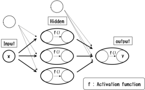
Figure 1: The schematic figure of the feedforward neural network used in this study for the case with the single input and output. The dotted circles mean the bias and the thick arrows indicate the weight. In the final step, we calculate Eq. (16) to obtain the modified integral-path.

In the back-propagation, we choose $\tanh$ for the activation function. In the following, we represents parameters in the neural network as $c=\{c_{i}\}$. Details are shown in Refs. Mori et al. (2017b, 2018). It should be noted that the path optimization method leads the same results with the original theory because of the Cauchy(-Poincare)’s theorem as long as the integral path does not go across singular points, $Je^{-\Gamma}=0$. In the complex Langevin method, singular points induce the problem because it leads the singular drift term in the Langevin-time evolution, the path optimization method can care for it.

In this study, we complexify $A_{3}$ and $A_{8}$ and then $\sigma$ and ${\vec{\pi}}$ are still treated as real variables. Since it is known that the model sign problem can be resolved by the complexification of the temporal gluon fields in the Lefschetz-thimble method Tanizaki et al. (2015), our treatment should work. In addition, such treatment is consistent with the calculation which imposes the ${\cal C}{\cal K}$ symmetry on the fermion determinant at finite density Nishimura et al. (2014, 2015) where ${\cal C}$ and ${\cal K}$ denote the charge conjugation and the complex conjugation, respectively. Unfortunately, the Lefschetz-thimble method is difficult to apply to the PNJL model because we should solve flow equations and it sometimes encounter singular pints of the effective potential. The NJL model with the repulsive vector-type interaction is a typical example Mori et al. (2017a). In comparison, the path optimization method can avoid the problem and thus it is suitable for the PNJL model analysis.

It should be noted that the present path optimization with the machine learning is unsupervised learning because we do not need teacher data to obtain optimized parameters in the neural network. We try to increase the average phase factor compared with that in the previous optimization step. The one attempt to introduce the supervised learning to the study of the sign problem has been done in Ref Alexandru et al. (2017) based on the generalized Lefschetz-thimble method Alexandru et al. (2016).

III.2 Optimization process

We use the following cost function in the calculation;

$${\cal F}[z(t)] =\frac{1}{2}\int d^{n}t~{}|e^{i\theta(t)}-e^{i\theta_{0}}|^{2}\times|J(t)e^{-\Gamma(z(t))}|$$

$$=\int d^{n}t~{}|J(t)e^{-\Gamma(z(t))}|$$

$$\hskip 42.67912pt-\left|\int d^{n}t~{}J(t)e^{-\Gamma(z(t))}\right|,$$ (17)

where

$$\theta(t) =\arg(J(t)e^{-\Gamma(z(t))}),~{}~{}~{}\theta_{0}=\arg({\cal Z}),$$

$$J(t) =\det\Bigl{(}\frac{\partial z_{i}}{\partial t_{j}}\Bigr{)},$$ (18)

with the partition function ${\cal Z}$. In the equation, $z_{i}$ represent complexfied $A_{3}$ and $A_{8}$ and also the real $\sigma$ and ${\vec{\pi}}$. Thus, we have eight dynamical variables. If we wish to take care of the periodicity of the effective potential for $\mathrm{Re}~{}A_{3}$ and $\mathrm{Re}~{}A_{8}$, we should use periodic functional form for those as inputs of the neural network like as Ref. Alexandru et al. (2017). In this study, configurations are well localized in the range $-\pi\leq\mathrm{Re}~{}A_{3}/T\leq\pi$ and $-\pi\leq\mathrm{Re}~{}A_{8}/(T\sqrt{3})\leq\pi$ by using the simple complexification of $A_{3}$ and $A_{8}$. Thus, we do not introduce the periodic form of inputs in this study. This cost function is proportional to $\langle e^{i\theta}\rangle$ and thus it reflects the seriousness of the sign problem Mori et al. (2018). In the physical system, $\theta_{0}$ should be $0$. If we consider $\theta_{0}\neq 0$, we can apply the path optimization method to other systems such as the complex chemical potential.

In the hybrid Monte-Carlo method, we should evaluate the expectation value of the cost function. To do this, we replace the cost function as

$${\cal F}[z(t)]\to\frac{{\cal F}[z(t)]}{\int d^{n}t~{}{\cal P}(t)},$$ (19)

where ${\cal P}$ is the appropriate probability distribution.

In the back-propagation procedure, we need the derivative of the cost function by $c_{i}$. We represent it as $d{\cal F}_{i}$ below. After straightforward calculations, we finally reach the expression;

$$d{\cal F}_{i}(t,c) =|J(t)e^{-\Gamma(z(t))}|$$

$$\times{\rm Re}\left[(1-e^{i(\theta(t)-\theta_{0})})\frac{\partial}{\partial c_{i}}\log(J(t)e^{-\Gamma(z(t))})\right],$$ (20)

In the hybrid Monte-Carlo method, we rewrite Eq. (20) as similar to Eq. (19) with ${\cal P}$. This cost function is responsible to the alignment of the Boltzmann weight with each other on the modified integral path if the points are relevant to the path-integral.

To make our optimization easier, we employ the mini-batch training. The configurations are divided as $N_{\mathrm{config}}=nN_{\mathrm{batch}}$ where $N_{\mathrm{batch}}$ is the batch size and then the learning is performed batch by batch. To include all updation of each batch, the parameters in the feedforward neural network is updated by replacing $dF_{i}$ by its mean-value as

$$d{\cal F}_{i}(t,c)\to\frac{1}{N_{\mathrm{batch}}}\sum_{k=1}^{N_{\mathrm{batch}}}d{\cal F}^{(k)}(t,c).$$ (21)

In one optimization step, we update $n$-times with $N_{\mathrm{batch}}$ configurations.

In this study, we use the simple feedforward neural network with the hidden mono-layer. Input is the original integral path and output is its imaginary part. For the optimizer, we employ Adam algorithm Kingma and Ba (2014);

$$v_{i}^{(j+1)} =\beta_{1}v^{(j)}+(1-\beta_{1})d{\cal F}_{i},$$

$$r_{i}^{(j+1)} =\beta_{2}r^{(j)}+(1-\beta_{2})d{\cal F}_{i}^{2},$$

$${\hat{v}}_{i}^{(j+1)} =\frac{v^{(j+1)}_{i}}{1-\beta_{1}^{j}},~{}~{}~{}{\hat{r}}_{i}^{(j+1)}=\frac{r^{(j+1)}_{i}}{1-\beta_{2}^{j}},$$

$$c^{(j+1)}_{i} =c^{(j)}_{i}-\frac{\eta}{\sqrt{{\hat{r}}^{(j+1)}_{i}}+\epsilon}{\hat{v}^{(j+1)}_{i}},$$ (22)

where $j$ is the fictitious time step, $d{\cal F}_{i}$ means $\partial{\cal F}/{\partial c_{i}}$ and $\beta_{1}$ and $\beta_{2}$ are the smoothing factors of the exponential moving average. This algorithm is based on the AdaGrad algorithm Duchi et al. (2011) and the momentum method with preventing the learning weight decay.

III.3 Simulation setup

The number of units in the hidden layer is set to $N_{\mathrm{unit}}=4$. For Adam algorithm, we use $\eta=0.001$, $\alpha=0.999$, $\beta=0.9$ and $\epsilon=10^{-8}$. In the mini-batch training, we set to $N_{\mathrm{batch}}=10$. These parameters are so called hyper parameters in the machine learning. Initial values of parameters in the neural network are prepared based on Xavier initialization Glorot and Bengio (2010).

In the calculation of the expectation values of operators, we have generated $80000$ configurations analyzed each $50$ trajectories for each optimization step. Then, the expectation values are estimated after $2$ times optimization. Statistic errors are obtained by using the Jack-knife method where the bin number is set to $10$. The expectation value of an operator (${\cal O}$) is obtained via the phase reweighting as

$$\langle{\cal O}\rangle =\frac{\displaystyle\int d^{n}t~{}{\cal O}e^{i\theta}|J(t)e^{-\Gamma(z(t))}|}{\displaystyle\int d^{n}t~{}e^{i\theta}|J(t)e^{-\Gamma(z(t))}|}.$$ (23)

In this study, we calculate the chiral condensate and the Polyakov loop.

IV Numerical results

The $T$-dependence of the chiral condensate and the Polyakov loop at $\mu=0$ is shown in Fig. 2. The mean-field results in the infinite volume limit is also shown as the eye guide.

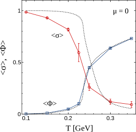
Figure 2: The $T$-dependence of $\langle\sigma\rangle$ and $\langle\Phi\rangle$ at $\mu=0$ where $\langle\sigma\rangle$ is normalized by that at $T=\mu=0$ in the infinite volume limit. The dotted lines are mean-field results in the infinite volume limit as the eye guide.

Because of the finite size effect, $\langle\sigma\rangle$ is deviated from the mean-field results in the infinite volume limit and this result is consistent with results obtained in Ref Cristoforetti et al. (2010). In the present calculation, $V$ depends on $T$ and thus the finite size effect becomes serious when $T$ increases. The expectation values of ${\vec{\pi}}$ are consistent with zero in $2\sigma$ error.

To discuss the model sign problem, we consider the finite $\mu$ below. Figure 3 shows the imaginary part of the effective action.

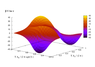
Figure 3: The imaginary part of the effective potential in the $A_{3}$-$A_{8}$ plane with $\sigma^{2}={\vec{\pi}}^{2}=0$. The effective action is normalized as $\beta V{\cal V}$ with $k=64$.

We can clearly see that the effective potential can become complex if we pick up a certain point as the solution of the mean-field approximation.

The $\mu$-dependence of the average phase factor on the original integral-path at $T=100$ and $\mu=300$ is shown in Fig. 4.

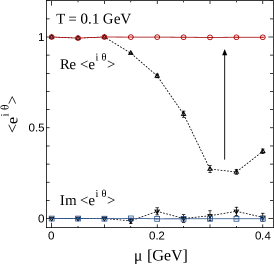
Figure 4: The $\mu$-dependence of $\langle e^{i\theta}\rangle$ at $T=100$ and $\mu=300$ MeV with $k=64$. The dotted and solid lines indicate results on the original and modified integral-paths, respectively. The modified integral-path is obtained after twice optimization.

We also show the results after twice optimization in the figure. It can be clearly seen that $\langle e^{i\theta}\rangle$ becomes small around the chiral transition region, $T\sim 335$ MeV, and then the model sign problem seriously appears. In the present computation, we use $k=64$ and thus $\langle e^{i\theta}\rangle$ does not become small so much, but it will be worse when we consider larger $k$ because $\langle e^{i\theta}\rangle$ is exponentially suppressed by $k$.

To improve the average phase factor, we use the path optimization method. Figure 5 shows the average phase factor at each optimization step with $T=100$ and $\mu=300$ MeV as an example.

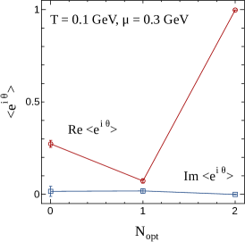
Figure 5: The average phase factor at each optimization step with $T=100$ and $\mu=300$ MeV.

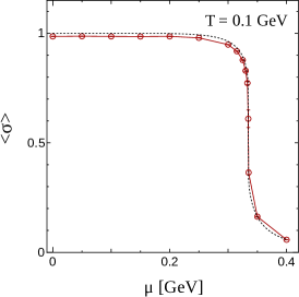
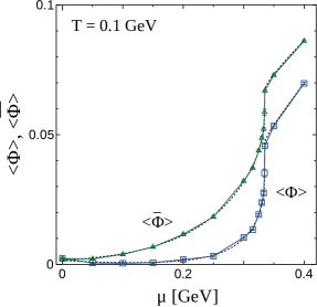
Figure 6: The left (right) panel shows the $\mu$-dependence of $\langle\sigma\rangle$ ($\langle\Phi\rangle$) with $T=100$ and $\mu=300$ MeV where $\langle\sigma\rangle$ is normalized by that at $T=\mu=0$ in the infinite volume limit. The dotted lines are mean-field results with imposing the ${\cal CK}$ symmetry on the fermion determinant in the infinite volume limit as the eye guide.

After one optimization step ($\mathrm{N_{opt}}=1$), the average phase factor becomes worse. Since the starting configurations used in the first optimization are generated on the original integral-path and thus those are expected to be located far from the relevant points of the optimized integral-path and then the average phase factor becomes worse temporally. However, the average phase factor is significantly improved after few optimization steps. In the case at $T=100$ and $\mu=300$ MeV with $k=64$, $\mathrm{N_{opt}}=2$ are enough to make the average phase factor close to $1$. It should be noted that the present tendency of the improvement depends on several initial conditions of parameters and thus we should try with several set of parameters when the optimization is not well worked. Also, an increase of units in the hidden layer may lead to better convergence Frankle and Carbin (2018).

The $\mu$-dependence of the chiral condensate and the Polyakov-loop after performing the path optimization are shown in Fig. 6. The mean-field results in the infinite volume with imposing the ${\cal CK}$ symmetry to the fermion determinant is also shown as the eye guide. We can correctly reproduce the relation $\langle{\bar{\Phi}}\rangle\neq\langle\Phi\rangle$ with $\langle{\bar{\Phi}}\rangle,$$\langle\Phi\rangle\in\mathbb{R}$ in the PNJL model at finite $\mu$ by using the path optimization method. These results mean that the path optimization method can well work in the QCD effective model which has the model sign problem. Also, we can expect that the complexification of the temporal gluon field may be sufficient to control the sign problem in the lattice QCD with the path optimization method since the lattice QCD and the PNJL model share similar properties about the sign problem.

V Summary

In this article, we apply the path optimization method to the Polyakov-loop extended Nambu–Jona-Lasinio (PNJL) model to circumvent the model sign problem. This study is the first attempt to apply the path optimization method to the effective model with dynamical quarks based on QCD. The PNJL model can describe the chiral phase transition and also approximated confinement-deconfinement transition and thus it is a good starting point to investigate the QCD phase structure at finite real chemical potential ($\mu$). Therefore, we choose it as the typical QCD effective model in this article.

The temporal components of the gluon field, $A_{3}$ and $A_{8}$, are complexified and the modified integral path in the complex space is expressed by using the feedforward neural network by minimizing the cost function which reflects the seriousness of the sign problem. Then, the sign problem becomes the optimization problem. Parameters in the feedforward neural network are optimized via the back-propagation method. The neural network tries to increase the average phase factor compared with the previous optimization step and thus it is nothing but the unsupervised learning. The scalar and pseudo-scalar auxiliary fields are treated as real valuables. This treatment is motivated by the Lefschetz-thimble analysis done in Ref. Tanizaki et al. (2015). In the actual optimization process, we use the mini-batch training with Adam algorithm.

We have shown that our treatment of variables of integration works well; the average phase factor is sufficiently improved after the optimization at finite $\mu$. This means that the path optimization method can resolve the model sign problem based on the hybrid Monte-Carlo method. In this study, we use the homogeneous ansatz for the auxiliary fields and thus we cannot go beyond the mean-field approximation, but it is a first step to correctly treat the sign problem in the QCD effective models. By considering the straightforward extension of the present formulation, we will go beyond the mean-field approximation of the QCD effective models. We leave the actual simulation as our future work. From these results, we may expect that the complexification of the temporal gluon fields is the sufficient way to control the sign problem in the lattice QCD with the path optimization method because QCD and the PNJL model share similar properties about the sign problem.